Multi-wavelength emission from magnetically arrested disks around isolated black holes

Abstract

We discuss the prospects for identifying nearest isolated black holes (IBHs) in our Galaxy. IBHs accreting gas from the interstellar medium (ISM) likely form magnetically arrested disks (MADs). We show that thermal electrons in the MADs emit optical signals through the thermal synchrotron process while non-thermal electrons accelerated via magnetic reconnections emit a flat-spectrum synchrotron radiation in the X-ray to MeV gamma-ray ranges. The Gaia catalog will include at most a thousand of IBHs within $\lesssim 1$ kpc that are distributed on and around the cooling sequence of white dwarfs (WDs) in the Hertzsprung-Russell diagram. These IBH candidates should also be detected by eROSITA, with which they can be distinguished from isolated WDs and neutron stars. Followup observations with hard X-ray and MeV gamma-ray satellites will be useful to unambiguously identify IBHs.

1 Introduction

The existence of stellar-mass black holes (BHs) is confirmed by dynamical motion in X-ray binaries (Tetarenko et al., 2016; Corral-Santana et al., 2016) and gravitational-wave detection (Abbott et al., 2021). Stellar-mass BHs are believed to form as an end product of stars of initial masses higher than $\sim$ 25 $M_{\odot}$ (Woosley et al., 2002). Considering the star-formation rate and age of the Universe, there should be roughly $10^{8}$ BHs in our Galaxy (e.g., Abrams & Takada, 2020), suggesting that the nearest BH should be located $\lesssim 50$ pc from the Earth. However, only a few tens of BHs have been discovered, most of which are in X-ray binaries and located $\gtrsim 1$ kpc away from the Earth (Corral-Santana et al., 2016; Tetarenko et al., 2016). Vast majority of stellar-mass BHs in our Galaxy wandering in the interstellar medium (ISM) have yet to be identified.

Wandering BHs, or isolated BHs (IBHs), accrete gas of the ISM via Bondi-Hoyle-Littleton accretion (Edgar, 2004), and accretion flows should be formed around the IBHs. The accretion flows emit multi-wavelength signals, and detection prospects of these signals have been discussed for a long time with various methods and assumptions (Meszaros, 1975; McDowell, 1985; Fujita et al., 1998; Agol & Kamionkowski, 2002; Chisholm et al., 2003; Barkov et al., 2012; Ioka et al., 2017; Tsuna et al., 2018; Tsuna & Kawanaka, 2019).

In this Letter, we discuss prospects to identify nearest IBHs, newly considering two effects. One is the multi-wavelength emission model of magnetically arrested disks (MADs; Narayan et al. 2003; McKinney et al. 2012). MADs are expected to be formed when the mass accretion rate onto the BH is significantly lower than the Eddington rate (Cao, 2011; Kimura et al., 2021), and typical IBHs accrete ISM gas with a highly sub-Eddington rate (Ioka et al., 2017). Thermal electrons are heated up to a relativistic temperature by dissipation of magnetic energy (Chael et al., 2018; Mizuno et al., 2021), and they emit optical signals through thermal synchrotron radiation. MADs also accelerate non-thermal electrons via magnetic reconnections (Hoshino & Lyubarsky, 2012; Guo et al., 2020), which produce X-rays and MeV gamma-rays through synchrotron radiation (Ball et al., 2016; Petersen & Gammie, 2020; Scepi et al., 2021; Ripperda et al., 2021).

The other is to consider the prospects for detection by Gaia (Gaia Collaboration et al., 2016) and eROSITA (Predehl et al., 2021). These satellites will provide complete catalogs of Galactic objects more than ever before, and they likely contain accreting IBHs. In order to distinguish IBHs from other objects, we need to understand multi-wavelength spectra of accreting IBHs and develop a strategy for identifying them. We will describe the multi-wavelength emission model of MADs around IBHs (IBH-MADs), and show how IBH-MADs can be distinguishable from other astronomical objects. We use convention of $Q_{X}=Q/10^{X}$ in cgs unit except the BH mass for which we use $M_{X}=M/10^{X}M_{\odot}$.

2 IBH-MAD model

Table 1: Physical quantities in 5 ISM phases. $n_{\rm ISM}$, $C_{s,\rm ISM}$, $H_{\rm ISM}$, $\xi_{0}$ are the number density, effective sound velocity, scale height, and volume filling factor of the ISM phases. We mainly discuss Cold HI, Warm HI, and Warm HII.

ISM phase	$n_{\rm ISM}$	$C_{s,\rm ISM}$	$H_{\rm ISM}$	$\xi_{0}$
	[cm-3]	[km s-1]	[kpc]
Molecular clouds	$10^{2}$	10	0.075	0.001
Cold HI	$10$	10	0.15	0.04
Warm HI	0.3	10	0.50	0.35
Warm HII	0.15	10	1.0	0.2
Hot HII	0.002	150	3.0	0.43

Accretion rates onto IBHs strongly depend on the physical properties of the ISM and IBH. We consider five-phase ISM given by Bland-Hawthorn & Reynolds (2000), which is also used in the literature (e.g., Agol & Kamionkowski, 2002; Ioka et al., 2017; Tsuna et al., 2018). The physical parameters characterizing each ISM phase is tabulated in Table 1. We find that Gaia can detect IBHs in hot HII medium only when they are extremely close ($d\lesssim 10$ pc) and/or massive ($M\gtrsim 40~{}M_{\odot}$). Also, Gaia may be unable to measure the intrinsic color of IBHs in molecular clouds due to strong dust extinction, and thus it is difficult to identify IBHs in molecular clouds (but see e.g., Matsumoto et al. 2018). Hence, we hereafter focus on the other three phases.

We estimate the physical properties of IBH-MADs. Since the accretion rate is much lower than the Eddington rate, $\dot{M}_{\rm Edd}=L_{\rm Edd}/c^{2}\simeq 1.4\times 10^{18}M_{1}\rm~{}g~{}s^{-1}$, the radiatively inefficient accretion flow (RIAF; Ichimaru 1977; Narayan & Yi 1994; Yuan & Narayan 2014) is formed. According to recent general relativistic magnetohydrodynamic (GRMHD) simulations, RIAFs can produce outflows and create large-scale poloidal magnetic fields even starting from purely toroidal magnetic field (Liska et al., 2020). These poloidal fields are efficiently carried to the IBH, which likely results in formation of a MAD around the IBH (Cao, 2011; Ioka et al., 2017; Kimura et al., 2021). Introducing a reduction parameter of the mass accretion rate, $\lambda_{w}\leq 1$, due to outflows and convection (Blandford & Begelman, 1999; Quataert & Gruzinov, 2000; Yuan et al., 2015; Inayoshi et al., 2018), the accretion rate onto an IBH can be estimated as

$$\dot{M}_{\bullet} \approx \lambda_{w}\frac{4\pi G^{2}M^{2}\mu_{\rm ISM}m_{p}n_{\rm ISM}}{\left(C_{s}^{2}+v_{k}^{2}\right)^{3/2}}$$

$$\simeq 7.3\times 10^{10}\lambda_{w,0}M_{1}^{2}n_{\rm ISM,-1}\left(\frac{\sqrt{C_{s}^{2}+v_{k}^{2}}}{40\rm~{}km~{}s^{-1}}\right)^{-3}\rm~{}g~{}s^{-1},$$

where $G$ is the gravitational constant, $M$ and $v_{k}$ are the mass and the proper-motion velocity of the IBH, respectively, $m_{p}$ is the proton mass, and $\mu_{\rm ISM}\simeq 1.26$, $n_{\rm ISM}$, and $C_{s}$ are the mean atomic weight, number density, and sound speed of the ISM gas (see Table 1), respectively. We use $\lambda_{w}=1$ as a reference value for simplicity, but we will discuss the cases with a low value of $\lambda_{w}$ in Section 5. We assume $v_{k}\simeq 40\rm~{}km~{}s^{-1}$ as a reference value as in Ioka et al. (2017)

The radial velocity, proton temperature, gas number density, and magnetic field of MADs can be estimated to be (Kimura et al., 2019b, 2021, 2021)

$$V_{R} \approx \frac{1}{2}\alpha V_{K}\simeq 1.5\times 10^{9}\mathcal{R}_{1}^{-1/2}\alpha_{-0.5}\rm~{}cm~{}s^{-1},$$ (2)

$$k_{B}T_{p} \approx \frac{GMm_{p}}{4R}\simeq 23\mathcal{R}_{1}^{-1}\rm~{}MeV$$ (3)

$$N_{p} \approx \frac{\dot{M}_{\bullet}}{4\pi RHV_{R}\mu_{\rm ISM}m_{p}}$$

$$\simeq 2.3\times 10^{10}\dot{M}_{\bullet,11}M_{1}^{-2}\mathcal{R}_{1}^{-3/2}\alpha_{-0.5}^{-1}\rm~{}cm^{-3},$$

$$B = \sqrt{\frac{8\pi N_{p}k_{B}T_{p}}{\beta}}$$

$$\simeq 1.5\times 10^{4}\dot{M}_{\bullet,11}^{1/2}M_{1}^{-1}\mathcal{R}_{1}^{-5/4}\alpha_{-0.5}^{-1/2}\beta_{-1}^{-1/2}\rm~{}G,$$

where $\mathcal{R}=R/R_{G}$ is the size of the emission region normalized by the gravitational radius, $R_{G}=GM/c^{2}$, $\alpha$ is the viscous parameter (Shakura & Sunyaev, 1973), $H\approx R/2$ is the scale height, and $\beta$ is the plasma beta.

Inside MADs, electrons are heated up to a relativistic temperature by magnetic energy dissipation, such as magnetic reconnections (Rowan et al., 2017; Hoshino, 2018) and the turbulence cascades (Howes, 2010; Kawazura et al., 2019). We parameterize the total heating rate and electron heating rate as

$$Q_{\rm thrml} = \epsilon_{\rm dis}(1-\epsilon_{\rm NT})\dot{M}_{\bullet}c^{2},$$ (6)

$$Q_{e,\rm thrml} = f_{e}Q_{\rm thrml}$$

$$\simeq 2.7\times 10^{30}\left(\frac{f_{e}\epsilon_{\rm dis}(1-\epsilon_{\rm NT})}{0.3\cdot 0.15\cdot 0.67}\right)\dot{M}_{\bullet,11}\rm~{}erg~{}s^{-1},$$

where $\epsilon_{\rm dis}$ is the ratio of dissipation to accretion energies, $\epsilon_{\rm NT}$ is the ratio of non-thermal particle production to dissipation energy, and $f_{e}$ the electron heating fraction. Considering the trans-relativistic magnetic reconnection, we use the electron heating prescription given by Rowan et al. (2017); Chael et al. (2018):

$$f_{e}\approx\frac{1}{2}\exp\left(-\frac{1-4\beta\sigma_{B}}{0.8+\sqrt{\sigma_{B}}}\right),$$ (8)

where $\sigma_{B}=B^{2}/(4\pi N_{p}m_{p}c^{2})\simeq 0.5\mathcal{R}_{1}^{-1}\beta_{-1}^{-1}$ is the magnetization parameter. We assume that the proton temperature is sub-relativistic, which is reasonable for the bulk of the accretion flows. We obtain $f_{e}\sim 0.3$ with our reference parameter set.

3 Photon spectra from IBH-MADs

We calculate the photon spectrum from IBH-MADs using the method in Kimura et al. (2021) (see also Kimura et al. 2015, 2019a; Kimura & Toma 2020), where we include both thermal and non-thermal components of electrons and treat them as separate components. Thermal electrons emit broadband photons by thermal synchrotron, bremsstrahlung, and Comptonization processes. Non-thermal electrons emit broadband photons by synchrotron emission, and we can ignore other emission processes in the MADs. We also calculate emissions induced by non-thermal protons, but we find that their contribution is negligible.

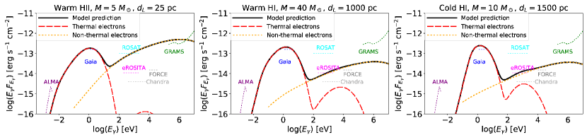
Figure 1: Broadband spectra from IBH-MADs. The thick-solid, thick-dashed, and thick-dotted lines are total, photon spectra by thermal electrons, and photon spectra by non-thermal electrons. The thin-dashed lines are sensitivity curves for ALMA (purple: 30 min; ALMA Sensitivity Calculator), Gaia (blue; 20 mag; Gaia Collaboration et al. 2018), eROSITA (magenta; 4-year survey; Predehl et al. 2021), Chandra (gray; 10 ks; CXO website), FORCE (darkgray; 100 ks; Nakazawa et al. 2018), and GRAMS (green; 3 year; Aramaki et al. 2020). ISM phase, black hole mass, and distances are shown in each panel. Other parameters are $\mathcal{R}=10$, $\alpha=0.3$, $\beta=0.1$, $\epsilon_{\rm dis}=0.15$, $\epsilon_{\rm NT}=0.33$, $\eta_{\rm acc}=5$, and $s_{\rm inj}=1.3$.

The thermal electrons emit optical photons by thermal synchrotron radiation. For cases with low $\dot{M}_{\bullet}$, the cooling processes are so inefficient that the radiative cooling cannot balance the heating before falling to the IBH. Then, the electron temperature is determined by $k_{B}T_{e,\rm adi}\approx f_{e}k_{B}T_{p}\simeq 7.0(f_{e}/0.3)\mathcal{R}_{1}^{-1}$ MeV. For high $\dot{M}_{\bullet}$, the electron temperature is determined by the balance between the heating and cooling, i.e., $Q_{e,\rm thrml}=L_{\rm thrm}(T_{e,\rm rad})$, where $L_{\rm thrm}(T_{e,\rm rad})$ is the radiative cooling rate. The electron temperature in IBH-MADs are given by $T_{e}={\rm min}(T_{e,\rm adi},~{}T_{e,\rm rad})$.

Because of their lower accretion rate compared to quiescent X-ray binaries by 2-3 orders of magnitude, IBH-MADs are optically thin for synchrotron-self absorption (SSA) at the synchrotron peak frequency in the most parameter space. This feature is different from any other RIAF systems, such as quiescent X-ray binaries (Narayan et al., 1996; Kimura et al., 2021), radio galaxies (Kimura & Toma, 2020), low-luminosity AGNs (Nemmen et al., 2014; Kimura et al., 2015, 2019a, 2021), and Sgr A* (Narayan et al., 1995; Manmoto et al., 1997; Yuan et al., 2003). Since the optically thin thermal synchrotron emission has a gradual spectral cutoff (Mahadevan et al., 1996), the peak frequency of the synchrotron spectrum is $\simeq 25$ times higher than the canonical synchrotron frequency, $\nu_{\rm syn}=3eB\theta_{e}^{2}/(4\pi m_{e}c)$, where $\theta_{e}=k_{B}T_{e}/(m_{e}c^{2})$. Then, the peak frequency of the thermal synchrotron emission is estimated to be

$$\nu_{\rm syn,pk}\approx\frac{75eB\theta_{e}^{2}}{4\pi m_{e}c}\simeq 2.0\times 10^{14}B_{4}\mathcal{R}_{1}^{-2}\left(\frac{f_{e}}{0.3}\right)^{2}\rm~{}Hz,$$ (9)

where we use $T_{e}=T_{e,\rm adi}$. The luminosity of the thermal synchrotron emission is roughly estimated to be

$$\nu_{\rm syn,pk}L_{\nu_{\rm syn,pk}}\approx\frac{4}{3}(3\theta_{e})^{2}\frac{\sigma_{T}cB^{2}}{8\pi}(\pi R^{3}N_{p})$$

$$\simeq 9.3\times 10^{28}\dot{M}_{\bullet,11}^{2}M_{1}^{-1}\mathcal{R}_{1}^{-3}\alpha_{-0.5}^{-2}\beta_{-1}^{-1}\left(\frac{f_{e}}{0.3}\right)^{2}\rm~{}erg~{}s^{-1}.$$

Comparing Equations (2) and (3), the critical mass accretion rate above which the cooling is efficient can be estimated to be

$$\dot{M}_{\rm cl}\simeq 2.9\times 10^{12}M_{1}\mathcal{R}_{1}^{3}\alpha_{-0.5}^{2}\beta_{-1}\left(\frac{f_{e}}{0.3}\right)^{-1}$$ (11)

$$\times\left(\frac{\epsilon_{\rm dis}(1-\epsilon_{\rm NT})}{0.15\cdot 0.67}\right)\rm~{}g~{}s^{-1}.$$

With our reference parameters, typical IBH-MADs in the warm media are in the adiabatic regime, while those in the cold medium are in the cooling regime.

Magnetic reconnections accelerate non-thermal electrons which emit X-rays and soft gamma-rays by synchrotron radiation. We consider non-thermal particle injection, cooling, and escape processes, and solve the steady-state transport equation to obtain the number spectrum, $N_{E_{e}}$ (see Kimura & Toma 2020; Kimura et al. 2021 for details). The injection spectrum is assumed to be a power law with an exponential cutoff, i.e., $\dot{N}_{E_{e},\rm ing}\propto E_{e}^{-s_{\rm inj}}\exp(-E_{e}/E_{e,\rm cut})$, where $E_{e,\rm cut}$ is the cutoff energy and $s_{\rm inj}$ is the injection spectral index. Although earlier 2D particle-in-cell (PIC) simulations result in a cutoff energy of $E_{\rm cut}\sim 4\sigma_{B}$ (Werner et al., 2016), long-term calculations revealed that the cutoff energy is increasing with time (Petropoulou & Sironi, 2018; Zhang et al., 2021). Since the dynamical timescale of the accretion flow is much longer than the timescales of kinetic plasma phenomena, we determine $E_{\rm cut}$ by the balance between the acceleration and cooling processes. The injection rate is normalized by $\int\dot{N}_{E_{e},\rm inj}E_{e}dE_{e}=f_{e}\epsilon_{\rm NT}\epsilon_{\rm dis}\dot{M}_{\bullet}c^{2}$. We consider only the synchrotron cooling as the other processes are negligible. We consider both advective (infall to the IBH) and diffusive escapes. The acceleration time is phenomenologically set to be $t_{\rm acc}=\eta_{\rm acc}E_{e}c/(eBV_{A}^{2})$, where $V_{A}=B/\sqrt{4\pi m_{p}N_{p}}$ is the Alfven velocity and $\eta_{\rm acc}$ is the acceleration efficiency parameter.

In the range of our interest, the synchrotron cooling limits the maximum energy, and the synchrotron cutoff energy is estimated to be

$$E_{\gamma,\rm cut}\approx\frac{3e^{2}h_{p}\beta_{A}^{2}}{m_{e}c\sigma_{T}\eta_{\rm acc}}\simeq 15\left(\frac{\beta_{A}}{0.7}\right)^{2}\left(\frac{\eta_{\rm acc}}{5}\right)^{-1}\rm~{}MeV.$$ (12)

The peak luminosity for the non-thermal synchrotron process is roughly estimated to be $E_{\gamma}L_{E_{\gamma}}\approx f_{e}\epsilon_{\rm NT}\epsilon_{\rm dis}\dot{M}c^{2}$. The cooling break energy is given by equating infall time to the cooling time: $E_{\gamma,\rm cl}\approx h_{p}eB\gamma_{e,\rm cl}^{2}/(2\pi m_{e}c)\approx 1.2\times 10^{2}B_{4}\gamma_{e,\rm cl,3}^{2}$ eV, where $\gamma_{e,\rm cl}\approx{\rm max}(1,6\pi m_{e}cV_{R}/(\sigma_{T}B^{2}R))\simeq 7.7\times 10^{2}V_{R,9}B_{4}^{-2}R_{7}^{-1}$ is the cooling break Lorentz factor. The X-ray band is typically above the cooling break energy, and thus the photon index in the X-ray band is $\Gamma_{X}=(s_{\rm inj}+2)/2\simeq 1.65$ with $s_{\rm inj}=1.3$ (see Section 5 for discussion on the value of $s_{\rm inj}$). Then, the X-ray luminosity is estimated to be

$$E_{X}L_{X}\simeq 1.3\times 10^{29}\dot{M}_{\bullet,11}f_{X,-1}\left(\frac{f_{e}\epsilon_{\rm NT}\epsilon_{\rm dis}}{0.3\cdot 0.33\cdot 0.15}\right)\rm~{}erg~{}s^{-1},$$ (13)

where $f_{X}=(E_{X}/E_{\gamma,\rm cut})^{2-\Gamma_{X}}\sim 0.1$ is the correction factor. IBH-MADs in the adiabatic regime roughly exhibit $L_{X}/L_{\rm opt}\sim 1$ with our reference parameters, as seen by Equations (3) and (13). In the cooling regime of $\dot{M}_{\bullet}>\dot{M}_{\rm cl}$, both thermal and non-thermal electrons emit all the energies via synchrotron emission. Then, we can write $L_{X}/L_{\rm opt}\approx f_{X}\epsilon_{\rm NT}/(1-\epsilon_{\rm NT})\sim 0.05$ with our reference parameters.

Figure 1 shows the broadband photon spectra from IBH-MADs, whose parameters are shown in each panel and the caption. The parameters in our MAD model are calibrated using the gamma-ray data of radio galaxies (Kimura & Toma, 2020) and the multi-wavelength data of quiescent X-ray binaries (Kimura et al., 2021). The thermal synchrotron emission produces optical signals that is detectable by Gaia. The synchrotron emission by non-thermal electrons produce power-law photons from X-ray to MeV gamma-ray ranges. The IBHs detectable by Gaia should be detected by eROSITA (Predehl et al., 2021). SSA is effective in radio and sub-mm bands, and thus, it is challenging to detect IBH-MADs by radio telescopes, such as ALMA (see Section 5 for radio signals from jets associated with IBH-MADs). For a low accretion rate, the advection cooling is effective for thermal electrons, while the radiative cooling is efficient for non-thermal electrons. Then, emission by non-thermal electrons can be more luminous than that by thermal electrons, despite we choose $\epsilon_{\rm NT}<1-\epsilon_{\rm NT}$, as seen in the left panel of Figure 1.

4 Strategy to identify IBHs

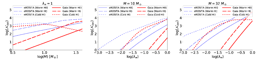
Figure 2: Expected numbers of IBHs detected by Gaia (thick-red) and eROSITA (thin-blue) as a function of $M$ (left) and $\lambda_{w}$ (middle and right) in various ISM phases. The solid, dashed, and dotted lines are for warm HII, warm HI, and cold HI, respectively.

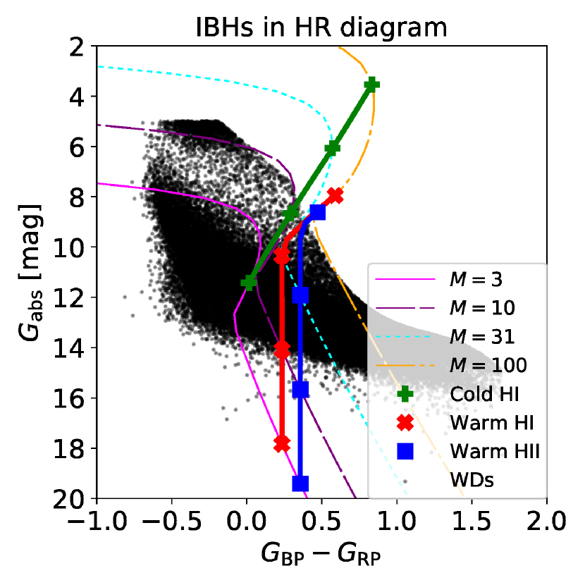
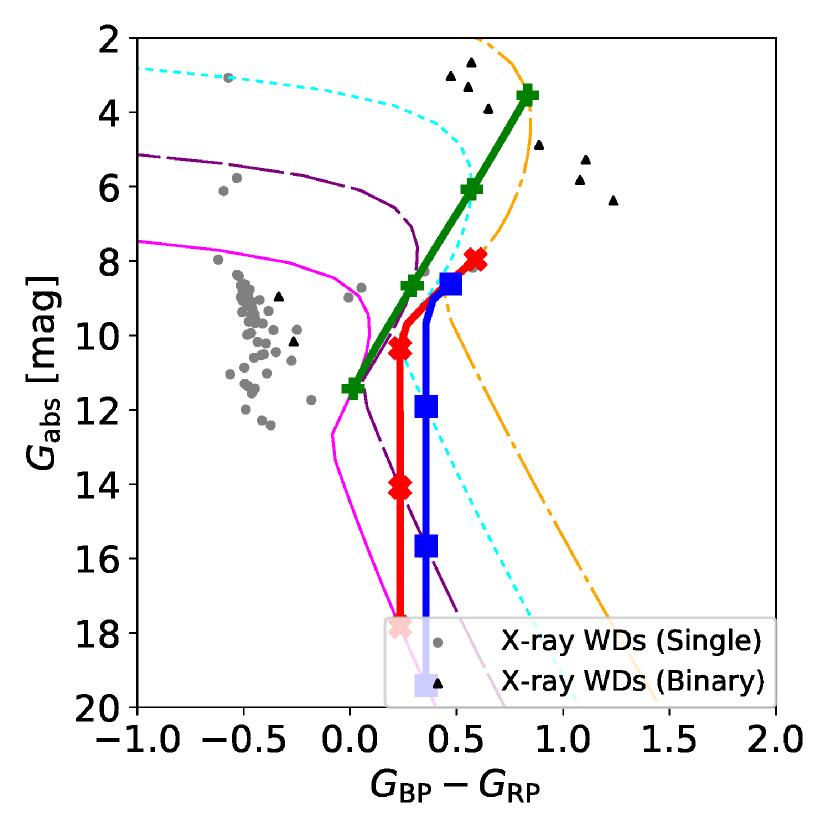
Figure 3: Regions where IBH-MADs occupy in the HR diagram. The thick lines with symbols indicate the IBH-MADs in cold HI (green plus), warm HI (red cross), and warm HII (blue square). The thick lines are obtained by changing the IBH mass. The thin lines depict the sequences of an IBH with various values of the mass accretion rate. In the top panel, we also plot WD candidates detected by Gaia (Gentile Fusillo et al., 2019). In the bottom panel, we plot X-ray emitting WDs (grey circles and black triangles) in Fleming et al. (1996), and their classification is given by Dufour et al. (2017).

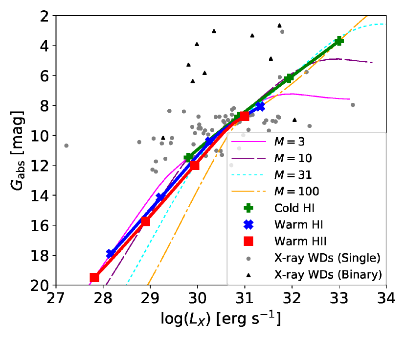
Figure 4: The relation between X-ray luminosity and Gaia G-band absolute magnitude for IBHs (thin and thick lines) and X-ray emitting WDs (grey circles and black triangles).

First, we roughly estimate the number of IBHs that can be detected by Gaia or eROSITA. We estimate the detection horizon, $d_{i,\rm det}={\rm min}(\sqrt{L_{i,\rm band}/(4\pi f_{i,\rm sen})},~{}d_{\rm max})$, where $L_{i,\rm band}$ is the luminosity in the energy band for the detector (330 nm – 1050 nm for Gaia; 0.2 keV – 2.3 keV for eROSITA), $f_{i,\rm sen}$ is the sensitivity of the detector (20 mag for Gaia DR5 and $1.1\times 10^{-14}\rm~{}erg~{}s^{-1}~{}cm^{-2}$ for the eROSITA four-year survey), and $d_{\rm max}$ is the maximum distance. We set $d_{\rm max}=2$ kpc because Gaia cannot precisely measure the parallax for faint sources and the extinction and attenuation may affect the detectability.

The expected number of detectable IBH candidates can be estimated to be

$$\mathcal{N}_{\rm det}(M)\sim M\frac{dN_{\rm IBH}}{dMdV}\xi_{0}{\rm~{}min}\left(\frac{4\pi}{3}d_{i,\rm det}^{3},~{}2\pi H_{\rm ISM}d_{i,\rm det}^{2}\right),$$ (14)

where $H_{\rm ISM}$ is the scale height of each ISM phase (see Table 1) and $dN_{\rm IBH}/(dMdV)$ is the number of IBHs per unit mass and volume. We assume a simple power-law mass spectrum with spectral index suggested by the gravitational-wave data: $dN_{\rm IBH}/dM\propto M^{-\gamma}$ with $\gamma\sim 2.6$ (Abbott et al., 2021). We consider the mass range of IBHs of $3.2~{}M_{\odot}\leq M\leq 50~{}M_{\odot}$. The mass-integrated number density of IBHs is set to be $dN_{\rm IBH}/dV=\int(dN/dMdV)dM=10^{5}\rm~{}kpc^{-3}$, which is roughly consistent with N-body simulations by Tsuna et al. (2018). The resulting values of $\mathcal{N}_{\rm det}$ are plotted in the left panel of Figure 2. We can see that both eROSITA and Gaia will detect $\sim 10^{3}$ IBHs in cold HI medium in a broad mass range. Several hundreds (around a hundred) of low-mass ($M\sim 5~{}M_{\odot}$) IBHs in warm HI (warm HII) medium can be discovered by eROSITA, while Gaia can detect only $\sim 10$ ($\sim 1$) low-mass IBHs in warm HI (warm HII) medium. More than a thousand high mass IBHs in warm HI can be detected by both Gaia and eROSITA. We should note that both the mass spectrum and volumetric density of IBHs are very uncertain. The data by OGLE microlensing surveys suggest a flatter mass spectrum of IBHs with $\gamma\simeq 0.92$ (Mroz et al., 2021). Also, the Sun is located in a local bubble (Frisch et al., 2011), which may decrease the detectable number of IBHs within $\sim 100$ pc.

The sensitivity of the ROSAT All-Sky Survey (RASS) is $\sim 10^{-13}\rm~{}erg~{}s^{-1}~{}cm^{-2}$ (Boller et al., 2016), which is an order of magnitude lower than that of eROSITA. RASS should detect 0.01 times less IBH candidates than eROSITA, which should contain $\sim 10$ low-mass IBH candidates. This number is similar to that of RASS unidentified sources in the northern sky (Krautter et al., 1999), and thus, our model is consistent with the currently available X-ray data.

Next, we discuss strategy to identify IBH candidates. The Hertzsprung-Russell (HR) diagram is useful to classify the objects. Figure 3 exhibits the regions where IBH-MADs occupy in the HR diagram with our reference parameters. We can see that low-mass IBH-MADs in the warm media are located at a fainter and bluer region than the white dwarf (WD) cooling sequence. Ultra-cool WDs and neutron stars (NS), including both pulsars and thermally emitting NSs, can be located in the same region. We can utilize the X-ray feature to distinguish IBH-MADs from them. Pulsars and thermally emitting NSs have high values of X-ray to optical luminosity ratio, $L_{X}/L_{\rm opt}\gg 1$ (Bühler & Blandford, 2014; Kaplan et al., 2011), while low-mass IBHs exhibit $L_{X}/L_{\rm opt}\sim 1$ as discussed in Section 3. In addition, the expected number of detectable isolated NSs are lower than that of IBH-MADs (Toyouchi et al., 2021). Isolated WDs may emit X-rays, but the X-ray emitting WDs detected by RASS (Fleming et al., 1996; Agüeros et al., 2009) are bluer and more luminous in G bands than low-mass IBHs, as shown in the bottom panel of Figure 3 and Figure 4. Ultra-cool WDs are unlikely to emit bright X-rays. Since eROSITA can detect almost all IBHs detected by Gaia, we will be able to identify good low-mass IBH candidates using Gaia and eROSITA data.

High-mass IBHs of $M\gtrsim 50M_{\odot}$ in warm HI/warm HII or medium-mass ($M\sim 10~{}M_{\odot}$) IBHs in cold HI are located in a redder and brighter region of the WD cooling sequence. This region might be contaminated by binaries consisting of a WD and a main-sequence star, as seen in the bottom panel of Figure 3. They can emit X-rays through the magnetic activity, and the values of $L_{X}/L_{\rm opt}$ are also similar to the IBH-MADs (see Figure 4). Nevertheless, we can discriminate them by multi-band photometric observations. WD-star binaries are expected to have a two-temperature blackbody spectrum in optical bands, while IBH-MADs should exhibit a single smooth component of thermal synchrotron spectrum.

IBH-MADs are likely variable within dynamical timescale, and thus, we should expect strong intra-night variability compared to WDs. ULTRACAM can detect sub-second variability, which is a smoking-gun signal to distinguish IBH-MADs from WDs. Also, IBH-MADs should not show any absorption and emission lines. Therefore, spectroscopic and photometric follow-up observations in both X-ray and optical bands may be useful to distinguish IBHs from WDs. Considering the limiting magnitude of Gaia ($\sim$20 mag), IBH candidates are detectable with 2-meter telescopes for photometric follow-up observations, or with 4-meter telescopes for spectroscopic observations. Detailed soft X-ray spectra of IBH-MADs can be obtained by current and near future X-ray satellites, including Chandra (see Figure 1) and XRISM (XRISM Science Team, 2020). Besides, IBH-MADs can be detected by future hard X-ray (FORCE: Nakazawa et al. 2018) and MeV gamma-ray (e.g., GRAMS: Aramaki et al. 2020) detectors as seen in Figure 1, which will strongly support our IBH-MAD scenario. If IBH-MADs are bright enough as in the left panel of Figure 1, NuSTAR is also able to detect them.

5 Discussion

We have discussed strategy to identify IBHs based on multi-wavelength emission model of MADs. Thermal and non-thermal electrons in MADs emit optical and X-ray signal, respectively, which are detectable by Gaia and eROSITA. We can discriminate IBH-MADs from other objects using $L_{X}/L_{\rm opt}$ and the HR diagram. Hard X-ray and MeV gamma-ray detections will enable us to firmly identify IBHs.

The mass accretion rate onto IBH-MADs can be lower than our reference parameter set due to a lower $\lambda_{w}$ (outflows/convection) or a higher $v_{k}$. In order to check the detection prospects with lower values of $\dot{M}_{\bullet}$, we also calculate emission from IBH-MADs with various values of $\dot{M}_{\bullet}$. The thin lines in Figure 3 show the tracks for IBH-MADs of a fixed mass with various $\dot{M}_{\bullet}$. On each line, IBH-MADs with higher values of $\dot{M}_{\bullet}$ reside an upper region, and we can see three branches in each line. For the low-$\dot{M}_{\bullet}$ branch, the electron temperature is independent of $\dot{M}_{\bullet}$ owing to inefficient radiative cooling. The magnetic fields are stronger and the synchrotron frequency is higher for IBH-MADs with a higher $\dot{M}_{\bullet}$, and thus, IBH-MADs are bluer when more luminous. In the medium-$\dot{M}_{\bullet}$ branch, the radiative cooling is efficient enough to balance the heating. In this case, the electron temperature is lower for a higher $\dot{M}_{\bullet}$, making the branch redder when more luminous. For the high $\dot{M}_{\bullet}$ branch, the Gaia band is optically thick for the SSA process. Then, the spectral shape below the absorption frequency is given by the Rayleigh-Jeans spectrum, exhibiting a very bluer color when more luminous. The middle and right panels of Figure 2 indicate the expected detection number as a function of $\lambda_{w}$. Gaia cannot detect 10-$M_{\odot}$ IBHs in warm media for $\lambda_{w}<0.1$, while 10-$M_{\odot}$ IBHs in cold HI can be detectable by Gaia for $\lambda_{w}\gtrsim 0.01$. eROSITA can still detect several tens of 30-$M_{\odot}$ IBH-MADs even for $\lambda_{w}\sim 0.001$. Optical followup observations of eROSITA unidentified sources will be important to identify IBHs for the cases with $\lambda_{w}<0.01$. Observations of nearby low-luminosity AGNs, including Sgr A*, indicate $\lambda_{w}\sim 0.001-0.01$ (e.g., Inayoshi et al., 2018), while the values for IBHs are currently unclear.

The value of electron heating fraction, $f_{e}$, is also uncertain. The electron heating prescription by Hoshino (2018) suggests $f_{e}\sim 0.1$. This leads IBH-MADs to redder regions in the HR diagram ($G_{\rm BP}-G_{\rm RP}\sim 1-2$) . Also, IBH-MADs is luminous in X-rays compared to the optical band as $L_{X}/L_{\rm opt}\propto f_{e}^{-1}$ (see Equations (3) and (13)). Despite these uncertainties, our strategy of IBH identification should still work even with low values of $f_{e}$, because faint and red WDs are very unlikely to emit X-rays. Therefore, we suggest to search for IBH candidates in a broad region of the HR diagram using X-ray data.

The spectral index of reconnection acceleration may be softer than our assumption of $s_{\rm inj}=1.3$, but our conclusions are unaffected as long as we use $s_{\rm inj}\lesssim 2$. Recent 3D particle-in-cell (PIC) simulations support a hard spectral index of $s_{\rm inj}\sim 1$ (Zhang et al., 2021), and long-term 2D PIC simulations suggest $s_{\rm inj}\simeq 2$ (Petropoulou & Sironi, 2018). These results support our assumption. In contrast, other 2D PIC simulations indicate much softer spectra ($s_{\rm inj}\sim 3-4$) at a high-energy range of $E_{e}\gtrsim\sigma_{B}m_{e}c^{2}$ (Ball et al., 2018; Werner et al., 2018; Hakobyan et al., 2021). If particle acceleration by magnetic reconnections results in a soft spectral index, the subsequent stochastic acceleration by turbulence is necessary (Comisso & Sironi, 2018) to emit strong X-ray signals.

The IBHs may emit radio and sub-mm signals. Although IBH-MADs cannot produce detectable radio signals, compact jets are highly likely launched by MADs (Tchekhovskoy et al., 2011). Such jets may produce radio signals as detected from a few quiescent X-ray binaries (e.g., Hynes et al., 2009; Gallo et al., 2019). The radio luminosity correlates with X-ray luminosity in the low-hard state: $L_{R}\sim 1.4\times 10^{29}L_{X,35}^{0.61}\rm~{}erg~{}s^{-1}$ (Gallo et al., 2014). If we extrapolate this relation to the regime of IBHs, the radio flux can be estimated to be $F_{R}\sim 0.63~{}L_{X,28}^{0.61}(d/100\rm~{}pc)^{-2}$ mJy. Thus, the signals from compact jets are detectable by current radio telescopes, such as ALMA and VLA. These signals may be detectable by ongoing radio surveys, such as Very Large Array Sky Survey (VLASS; Lacy et al., 2020), ThunderKAT (Fender et al., 2017), and ASKAP Survey for Variable and Slow Transients (VAST; Murphy et al., 2013). Current observational data of quiescent X-ray binaries are not precise enough to obtain the $L_{R}-L_{X}$ relation. $L_{R}$ might decrease more rapidly than $L_{X}$ in a highly sub-Eddington regime (Rodriguez et al., 2020), which leads to 1–2 orders of magnitude lower radio flux. Even in this case, the next-generation radio facilities will be able to detect radio signals from IBHs, which will provide another support of the IBH-MAD scenario.

References

- Abbott et al. (2021) Abbott, R., et al. 2021, Phys. Rev. X, 11, 021053, doi: 10.1103/PhysRevX.11.021053
- Abbott et al. (2021) Abbott, R., Abbott, T. D., Abraham, S., et al. 2021, ApJ, 913, L7, doi: 10.3847/2041-8213/abe949
- Abrams & Takada (2020) Abrams, N. S., & Takada, M. 2020, ApJ, 905, 121, doi: 10.3847/1538-4357/abc6aa
- Agol & Kamionkowski (2002) Agol, E., & Kamionkowski, M. 2002, MNRAS, 334, 553, doi: 10.1046/j.1365-8711.2002.05523.x
- Agüeros et al. (2009) Agüeros, M. A., Anderson, S. F., Covey, K. R., et al. 2009, ApJS, 181, 444, doi: 10.1088/0067-0049/181/2/444
- Aramaki et al. (2020) Aramaki, T., Adrian, P. O. H., Karagiorgi, G., & Odaka, H. 2020, Astroparticle Physics, 114, 107, doi: 10.1016/j.astropartphys.2019.07.002
- Ball et al. (2016) Ball, D., Özel, F., Psaltis, D., & Chan, C.-k. 2016, ApJ, 826, 77, doi: 10.3847/0004-637X/826/1/77
- Ball et al. (2018) Ball, D., Sironi, L., & Özel, F. 2018, ApJ, 862, 80, doi: 10.3847/1538-4357/aac820
- Barkov et al. (2012) Barkov, M. V., Khangulyan, D. V., & Popov, S. B. 2012, MNRAS, 427, 589, doi: 10.1111/j.1365-2966.2012.22029.x
- Bland-Hawthorn & Reynolds (2000) Bland-Hawthorn, J., & Reynolds, R. 2000, Gas in Galaxies, ed. P. Murdin, 2636, doi: 10.1888/0333750888/2636
- Blandford & Begelman (1999) Blandford, R. D., & Begelman, M. C. 1999, MNRAS, 303, L1, doi: 10.1046/j.1365-8711.1999.02358.x
- Boller et al. (2016) Boller, T., Freyberg, M. J., Trümper, J., et al. 2016, A&A, 588, A103, doi: 10.1051/0004-6361/201525648
- Bühler & Blandford (2014) Bühler, R., & Blandford, R. 2014, Reports on Progress in Physics, 77, 066901, doi: 10.1088/0034-4885/77/6/066901
- Cao (2011) Cao, X. 2011, ApJ, 737, 94, doi: 10.1088/0004-637X/737/2/94
- Chael et al. (2018) Chael, A., Rowan, M., Narayan, R., Johnson, M., & Sironi, L. 2018, MNRAS, 478, 5209, doi: 10.1093/mnras/sty1261
- Chisholm et al. (2003) Chisholm, J. R., Dodelson, S., & Kolb, E. W. 2003, ApJ, 596, 437, doi: 10.1086/377628
- Comisso & Sironi (2018) Comisso, L., & Sironi, L. 2018, Phys. Rev. Lett., 121, 255101, doi: 10.1103/PhysRevLett.121.255101
- Corral-Santana et al. (2016) Corral-Santana, J. M., Casares, J., Muñoz-Darias, T., et al. 2016, A&A, 587, A61, doi: 10.1051/0004-6361/201527130
- Dufour et al. (2017) Dufour, P., Blouin, S., Coutu, S., et al. 2017, in Astronomical Society of the Pacific Conference Series, Vol. 509, 20th European White Dwarf Workshop, ed. P. E. Tremblay, B. Gaensicke, & T. Marsh, 3. https://arxiv.org/abs/1610.00986
- Edgar (2004) Edgar, R. 2004, New Astron. Rev., 48, 843, doi: 10.1016/j.newar.2004.06.001
- Fender et al. (2017) Fender, R., Woudt, P. A., Armstrong, R., Groot, P., & et al. 2017, ArXiv e-prints. https://arxiv.org/abs/1711.04132
- Fleming et al. (1996) Fleming, T. A., Snowden, S. L., Pfeffermann, E., Briel, U., & Greiner, J. 1996, A&A, 316, 147
- Frisch et al. (2011) Frisch, P. C., Redfield, S., & Slavin, J. D. 2011, ARA&A, 49, 237, doi: 10.1146/annurev-astro-081710-102613
- Fujita et al. (1998) Fujita, Y., Inoue, S., Nakamura, T., Manmoto, T., & Nakamura, K. E. 1998, ApJ, 495, L85, doi: 10.1086/311220
- Gaia Collaboration et al. (2016) Gaia Collaboration, Prusti, T., de Bruijne, J. H. J., et al. 2016, A&A, 595, A1, doi: 10.1051/0004-6361/201629272
- Gaia Collaboration et al. (2018) Gaia Collaboration, Brown, A. G. A., Vallenari, A., et al. 2018, A&A, 616, A1, doi: 10.1051/0004-6361/201833051
- Gallo et al. (2014) Gallo, E., Miller-Jones, J. C. A., Russell, D. M., et al. 2014, MNRAS, 445, 290, doi: 10.1093/mnras/stu1599
- Gallo et al. (2019) Gallo, E., Teague, R., Plotkin, R. M., et al. 2019, MNRAS, 488, 191, doi: 10.1093/mnras/stz1634
- Gentile Fusillo et al. (2019) Gentile Fusillo, N. P., Tremblay, P.-E., Gänsicke, B. T., et al. 2019, MNRAS, 482, 4570, doi: 10.1093/mnras/sty3016
- Guo et al. (2020) Guo, F., Liu, Y.-H., Li, X., et al. 2020, Physics of Plasmas, 27, 080501, doi: 10.1063/5.0012094
- Hakobyan et al. (2021) Hakobyan, H., Petropoulou, M., Spitkovsky, A., & Sironi, L. 2021, ApJ, 912, 48, doi: 10.3847/1538-4357/abedac
- Hoshino (2018) Hoshino, M. 2018, ApJ, 868, L18, doi: 10.3847/2041-8213/aaef3a
- Hoshino & Lyubarsky (2012) Hoshino, M., & Lyubarsky, Y. 2012, Space Sci. Rev., 173, 521, doi: 10.1007/s11214-012-9931-z
- Howes (2010) Howes, G. G. 2010, MNRAS, 409, L104, doi: 10.1111/j.1745-3933.2010.00958.x
- Hynes et al. (2009) Hynes, R. I., Bradley, C. K., Rupen, M., et al. 2009, MNRAS, 399, 2239, doi: 10.1111/j.1365-2966.2009.15419.x
- Ichimaru (1977) Ichimaru, S. 1977, ApJ, 214, 840, doi: 10.1086/155314
- Inayoshi et al. (2018) Inayoshi, K., Ostriker, J. P., Haiman, Z., & Kuiper, R. 2018, MNRAS, 476, 1412, doi: 10.1093/mnras/sty276
- Ioka et al. (2017) Ioka, K., Matsumoto, T., Teraki, Y., Kashiyama, K., & Murase, K. 2017, MNRAS, 470, 3332, doi: 10.1093/mnras/stx1337
- Kaplan et al. (2011) Kaplan, D. L., Kamble, A., van Kerkwijk, M. H., & Ho, W. C. G. 2011, ApJ, 736, 117, doi: 10.1088/0004-637X/736/2/117
- Kawazura et al. (2019) Kawazura, Y., Barnes, M., & Schekochihin, A. A. 2019, Proceedings of the National Academy of Science, 116, 771, doi: 10.1073/pnas.1812491116
- Kimura et al. (2019a) Kimura, S. S., Murase, K., & Mészáros, P. 2019a, Phys. Rev. D, 100, 083014, doi: 10.1103/PhysRevD.100.083014
- Kimura et al. (2021) Kimura, S. S., Murase, K., & Mészáros, P. 2021, Nature Commun., 12, 5615, doi: 10.1038/s41467-021-25111-7
- Kimura et al. (2015) Kimura, S. S., Murase, K., & Toma, K. 2015, ApJ, 806, 159, doi: 10.1088/0004-637X/806/2/159
- Kimura et al. (2021) Kimura, S. S., Sudoh, T., Kashiyama, K., & Kawanaka, N. 2021, ApJ, 915, 31, doi: 10.3847/1538-4357/abff58
- Kimura & Toma (2020) Kimura, S. S., & Toma, K. 2020, ApJ, 905, 178, doi: 10.3847/1538-4357/abc343
- Kimura et al. (2019b) Kimura, S. S., Tomida, K., & Murase, K. 2019b, MNRAS, 485, 163, doi: 10.1093/mnras/stz329
- Krautter et al. (1999) Krautter, J., Zickgraf, F. J., Appenzeller, I., et al. 1999, A&A, 350, 743. https://arxiv.org/abs/astro-ph/9910514
- Lacy et al. (2020) Lacy, M., Baum, S. A., Chandler, C. J., et al. 2020, PASP, 132, 035001, doi: 10.1088/1538-3873/ab63eb
- Liska et al. (2020) Liska, M., Tchekhovskoy, A., & Quataert, E. 2020, MNRAS, 494, 3656, doi: 10.1093/mnras/staa955
- Mahadevan et al. (1996) Mahadevan, R., Narayan, R., & Yi, I. 1996, ApJ, 465, 327, doi: 10.1086/177422
- Manmoto et al. (1997) Manmoto, T., Mineshige, S., & Kusunose, M. 1997, ApJ, 489, 791
- Matsumoto et al. (2018) Matsumoto, T., Teraki, Y., & Ioka, K. 2018, MNRAS, 475, 1251, doi: 10.1093/mnras/stx3148
- McDowell (1985) McDowell, J. 1985, MNRAS, 217, 77, doi: 10.1093/mnras/217.1.77
- McKinney et al. (2012) McKinney, J. C., Tchekhovskoy, A., & Blandford, R. D. 2012, MNRAS, 423, 3083, doi: 10.1111/j.1365-2966.2012.21074.x
- Meszaros (1975) Meszaros, P. 1975, A&A, 44, 59
- Mizuno et al. (2021) Mizuno, Y., Fromm, C. M., Younsi, Z., et al. 2021, MNRAS, 506, 741, doi: 10.1093/mnras/stab1753
- Mroz et al. (2021) Mroz, P., Udalski, A., Wyrzykowski, L., et al. 2021, arXiv e-prints, arXiv:2107.13697. https://arxiv.org/abs/2107.13697
- Murphy et al. (2013) Murphy, T., Chatterjee, S., Kaplan, D. L., et al. 2013, PASA, 30, e006, doi: 10.1017/pasa.2012.006
- Nakazawa et al. (2018) Nakazawa, K., Mori, K., Tsuru, T. G., et al. 2018, in Society of Photo-Optical Instrumentation Engineers (SPIE) Conference Series, Vol. 10699, Space Telescopes and Instrumentation 2018: Ultraviolet to Gamma Ray, ed. J.-W. A. den Herder, S. Nikzad, & K. Nakazawa, 106992D, doi: 10.1117/12.2309344
- Narayan et al. (2003) Narayan, R., Igumenshchev, I. V., & Abramowicz, M. A. 2003, PASJ, 55, L69, doi: 10.1093/pasj/55.6.L69
- Narayan et al. (1996) Narayan, R., McClintock, J. E., & Yi, I. 1996, ApJ, 457, 821, doi: 10.1086/176777
- Narayan et al. (2012) Narayan, R., SÄ dowski, A., Penna, R. F., & Kulkarni, A. K. 2012, MNRAS, 426, 3241, doi: 10.1111/j.1365-2966.2012.22002.x
- Narayan & Yi (1994) Narayan, R., & Yi, I. 1994, ApJ, 428, L13, doi: 10.1086/187381
- Narayan et al. (1995) Narayan, R., Yi, I., & Mahadevan, R. 1995, Nature, 374, 623, doi: 10.1038/374623a0
- Nemmen et al. (2014) Nemmen, R. S., Storchi-Bergmann, T., & Eracleous, M. 2014, MNRAS, 438, 2804, doi: 10.1093/mnras/stt2388
- Petersen & Gammie (2020) Petersen, E., & Gammie, C. 2020, MNRAS, 494, 5923, doi: 10.1093/mnras/staa826
- Petropoulou & Sironi (2018) Petropoulou, M., & Sironi, L. 2018, MNRAS, 481, 5687, doi: 10.1093/mnras/sty2702
- Predehl et al. (2021) Predehl, P., Andritschke, R., Arefiev, V., et al. 2021, A&A, 647, A1, doi: 10.1051/0004-6361/202039313
- Quataert & Gruzinov (2000) Quataert, E., & Gruzinov, A. 2000, ApJ, 539, 809, doi: 10.1086/309267
- Ripperda et al. (2021) Ripperda, B., Liska, M., Chatterjee, K., et al. 2021, arXiv e-prints, arXiv:2109.15115. https://arxiv.org/abs/2109.15115
- Rodriguez et al. (2020) Rodriguez, J., Urquhart, R., Plotkin, R. M., et al. 2020, ApJ, 889, 58, doi: 10.3847/1538-4357/ab5db5
- Rowan et al. (2017) Rowan, M. E., Sironi, L., & Narayan, R. 2017, ApJ, 850, 29, doi: 10.3847/1538-4357/aa9380
- Scepi et al. (2021) Scepi, N., Dexter, J., & Begelman, M. C. 2021, arXiv e-prints, arXiv:2107.08056. https://arxiv.org/abs/2107.08056
- Shakura & Sunyaev (1973) Shakura, N. I., & Sunyaev, R. A. 1973, A&A, 24, 337
- Tchekhovskoy et al. (2011) Tchekhovskoy, A., Narayan, R., & McKinney, J. C. 2011, MNRAS, 418, L79, doi: 10.1111/j.1745-3933.2011.01147.x
- Tetarenko et al. (2016) Tetarenko, B. E., Sivakoff, G. R., Heinke, C. O., & Gladstone, J. C. 2016, ApJS, 222, 15, doi: 10.3847/0067-0049/222/2/15
- Toyouchi et al. (2021) Toyouchi, D., Hotokezaka, K., & Takada, M. 2021, arXiv e-prints, arXiv:2106.04846. https://arxiv.org/abs/2106.04846
- Tsuna & Kawanaka (2019) Tsuna, D., & Kawanaka, N. 2019, MNRAS, 488, 2099, doi: 10.1093/mnras/stz1809
- Tsuna et al. (2018) Tsuna, D., Kawanaka, N., & Totani, T. 2018, MNRAS, 477, 791, doi: 10.1093/mnras/sty699
- Werner et al. (2018) Werner, G. R., Uzdensky, D. A., Begelman, M. C., Cerutti, B., & Nalewajko, K. 2018, MNRAS, 473, 4840, doi: 10.1093/mnras/stx2530
- Werner et al. (2016) Werner, G. R., Uzdensky, D. A., Cerutti, B., Nalewajko, K., & Begelman, M. C. 2016, ApJ, 816, L8, doi: 10.3847/2041-8205/816/1/L8
- White et al. (2020) White, C. J., Quataert, E., & Gammie, C. F. 2020, ApJ, 891, 63, doi: 10.3847/1538-4357/ab718e
- Woosley et al. (2002) Woosley, S. E., Heger, A., & Weaver, T. A. 2002, Reviews of Modern Physics, 74, 1015, doi: 10.1103/RevModPhys.74.1015
- XRISM Science Team (2020) XRISM Science Team. 2020, arXiv e-prints, arXiv:2003.04962. https://arxiv.org/abs/2003.04962
- Yuan et al. (2015) Yuan, F., Gan, Z., Narayan, R., et al. 2015, ApJ, 804, 101, doi: 10.1088/0004-637X/804/2/101
- Yuan & Narayan (2014) Yuan, F., & Narayan, R. 2014, ARA&A, 52, 529, doi: 10.1146/annurev-astro-082812-141003
- Yuan et al. (2003) Yuan, F., Quataert, E., & Narayan, R. 2003, ApJ, 598, 301, doi: 10.1086/378716
- Zhang et al. (2021) Zhang, H., Sironi, L., & Giannios, D. 2021, arXiv e-prints, arXiv:2105.00009. https://arxiv.org/abs/2105.00009