Influence of Binomial Crossover on Approximation Error of Evolutionary Algorithms

Abstract

Although differential evolution (DE) algorithms perform well on a large variety of complicated optimization problems, only a few theoretical studies are focused on the working principal of DE algorithms. To make the first attempt to reveal the function of binomial crossover, this paper aims to answer whether it can reduce the approximation error of evolutionary algorithms. By investigating the expected approximation error and the probability of not finding the optimum, we conduct a case study of comparing two evolutionary algorithms with and without binomial crossover on two classical benchmark problems: OneMax and Deceptive. It is proven that using binomial crossover leads to dominance of transition matrices. As a result, the algorithm with binomial crossover asymptotically outperforms that without crossover on both OneMax and Deceptive, and outperforms on OneMax, however, not on Deceptive. Furthermore, an adaptive parameter strategy is proposed which can strengthen superiority of binomial crossover on Deceptive.

1 Introduction

Evolutionary algorithms (EAs) are a big family of randomized search heuristics inspired from biological evolution. Many evolutionary algorithms (EAs) such as genetic algorithm (GA) and evolutionary strategies (ES) use a crossover operator besides mutation and selection. Many empirical studies demonstrate that crossover which combines genes of two parents to generate new offspring is helpful to convergence of EAs. Theoretical results on runtime analysis validate the promising function of crossover in EAs [1, 2, 3, 4, 5, 6, 7, 8, 9, 10, 11, 12], whereas there are also some cases that crossover cannot be helpful [13, 14].

Differential evolution (DE) algorithms implement crossover operations in a different way. By exchanging components of target vectors with donor vectors, continuous DE algorithms achieve competitive performance on a large variety of complicated problems [15, 16, 17, 18], and its competitiveness is to great extent attributed to the employed crossover operations [19]. Besides the theoretical studies on continuous DE [20] as well as the runtime analysis to reveal working principle of BDE [21], there were no theoretical results reported on how crossover influences performance of discrete-coded DE algorithms.

Nevertheless, there is a gap between runtime analysis and practice. Since EAs belong to randomized search, their optimization time to reach an optimum is uncertain and could be even infinite in continuous optimization [22]. Due to this reason, optimization time is seldom used for evaluating the performance of EAs in computer simulation. While EAs stop after running finite generations, their performance is evaluated by solution quality such as the mean and median of the fitness value or approximation error [23]. In theory, solution quality can be measured for given iteration budget by the expected fitness value [24] or approximation error [25, 26], which contributes to the analysis framework named as fixed budget analysis. A fixed budget analysis on immune-inspired hypermutations leads to theoretical results that are very different from those of runtime analysis but consistent to the empirical results, which further demonstrates that the perspective of fixed budget computations provides valuable information and additional insights for performance of randomized search heuristics [27].

In this paper, solution quality of an EA after running finite generations is measured by two metrics: the expected value of the approximation error and the error tail probability. The former measures solution quality, that is the fitness gap between a solution and optimum. The latter is the probability distribution of the error over error levels, which measures the probability of finding the optimum. An EA is said to outperform another if for the former EA, its error and tail probability are smaller. Furthermore, an EA is said to asymptotically outperform another if for the former EA, its error and tail probability are smaller after a sufficiently large number of generations.

The research question of this paper is whether the binomial crossover operator can help reduce the approximation error. As a pioneering work on this topic, we investigate a $(1+1)EA_{C}$ that performs the binomial crossover on an individual and an offspring generated by mutation, and compare a $(1+1)EA$ without crossover and its variant $(1+1)EA_{C}$ on two classical problems, OneMax and Deceptive. By splitting the objective space into error levels, the analysis is performed based on the Markov chain models [28, 29]. Given the two EAs, the comparison of their performance are drawn from the comparison of their transition probabilities, which are estimated by investigating the bits preferred to by evolutionary operations. Under some conditions, $(1+1)EA_{C}$ with binomial crossover outperforms $(1+1)EA$ on OneMax, but not on Deceptive; however, by adding an adaptive parameter mechanism arising from theoretical results, $(1+1)EA_{C}$ with binomial crossover outperforms $(1+1)EA$ on Deceptive too.

The rest of this paper is organized as follows. Section 2 reviews related theoretical work. Preliminary contents for our theoretical analysis are presented in Section 3. Then, the influence of the binomial crossover on transition probabilities is investigated in Section 4. Section 5 conducts an analysis of the asymptotic performance of EAs. To reveal how binomial crossover works on the performance of EAs for consecutive iterations, the OneMax problem and the Deceptive problem are investigated in Sections 6 and 7, respectively. Finally, Section 8 presents the conclusions and discussions.

2 Related Work

2.1 Theoretical Analysis of Crossover

To understand how crossover influences the performance of EAs, Jansen et al. [1] proved that an EA using crossover can reduce the expected optimization time from super-polynomial to a polynomial of small degree on the function Jump. Kötzing et al. [2] investigated crossover-based EAs on the functions OneMax and Jump and showed the potential speedup by crossover when combined with a fitness-invariant bit shuffling operator in terms of optimization time. For a simple GA without shuffling, they found that the crossover probability has a drastic impact on the performance on Jump. Corus and Oliveto [3] rigorously obtained an upper bound on the runtime of standard steady state GAs to hillclimb the OneMax function and proved that the steady-state EAs are 25% faster than their mutation-only counterparts. Their analysis also suggests that larger populations may be faster than populations of size 2. Dang et al. [4] revealed that the interplay between crossover and mutation may result in a sudden burst of diversity on the Jump test function and reduce the expected optimization time compared to mutation-only algorithms like the (1+1) EA. For royal road functions and OneMax, Sudholt [5] analyzed uniform crossover and k-point crossover and proved that crossover makes every $(\mu+\lambda)$ EA at least twice as fast as the fastest EA using only standard bit mutation. Pinto and Doerr [6] provided a simple proof of a crossover-based genetic algorithm (GA) outperforming any mutation-based black-box heuristic on the classic benchmark OneMax. Oliveto et al. [7] obtained a tight lower bound on the expected runtime of the (2 + 1) GA on OneMax. Lengler and Meier [8] studied the positive effect of using larger population sizes and crossover on Dynamic BinVal.

Besides artificial benchmark functions, several theoretical studies also show that crossover is helpful on non-artificial problems. Lehre and Yao [9] proved that the use of crossover in the $(\mu+1)$ Steady State Genetic Algorithm may reduce the runtime from exponential to polynomial for some instance classes of the problem of computing unique input–output (UIO) sequences. Doerr et al. [10, 11] analyzed EAs on the all-pairs shortest path problem. Their results confirmed that the EA with a crossover operator is significantly faster than without in terms of the expected optimization time. Sutton [12] investigated the effect of crossover on the closest string problem and proved that a multi-start $(\mu+1)$ GA required less randomized fixed-parameter tractable (FPT) time than that with disabled crossover.

However, there is some evidence that crossover is not always helpful. Richter et al. [13] constructed Ignoble Trail functions and proved that mutation-based EAs optimize them more efficiently than GAs with crossover. The later need exponential optimization time. Antipov and Naumov [14] compared crossover-based algorithms on RealJump functions with a slightly shifted optimum. The runtime of all considered algorithms increases on RealJump. The hybrid GA fails to find the shifted optimum with high probability.

2.2 Theoretical Analysis of Differential Evolution Algorithms

Although numerical investigations of DEs have been widely conducted, only a few theoretical studies paid attention to theoretical analysis, most of which are focused on continuous DEs [20]. By estimating the probability density function of generated individuals, Zhou et al. [30] demonstrated that the selection mechanism of DE, which chooses mutually different parents for generation of donor vectors, sometimes does not work positively on performance of DE. Zaharie and Micota [31, 32, 33] investigated influence of the crossover rate on both the distribution of the number of mutated components and the probability for a component to be taken from the mutant vector, as well as the influence of mutation and crossover on the diversity of intermediate population. Wang and Huang [34] attributed the DE to a one-dimensional stochastic model, and investigated how the probability distribution of population is connected to the mutation, selection and crossover operations of DE. Opara and Arabas [35] compared several variants of differential mutation using characteristics of their expected mutants’ distribution, which demonstrated that the classic mutation operators yield similar search directions and differ primarily by the mutation range. Furthermore, they formalized the contour fitting notion and derived an analytical model that links the differential mutation operator with the adaptation of the range and direction of search [36].

By investigating expected runtime of the binary differential evolution (BDE) proposed by Gong and Tuson [37], Doerr and Zhang [21] performed a first fundamental analysis on the working principles of discrete-coded DE. It was shown that BDE optimizes the important decision variables, but is hard to find the optima for decision variables with small influence on the objective function. Since BDE generates trial vectors by implementing a binary variant of binomial crossover accompanied by the mutation operation, it has characteristics significantly different from classic EAs or estimation-of-distribution algorithms.

2.3 Fixed Budget Analysis and Approximation Error

To bridge the wide gap between theory and application, Jasen and Zarges [24] proposed a fixed budget analysis (FBA) framework of randomized search heuristics (RSH), by which the fitness of random local search and (1+1)EA were investigated for given iteration budgets. Under the framework of FBA, they analyzed the any time performance of EAs and artificial immune systems on a proposed dynamic benchmark problem [38]. Nallaperuma et al. [39] considered the well-known traveling salesperson problem (TSP) and derived the lower bounds of the expected fitness gain for a specified number of generations. Doerr et al. [40] built a bridge between runtime analysis and FBA, by which a huge body of work and a large collection of tools for the analysis of the expected optimization time could meet the new challenges introduced by the new fixed budget perspective. Based on the Markov chain model of RSH, Wang et al. [26] constructed a general framework of FBA, by which they got the analytic expression of approximation error instead of asymptotic results of expected fitness values.

Considering that runtime analysis demonstrated that hypermutations tend to be inferior on typical example functions, Jansen and Zarges [27] conducted an FBA to explain why artificial immune systems are popular in spite of these proven drawbacks. Although the single point mutation in random local search (RLS) outperforms than the inversely fitness-proportional mutation (IFPM) and the somatic contiguous hypermutation (CHM) on OneMax in terms of expected optimization time, it was shown that IFPM and CHM could be better while FBA is performed by considering different starting points and varied iteration budgets. The results show that the traditional perspective of expected optimization time may be unable to explain observed good performance that is due to limiting the length of runs. Therefore, the perspective of fixed budget computations provides valuable information and additional insights.

3 Preliminaries

3.1 Problems

Consider a maximization problem

$$\max f(\mathbf{x}),\quad\mathbf{x}=(x_{1},\dots,x_{n})\in\{0,1\}^{n},$$

Denote its optimal solution by $\mathbf{x}^{*}$ and optimal objective value by $f^{*}$. The quality of a solution $\mathbf{x}$ is evaluated by its approximation error $e(\mathbf{x}):=\mid f(\mathbf{x})-f^{*}\mid$. The error $e(\mathbf{x})$ takes finite values, called error levels:

$$e(\mathbf{x})\in\{e_{0},e_{1},\dots,e_{L}\},\quad 0=e_{0}\leq e_{1}\leq\dots\leq e_{L},$$

where $L$ is an non-negative integer. $\mathbf{x}$ is called at the level $i$ if $e(\mathbf{x})=e_{i}$, $i\in\{0,1,\dots,L\}$. The collection of solutions at level $i$ is denoted by $\mathcal{X}_{i}$.

Two instances, the uni-modal OneMax problem and the multi-modal Deceptive problem, are considered in this paper.

Problem 1

(OneMax)

$$\max f(\mathbf{x})=\sum_{i=1}^{n}x_{i},$$

where $\mathbf{x}=(x_{1},\dots,x_{n})\in\{0,1\}^{n}$.

Problem 2

(Deceptive)

$$\max f(\mathbf{x})=\left\{\begin{aligned} &\sum_{i=1}^{n}x_{i},&&\mbox{if }\sum_{i=1}^{n}x_{i}>n-1,\\ &n-1-\sum_{i=1}^{n}x_{i},&&\mbox{otherwise.}\end{aligned}\right.$$

where $\mathbf{x}=(x_{1},\dots,x_{n})\in\{0,1\}^{n}$.

Both OneMax and Deceptive can be represented in the form

$$\max f(\mid\mathbf{x}\mid),$$ (1)

where $\mid\mathbf{x}\mid:=\sum_{i=1}^{n}x_{i}$. Error levels of (1) take only $n+1$ values.

For the OneMax problem, both exploration and exploitation are helpful to convergence of EAs to the optimum, because exploration accelerates the convergence process and exploitation refines the precision of approximation solutions. However, for the Deceptive problem, local exploitation leads to convergence to the local optimum, but it in turn increases the difficulty to jump to the global optimum. That is, exploitation hinders convergence to the global optimum of the Deceptive problem, thus, the performance of EAs are dominantly influenced by their exploration ability.

3.2 Evolutionary Algorithms

Algorithm 1 $(1+1)EA$

1:  counter $t=0$;

2:  randomly generate a solution $\mathbf{x}_{0}=(x_{1},\dots,x_{n})$;

3:  while the stopping criterion is not satisfied do

4:     for $i=1,2,\dots,n$ do

5:        

$$y_{i}=\left\{\begin{aligned} &1-x_{i},&&\mbox{if }rnd_{i}<p_{m},\\ &x_{i},&&\mbox{otherwise},\end{aligned}\right.\quad rnd_{i}\sim U[0,1];$$ (2)

6:     end for

7:     if $f(\mathbf{y})\geq f(\mathbf{x}_{t})$ then

8:        $\mathbf{x}_{t+1}=\mathbf{y}$;

9:     end if

10:     $t=t+1$;

11:  end while

For the sake of analysis on binomial crossover excluding influence of population, $(1+1)EA$ (presented by Algorithm 1) without crossover is taken as the baseline algorithm in our study. Its candidate solutions are generated by the bitwise mutation with probability $p_{m}$. Binomial crossover is added to $(1+1)EA$, getting $(1+1)EA_{C}$ which is illustrated in Algorithm 2. The $(1+1)EA_{MC}$ first performs bitwise mutation with probability $q_{m}$, and then applies binomial crossover with rate $C_{R}$ to generate a candidate solution for selection.

Algorithm 2 $(1+1)EA_{C}$

1:  counter $t=0$;

2:  randomly generate a solution $\mathbf{x}_{0}=(x_{1},\dots,x_{n})$;

3:  while the stopping criterion is not satisfied do

4:     set $rndi\sim U\{1,2,\dots,n\}$;

5:     for $i=1,2,\dots,n$ do

6:        

$$v_{i}=\left\{\begin{aligned} &1-x_{i},&&\mbox{if }rnd1_{i}<q_{m},\\ &x_{i},&&\mbox{otherwise},\end{aligned}\right.\quad rnd1_{i}\sim U[0,1];$$ (3)

7:        

$$y_{i}=\left\{\begin{aligned} &v_{i},&&\mbox{if }i=rndi\mbox{ or }rnd2_{i}<C_{R},\\ &x_{i},&&\mbox{otherwise},\end{aligned}\right.\quad rnd2_{i}\sim U[0,1]$$ (4)

8:     end for

9:     if $f(\mathbf{y})\geq f(\mathbf{x}_{t})$ then

10:        $\mathbf{x}_{t+1}=\mathbf{y}$;

11:     end if

12:     $t=t+1$;

13:  end while

The EAs investigated in this paper can be modeled as homogeneous Markov chains [28, 29]. Given the error vector

$$\mathbf{\tilde{e}}=(e_{0},e_{1},\dots,e_{L})^{\prime},$$ (5)

and the initial distribution

$$\mathbf{\tilde{q}}^{[0]}=(q_{0}^{[0]},q_{1}^{[0]},\dots,q_{L}^{[0]})^{\prime}$$ (6)

the transition matrix of $(1+1)EA$ and $(1+1)EA_{C}$ for the optimization problem (1) can be written in the form

$$\mathbf{\tilde{R}}=(r_{i,j})_{(L+1)\times(L+1)},$$ (7)

where

$$r_{i,j}=\Pr\{\mathbf{x}_{t+1}\in\mathcal{X}_{i}\mid\mathbf{x}_{t}\in\mathcal{X}_{j}\},\quad i,j=0,\dots,L.$$

Recalling that the solutions are updated by the elitist selection, we know $\mathbf{\tilde{R}}$ is an upper triangular matrix that can be partitioned as

$$\mathbf{\tilde{R}}=\left(\begin{array}[]{cc}1&\mathbf{r}_{0}\\ \mathbf{0}&\mathbf{R}\\ \end{array}\right),$$

where $\mathbf{R}$ is the transition submatrix depicting the transitions between non-optimal states.

3.3 Transition Matrices

By elitist selection, a candidate $\mathbf{y}$ replaces a solution $\mathbf{x}$ if and only if $f(\mathbf{y})\geq f(\mathbf{x})$, which is achieved if “$l$ preferred bits” of $\mathbf{x}$ are changed. If there are multiple solutions that are better than $\mathbf{x}$, there could be multiple choices for both the number of mutated bits $l$ and the location of “$l$ preferred bits”.

Example 1

For the OneMax problem, $e(\mathbf{x})$ equals to the amount of ‘0’-bits in $\mathbf{x}$. Denoting $e(\mathbf{x})=j$ and $e(\mathbf{y})=i$, we know $\mathbf{y}$ replaces $\mathbf{x}$ if and only if $j\geq i$. Then, to generate a candidate $\mathbf{y}$ replacing $\mathbf{x}$, “$l$ preferred bits” can be confirmed as follows.

• If $i=j$, “$l$ preferred bits” consist of $l/2$ ‘1’-bits and $l/2$ ‘0’-bits, where $l$ is an even number that is not greater than $\min\{2j,2(n-j)\}$.

• While $i<j$, “$l$ preferred bits” could be combinations of $j-i+k$ ‘0’-bits and $k$ ‘1’-bits ($l=j-i+2k$), where $0\leq k\leq\min\{i,n-j\}$. Here, $k$ is not greater than $i$, because $j-i+k$ could not be greater than $j$, the number of ‘0’-bits in $\mathbf{x}$. Meanwhile, $k$ does not exceed $n-j$, the number of ‘1’-bits in $\mathbf{x}$.

If an EA flips each bit with an identical probability, the probability of flipping $l$ bits are related to $l$ and independent of their locations. Denoting the probability of flipping $l$ bits by $P(l)$, we can confirm the connection between the transition probability $r_{i,j}$ and $P(l)$.

3.3.1 Transition Probabilities for OneMax

As presented in Example 1, transition from level $j$ to level $i$ ($i<j$) results from flips of $j-i+k$ ‘0’-bits and $k$ ‘1’-bits. Then,

$${r}_{i,j}=\sum_{k=0}^{M}{C_{n-j}^{k}C_{j}^{k+\left(j-i\right)}}P(2k+j-i),$$ (8)

where $M=\min\left\{n-j,i\right\}$, $0\leq i<j\leq n$.

3.3.2 Transition Probabilities for Deceptive

According to definition of the Deceptive problem, we get the following map from $\mid\mathbf{x}\mid$ to $e(\mathbf{x})$.

$$\begin{matrix}&\mid\mathbf{x}\mid:&0&1&\cdots&n-1&n\\ &e(\mathbf{x}):&1&2&\cdots&n&0\\ \end{matrix}$$ (9)

Transition from level $j$ to level $i$ ($0\leq i<j\leq n$) is attributed to one of the following cases.

• If $i\geq 1$, the amount of ‘1’-bits decreases from $j-1$ to $i-1$. This transition results from change of $j-i+k$ ‘1’-bits and $k$ ‘0’-bits, where $0\leq k\leq\min\{n-j+1,i-1\}$;

• if $i=0$, all of $n-j+1$ ‘0’-bits are flipped, and all of its ‘1’-bits keep unchanged.

Accordingly, we know

$${r}_{i,j}=\left\{\begin{aligned} &\sum_{k=0}^{M}{C_{n-j+1}^{k}C_{j-1}^{k+\left(j-i\right)}}P(2k+j-i),&&i\geq 1,\\ &P(n-j+1),&&i=0,\end{aligned}\right.$$ (10)

where $M=\min\left\{n-j+1,i-1\right\}$.

3.4 Performance Metrics

We propose two metrics to evaluate the performance of EAs, which are the expected approximation error (EAE) and the tail probability (TP) of EAs for $t$ consecutive iterations. The approximation error was considered in previous work [25] but the tail probability is a new performance metric.

Definition 1

Let $\{\mathbf{x}_{t},t=1,2\dots\}$ be the individual sequence of an individual-based EA. The expected approximation error (EAE) after $t$ consecutive iterations is

$$e^{[t]}=\mathbb{E}[e(\mathbf{x}_{t})]=\sum_{i=0}^{L}e_{i}\Pr\{e(\mathbf{x}_{t})=e_{i}\}.$$ (11)

EAE is the fitness gap between a solution and the optimum. It measures solution quality after running $t$ generations.

Definition 2

Given $i>0$, the tail probability (TP) of the approximation error that $e(\mathbf{x}_{t})$ is greater than or equal to $e_{i}$ is defined as

$$p^{[t]}(e_{i})=\Pr\{e(\mathbf{x}_{t})\geq e_{i}\}.$$ (12)

TP is the probability distribution of a found solution over non-optimal levels where $i>0$. The sum of TP is the probability of not finding the optimum.

Given two EAs $\mathcal{A}$ and $\mathcal{B}$, if both EAE and TP of Algorithm $\mathcal{A}$ are smaller than those of Algorithm $\mathcal{B}$ for any iteration budget, we say Algorithm $\mathcal{A}$ outperforms Algorithm $\mathcal{B}$ on problem (1).

Definition 3

Let $\mathcal{A}$ and $\mathcal{B}$ be two EAs applied to problem (1).

1. Algorithm $\mathcal{A}$ outperforms $\mathcal{B}$, denoted by $\mathcal{A}\succsim\mathcal{B}$, if it holds that

   • $e_{\mathcal{A}}^{[t]}-e_{\mathcal{B}}^{[t]}\leq 0$, $\forall\,t>0$;

   • $p_{\mathcal{A}}^{[t]}(e_{i})-p_{\mathcal{B}}^{[t]}(e_{i})\leq 0$, $\forall\,t>0$, $0<i<L$.

2. Algorithm $\mathcal{A}$ asymptotically outperforms $\mathcal{B}$ on problem (1), denoted by $\mathcal{A}\succsim^{a}\mathcal{B}$, if it holds that

   • $\lim_{t\to\infty}e_{\mathcal{A}}^{[t]}-e_{\mathcal{B}}^{[t]}\leq 0$;

   • $\lim_{t\to+\infty}p_{\mathcal{A}}^{[t]}(e_{i})-p_{\mathcal{B}}^{[t]}(e_{i})\leq 0$.

The asymptotic outperformance is weaker than the outperformance.

4 Comparison of Transition Probabilities of the Two EAs

In this section, we compare transition probabilities of $(1+1)EA$ and $(1+1)EA_{C}$. According to the connection between $r_{i,j}$ and $P(l)$, comparison of transition probabilities can be conducted by considering the probabilities of flipping “$l$ preferred bits”.

4.1 Probabilities of Flipping Preferred Bits

Denote probabilities of $(1+1)EA$ and $(1+1)EA_{C}$ of flipping “$l$ preferred bits” by $P_{1}(l,p_{m})$ and $P_{2}(l,C_{R},q_{m})$, respectively. By (2), we know

$$P_{1}(l,p_{m})=(p_{m})^{l}(1-p_{m})^{n-l}.$$ (13)

Since the mutation and the binomial crossover in Algorithm 2 are mutually independent, we can get the probability by considering the crossover first. When flipping “$l$ preferred bits” by the $(1+1)EA_{C}$, there are $l+k$ ($0\leq k\leq n-l$) bits of $\mathbf{y}$ set as $v_{i}$ by (4), the probability of which is

$$P_{C}(l+k,C_{R})=\frac{l+k}{n}(C_{R})^{l+k-1}(1-C_{R})^{n-l-k}.$$

If only “$l$ preferred bits” are flipped, we know,

$$P_{2}(l,C_{R},q_{m}) =\sum_{k=0}^{n-l}C_{n-l}^{k}P_{C}(l+k,C_{R})(q_{m})^{l}\left(1-q_{m}\right)^{k}$$

$$=\frac{1}{n}\left[l+(n-l)C_{R}-nq_{m}C_{R}\right](C_{R})^{l-1}(q_{m})^{l}\left(1-q_{m}C_{R}\right)^{n-l-1}.$$ (14)

Note that $(1+1)EA_{C}$ degrades to $(1+1)EA$ when $C_{R}=1$, and $(1+1)EA$ becomes the random search while $p_{m}=1$. Thus, we assume that $p_{m}$, $C_{R}$ and $q_{m}$ are located in $(0,1)$. For a fair comparison of transition probabilities, we consider the identical parameter setting

$$p_{m}=C_{R}q_{m}=p,\quad 0<p<1.$$ (15)

Then, we know $q_{m}=p/C_{R}$, and equation (14) implies

$${P_{2}(l,C_{R},p/C_{R})=\frac{1}{n}\left[(n-l)+\frac{l-np}{C_{R}}\right]p^{l}(1-p)^{n-l-1}}.$$ (16)

Subtracting (13) from (16), we have

$${P_{2}(l,C_{R},p/C_{R})-P_{1}(l,p)}={\left\{\frac{1}{n}\left[(n-l)+\frac{l-np}{C_{R}}\right]-(1-p)\right\}p^{l}(1-p)^{n-l-1}}$$

$$= {\left(\frac{1}{C_{R}}-1\right)\left(\frac{l}{n}-p\right)p^{l}(1-p)^{n-l-1}}.$$ (17)

From the fact that $0<C_{R}<1$, we conclude that $P_{2}(l,C_{R},p/C_{R})$ is greater than $P_{1}(l,p)$ if and only if $l>np$. That is, the introduction of the binomial crossover in the $(1+1)EA$ leads to the enhancement of exploration ability of the $(1+1)EA_{C}$. We get the following theorem for the case that $p\leq\frac{1}{n}$.

Theorem 1

While $0<p\leq\frac{1}{n}$, it holds for all $1\leq l\leq n$ that $P_{1}(l,p)\leq P_{2}(l,C_{R},p/C_{R}).$

Proof  The result can be obtained directly from equation (17) by setting $p\leq\frac{1}{n}$. $\square$

4.2 Comparison of Transition Probabilities

Given transition matrices from two EAs, one transition matrix dominating another is defined as follows.

Definition 4

Let $\mathcal{A}$ and $\mathcal{B}$ be two EAs with an identical initialization mechanism. $\mathbf{\tilde{A}}=(a_{i,j})$ and $\mathbf{\tilde{B}}=(b_{i,j})$ are the transition matrices of $\mathcal{A}$ and $\mathcal{B}$, respectively. It is said that $\mathbf{\tilde{A}}$ dominates $\mathbf{\tilde{B}}$, denoted by $\mathbf{\tilde{A}}\succeq\mathbf{\tilde{B}}$, if it holds that

1. $a_{i,j}\geq b_{i,j},\quad\forall\,0\leq i<j\leq L$;

2. $a_{i,j}>b_{i,j},\quad\exists\,0\leq i<j\leq L$.

Denote the transition probabilities of $(1+1)EA$ and $(1+1)EA_{C}$ by $p_{i,j}$ and $s_{i,j}$, respectively. For the OneMax problem and Deceptive problem, we get the relation of transition dominance on the premise that $p_{m}=C_{R}q_{m}=p\leq\frac{1}{n}$.

Theorem 2

For $(1+1)EA$ and $(1+1)EA_{C}$, denote their transition matrices by $\mathbf{\tilde{P}}$ and $\mathbf{\tilde{S}}$, respectively. On the condition that $p_{m}=C_{R}q_{m}=p\leq\frac{1}{n}$, it holds for problem (1) that

$$\mathbf{\tilde{S}}\succeq\mathbf{\tilde{P}}.$$ (18)

Proof  Denote the collection of all solutions at level $k$ by $\mathcal{S}(k)$, $k=0,1,\dots,n$. We prove the result by considering the transition probability

$$r_{i,j}=\Pr\{\mathbf{y}\in\mathcal{S}(i)\mid\mathbf{x}\in\mathcal{S}(j)\},\quad(i<j).$$

Since the function values of solutions are only related to the number of ‘1’-bits, the probability to generate a solution $\mathbf{y}\in\mathcal{S}(i)$ by performing mutation on $\mathbf{x}\in\mathcal{S}(j)$ depends on the Hamming distance

$$l=H(\mathbf{x},\mathbf{y}).$$

Given $\mathbf{x}\in\mathcal{S}_{j}$, $\mathcal{S}(i)$ can be partitioned as

$$\mathcal{S}(i)=\bigcup_{l=1}^{L}\mathcal{S}_{l}(i),$$

where $\mathcal{S}_{l}(i)=\{\mathbf{y}\in\mathcal{S}(i)\mid H(\mathbf{x},\mathbf{y})=l\}$, and $L$ is a positive integer that is smaller than or equal to $n$.

Accordingly, the probability to transfer from level $j$ to $i$ is confirmed as

$$r_{i,j}=\sum_{l=1}^{L}\Pr\{\mathbf{y}\in\mathcal{S}_{l}(i)\mid\mathbf{x}\in\mathcal{S}(j)\}=\sum_{l=1}^{L}\mid\mathcal{S}_{l}(i)\mid P(l),$$

where $\mid\mathcal{S}_{l}(i)\mid$ is the size of $\mathcal{S}_{l}(i)$, $P(l)$ the probability to flip “$l$ preferred bits”. Thus, we have

$$p_{i,j}=\sum_{l=1}^{L}\Pr\{\mathbf{y}\in\mathcal{S}_{l}(j)\mid\mathbf{x}\}=\sum_{l=1}^{L}\mid\mathcal{S}_{l}(j)\mid P_{1}(l,p),$$ (19)

$$s_{i,j}=\sum_{l=1}^{L}\Pr\{\mathbf{y}\in\mathcal{S}_{l}(j)\mid\mathbf{x}\}=\sum_{l=1}^{L}\mid\mathcal{S}_{l}(j)$$ (20)

$$midP_{2}(l,C_{R},p/C_{R}).$$ (21)

Since $p\leq 1/n$, Theorem 1 implies that

$$P_{1}(l,p)\leq P_{2}(l,C_{R},p/C_{R}),\quad\forall\,\,1\leq l\leq n.$$

Combining it with (19) and (21) we know

$$p_{i,j}\leq s_{i,j},\quad\forall\,\,0\leq i<j\leq n.$$ (22)

Then, we get the result by Definition 3. $\square$

Example 2

[Comparison of transition probabilities for the OneMax problem] Let $p_{m}=C_{R}q_{m}=p\leq\frac{1}{n}$. By (8), we have

$${p_{i,j}}=\sum_{k=0}^{M}{C_{n-j}^{k}C_{j}^{k+\left(j-i\right)}}P_{1}(2k+j-i,p),$$ (23)

$${s_{i,j}}=\sum_{k=0}^{M}{C_{n-j}^{k}C_{j}^{k+\left(j-i\right)}}P_{2}(2k+j-i,C_{R},p/C_{R}).$$ (24)

where $M={\min\left\{n-j,i\right\}}$. Since $p\leq 1/n$, Theorem 1 implies that

$$P_{1}(2k+j-i,p)\leq P_{2}(2k+j-i,C_{R},p/C_{R}),$$

and by (23) and (24) we have

$$p_{i,j}\leq s_{i,j},\quad\forall\,\,0\leq i<j\leq n.$$

Example 3

[Comparison of transition probabilities for the Deceptive problem] Let $p_{m}=C_{R}q_{m}=p\leq\frac{1}{n}$. Equation (10) implies that

$${p_{i,j}}=\left\{\begin{aligned} &\sum_{k=0}^{M}{C_{n-j+1}^{k}C_{j-1}^{k+\left(j-i\right)}}P_{1}(2k+j-i,p),&&i>0,\\ &P_{1}(n-j+1,p),&&i=0,\end{aligned}\right.$$ (25)

$${s_{i,j}}=\left\{\begin{aligned} &\sum_{k=0}^{M}{C_{n-j+1}^{k}C_{j-1}^{k+\left(j-i\right)}}P_{2}(2k+j-i,C_{R},\frac{p}{C_{R}}),&&i>0,\\ &P_{2}(n-j+1,C_{R},p/C_{R}),&&i=0,\end{aligned}\right.$$ (26)

where $M=\min\left\{n-j+1,i-1\right\}$. Similar to analysis of the Example 2, we know when $p\leq 1/n$,

$$p_{i,j}\leq s_{i,j}.$$

Nevertheless, if $p>\frac{1}{n}$, we cannot get Theorems 1. Since the differences among $p_{i,j}$ and $q_{i,j}$ depends on the characteristics of problem (1), Theorem 2 does not hold, too.

5 Analysis of Asymptotic Performance

Since the transition matrix of $(1+1)EA_{C}$ dominates that of $(1+1)EA$, this section proves that $(1+1)EA_{C}$ asymptotically outperforms $(1+1)EA$ using the average convergence rate [29, 22].

Definition 5

The average convergence rate (ACR) of an EA for $t$ generation is

$$R_{EA}(t)=1-\left({e^{[t]}}/{e^{[0]}}\right)^{1/t}.$$ (27)

The following lemma presents the asymptotic characteristics of the ACR, by which we get the result on the asymptotic performance of EAs.

Lemma 1

[29, Theorem 1] Let $\mathbf{R}$ be the transition submatrix associated with a convergent EA. Under random initialization (i.e., the EA may start at any initial state with a positive probability), it holds

$$\lim_{t\to+\infty}R_{EA}(t)=1-\rho(\mathbf{R}),$$ (28)

where $\rho(\mathbf{R})$ is the spectral radius of $\mathbf{R}$.

Lemma 2

If $\mathbf{\tilde{A}}\succeq\mathbf{\tilde{B}}$, there exists $T>0$ such that

1. $e_{\mathcal{A}}^{[t]}\leq e_{\mathcal{B}}^{[t]}$, $\forall\,t>T$;

2. $p_{\mathcal{A}}^{[t]}(e_{i})\leq p_{\mathcal{B}}^{[t]}(e_{i})$, $\forall\,t>T,\,1\leq i\leq L$.

Proof  By Lemma 1, we know $\forall\,\epsilon>0$, there exists $T>0$ such that

$$e^{[0]}\left(\rho(\mathbf{R})-\epsilon\right)^{t}<e^{[t]}<e^{[0]}\left(\rho(\mathbf{R})+\epsilon\right)^{t},\quad t>T.$$ (29)

From the fact that the transition submatrix $\mathbf{R}$ of an RSH is upper triangular, we conclude

$$\rho(\mathbf{R})=\max\{r_{1,1},\dots,r_{L,L}\}.$$ (30)

Denote

$$\mathbf{\tilde{A}}=(a_{i,j})=\left(\begin{array}[]{cc}1&\mathbf{a}_{0}\\ \mathbf{0}&\mathbf{A}\\ \end{array}\right),\quad\mathbf{\tilde{B}}=(b_{i,j})=\left(\begin{array}[]{cc}1&\mathbf{b}_{0}\\ \mathbf{0}&\mathbf{B}\\ \end{array}\right).$$

While $\mathbf{\tilde{A}}\succeq\mathbf{\tilde{B}}$, it holds

$$a_{j,j}=1-\sum_{i=0}^{j-1}a_{i,j}<1-\sum_{i=0}^{j-1}b_{i,j}=b_{j,j},\,\,1\leq j\leq L.$$

Then, equation (30) implies that

$$\rho(\mathbf{A})<\rho(\mathbf{B}).$$

Applying it to (29) for $\epsilon<\frac{1}{2}(\rho(\mathbf{B})-\rho(\mathbf{A}))$, we have

$$e_{\mathcal{A}}^{[t]}<e^{[0]}\left(\rho(\mathbf{A})+\epsilon\right)^{t}<e^{[0]}\left(\rho(\mathbf{B})-\epsilon\right)^{t}<e_{\mathcal{B}}^{[t]},$$ (31)

which proves the first conclusion.

Noting that the tail probability $p^{[t]}(e_{i})$ can be taken as the expected approximation error of an optimization problem with error vector

$$\mathbf{e}=(\underbrace{0,\dots,0}_{i},1,\dots,1)^{\prime},$$

by (31) we have

$$p_{\mathcal{A}}^{[t]}(e_{i})\leq p_{\mathcal{B}}^{[t]}(e_{i}),\quad\forall\,t>T,\,1\leq i\leq L.$$

The second conclusion is proven. $\square$

Definition 3 and Proposition 2 imply that dominance of transition matrix lead to the asymptotic outperformance. Then, we get the following theorem for comparing the asymptotic performance of $(1+1)EA$ and $(1+1)EA_{C}$.

Theorem 3

If $C_{R}=C_{R}q_{m}=p\leq\frac{1}{n}$, the $(1+1)EA_{C}$ asymptotically outperforms the $(1+1)EA$ on problem (1).

Proof  The proof can be completed by applying Theorem 2 and Lemma 2. $\square$

On condition that $C_{R}=C_{R}q_{m}=p\leq\frac{1}{n}$, Theorem 3 indicates that after sufficiently many number of iterations, the $(1+1)EA_{C}$ can performs better on problem (1) than the $(1+1)EA$.

A further question is whether the $(1+1)EA_{C}$ outperforms the $(1+1)EA$ for $t<+\infty$. We answer the question in next sections.

6 Comparison of the Two EAs on OneMax

In this section, we show that the outperformance introduced by binomial crossover can be obtained for the unimodel OneMax problem based on the following lemma [26].

Lemma 3

[26, Theorem 3] Let

$$\mathbf{\tilde{e}}=(e_{0},e_{1},\dots,e_{L})^{\prime},\quad\mathbf{\tilde{v}}=(v_{0},v_{1},\dots,v_{L})^{\prime},$$

where $0\leq e_{i-1}\leq e_{i},i=1,\dots,L$, $v_{i}>0,i=0,1,\dots,L$. If transition matrices $\mathbf{\tilde{R}}$ and $\mathbf{\tilde{S}}$ satisfy

$$s_{j,j}\geq r_{j,j}, \forall\,\,j,$$ (32)

$$\sum^{i-1}_{l=0}(r_{l,j}-s_{l,j})\geq 0, \forall\,\,i<j,$$ (33)

$$\sum^{i}_{l=0}(s_{l,j-1}-s_{l,j})\geq 0, \forall\,\,i<j-1,$$ (34)

it holds

$$\mathbf{\tilde{e}}^{\prime}\mathbf{\tilde{R}}^{t}\mathbf{\tilde{v}}\leq\mathbf{\tilde{e}}^{\prime}\mathbf{\tilde{S}}^{t}\mathbf{\tilde{v}}.$$

For the EAs investigated in this study, conditions (32)-(34) are satisfied thanks to the monotonicity of transition probabilities.

Lemma 4

When $p\leq 1/n$ ($n\geq 3$), $P_{1}(l,p)$ and $P_{2}(l,C_{R},p/C_{R})$ are monotonously decreasing in $l$.

Proof  When $p\leq 1/n$, equations (13) and (14) imply that

$$\frac{P_{1}(l+1,p)}{P_{1}(l,p)}=\frac{p}{1-p}\leq\frac{1}{n-1},$$ (35)

$$\frac{P_{2}(l+1,C_{R},p/C_{R})}{P_{2}(l,C_{R},p/C_{R})}=\frac{(l+1)(1-C_{R})+nC_{R}(1-p/C_{R})}{l(1-C_{R})+nC_{R}(1-p/C_{R})}\frac{p}{1-p}\leq\frac{l+1}{l}\frac{p}{1-p}\leq\frac{l+1}{l}\frac{1}{n-1},$$ (36)

all of which are not greater than $1$ when $n\geq 3$. Thus, $P_{1}(l,p)$ and $P_{2}(l,C_{R},p/C_{R})$ are monotonously decreasing in $l$. $\square$

Lemma 5

For the OneMax problem, $p_{i,j}$ and $s_{i,j}$ are monotonously decreasing in $j$.

Proof  We validate the monotonicity of $p_{i,j}$ for the $(1+1)EA$, and that of $q_{i,j}$ and $s_{i,j}$ can be confirmed in a similar way.

Let $0\leq i<j<n$. By (23) we know

$$p_{i,j+1}=\sum_{k=0}^{M}{C_{n-j-1}^{k}C_{j+1}^{i-k}}P_{1}(2k+j+1-i,p),$$ (37)

$$p_{i,j}=\sum_{k=0}^{M}{C_{n-j}^{k}C_{j}^{i-k}}P_{1}(2k+j-i,p),$$ (38)

where $M={\min\left\{n-j-1,i\right\}}$. Moreover, (35) implies that

$$\frac{C_{j+1}^{i-k}P_{1}(2k+j+1-i,p)}{C_{j}^{i-k}P_{1}(2k+j-i,p)}=\frac{j+1}{(j+1)-(i-k)}\frac{p}{1-p}\leq\frac{j+1}{2}\frac{1}{n-1}<1,$$

and we know

$${C_{j+1}^{i-k}P_{1}(2k+j+1-i,p)}<{C_{j}^{i-k}P_{1}(2k+j-i,p)}.$$ (39)

Note that

$$\min\left\{n-j-1,i\right\}\geq\min\left\{n-j,i\right\},\quad C_{n-j-1}^{k}<C_{n-j}^{k}.$$ (40)

From (37), (38), (39) and (40) we conclude that

$$p_{i,j+1}<p_{i,j},\quad 0\leq i<j<n.$$

Similarly, we can validate that

$$s_{i,j+1}<s_{i,j},\quad 0\leq i<j<n.$$

In conclusion, $p_{i,j}$ and $s_{i,j}$ are monotonously decreasing in $j$. $\square$

Theorem 4

On condition that $p_{m}=C_{R}q_{m}=p\leq\frac{1}{n}$, it holds for the OneMax problem that

$$(1+1)EA_{C}\succsim(1+1)EA.$$

Proof  Given the initial distribution $\mathbf{\tilde{q}}^{[0]}$ and transition matrix $\mathbf{\tilde{R}}$, the level distribution at iteration $t$ is confirmed by

$$\mathbf{\tilde{q}}^{[t]}=\mathbf{\tilde{R}}^{t}\mathbf{\tilde{q}}^{[0]}.$$ (41)

Denote

$$\mathbf{\tilde{e}}=(e_{0},e_{1},\dots,e_{L})^{\prime},\quad\mathbf{\tilde{o}}_{i}=(\underbrace{0,\dots,0}_{i},1,\dots,1)^{\prime}.$$

By premultiplying (41) with $\mathbf{\tilde{e}}$ and $\mathbf{\tilde{o}}_{i}$, respectively, we get

$$e^{[t]}=\mathbf{\tilde{e}}^{\prime}\mathbf{\tilde{R}}^{t}\mathbf{\tilde{q}^{[0]}},$$ (42)

$$p^{[t]}(e_{i})=\Pr\{e(\mathbf{x}_{t})\}\geq e_{i}\}=\mathbf{\tilde{o}}_{i}^{\prime}\mathbf{\tilde{R}}^{t}\mathbf{\tilde{q}^{[0]}}.$$ (43)

Meanwhile, By Theorem 2 we have

$$q_{j,j}\leq s_{j,j}\leq p_{j,j},$$ (44)

$$\sum^{i-1}_{l=0}(q_{l,j}-s_{l,j})\geq 0,\quad\sum^{i-1}_{l=0}(s_{l,j}-p_{l,j})\geq 0,\quad\forall\,\,i<j,$$ (45)

and Lemma 5 implies

$$\sum^{i}_{l=0}(s_{l,j-1}-s_{l,j})\geq 0,\quad\sum^{i}_{l=0}(p_{l,j-1}-p_{l,j})\geq 0 \forall\,\,i<j-1.$$ (46)

Then, (44), (45) and (46) validate satisfaction of conditions (32)-(34), and by Lemma 3 we know

$$\mathbf{\tilde{e}}^{\prime}\mathbf{\tilde{S}}^{t}\mathbf{\tilde{q}^{[0]}}\leq\mathbf{\tilde{e}}^{\prime}\mathbf{\tilde{P}}^{t}\mathbf{\tilde{q}^{[0]}}, \forall t>0;$$

$$\mathbf{\tilde{o}}_{i}^{\prime}\mathbf{\tilde{S}}^{t}\mathbf{\tilde{q}^{[0]}}\leq\mathbf{\tilde{o}}_{i}^{\prime}\mathbf{\tilde{P}}^{t}\mathbf{\tilde{q}^{[0]}}, \forall t>0,\,1\leq i<n.$$

Then, we get the conclusion by Definition 3. $\square$

The above theorem demonstrates that the dominance of transition matrices introduced by the binomial crossover operator leads to the outperformance of $(1+1)EA_{C}$ on the unimodal problem OneMax.

7 Comparison of the two EAs on Deceptive and Adaptive Parameter Strategy

In this section, we show that the outperformance of $(1+1)EA_{C}$ over $(1+1)EA$ may not always hold on Deceptive, and then, propose an adaptive strategy of parameter setting arising from the theoretical analysis.

7.1 A counterexample for inconsistency between the transition dominance and the algorithm outperformance

For the Deceptive problem, we present a counterexample to show even if the transition matrix of an EA dominates another EA, we cannot draw that the former EA outperform the later.

Example 4

We construct two artificial Markov chains as the models of two EAs. Let $EA_{\mathcal{R}}$ and $EA_{\mathcal{S}}$ be two EAs staring with an identical initial distribution

$$\mathbf{p}^{[0]}=\left(\frac{1}{n},\frac{1}{n},\dots,\frac{1}{n}\right)^{t},$$

and the respective transition matrices are

$$\mathbf{\tilde{R}}=\begin{pmatrix}1&\frac{1}{n^{3}}&\frac{2}{n^{3}}&\dots&\frac{n}{n^{3}}\\ &1-\frac{1}{n^{3}}&\frac{1}{n^{2}}&&\\ &&1-\frac{1}{n^{2}}-\frac{2}{n^{3}}&\ddots&\\ &&&\ddots&\frac{n-1}{n^{2}}\\ &&&&1-\frac{1}{n}\\ \end{pmatrix}$$

and

$$\mathbf{\tilde{S}}=\begin{pmatrix}1&\frac{2}{n^{3}}&\frac{4}{n^{3}}&\dots&\frac{2n}{n^{3}}\\ &1-\frac{2}{n^{3}}&\frac{1}{n^{2}}+\frac{1}{2n}&&\\ &&1-\frac{n^{2}+2n+8}{2n^{3}}&\ddots&\\ &&&\ddots&\frac{n-1}{n^{2}}+\frac{n-1}{2n}\\ &&&&1-\frac{n^{2}+n+2}{2n^{2}}\\ \end{pmatrix}.$$

Obviously, it holds $\mathbf{\tilde{S}}\succeq\mathbf{\tilde{R}}$. Through computer simulation, we get the curve of EAE difference of the two EAs in Figure 1(a) and the curve of TPs difference of the two EAs in Figure 1(b). From Figure 1(b), it is clear that $EA_{\mathcal{R}}$ does not always outperform $EA_{\mathcal{S}}$ because the difference of TPs is negative at the early stage of the iteration process but later positive.

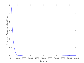
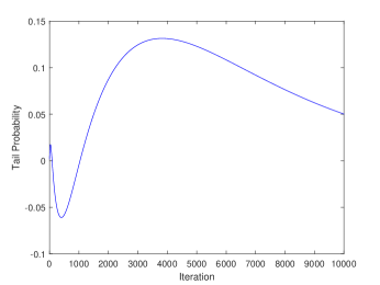
Figure 1: Simulation results of the difference of EAEs and TPs for the artificial case.

7.2 Numerical comparison for the Two EAs on Deceptive

Now we turn to discuss $(1+1)EA$ and $(1+1)EA_{C}$ on Deceptive. We demonstrate $(1+1)EA_{C}$ may not outperform $(1+1)EA$ over all generations although the transition matrix of $(1+1)EA_{C}$ dominates that of $(1+1)EA$.

Example 5

In $(1+1)EA$ and $(1+1)EA_{C}$, set

$$p_{m}=C_{R}q_{m}=\frac{1}{n}.$$

For $(1+1)EA_{C}$, let $q_{m}=\frac{1}{2}$, $C_{R}=\frac{2}{n}$. The numerical simulation results of EAEs and TPS for 5000 independent runs are depicted in Figure 2. It is shown that when $n\geq 9$, both EAEs and TPS of $(1+1)EA$ could be smaller than those of $(1+1)EA_{C}$. This indicates that the dominance of transition matrix does not always guarantee the outperformance of the corresponding algorithm.

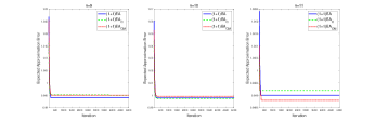
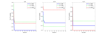
Figure 2: Numerical comparison on expected approximation errors (EAEs) and tail probabilities (TPs) of $(1+1)EA$ and $(1+1)EA_{C}$ applied to the Deceptive problem, where $n$ refers to the problem dimension.

With $p_{m}=C_{R}q_{m}=p\leq\frac{1}{n}$, although the binomial crossover leads to transition dominance of the $(1+1)EA_{C}$ over the $(1+1)EA$, the enhancement of exploitation plays a governing role in the iteration process. Thus, the imbalance of exploration and exploitation leads to a poor performance of $(1+1)EA_{C}$ on some stage of the iteration process.

7.3 Comparisons on the Probabilities to Transfer from Non-optimal Statuses to the Optimal Status

As shown in the previous two counterexamples, the outperformance of $(1+1)EA){MC}$ cannot be drawn from dominance of transition matrices. To enhance the performance of an EA, adaptive parameter settings should be incorporated to improve the exploration ability of an EA on Deceptive.

Local exploitation could result in convergence to the local optimal solution, global convergence of EAs on Deceptive is principally attributed to the direct transition from level $j$ to level $0$, which is quantified by the transition probability $r_{0,j}$. Thus, we investigate the impact of binomial crossover on the transition probability $r_{0,j}$, and accordingly, arrive at the strategies for adaptive regulations of the mutation rate and the crossover rate.

In the following, we first compare $p_{0,j}$ and $s_{0,j}$ by investigating their monotonicity, and then, get reasonable adaptive strategies that improve the performance of EAs on the Deceptive problem.

Substituting (13) and (14) to (25) and (26), respectively, we have

$$p_{0,j}=P_{1}(n-j+1,p_{m})=(p_{m})^{n-j+1}(1-p_{m})^{j-1},$$ (47)

$$s_{0,j}=P_{3}(n-j+1,C_{R},q_{m})$$

$$=\frac{1}{n}\left[(j-1)(1-C_{R})+nC_{R}(1-q_{m})\right]C_{R}^{n-j}(q_{m})^{n-j+1}\left(1-q_{m}C_{R}\right)^{j-2}.$$ (48)

We first investigate the maximum values of $p_{0,j}$ to get the ideal performance of $(1+1)EA$ on the Deceptive problem.

Theorem 5

While

$$p^{\star}_{m}=\frac{n-j+1}{n},$$ (49)

$p_{0,j}$ gets its maximum values

$$p_{0,j}^{max}=\left(\frac{n-j+1}{n}\right)^{n-j+1}\left(\frac{j-1}{n}\right)^{j-1}.$$ (50)

Proof  By (47), we know

$${\frac{\partial}{\partial(p_{m})}p_{0,j}=(n-j+1-np_{m})p_{m}^{n-j}\left(1-p_{m}\right)^{j-2}}.$$

While $p_{m}=\frac{n-j+1}{n}$, $p_{0,j}$ gets its maximum value

$$p_{0,j}^{max}=P_{1}(n-j+1,\frac{n-j+1}{n})=\left(\frac{n-j+1}{n}\right)^{n-j+1}\left(\frac{j-1}{n}\right)^{j-1}.$$

$\square$

Influence of the binomial crossover on $s_{0,j}$ is investigated on condition that $p_{m}=q_{m}$. By regulating the crossover rate $C_{R}$, we can compare $p_{0,j}$ with the maximum value $s_{0,j}^{max}$ of $s_{0,j}$.

Theorem 6

On condition that $p_{m}=q_{m}$, the following results hold.

1. $p_{0,1}=s^{max}_{0,1}$.

2. If $q_{m}>\frac{n-1}{n}$, $p_{0,2}<s^{max}_{0,2}$; otherwise, $p_{0,2}=s^{max}_{0,2}$.

3. $\forall\,\,j\in\{3,\dots,n-1\}$, $p_{0,j}\leq s^{max}_{0,j}$ if $q_{m}>\frac{n-j}{n-1}$; otherwise, $s^{max}_{0,j}=p_{0,j}$.

4. if $q_{m}>\frac{1}{n}$, $p_{0,n}<s^{max}_{0,n}$; otherwise, $s^{max}_{0,n}=p_{0,n}$.

Proof  Note that $(1+1)EA_{C}$ degrades to $(1+1)EA$ when $C_{R}=1$. Then, if the maximum value $s_{0,j}^{max}$ of $s_{0,j}$ is obtained by setting $C_{R}=1$, we have $s_{0,j}^{max}=p_{0,j}$; otherwise, it holds $s_{0,j}^{max}>p_{0,j}$.

1. For the case that $\boldsymbol{j=1}$, equation (48) implies

   $${{s}_{0,1}}=q_{m}^{n}{{\left(C_{R}\right)}^{n-1}}.$$

   Obviously, $s_{0,1}$ is monotonously increasing in $C_{R}$. It gets the maximum value while $C_{R}^{\star}=1$. Then, by (47) we have $s^{max}_{0,1}=p_{0,1}$.

2. While $\boldsymbol{j=2}$, by (48) we have

   $$\frac{\partial s_{0,2}}{\partial C_{R}}=\frac{n-1}{n}q_{m}^{n-1}{{\left(C_{R}\right)}^{n-3}}\left(n-2\text{+}\left(1-n{{q}_{m}}\right)C_{R}\right).$$

   • If $0<{{q}_{m}}\leq\frac{n-1}{n}$, ${s}_{0,2}$ is monotonously increasing in $C_{R}$, and gets its maximum value while $C_{R}^{\star}=1$. For this case, we know $s^{max}_{0,2}=p_{0,2}$.

   • While $\frac{n-1}{n}<{q}_{m}<1$, ${s}_{0,2}$ gets its maximum value $s_{0,2}^{max}$ by setting

     $$C_{R}^{\star}=\frac{n-2}{nq_{m}-1}.$$ (51)

     Then, we have $s_{0,2}^{max}>p_{0,2}$.

3. For the case that $\boldsymbol{3\leq j\leq n-1}$, we denote

   $${s}_{0,j}=\frac{n-j+1}{n}q_{m}^{n-j+1}I_{1}+\frac{\left(j-1\right)\left(1-{{q}_{m}}\right)}{n}q_{m}^{n-j+1}I_{2},$$

   where

   $$I_{1}={{\left(C_{R}\right)}^{n-j}}{{\left(1-{{q}_{m}}C_{R}\right)}^{j-1}},$$

   $$I_{2}={{\left(C_{R}\right)}^{n-j+1}}{{\left(1-{{q}_{m}}C_{R}\right)}^{j-2}}.$$

   Then,

   $$\frac{\partial I_{1}}{\partial C_{R}}={{\left(C_{R}\right)}^{n-j-1}}{{\left(1-{{q}_{m}}C_{R}\right)}^{j-2}}\left(n-j-\left(n-1\right){{q}_{m}}C_{R}\right),$$

   $$\frac{\partial I_{2}}{\partial C_{R}}={{\left(C_{R}\right)}^{n-j}}{{\left(1-\frac{C_{R}}{n}\right)}^{j-3}}\left(n-j+1-\left(n-1\right){{q}_{m}}C_{R}\right).$$

   • While $0<q_{m}\leq\frac{n-j}{n-1}$, both $I_{1}$ and $I_{2}$ are monotonously increasing in $C_{R}$. For this case, $s_{0,j}$ gets its maximum value when $C_{R}^{\star}=1$, and we have $s^{max}_{0,j}=p_{0,j}$.

   • If $\frac{n-j+1}{n-1}\leq q_{m}\leq 1$, $I_{1}$ gets its maximum value when $C_{R}=\frac{n-j}{(n-1)q_{m}}$, and $I_{2}$ gets its maximum value when $C_{R}=\frac{n-j+1}{(n-1)q_{m}}$. Then, $s_{0,j}$ could get its maximum value $s_{0,j}^{max}$ at some

     $$F^{\star}_{R}\in\left(\frac{n-j}{(n-1)q_{m}},\frac{n-j+1}{(n-1)q_{m}}\right).$$ (52)

     Then, we kmow $s^{max}_{0,j}>p_{0,j}$.

   • If $\frac{n-j}{n-1}<q_{m}<\frac{n-j+1}{n-1}$, $I_{1}$ gets its maximum value when $C_{R}=\frac{n-j}{(n-1)q_{m}}$, and $I_{2}$ is monotonously increasing in $C_{R}$. Then, $s_{0,j}$ could get its maximum value $s_{0,j}^{max}$ at some

     $$F^{\star}_{R}\in\left(\frac{n-j}{(n-1)q_{m}},1\right].$$ (53)

     Then, $s_{0,j}^{max}>p_{0,j}$.

4. While $\boldsymbol{j=n}$, equation (48) implies that

   $$\frac{\partial s_{0,n}}{\partial C_{R}}=\left(n-1\right){{\left(1-{{q}_{m}}C_{R}\right)}^{n-3}}\left(1-2{{q}_{m}}-\left(n-1-n{{q}_{m}}\right){{q}_{m}}C_{R}\right).$$

   Denoting

   $$g\left(q_{m},C_{R}\right)=1-2{{q}_{m}}-\left(n-1-n{{q}_{m}}\right){{q}_{m}}C_{R},$$

   we can confirm the sign of ${\partial s_{0,n}}/{\partial C_{R}}$ by considering

   $$\frac{\partial}{\partial C_{R}}g\left(q_{m},C_{R}\right)=-\left(n-1-n{{q}_{m}}\right){{q}_{m}}.$$

   • While $0<{{q}_{m}}\leq\frac{n-1}{n}$, $g\left(q_{m},C_{R}\right)$ is monotonously decreasing in $C_{R}$, and its minimum value is

     $$g\left(q_{m},1\right)=\left(n{{q}_{m}}-1\right)\left({{q}_{m}}-1\right).$$

     The maximum value of $g\left(q_{m},C_{R}\right)$ is

     $$g\left(q_{m},0\right)=1-2q_{m}.$$

     1. If $0<{{q}_{m}}\leq\frac{1}{n}$, we have

        $$g\left(q_{m},C_{R}\right)\geq g\left(q_{m},1\right)>0.$$

        Thus, $\frac{\partial s_{0,n}}{\partial C_{R}}\geq 0$, and ${{s}_{0,n}}$ is monotonously increasing in $C_{R}$. For this case, $s_{0,n}$ get its maximum value when $C_{R}^{\star}=1$, and we have $s_{0,n}^{max}=p_{0,n}$.

     2. If $\frac{1}{n}<{{q}_{m}}\leq\frac{1}{2}$, ${{s}_{0,n}}$ gets the maximum value $s_{0,n}^{max}$ when

        $$C_{R}^{\star}=\frac{1-2q_{m}}{q_{m}(n-1-nq_{m})}.$$

        Thus, $s_{0,n}^{max}>p_{0,n}$.

     3. If $\frac{1}{2}<{{q}_{m}}\leq\frac{n-1}{n}$, $g\left(q_{m},0\right)<0$, and then, ${{s}_{0,n}}$ is monotonously decreasing in $C_{R}$. Then, its maximum value is obtained by setting $C_{R}^{\star}=0$. Then, we know $s^{max}_{0,n}>p_{0,n}$.

   • While $\frac{n-1}{n}<{{q}_{m}}\leq 1$, $g\left(q_{m},C_{R}\right)$ is monotonously increasing in $C_{R}$, and its maximum value

     $$g\left(q_{m},1\right)=\left(n{{q}_{m}}-1\right)\left({{q}_{m}}-1\right)<0.$$

     Then, ${{s}_{0,n}}$ is monotonously decreasing in $C_{R}$, and its maximum value is obtained by setting $C_{R}^{\star}=0$. Then, $s^{max}_{0,n}>p_{0,n}$.

   In summary, $s^{max}_{0,n}>p_{0,n}$ while $q_{m}>\frac{1}{n}$; otherwise, $s^{max}_{0,n}=p_{0,n}$.

$\square$

Theorems 5 and 6 presents the “best” settings to maximize the transition probabilities from non-optimal statues to the optimal level. Unfortunately, such results are not available if the global optima solution is unknown.

7.4 Parameter Adaptive Strategy to Enhance Exploration of EAs

We proposes a parameter Adaptive Strategy based on Hamming distance. Since the level index $j$ is equal to the Hamming distance between $\mathbf{x}$ and $\mathbf{x}^{*}$, improvement of level index $j$ is in deed equal to reduction of the Hamming distance obtained by replacing $\mathbf{x}$ with $\mathbf{y}$. Then, while the local exploitation leads to transition from level $j$ to a non-optimal level $i$, the practically adaptive strategy of parameters can be obtained according to the Hamming distance between $\mathbf{x}$ and $\mathbf{y}$.

For the Deceptive problem, consider two solutions $\mathbf{x}$ and $\mathbf{y}$ such that $f(\mathbf{y})>f(\mathbf{x})$, and denote their levels by $j$ and $i$, respectively. When the $(1+1)EA$ is located at the solution $\mathbf{x}$, equation (49) implies that the “best” setting of mutation rate is $p^{\star}_{m}=\frac{n-j+1}{n}$. While the promising solution $\mathbf{y}$ is generated, the level transfers from $j$ to $i$, and the “best” setting change to $p^{\star}_{m}=\frac{n-i+1}{n}$. Let $H(\mathbf{x},\mathbf{y})$ denote the Hamming distance between $\mathbf{x}$ and $\mathbf{y}$. Noting that $H(\mathbf{x},\mathbf{y})\geq j-i$, we know the difference of “best” parameter settings is bounded from above by $\frac{H(\mathbf{x},\mathbf{y})}{n}$. Accordingly, the mutation rate of $(1+1)EA$ can be updated to

$$p^{\prime}_{m}=p_{m}+\frac{H(\mathbf{x},\mathbf{y})}{n}.$$ (54)

For the $(1+1)EA_{C}$, the parameter $q_{m}$ is adapted using the strategy consistent to that of $p_{m}$ to focus on influence of $C_{R}$. That is,

$$q^{\prime}_{m}=q_{m}+\frac{H(\mathbf{x},\mathbf{y})}{n}.$$ (55)

Since $s_{0,j}$ demonstrates different monotonicity for varied levels, one cannot get an identical strategy for adaptive setting of $C_{R}$. As a compromise, we would like to consider the case that $3\leq j\leq n-1$, which is obtained by random initialization with overwhelming probability.

According to the proof of Theorem 6, we know $C_{R}$ should be set as great as possible for the case $q_{m}\in(0,\frac{n-j}{n-1}]$; while $q_{m}\in(\frac{n-j}{n-1},1]$, $C_{R}^{\star}$ is located in intervals whose boundary values are $\frac{n-j}{(n-1)q_{m}}$ and $\frac{n-j+1}{(n-1)q_{m}}$, given by (52) and (53), respectively. Then, while $q_{m}$ is updated by (55), the update strategy of $C_{R}$ can be confirmed to satisfying that

$$F^{\prime}_{R}q^{\prime}_{m}=C_{R}q_{m}+\frac{H(\mathbf{x},\mathbf{y})}{n-1}.$$

Accordingly, the adaptive setting of $C_{R}$ could be

$$F^{\prime}_{R}=\left(C_{R}q_{m}+\frac{H(\mathbf{x},\mathbf{y})}{n-1}\right)/q^{\prime}_{m},$$ (56)

where $q^{\prime}_{m}$ is updated by (55).

To demonstrate the promising function of the adaptive update strategy, we incorporate it to $(1+1)EA$ and $(1+1)EA_{C}$ to get the adaptive variant of these algorithms, and test their performance on the 12-20 dimensional Deceptive problems. Parameters of EAs are initialized by (15), and adapted according to (54), (55) and (56), respectively.

Since the adaptive strategy decreases stability of performances to a large extent, numerical simulation of the tail probability is implemented by 10,000 independent runs. To investigate the sensitivity of the adaptive strategy on initial values of $q_{m}$, the mutation rate $q_{m}$ in $(1+1)EA_{C}$ is initialized with values $\frac{1}{\sqrt{n}}$, $\frac{3}{2\sqrt{n}}$ and $\frac{2}{\sqrt{n}}$, where the three variants are denoted by $(1+1)EA_{C}^{1}$, $(1+1)EA_{C}^{2}$ and $(1+1)EA_{C}^{3}$, respectively.

The converging curves of averaged TPs are illustrated in Figure 3. Compared to the EAs with fixed parameters during the evolution process, the performance of adaptive EAs has significantly been improved. Meanwhile, the outperformance of $(1+1)EA_{C}$ introduced by the binomial crossover is greatly enhanced by the adaptive strategies, too.

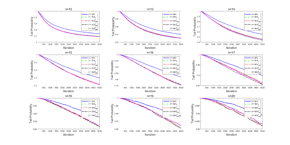
Figure 3: Numerical comparison on tail probabilities (TPs) of adaptive $(1+1)EA$, $(1+1)EA_{C}$ and $(1+1)EA_{C}$ applied to the Deceptive problem, where $n$ is the problem dimension. The $(1+1)EA_{C}^{1}$, $(1+1)EA_{C}^{2}$ and $(1+1)EA_{C}^{3}$ are three variants of $(1+1)EA_{C}$ with $q_{m}$ initialized as $\frac{1}{\sqrt{n}}$, $\frac{3}{2\sqrt{n}}$ and $\frac{2}{\sqrt{n}}$, respectively.

8 Conclusions

Under the framework of fixed budget analysis, we conduct a pioneering analysis of the influence of binomial crossover on the approximation error of EAs. The performance of an EA after running finite generations is measured by two metrics: the expected value of the approximation error and the error tail probability. Using the two metrics, we make a case study of comparing the approximation error of $(1+1)EA$ and $(1+1)EA_{C}$ with binomial crossover.

Starting from the comparison on probability of flipping “l preferred bits”, it is proven that under proper conditions, incorporation of binomial crossover leads to dominance of transition probabilities, that is, the probability of transferring to any promising status is improved. Accordingly, the asymptotic performance of $(1+1)EA_{C}$ is superior to that of $(1+1)EA$.

It is found that the dominance of transition probability guarantees that $(1+1)EA_{C}$ outperforms $(1+1)EA$ on OneMax in terms of both expected approximation error and tail probability. However, this dominance does leads to the outperformance on Deceptive. This means that using binomial crossover may reduce the approximation error on some problems but not on other problems.

For Deceptive, an adaptive strategy of parameter setting is proposed based on the monotonicity analysis of transition probabilities. Numerical simulations demonstrate that it can significantly improve the exploration ability of $(1+1)EA_{C}$ and $(1+1)EA$, and superiority of binomial crossover is further strengthened by the adaptive strategy. Thus, a problem-specific adaptive strategy is helpful for improving the performance of EAs.

Our future work will focus on a further study for adaptive setting of crossover rate in population-based EAs on more complex problems, as well as development of adaptive EAs improved by introduction of binomial crossover.

References

- [1] T. Jansen, I. Wegener, et al., The analysis of evolutionary algorithms–a proof that crossover really can help, Algorithmica 34 (1) (2002) 47–66.
- [2] T. Kötzing, D. Sudholt, M. Theile, How crossover helps in pseudo-boolean optimization, in: Proceedings of the 13th annual conference on Genetic and evolutionary computation, 2011, pp. 989–996.
- [3] D. Corus, P. S. Oliveto, Standard steady state genetic algorithms can hillclimb faster than mutation-only evolutionary algorithms, IEEE Transactions on Evolutionary Computation 22 (5) (2017) 720–732.
- [4] D.-C. Dang, T. Friedrich, T. Kötzing, M. S. Krejca, P. K. Lehre, P. S. Oliveto, D. Sudholt, A. M. Sutton, Escaping local optima using crossover with emergent diversity, IEEE Transactions on Evolutionary Computation 22 (3) (2017) 484–497.
- [5] D. Sudholt, How crossover speeds up building block assembly in genetic algorithms, Evolutionary computation 25 (2) (2017) 237–274.
- [6] E. C. Pinto, C. Doerr, A simple proof for the usefulness of crossover in black-box optimization, in: International Conference on Parallel Problem Solving from Nature, Springer, 2018, pp. 29–41.
- [7] P. S. Oliveto, D. Sudholt, C. Witt, A tight lower bound on the expected runtime of standard steady state genetic algorithms, in: Proceedings of the 2020 Genetic and Evolutionary Computation Conference, 2020, pp. 1323–1331.
- [8] J. Lengler, J. Meier, Large population sizes and crossover help in dynamic environments, in: International Conference on Parallel Problem Solving from Nature, Springer, 2020, pp. 610–622.
- [9] P. K. Lehre, X. Yao, Crossover can be constructive when computing unique input output sequences, in: Asia-Pacific Conference on Simulated Evolution and Learning, Springer, 2008, pp. 595–604.
- [10] B. Doerr, E. Happ, C. Klein, Crossover can provably be useful in evolutionary computation, Theoretical Computer Science 425 (2012) 17–33.
- [11] B. Doerr, D. Johannsen, T. Kötzing, F. Neumann, M. Theile, More effective crossover operators for the all-pairs shortest path problem, Theoretical Computer Science 471 (2013) 12–26.
- [12] A. M. Sutton, Fixed-parameter tractability of crossover: Steady-state gas on the closest string problem, Algorithmica 83 (4) (2021) 1138–1163.
- [13] J. N. Richter, A. Wright, J. Paxton, Ignoble trails-where crossover is provably harmful, in: International Conference on Parallel Problem Solving from Nature, Springer, 2008, pp. 92–101.
- [14] D. Antipov, S. Naumov, The effect of non-symmetric fitness: the analysis of crossover-based algorithms on realjump functions, in: Proceedings of the 16th ACM/SIGEVO Conference on Foundations of Genetic Algorithms, 2021, pp. 1–15.
- [15] S. Das, P. N. Suganthan, Differential evolution: A survey of the state-of-the-art, IEEE Transactions on Evolutionary Computation 15 (1) (2011) 4–31. doi:10.1109/TEVC.2010.2059031.
- [16] S. Das, S. S. Mullick, P. Suganthan, Recent advances in differential evolution – an updated survey, Swarm and Evolutionary Computation 27 (2016) 1–30. doi:https://doi.org/10.1016/j.swevo.2016.01.004.
- [17] M. Sepesy Maučec, J. Brest, A review of the recent use of differential evolution for large-scale global optimization: An analysis of selected algorithms on the cec 2013 lsgo benchmark suite, Swarm and Evolutionary Computation 50 (2019) 100428. doi:https://doi.org/10.1016/j.swevo.2018.08.005.
-
[18]
Bilal, M. Pant, H. Zaheer, L. Garcia-Hernandez, A. Abraham,