The Block-Correlated Pseudo Marginal Sampler for State Space Models

Abstract

Particle Marginal Metropolis-Hastings (PMMH) is a general approach to Bayesian inference when the likelihood is intractable, but can be estimated unbiasedly. Our article develops an efficient PMMH method that scales up better to higher dimensional state vectors than previous approaches. The improvement is achieved by the following innovations. First, the trimmed mean of the unbiased likelihood estimates of the multiple particle filters is used. Second, a novel block version of PMMH that works with multiple particle filters is proposed. Third, the article develops an efficient auxiliary disturbance particle filter, which is necessary when the bootstrap disturbance filter is inefficient, but the state transition density cannot be expressed in closed form. Fourth, a novel sorting algorithm, which is as effective as previous approaches but significantly faster than them, is developed to preserve the correlation between the logs of the likelihood estimates at the current and proposed parameter values. The performance of the sampler is investigated empirically by applying it to non-linear Dynamic Stochastic General Equilibrium models with relatively high state dimensions and with intractable state transition densities and to multivariate stochastic volatility in the mean models. Although our focus is on applying the method to state space models, the approach will be useful in a wide range of applications such as large panel data models and stochastic differential equation models with mixed effects.

Keywords: Block PMMH; correlated PMMH; dynamic stochastic general equilibrium (DSGE) model; trimmed mean likelihood estimate

1 Introduction

Particle marginal Metropolis-Hastings (PMMH) (Andrieu and Roberts, , 2009) is a Bayesian inference method for statistical models having an intractable likelihood, when the likelihood can be estimated unbiasedly. Our article develops a PMMH sampling method for efficiently estimating the parameters of complex state space models. The method scales better than current approaches in the number of observations and latent states and can handle state transition densities that cannot be expressed in closed form; e.g., many dynamic stochastic general equilibrium (DSGE) models, which are a popular class of macroeconomic time series state space models, do not have closed form transition densities.

A key issue in efficiently estimating statistical models using a PMMH approach is that the variance of the log of the estimated likelihood grows with the number of observations and the dimension of the latent states (Deligiannidis et al., , 2018). Pitt et al., (2012) show that to obtain a balance between computational time and the mixing of the Markov chain Monte Carlo (MCMC) chain, the number of particles used in the particle filter should be such that the variance of the log of the estimated likelihood is in the range 1 to 3, depending on the efficiency of the proposal for $\theta$. Pitt et al., (2012) also show that the efficiency of PMMH schemes deteriorates exponentially as that variance increases; we further note that in many complex statistical applications, it is computationally very expensive ensuring that the variance of the log of the estimated likelihood is within the required range.

Deligiannidis et al., (2018) propose a more efficient PMMH scheme, called the correlated pseudo-marginal (CPM) method, which correlates the random numbers in the (single) particle filters used to construct the estimated likelihoods at the current and proposed values of the parameters. This dependence induces a positive correlation between the estimated likelihoods and reduces the variance of the difference in the logs of the estimated likelihoods which appear in the Metropolis-Hastings (MH) acceptance ratio. They show that the CPM scales up with the number of observations compared to the standard pseudo marginal method of Andrieu et al., (2010) when the state dimension is small.

Tran et al., (2016) propose an alternative correlated pseudo marginal approach to that of Deligiannidis et al., , calling it the block pseudo marginal (BPM) method; the BPM divides the random numbers used in constructing likelihood estimators into blocks and then updates the parameters jointly with one randomly chosen block of the random numbers in each MCMC iteration; this induces a positive correlation between the numerator and denominator of the MH acceptance ratio, similarly to the CPM. They show that for large samples the correlation of the logs of the estimated likelihoods at the current and proposed values is close to $1-1/S$, where $S$ is the number of blocks. However, they do not apply the BPM method for estimating time series state space models using the particle filter.

Our article introduces a new PMMH sampler, referred to as the multiple PMMH algorithm (MPM), which extends the CPM method of Deligiannidis (2018) and the BPM method of Tran (2016). The MPM sampler is innovative and addresses various issues in the following ways: (a) The likelihood estimator is a trimmed mean of unbiased likelihood estimators from multiple independent particle filters (PFs); these PFs can be run in parallel. This approach reduces the variance of the likelihood estimator compared to using a single particle filter. The algorithm is exact when there is no trimming and approximate otherwise, but our empirical results suggest that the approximation is very close to being exact. (b) The unknown parameters, and only the random numbers used in one of the PFs, are updated jointly. This is a novel block version of PMMH that works with multiple particle filters. See section 2.3 for details. (c) An auxiliary disturbance PF (ADPF) algorithm is proposed to estimate the likelihood efficiently for state space models such as DSGE models, where the bootstrap filter is very inefficient and the state transition density does not have a closed form so that an auxiliary PF cannot be constructed; see section 2.5 for details. (d) A novel sorting algorithm, which is as effective as previous approaches but is significantly faster than them, is proposed to maintain the correlation between the logs of the likelihood estimates at the current and proposed values. The standard resampling step in the particle filter introduces discontinuities that break down the correlation between the logs of the likelihood estimates at the current and proposed values, even when the current and proposed parameters are close. Section 3.2 shows that the MPM sampler with the proposed sorting algorithm can maintain the correlation between the logs of the estimated likelihoods for relatively high dimensional state space models. Note that the proposed PMMH sampler works with any particle filter algorithm, including the tempered particle filter of Herbst and Schorfheide, (2019), the standard bootstrap filter of Gordon et al., (1993), the disturbance particle filter of Murray et al., (2013), and the proposed auxiliary disturbance filter. When the number of state dimensions is greater than the number of disturbance dimensions, a disturbance particle filter is more efficient than a state-based particle filter. Additionally, the disturbance particle filter is useful for state space models with intractable state transition density.

We illustrate the MPM sampler empirically, and compare its performance to the CPM method, using a standard linear Gaussian state space model, a multivariate stochastic volatility in the mean model and two non-linear Dynamic Stochastic General Equilibrium (DSGE) models, using simulated and real data. Our work in estimating non-linear DSGE models is also related to Fernández-Villaverde and Rubio-Ramírez, (2007) and Hall et al., (2014) who use standard PMMH methods. We note that the MPM sampler will also be useful for other complex statistical models, such as panel data models and stochastic differential equation mixed effects models.

The rest of the article is organised as follows. Section 2 introduces the state space model and gives some examples. Section 2.3 discusses the MPM sampler. Section 3 presents results from both simulated and real data. Section 4 concludes with a discussion of our major results and findings. The paper has an online supplement containing some further technical and empirical results.

2 Bayesian Inference for State Space Models

Notation

We use the colon notation for collections of variables, i.e., $a_{t}^{r:s}:=\left(a_{t}^{r},...,a_{t}^{s}\right)$ and for $t\leq u$, $a_{t:u}^{r:s}:=\left(a_{t}^{r:s},...,a_{u}^{r:s}\right)$. Suppose $\left\{\left(Z_{t},Y_{t}\right),t\geq 0\right\}$ is a stochastic process, with parameter $\theta$, where the $Y_{t}$ are the observations and the $Z_{t}$ are the latent state vectors; random variables are denoted by capital letters and their realizations by lower case letters. We consider the state space model with $p\left(z_{0}|\theta\right)$ the density of $Z_{0},$ $p\left(z_{t}|z_{t-1},\theta\right)$ the density of $Z_{t}$ given $Z_{0:t-1}=z_{0:t-1}$ for $t\geq 1$, and $p\left(y_{t}|z_{t},\theta\right)$ is the density of $Y_{t}$ given $Z_{0:t}=z_{0:t}$, $Y_{1:t-1}=y_{1:t-1}$.

2.1 Bayesian Inference

The objective of Bayesian inference is to obtain the posterior distribution of the model parameters $\theta$ and the latent states $z_{0:T}$, given the observations $y_{1:T}$ and a prior distribution $p\left(\theta\right)$; i.e.,

$$p\left(\theta,z_{0:T}|y_{1:T}\right) = p\left(y_{1:T}|\theta,z_{0:T}\right)p\left(z_{0:T}|\theta\right)p\left(\theta\right)/p\left(y_{1:T}\right),$$ (1)

where

$$p\left(y_{1:T}\right)=\int\int p\left(y_{1:T}|\theta,z_{0:T}\right)p\left(z_{0:T}|\theta\right)p\left(\theta\right)dz_{0:T}d\theta$$

is the marginal likelihood. The likelihood

$$p\left(y_{1:T}|\theta\right)=\int p\left(y_{1:T}|\theta,z_{0:T}\right)p\left(z_{0:T}|\theta\right)dz_{0:T}$$

can be calculated exactly using the Kalman filter for linear Gaussian state space models (LGSS) and for linear DSGE models so that posterior samples can be obtained using an MCMC sampling scheme. However, the likelihood can be estimated unbiasedly, but not computed exactly, for non-linear and non-Gaussian state space models and the non-linear DSGE models described in section 3.4.

The bootstrap particle filter (Gordon et al., , 1993) provides an unbiased estimator of the likelihood for a general state space model. Andrieu and Roberts, (2009) and Andrieu et al., (2010) show that it is possible to use this unbiased estimator of the likelihood to carry out exact Bayesian inference for the parameters of the general state space model. They call this MCMC approach pseudo marginal Metropolis-Hastings (PMMH).

The non-linear (second-order) DSGE models considered in section 3.4 lie within the class of general non-linear state space models whose state transition density is difficult to work with or cannot be expressed in closed form. In such cases, it is useful to express the model in terms of the density of its latent disturbance variables as it can be expressed in closed form. The posterior in Eq. (1) becomes

$$p\left(\theta,\epsilon_{1:T},z_{0}|y_{1:T}\right)\propto\prod_{t=1}^{T}p\left(y_{t}|\epsilon_{1:t},\theta,z_{0}\right)p\left(\epsilon_{t}\right)p\left(z_{0}|\theta\right)p\left(\theta\right),$$ (2)

which Murray et al., (2013) call the disturbance state-space model. The standard state space model can be recovered from the disturbance state space model by using the deterministic function $F\left(z_{t-1},\epsilon_{t};\theta\right)\rightarrow z_{t}$. This gives us a state trajectory $z_{0:T}$ from any sample $\left(\epsilon_{1:T},z_{0}\right)$. In the disturbance state-space model the target becomes the posterior distribution over the parameters $\theta$, the latent noise variables $\epsilon_{1:T}$ and the initial state $z_{0}$, rather than $\left(\theta,z_{0:T}\right)$.

2.2 Standard Pseudo Marginal Metropolis-Hastings

This section outlines the standard PMMH scheme which carries out MCMC on an expanded space using an unbiased estimate of the likelihood. Our paper focuses on MCMC based on the parameters, but it is straightforward to also use it to obtain posterior inference for the unobserved states; see, e.g., Andrieu et al., (2010). Let $u$ consist of all the random variables required to compute the unbiased likelihood estimate $\widehat{p}_{N}\left(y|\theta,u\right)$, with $p(u)$ the density of $u$; let $p\left(\theta\right)$ be the prior of $\theta$. The joint posterior density $\theta$ and $u$ is

$$p\left(\theta,u|y_{1:T}\right)=\widehat{p}_{N}\left(y_{1:T}|\theta,u\right)p\left(\theta\right)p\left(u\right)/p\left(y_{1:T}\right),$$

so that

$$p\left(\theta|y_{1:T}\right)=\int p\left(\theta,u|y_{1:T}\right)du=p\left(y_{1:T}|\theta\right)p\left(\theta\right)/p\left(y_{1:T}\right)$$

is the posterior of $\theta$ and $\intop\widehat{p}_{N}\left(y_{1:T}|\theta,u\right)p\left(u\right)du=p\left(y_{1:T}|\theta\right)$ because the likelihood estimate is unbiased. We can therefore sample from the posterior density $p\left(\theta|y_{1:T}\right)$ by sampling $\theta$ and $u$ from $p\left(\theta,u|y_{1:T}\right)$. The subscript $N$ indicates the number of particles used to estimate the likelihood.

Let $q\left(\theta^{{}^{\prime}}|\theta\right)$ be the proposal density for $\theta^{\prime}$ with the current value $\theta$ and $q\left(u^{{}^{\prime}}|u\right)$ the proposal density for $u^{{}^{\prime}}$ given $u$. We always assume that $q\left(u^{{}^{\prime}}|u\right)$ satisfies the reversibility condition

$$q\left(u^{{}^{\prime}}|u\right)p\left(u\right)=q\left(u|u^{{}^{\prime}}\right)p\left(u^{{}^{\prime}}\right);$$

it is clearly satisfied by the standard PMMH where $q\left(u^{{}^{\prime}}|u\right)=p\left(u^{{}^{\prime}}\right)$. We generate a proposal $\theta^{{}^{\prime}}$ from $q\left(\theta^{{}^{\prime}}|\theta\right)$ and $u^{{}^{\prime}}$ from $q\left(u^{{}^{\prime}}|u\right)$, and accept both proposals with probability

$$\alpha\left(\theta,u;\theta^{{}^{\prime}},u^{{}^{\prime}}\right) = \min\left(1,\frac{\widehat{p}_{N}\left(y|\theta^{{}^{\prime}},u^{{}^{\prime}}\right)p\left(\theta^{{}^{\prime}}\right)p\left(u^{{}^{\prime}}\right)q\left(\theta|\theta^{{}^{\prime}}\right)q\left(u|u^{{}^{\prime}}\right)}{\widehat{p}_{N}\left(y|\theta,u\right)p\left(\theta\right)p\left(u\right)q\left(\theta^{{}^{\prime}}|\theta\right)q\left(u^{{}^{\prime}}|u\right)}\right)$$ (3)

$$= \min\left(1,\frac{\widehat{p}_{N}\left(y|\theta^{{}^{\prime}},u^{{}^{\prime}}\right)p\left(\theta^{{}^{\prime}}\right)q\left(\theta|\theta^{{}^{\prime}}\right)}{\widehat{p}_{N}\left(y|\theta,u\right)p\left(\theta\right)q\left(\theta^{{}^{\prime}}|\theta\right)}\right).$$

The expression in Eq. (3) is identical to a standard Metropolis-Hastings algorithm, except that estimates of the likelihood at the current and proposed parameters are used. Andrieu and Roberts, (2009) show that the resulting PMMH algorithm has the correct invariant distribution regardless of the variance of the estimated likelihoods. However, the performance of the PMMH approach crucially depends on the number of particles $N$ used to estimate the likelihood. The variance of the log of the estimated likelihood should be between 1 and 3 depending on the quality of the proposal for $\theta$; see Pitt et al., (2012) and Sherlock et al., (2015). In many applications of the non-linear state space models considered in this paper, it is computationally very expensive to ensure that the variance of the log of the estimated likelihood is within the required range. Section 2.3 discusses the new PMMH sampler, which we call the multiple PMMH algorithm (MPM), that builds on and extends, the CPM of Deligiannidis et al., (2018) and BPM of Tran et al., (2016).

2.3 Multiple PMMH (MPM)

This section discusses Algorithm 1, which is the proposed multiple PMMH (MPM) method that uses multiple particle filters to obtain the estimate of the likelihood. The novel version of block-correlated PMMH that works with multiple particle filters to induce a high correlation between successive logs of the estimated likelihoods is also discussed. We now define the joint target density of $\theta$ and $\widetilde{u}=\left(u_{1},...,u_{S}\right)$ as

$$p\left(\theta,\widetilde{u}|y_{1:T}\right)\propto\overline{\widehat{p}}_{N}\left(y|\theta,\widetilde{u}\right)p\left(\theta\right)\prod_{s=1}^{S}p\left(u_{s}\right),$$ (4)

where $\overline{\widehat{p}}_{N}\left(y|\theta,u\right)$ is the likelihood estimates obtained from $S$ particle filters discussed below. We update the parameters $\theta$ jointly with a randomly selected block $u_{s}$ in each MCMC iteration, with $\Pr\left(S=s\right)=1/S$ for any $s=1,...,S$. The selected block $u_{s}$ is updated using $u_{s}^{{}^{\prime}}=\rho_{u}u_{s}+\sqrt{1-\rho_{u}^{2}}\eta_{u}$, where $\rho_{u}$ is the non-negative correlation between the random numbers $u_{s}$ and $u_{s}^{{}^{\prime}}$ and $\eta_{u}$ is a standard normal vector of the same length as $u_{s}$. This is similar to component-wise MCMC whose convergence is well established in the literature; see, e.g. Johnson et al., (2013). Using this scheme, the acceptance probability is

$$\alpha\left(\theta,\widetilde{u};\theta^{{}^{\prime}},\widetilde{u}^{{}^{\prime}}\right)=\min\left(1,\frac{\overline{\widehat{p}}_{N}\left(y|\theta^{{}^{\prime}},\widetilde{u}^{{}^{\prime}}=\left(u_{1},...,u_{s-1},u_{s}^{{}^{\prime}},u_{s+1},...,u_{S}\right)\right)p\left(\theta^{{}^{\prime}}\right)q\left(\theta|\theta^{{}^{\prime}}\right)}{\overline{\widehat{p}}_{N}\left(y|\theta,\widetilde{u}=\left(u_{1},...,u_{s-1},u_{s},u_{s+1},...,u_{S}\right)\right)p\left(\theta\right)q\left(\theta^{{}^{\prime}}|\theta\right)}\right).$$ (5)

Algorithm 1 The Multiple PMMH (MPM) algorithm

• Set the initial values of $\theta^{\left(0\right)}$ arbitrarily.

• Sample $u_{s}\sim N\left(0,I\right)$ for $s=1,...,S$, and run $S$ particle filters to estimate the likelihood $\overline{\widehat{p}}_{N}\left(y|\theta,\widetilde{u}\right)$ as the trimmed mean of $\widehat{p}_{N}\left(y|\theta,u_{s}\right),s=1,\dots,S$; a 0% is the mean and a 50% trimmed mean is the median.

• For each MCMC iteration $p$, $p=1,...,P$,

  • Sample $\theta^{{}^{\prime}}$ from the proposal density $q\left(\theta^{{}^{\prime}}|\theta\right)$.

  • Choose index $s$ with probability $1/S$, sample $\eta_{u}\sim N\left(0,I\right)$, and set $u_{s}^{{}^{\prime}}=\rho_{u}u_{s}+\sqrt{1-{\rho_{u}}^{2}}{\eta_{u}}$.

  • Run $S$ particle filters to compute the estimate of likelihood $\overline{\widehat{p}}_{N}\left(y|\theta^{{}^{\prime}},\widetilde{u}^{{}^{\prime}}\right)$.

  • With the probability in Eq. (5), set $\overline{\widehat{p}}\left(y_{1:T}|\theta,\widetilde{u}\right)^{\left(p\right)}=\overline{\widehat{p}}\left(y_{1:T}|\theta^{{}^{\prime}},\widetilde{u}^{{}^{\prime}}\right)$, $\widetilde{u}^{(p)}=\widetilde{u}^{{}^{\prime}}$, and $\theta^{\left(p\right)}=\theta^{{}^{\prime}}$; otherwise, set $\overline{\widehat{p}}\left(y_{1:T}|\theta,\widetilde{u}\right)^{\left(p\right)}=\overline{\widehat{p}}\left(y_{1:T}|\theta,\widetilde{u}\right)^{\left(p-1\right)}$, $\widetilde{u}^{(p)}=\widetilde{u}^{(p-1)}$, and $\theta^{\left(p\right)}=\theta^{\left(p-1\right)}$.

We now discuss approaches to obtain a likelihood estimate from multiple particle filters which we then use in the MPM algorithm. Suppose that $S$ particle filters are run in parallel. Let $\widehat{p}_{N}\left(y|\theta,u_{s}\right)$ be the unbiased estimate of the likelihood obtained from the $s$th particle filter, for $s=1,...,S$. The first approach takes the average of the $S$ unbiased likelihood estimates from the particle filter. The resulting likelihood estimate

$$\overline{\widehat{p}}_{N}\left(y|\theta,u\right)=\sum_{s=1}^{S}\widehat{p}_{N}\left(y|\theta,u_{s}\right)/S$$ (6)

is also unbiased (Sherlock et al., 2017b, ). The second approach is to take the trimmed mean as the likelihood estimate in MPM. For example, the $20\%$ trimmed mean averages the middle $60\%$ of the likelihood values. Although the trimmed mean does not give an unbiased estimate of the likelihood, we show in section 3 that the posterior based on the trimmed means approximates the exact posterior well.

2.4 Multidimensional Euclidean Sorting Algorithm

It is important that the logs of the likelihood estimates evaluated at the current and proposed values of $\theta$ and $\widetilde{u}$ are highly correlated to reduce the variance of $\log\overline{\widehat{p}}_{N}\left(y|\theta^{{}^{\prime}},\widetilde{u}^{{}^{\prime}}\right)-\log\overline{\widehat{p}}_{N}\left(y|\theta,\widetilde{u}\right)$ because this helps the Markov chain to mix well. However, the standard resampling step in the particle filter introduces discontinuities which breaks down the correlation between the logs of the likelihood estimates at the current and proposed values even when the current parameters $\theta$ and the proposed parameters $\theta^{{}^{\prime}}$ are close. Sorting the particles from smallest to largest before resampling helps to preserve the correlation between the logs of the likelihood estimates at the current and proposed values (Deligiannidis et al., , 2018). However, such simple sorting is unavailable for multidimensional state particles.

This section discusses Algorithm 2, which is the fast multidimensional Euclidean sorting algorithm used to sort the multidimensional state or disturbance particles in the particle filter algorithm described in Algorithm S1 in section S1 of the online supplement. The algorithm is written in terms of state particles, but similar steps can be implemented for the disturbance particles. The algorithm takes the particles $z_{t}^{1:N}$ and the normalised weights $\overline{w}_{t}^{1:N}$ as the inputs; it outputs the sorted particles $\widetilde{z}_{t}^{1:N}$, sorted weights $\widetilde{\overline{w}}_{t}^{1:N}$, and sorted indices $\zeta_{1:N}$. Let $z_{t}^{i}$ be $d$-dimensional particles at a time $t$ for the $i$th particle, $z_{t}^{i}=\left(z_{t,1}^{i},...,z_{t,d}^{i}\right)^{\top}$. Let $d\left(z_{t}^{j},z_{t}^{i}\right)$ be the Euclidean distance between two multidimensional particles. The first step is to calculate the means of the multidimensional particles $\overline{z}_{t}^{i}=(\nicefrac{{1}}{{d}})\sum_{k=1}^{d}z_{t,k}^{i}$ at time $t$ for $i=1,...,N$. The first sorting index, $\zeta_{1}$, is the index of the multidimensional particle having the smallest value of $\overline{z}_{t}^{i}$ for $i=1,...,N$. Therefore, the first sorted particle $\widetilde{z}_{t}^{1}$ is $z_{t}^{\zeta_{1}}$ with its associated weight $\widetilde{\overline{w}}_{t}^{1}=\overline{w}_{t}^{\zeta_{1}}$. We then calculate the Euclidean distance between the selected multidimensional particle and the set of all remaining multidimensional particles, $d\left(\widetilde{z}_{t}^{1},z_{t}^{i}\right)$, for all $i\neq\zeta_{1}$. The next step is to sort the particles and weights according to the Euclidean distance from smallest to largest to obtain the sorted particles $\widetilde{z}_{t}^{2:N}$, sorted weights $\widetilde{\overline{w}}_{t}^{2:N}$, and sorted indices $\zeta_{2:N}$.

Algorithm 2 simplifies the sorting algorithm proposed by Choppala et al., (2016). In Choppala et al., (2016), the first sorting index is the index of the multidimensional particle having the smallest value along its first dimension. To select the second sorted index, $\zeta_{2}$, we need to calculate the Euclidean distance between the first selected particle and the remaining multidimensional particles. Similarly, to select the third sorted index, $\zeta_{3}$, we need to calculate the Euclidean distance between the second selected particle and the remaining multidimensional particles. This process is repeated $N$ times, which is expensive for a large number of particles and long time series. In contrast, Algorithm 2 only needs to calculate the Euclidean distance of the first selected particle and the remaining particles once. Deligiannidis et al., (2018) use the Hilbert sorting method of Skilling, (2004) to order the multidimensional state particles, which requires calculating the Hilbert index for each multidimensional particle and is much more expensive than Algorithm 2. Table 1 shows the CPU time (in seconds) of the three sorting methods for different numbers of particles $N$ and state dimensions $d$. The table shows that the proposed sorting algorithm is much faster than that in Choppala et al., (2016) and the Hilbert sorting method. For example, for state dimensions $d=30$ and $N=2000$ particles, Algorithm 2 is $290$ and $335$ times faster than the Choppala et al., (2016) and the Hilbert sorting methods, respectively

Algorithm 2 Multidimensional Euclidean Sorting Algorithm

Input: $z_{t}^{1:N}$, $\overline{w}_{t}^{1:N}$

Output: sorted particles $\widetilde{z}_{t}^{1:N}$, sorted weights $\widetilde{\overline{w}}_{t}^{1:N}$, sorted indices $\zeta_{1:N}$

• Calculate the means of the multidimensional particles $\overline{z}_{t}^{i}=\frac{1}{d}\sum_{k=1}^{d}z_{t,k}^{i}$ at time $t$ for $i=1,...,N$. The first sorting index, $\zeta_{1}$, is the index of the multidimensional particle having the smallest value of $\overline{z}_{t}^{i}$ for $i=1,...,N$. The first selected particle $\widetilde{z}_{t}^{1}$ is $z_{t}^{\zeta_{1}}$ with its associated weight $\widetilde{\overline{w}}_{t}^{1}=\overline{w}_{t}^{\zeta_{1}}$.

• Calculate the Euclidean distance between the selected multidimensional particle and the set of all remaining multidimensional particles, $d\left(\widetilde{z}_{t}^{1},z_{t}^{i}\right)$, for $\forall i\neq\zeta_{1}$.

• Sort the particles and weights according to the Euclidean distance from smallest to largest to obtain $\zeta_{i}$ for $i=2,...,N$. The sorted particles $\widetilde{z}_{t}^{i}=z_{t}^{\zeta_{i}}$ and $\widetilde{\overline{w}}_{t}^{i}=\overline{w}_{t}^{\zeta_{i}}$ for $i=2,...,N$.

Table 1: Comparing different sorting methods for various combinations of $N$ and $d$ in terms of CPU time (in seconds): I: The fast Euclidean sorting algorithm, II: Choppala et al., (2016) sorting method, and III: Hilbert sorting method. The entries in columns I to III are multiples of the time in column I. The column headed “$I$ actual” is the actual time for column I; e.g. the 30.5 in column II and row 1 means that I is 30.5 times faster than the Choppala et al., (2016) sorting. The corresponding entry for I actual is 0.0002.

$d$	$N$	$I$	$II$	$III$	$I$ actual
10	500	1.00	30.50	87.50	0.0002
	1000	1.00	66.67	115.00	0.0003
	2000	1.00	172.40	141.00	0.0005
30	500	1.00	39.67	141.00	0.0003
	1000	1.00	113.00	214.00	0.0004
	2000	1.00	289.80	335.00	0.0005

2.5 The Auxiliary Disturbance Particle Filter

This section discusses the auxiliary disturbance particle filter we use to obtain the estimates of the likelihood in the MPM sampler described in section 2.3. It is particularly useful for state space models when the state dimension is substantially bigger than the disturbance dimension and the state transition density is intractable. Suppose that $z_{1}=\Phi\left(z_{0},\epsilon_{1};\theta\right)$, where $z_{0}$ is the initial state vector with density $p(z_{0}|\theta)$, and $z_{t}=F\left(z_{t-1},\epsilon_{t};\theta\right)(t\geq 2)$, where $\epsilon_{t}$ is a $n_{e}\times 1$ vector of normally distributed latent noise with density $p\left(\epsilon_{t}\right).$ Murray et al., (2013) express the standard state-space model in terms of the latent noise variables $\epsilon_{1:T}$, and call

$$\epsilon_{t}\sim p\left(\epsilon_{t}\right),y_{t}|\epsilon_{1:t}\sim p\left(y_{t}|\epsilon_{1:t},z_{0};\theta\right)=p\left(y_{t}|z_{t};\theta\right),\,\,t=1,...,T,$$

the disturbance state-space model. We note that the conditional distribution of $y_{t}$ depends on all the latent error variables, $\epsilon_{1:t}.$

We now discuss the proposal for $\epsilon_{t}$ used in the disturbance filter. The defensive mixture proposal density (Hesterberg, , 1995) is

$$m\left(\epsilon_{t}|u_{\epsilon,t},\theta\right)=\pi p\left(\epsilon_{t}|\theta\right)+(1-\pi)q\left(\epsilon_{t}|\theta,y_{1:T}\right),\quad{\rm with}\quad 0<\pi\ll 1,$$ (7)

where $u_{\epsilon,t}$ is the vector random variable used to generate the particles $\epsilon_{t}$ given $\theta$. If the observation density $p\left(y_{t}|z_{t},\theta\right)$ is bounded, then Eq. (7) guarantees that the weights are bounded in the disturbance particle filter algorithm defined in Eq. (S2) of section S1 of the online supplement. In practice, we take $q\left(\epsilon_{t}|\theta,y_{1:T}\right)=N\left(\epsilon_{t}|\widehat{\mu}_{t},\widehat{\Sigma}_{t}\right)$ and set $\pi=0.05$ in all the examples in section 3; see algorithm 4. If $\pi=1$ in Eq. (7), then $m\left(\epsilon_{t}\right)=p\left(\epsilon_{t}\right)$ is the bootstrap disturbance particle filter. However, the empirical performance of this filter is usually poor because the resulting likelihood estimate is too variable.

Algorithm 4 discusses how we obtain $\widehat{\mu}_{t}$ and the covariance matrix $\widehat{\Sigma}_{t}$, for $t=1,...,T$, at each iteration of the MPM algorithm. It is computationally cheap to obtain $\widehat{\mu}_{t}$ and $\widehat{\Sigma}_{t}$ for $t=1,...,T$ because they are obtained from the output of the $S$ disturbance particle filters run at each MCMC iteration and the ancestral tracing method is fast. The proposal mean $\widehat{\mu}_{t}$ and the covariance matrix $\widehat{\Sigma}_{t}$, for $t=1,...,T$, obtained at iteration $p$ are used to estimate the likelihood at the next iteration. At the first iteration, we use the bootstrap filter to initialise the mean $\widehat{\mu}_{t}$ and the covariance matrix $\widehat{\Sigma}_{t}$, for $t=1,...,T$. Algorithm 3 gives the MPM algorithm with ADPF.

Algorithm 3 The Multiple PMMH (MPM) with ADPF algorithm

• Set the initial values of $\theta^{\left(0\right)}$ arbitrarily.

• Sample $u_{s}\sim N\left(0,I\right)$ for $s=1,...,S$, run $S$ (disturbance) particle filters to estimate the likelihood $\overline{\widehat{p}}_{N}\left(y|\theta,\widetilde{u}\right)$ as the trimmed mean of $\widehat{p}_{N}\left(y|\theta,u_{s}\right),s=1,\dots,S$; a 0% trimmed mean is the mean and a 50% trimmed mean is the median, and run the algorithm 4 to construct the (initial) proposal for the auxiliary disturbance particle filter.

• For each MCMC iteration $p$, $p=1,...,P$,

  • Sample $\theta^{{}^{\prime}}$ from the proposal density $q\left(\theta^{{}^{\prime}}|\theta\right)$.

  • Choose index $s$ with probability $1/S$, sample $\eta_{u}\sim N\left(0,I\right)$, and set $u_{s}^{{}^{\prime}}=\rho_{u}u_{s}+\sqrt{1-{\rho_{u}}^{2}}{\eta_{u}}$.

  • Run $S$ (disturbance) particle filters to compute the estimate of likelihood $\overline{\widehat{p}}_{N}\left(y|\theta^{{}^{\prime}},\widetilde{u}^{{}^{\prime}}\right)$

  • Run algorithm 4 to construct the proposal for the auxiliary disturbance particle filter at iteration $p+1$.

  • With the probability in Eq. (5), set $\overline{\widehat{p}}\left(y_{1:T}|\theta,\widetilde{u}\right)^{\left(p\right)}=\overline{\widehat{p}}\left(y_{1:T}|\theta^{{}^{\prime}},\widetilde{u}^{{}^{\prime}}\right)$, $\widetilde{u}^{(p)}=\widetilde{u}^{{}^{\prime}}$, and $\theta^{\left(p\right)}=\theta^{{}^{\prime}}$; otherwise, set $\overline{\widehat{p}}\left(y_{1:T}|\theta,\widetilde{u}\right)^{\left(p\right)}=\overline{\widehat{p}}\left(y_{1:T}|\theta,\widetilde{u}\right)^{\left(p-1\right)}$, $\widetilde{u}^{(p)}=\widetilde{u}^{(p-1)}$, and $\theta^{\left(p\right)}=\theta^{\left(p-1\right)}$.

Algorithm 4 Constructing proposal for the auxiliary disturbance particle filter (ADPF)

Input: the number of particle filters $S$, the number of particles for each particle filter $N$, particles $\epsilon_{1:S,1:T}^{1:N}$, weights $\overline{w}_{1:S,1:T}^{1:N}$, and ancestor indices $a_{1:S,1:T-1}^{1:N}$.

Output: the mean $\widehat{\mu}_{t}$ and the covariance matrix $\widehat{\Sigma}_{t}$, for $t=1,...,T$.

1. Given the particles $\epsilon_{1:S,1:T}^{1:N}$ with weights $\overline{w}_{1:S,1:T}^{1:N}$ and ancestor indices $a_{1:S,1:T-1}^{1:N}$ from the output of the disturbance particle filters, the ancestral tracing algorithm of Kitagawa, (1996) is used to sample from particle approximations from the smoothing distribution $p(\epsilon_{1:T}|\theta,y_{1:T})$. This consists of sampling one particle trajectory from each of the $S$ particle filters in parallel. For each particle filter, we first sample an index $j_{s}$ with the probability $\overline{w}_{s,T}^{j_{s}}$, tracing back its ancestral lineage $b_{s,1:T}^{j_{s}}\left(b_{s,T}^{j_{s}}=j_{s}\;\textrm{and}\;b_{s,t-1}^{j_{s}}=a_{s,t-1}^{b_{s,t}^{j_{s}}}\right)$ and choosing the particle trajectory $\epsilon_{s,1:T}^{j_{s}}=\left(\epsilon_{s,1}^{b_{s,1}^{j_{s}}},...,\epsilon_{s,T}^{b_{s,T}^{j_{s}}}\right)$ for $s=1,...,S$.

2. The mean $\widehat{\mu}_{t}$ and the covariance matrix $\widehat{\Sigma}_{t}$ are

   $$\widehat{\mu}_{t}:=\frac{1}{S}\sum_{s=1}^{S}\epsilon_{s,t}^{b_{s,t}^{j_{s}}},\quad\text{and}\quad\widehat{\Sigma}_{t}:=\frac{1}{S-1}\sum_{s=1}^{S}\left(\epsilon_{s,t}^{b_{s,t}^{j_{s}}}-\widehat{\mu}_{t}\right)\left(\epsilon_{s,t}^{b_{s,t}^{j_{s}}}-\widehat{\mu}_{t}\right)^{\top}.$$

3 Examples

Section 3.1 discusses the inefficiency measures used to compare the performance of different particle filters or PMMH samplers used in our article. Section 3.2 investigates empirically the performance of the proposed methods for estimating a high-dimensional linear Gaussian state space model. Section 3.3 discusses a multivariate stochastic volatility in mean model with GARCH diffusion processes. Sections 3.4.1 and 3.4.2 apply the proposed samplers to estimate non-linear small scale DSGE and medium scale DSGE models, respectively.

3.1 Definitions of Inefficiency

We use the inefficiency factor (IF) (also called the integrated autocorrelation time)

$$\textrm{IF}_{\psi}:=1+2\sum_{j=1}^{\infty}\rho_{\psi}\left(j\right),$$

to measure the inefficiency of a PMMH sampler at estimating the posterior expectation of a univariate function $\psi\left(\theta\right)$ of $\theta$; here, $\rho_{\psi}\left(j\right)$ is the $j$th autocorrelation of the iterates $\psi\left(\theta\right)$ in the MCMC chain after it has converged to its stationary distribution. We estimate the $\textrm{IF}_{\psi}$ using the CODA R package of Plummer et al., (2006). A low value of the $\textrm{IF}_{\psi}$ estimate suggests that the Markov chain mixes well. Our measure of the inefficiency of a PMMH sampler that takes computing time (CT) into account for a given parameter $\theta$ based on $\textrm{IF}_{\psi}$ is the time normalised inefficiency factor (TNIF) defined as $\textrm{TNIF}_{\psi}:=\textrm{IF}_{\psi}\times\textrm{CT}.$ For a given sampler, let $\textrm{IF}_{\psi,\textrm{MAX}}$ and $\textrm{IF}_{\psi,\textrm{MEAN}}$ be the maximum and mean of the IF values over all the parameters in the model. The relative time normalized inefficiency factor (RTNIF) is a measure of the TNIF relative to the benchmark method, where the benchmark method depends on the example.

3.2 Linear Gaussian State Space Model

This section investigates (1) the efficiency of different approaches for obtaining likelihood estimates from $S$ particle filters, and (2) the performance of different PMMH samplers for estimating a single parameter $\theta$, regardless of the dimension of the states. We consider the linear Gaussian state space model discussed in Guarniero et al., (2017) and Deligiannidis et al., (2018), where $\left\{X_{t};t\geq 1\right\}$ and $\left\{Y_{t};t\geq 1\right\}$ are ${\cal R}^{d}$ valued with

$$Y_{t} = X_{t}+W_{t},$$

$$X_{t+1} = A_{\theta}X_{t}+V_{t+1},$$

with $X_{1}\sim{\cal N}\left(0_{d},I_{d}\right)$, $V_{t}\sim N\left(0_{d},I_{d}\right)$, $W_{t}\sim N\left(0_{d},I_{d}\right)$, and $A_{\theta}^{i,j}=\theta^{|i-j|+1}$ for $i<j$; the true value of $\theta$ is $0.4$. Although it is possible to use the more efficient fully adapted particle filter (Pitt et al., , 2012), we use the bootstrap filter for all methods to show that the proposed methods are useful for models where it is difficult to use better particle filter algorithms.

The first study compares the 0%, 5%, 10%, 25%, and 50% trimmed means of the likelihood estimates obtained from $S$ particle filters. The simulated data is generated from the model above with $T=200$ and $T=300$ time periods and $d=1,5$ and $10$ dimensions.

Table 2: Comparing the variance of the log of the estimated likelihood for five different estimators of the likelihood: I: Averaging the likelihood (0% trimmed mean), II: Averaging the likelihood (5% trimmed mean), III: Averaging the likelihood (10% trimmed mean), IV: Averaging the likelihood (25% trimmed mean), and V: Averaging the likelihood (50% trimmed mean), for $d=10$ dimension linear Gaussian state space model with $T=300$. The variance of the log of the estimated likelihood of a single particle filter is reported in column $VI$. The results are based on $1000$ independent runs. The entries in columns headed I to V are relative to the variance in column V. The entries in column ”V actual” are the actual variances for estimator V. For example, the entry on row 4, column I is 70.45, which means the variance of the log of the likelihood estimate is 70.45 times the corresponding variance in column V. The entries in column VI are relative to column V with $S=1000$ particles.

$N$	$S$	$I$	$II$	$III$	$IV$	$V$	$VI$	$V$ actual
100	1						$563.65$
	20	$3.26$	$2.02$	$1.48$	$1.11$	$1.00$		$29.30$
	$100$	$11.47$	$2.60$	$1.80$	$1.22$	$1.00$		$5.73$
	1000	$70.45$	$2.32$	$1.58$	$1.01$	$1.00$		$0.66$
250	1						$629.83$
	20	$3.60$	$2.03$	$1.67$	$1.12$	$1.00$		$15.75$
	100	$11.90$	$2.48$	$1.56$	$1.12$	$1.00$		$3.20$
	1000	$76.55$	$2.24$	$1.62$	$1.12$	$1.00$		$0.32$
1000	1						$620.74$
	20	$3.69$	$1.94$	$1.51$	$0.99$	$1.00$		$6.14$
	100	$13.75$	$2.50$	$1.79$	$1.12$	$1.00$		$1.16$
	1000	$82.18$	$2.26$	$1.59$	$1.08$	$1.00$		$0.13$

Table 2 shows the variance of the log of the estimated likelihood obtained by using the five estimators of the likelihood for the $d=10$ dimensional linear Gaussian state space model with $T=300$ time periods. The table shows that: (a) there is no substantial reduction in the variance of the log of the estimated likelihood for the mean (0% trimmed mean). For example, the variance decreases by only a factor of $2.31$ times when $S$ increases from $20$ to $1000$ when $N=250$. (2) The 5%, 10%, 25%, and 50% trimmed means of the individual likelihood estimates decrease the variance substantially as $S$ and/or $N$ increase. The 25% and 50% trimmed mean estimates have the smallest variance for all cases. Similar results are obtained for $d=5$ with $T=200$ and $T=300$ and $d=10$ with $T=200$; see tables S3, S4, and S5 in section S4 of the online supplement.

We now examine empirically the ability of the proposed MPM samplers to maintain the correlation between successive values of the log of the estimated likelihood for the 10 dimensional linear Gaussian state space model with $T=300$. We ran the different MPM approaches for $1000$ iterations holding the current parameter at $\theta=0.4$ and the proposed parameter at $\theta^{{}^{\prime}}=0.4,0.399,0.385$. At each iteration we generated $\widetilde{u}$, where $\widetilde{u}=\left(u_{1},...,u_{S}\right)$ and $\widetilde{u}^{{}^{\prime}}$ and obtained $\log\overline{\widehat{p}}_{N}\left(y|\theta,\widetilde{u}^{\left(s\right)}\right)$ and $\log\overline{\widehat{p}}_{N}\left(y|\theta^{{}^{\prime}},\widetilde{u}^{\left(s\right)^{\prime}}\right)$ for the MPM approaches and computed their sample correlations.

Figure S2 in Section S4 of the online supplement reports the correlation estimates of the log of estimated likelihood obtained using different MPM approaches. The figure show that: (1) when the current and proposed values of the parameters are equal to $0.4$, all MPM methods maintain a high correlation between the logs of the estimated likelihoods. The estimated correlations between logs of the estimated likelihoods when the number of particle filters $S$ is 100 are about 0.99; (2) when the current parameter $\theta$ and the proposed parameter $\theta^{{}^{\prime}}$ are (slightly) different, the MPM methods can still maintain some of the correlations between the log of the estimated likelihoods. The MPM methods with 25% and 50% trimmed means of the likelihood perform the best to maintain the correlation between the logs of estimated likelihoods.

We now compare the efficiency of different sampling schemes for estimating the parameter $\theta$ of the linear Gaussian state space model. In all examples, we run the samplers for $25000$ iterations, with the initial $5000$ iterations discarded as warm up. The particle filter and the parameter samplers are implemented in Matlab running on $20$ CPU cores, a high performance computer cluster. The optimal number of CPU cores required for the MPM algorithm is equal to the number of particle filters $S$, which means the properties of the sampler can be easily tuned to provide maximum parallel efficiency on a large range of hardware. The adaptive random walk proposal of Roberts and Rosenthal, (2009) is used for all samplers.

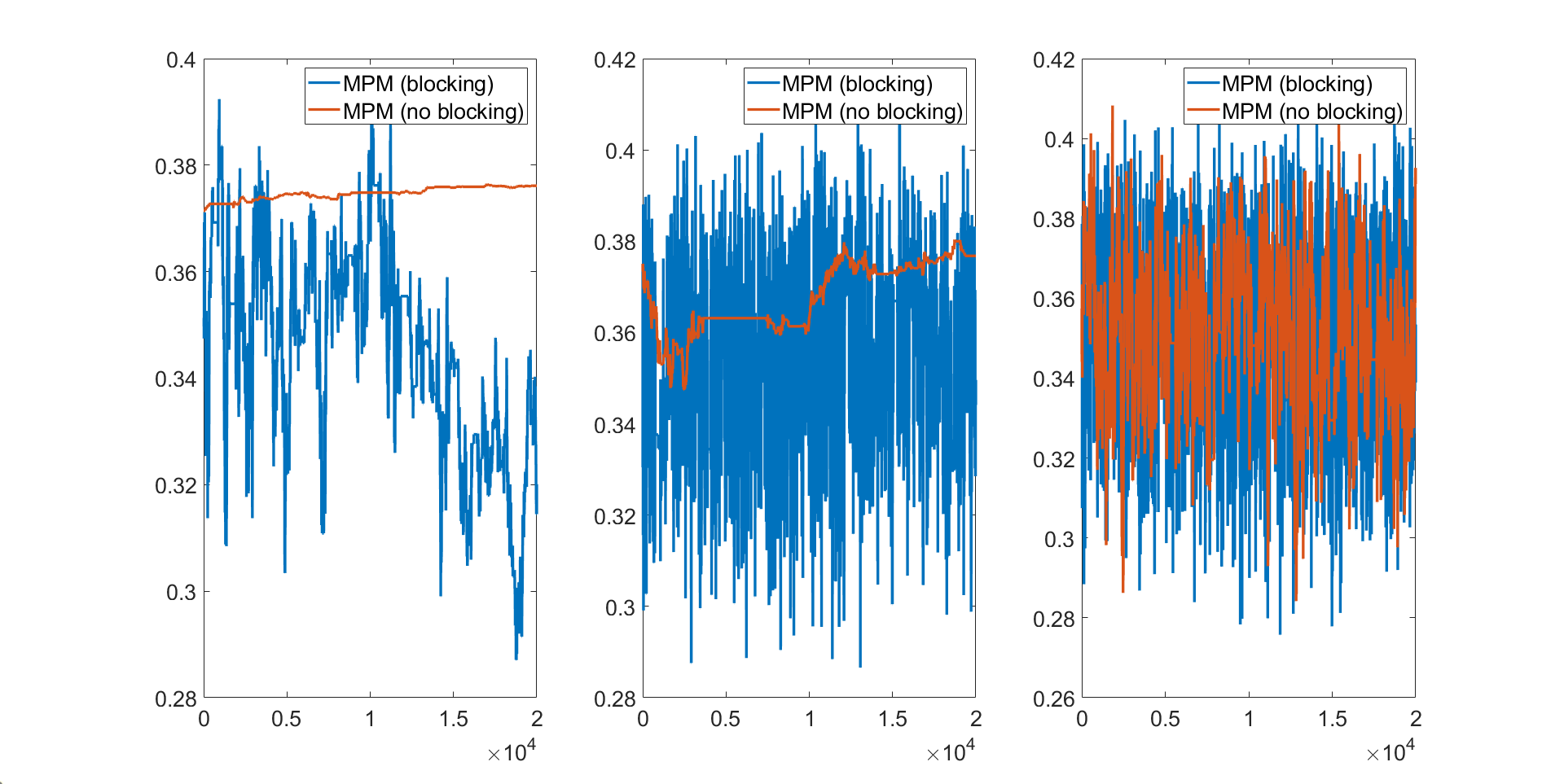
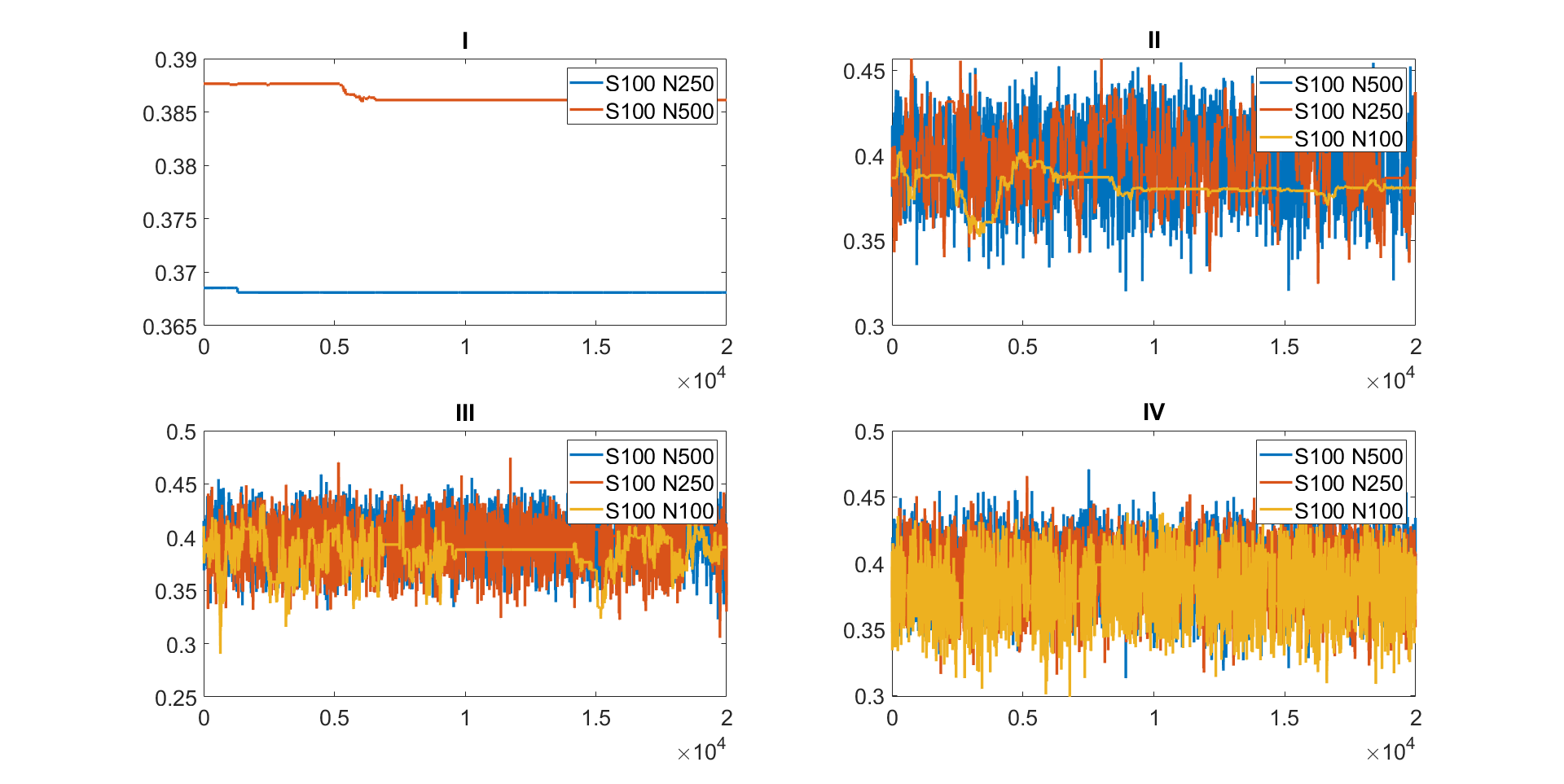
Figure 2 shows the trace plots of the parameter $\theta$ estimated using the MPM algorithm with the different trimmed means for estimating the 10 dimensional linear Gaussian state space model with $T=200$. The figure shows that: (1) the MCMC chain gets stuck for the 5% trimmed mean approach with $S=100$ and $N=250$ and $N=500$ and for the 10% trimmed mean approach with $S=100$ and $N=100$; (2) the 10% trimmed mean approach requires at least $S=100$ and $N=250$ to make the MCMC chain mix well; (3) the 25% trimmed mean approach is the most efficient sampler as its MCMC chain does not get stuck even with $S=100$ and $N=100$. Figure 1 compares the MPM algorithms with and without blocking with $S=100$ and $N=250$ for estimating the 10 dimensional linear Gaussian state space model with $T=300$. The figure shows that the MPM (no blocking) with 5% and 10% trimmed means get stuck and the MPM (no blocking) with 25% trimmed means mixes poorly. The $\widehat{\textrm{IF}}$ of the MPM (blocking) with 25% trimmed mean is $9.624$ times smaller than the MPM (no blocking) with 25% trimmed mean. All three panels show that the MPM (blocking) algorithms using trimmed means perform better than the MPM (no blocking). This suggests the usefulness of the MPM (blocking) sampling scheme.

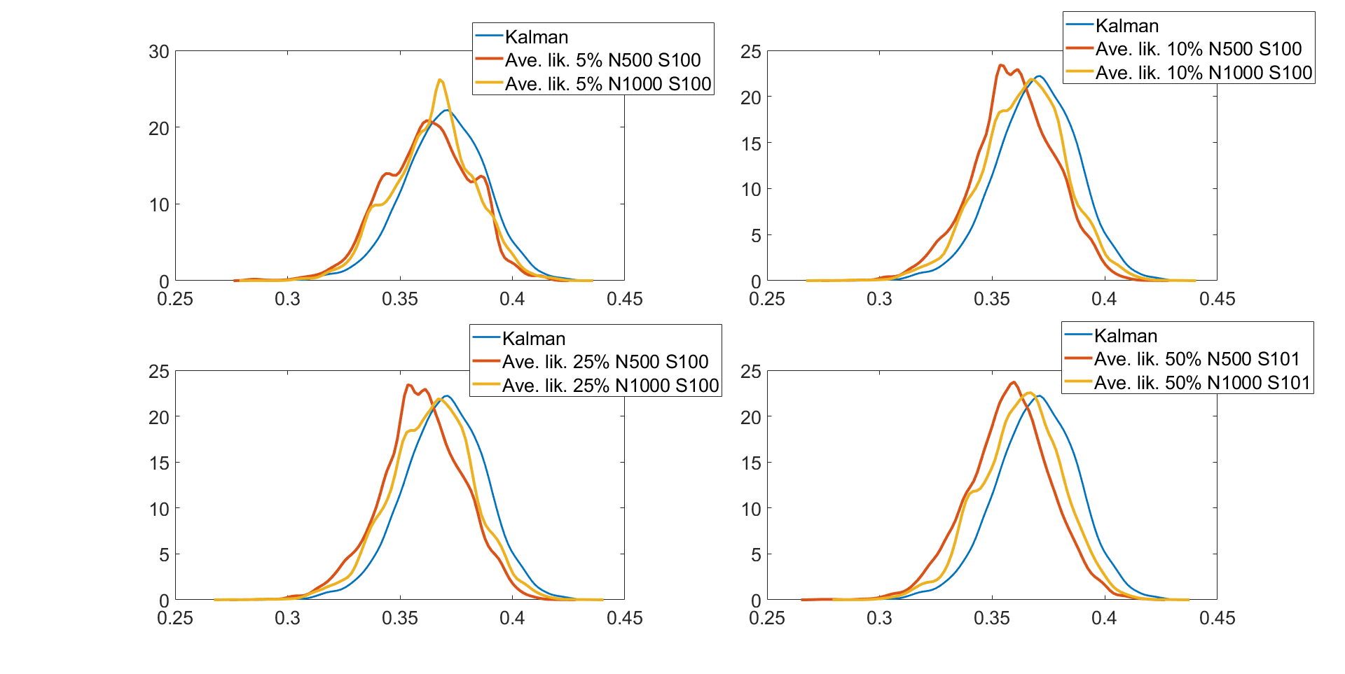
Table 3 shows the $\widehat{\textrm{IF}}$, $\widehat{\textrm{TNIF}}$, and $\widehat{\textrm{RTNIF}}$ values for the parameter $\theta$ in the linear Gaussian state space model with $d=10$ dimensions and $T=300$ time periods estimated using the following five different MCMC samplers: (1) the correlated PMMH of Deligiannidis et al., (2018), (2) the MPM with 5% trimmed mean, (3) the MPM with 10% trimmed mean, (4) the MPM with 25% trimmed mean, and (5) the MPM with 50% trimmed mean. In this paper, instead of using the Hilbert sorting method, we implement the correlated PMMH using the fast multidimensional Euclidean sorting method in section 2.4. The computing time reported in the table is the time to run a single particle filter for the CPM and $S$ particle filters for the MPM approach. The table shows the following points. (1) The correlated PMMH requires more than $50000$ particles to improve the mixing of the MCMC chain for the parameter $\theta$. (2) The CPU time for running a single particle filter with $N=50000$ particles is $4.09$ times higher than running multiple particle filters with $S=100$ and $N=500$. The MPM method can be much faster than the CPM method if it is run using high-performance computing with a large number of cores. (3) The MPM allows us to use much smaller number of particles for each independent PF and these multiple PFs can be run independently. (4) The $\widehat{\textrm{IF}}$ values for the parameter $\theta$ estimated using the correlated PMMH with $N=50000$ particles is $11.05$, $41.93$, $46.12$, and $56.37$ times larger than the 5%, 10%, 25%, and 50% trimmed means approaches with $S=100$ and $N=500$ particles, respectively. (5) In terms of $\widehat{\textrm{RTNIF}}$, the 5%, 10%, 25%, and 50% trimmed means with $S=100$ and $N=500$ are $45.27$, $171.52$, $188.67$, and $230.60$ times smaller than the correlated PMMH with $N=50000$ particles. (6) The best sampler for this example is the 50% trimmed mean approach with $S=100$ and $N=250$ particles. Table LABEL:tabledim10T200 in section S4 of the online supplement gives similar results for the 10 dimensional linear Gaussian state space model with $T=200$. Figure 3 shows the kernel density estimates of the parameter $\theta$ estimated using Metropolis-Hastings algorithm with the (exact) Kalman filter method and the MPM algorithm with 5%, 10%, 25%, and 50% trimmed means of the likelihood. The figure shows the approximate posteriors obtained by various approaches using trimmed means are very close to the true posterior. Similar results are obtained for the case $d=10$ dimensions and $T=200$ time periods given in Figure S1 in Section S4 of the online supplement. Figure S1 also shows that the approximate posterior obtained using the MPM with trimmed mean of the likelihood is very close to the exact posterior obtained using the correlated PMMH.

In summary, the example suggests that: (1) for a high dimensional state space model, there is no substantial reduction in the variance of the log of the estimated likelihood for the method which uses the average of the likelihood from $S$ particle filters when $S$ and/or $N$ increases. Methods that use trimmed means of the likelihood reduce the variance substantially when $S$ and/or $N$ increases; (2) the 25% and 50% trimmed means approaches give the smallest variance of the log of the estimated likelihood for all cases; (3) the MPM method with 50% trimmed mean is best at maintaining the correlation between the logs of the estimated likelihoods in successive iterates; (4) the MPM (blocking) method is more efficient than the MPM (no blocking) for the same values of $S$ and $N$; (5) the approximate approaches that use the trimmed means of the likelihood gives accurate approximations to the true posterior; (6) the best sampler for estimating the 10 dimensional linear Gaussian state space model with $T=300$ is the 50% trimmed mean approach with $S=100$ and $N=250$ particles; (7) the MPM allows us to use much smaller number of particles for each independent PF and these multiple PFs can be run independently. These approaches can be made much faster if they are run using a high-performance computer cluster with a large number of cores.

Table 3: Comparing the performance of different PMMH samplers with different number of particle filters $S$ and different number of particles $N$ in each particle filter for estimating the linear Gaussian state space model using a simulate dataset with $T=300$ and $d=10$ dimensions. Sampler I: Correlated PMMH of Deligiannidis et al., (2018). Sampler II: MPM with 5% trimmed mean. Sampler III: MPM with 10% trimmed mean. Sampler IV: MPM with 25% trimmed mean. Sampler V: MPM with 50% trimmed mean. Time denotes the time taken in seconds for one iteration of the method. The $\widehat{\textrm{IF}}$, CT, and $\widehat{\textrm{RTNIF}}$ entries in columns headed I to V are relative to the entries in column V (MPM with 50% trimmed mean with $N=250$ and $S=100$). The entries in column ”V actual” are the actual $\widehat{\textrm{IF}}$, CT, and $\widehat{\textrm{RTNIF}}$ values for estimator V. For example, the entry on row 5, column I is 415.08, which means the $\widehat{\textrm{RTNIF}}$ is 415.08 times the corresponding $\widehat{\textrm{RTNIF}}$ in column V (MPM with 50% trimmed mean with $N=250$ and $S=100$).

.

	I	II		III		IV		V		V actual
N	50000	250	500	250	500	250	500	250	500	250	500
S	1	100	100	100	100	100	100	100	100	100	100
$\widehat{\textrm{IF}}$	50.73	88.09	4.59	3.03	1.21	1.40	1.10	1.00	0.90	9.98	9.00
CT	8.18	1.00	2.00	1.00	2.00	1.00	2.00	1.00	2.00	0.99	1.98
$\widehat{\textrm{RTNIF}}$	415.08	88.10	9.17	3.03	2.42	1.40	2.20	1.00	1.80	9.88	17.82

Figure 1: Left: Trace plots of the parameter $\theta$ estimated using (1) MPM (blocking) with 5% trimmed mean and (2) MPM (no blocking) with 5% trimmed mean. Middle: Trace plots of the parameter $\theta$ estimated using (1) MPM (blocking) with 10% trimmed mean and (2) MPM (no blocking) with 10% trimmed mean. Right: Trace plots of the parameter $\theta$ estimated using (1) MPM (blocking) with 25% trimmed mean and (2) MPM (no blocking) with 25% trimmed mean. Linear Gaussian space model with $d=10$ dimensions, $T=300$ time periods, the number of particle filters $S=100$, and the number of particles in each particle filter $N=250$.

Figure 2: Trace plots of the parameter $\theta$ of the linear Gaussian state space model with $d=10$ dimensions and $T=200$ time periods estimated using different MPM samplers with different number of particle filters $S$ and number of particles $N$ in each particle filter: (I) MPM with mean likelihood estimate, (II) MPM with 5% trimmed mean estimate, (III) MPM with 10% trimmed mean estimate, (IV) MPM with 25% trimmed mean estimate.

Figure 3: Linear Gaussian state space model with $d=10,T=300$. Kernel density estimates of the posterior density of $\theta$ estimated using: Top Left: (1) Metropolis-Hastings with exact likelihood; (2) MPM with 5% trimmed mean estimate, $S=100,N=500$; (3) MPM with 5% trimmed mean, $S=100,N=1000$. Top Right: (1) Metropolis-Hastings with exact likelihood; (2) MPM with the 10% trimmed mean estimate, $S=100,N=500$; (3) MPM with 10% trimmed mean estimate, $S=100$, $N=1000$. Bottom Left: (1) Metropolis-Hastings using the exact likelihood; (2) MPM with 25% trimmed mean estimate of the likelihood, $S=100$, $N=500$; (3) MPM with 25% trimmed mean estimate of the likelihood, $S=100$, $N=1000$. Bottom Right: (1) Metropolis-Hastings algorithm with exact likelihood; (2) MPM with 50% trimmed mean estimate of the likelihood, $S=101$, $N=500$; (3) MPM with 50% trimmed mean estimate of the likelihood, $S=101$, $N=1000$.

3.3 Multivariate Stochastic Volatility in Mean Model

This section investigates the performance of the proposed MPM samplers for estimating large multivariate stochastic volatility in mean models (see, e.g., Carriero et al., , 2018; Cross et al., , 2021), where each of the log volatility processes follows a GARCH (Generalized Autoregressive Conditional Heteroskedasticity) diffusion process (Shephard et al., , 2004). The GARCH diffusion model does not have a closed form state transition density, making it challenging to estimate using the Gibbs type MCMC sampler used in Cross et al., (2021). It is well-known that the Gibbs sampler is inefficient for generating parameters for a diffusion process, especially for the variance parameter $\tau^{2}$ (Stramer and Bognar, , 2011). Conversely, MPM samplers can efficiently estimate models with non-closed form state transition densities, making them well-suited for the GARCH diffusion model. This section demonstrates that MPM samplers can estimate this model efficiently and overcome the limitations of the Gibbs sampler.

Suppose that $P_{t}$ is a $d\times 1$ vector of daily stock prices and define $y_{t}=\log P_{t}-\log P_{t-1}$ as the log-return of the stocks. Let $h_{i,t}$ be the log-volatility process of the $i$th stock at time $t$. We also define, $h_{\cdotp,t}=\left(h_{1,t},...,h_{d,t}\right)^{\top}$ and $h_{i,\cdotp}=\left(h_{i,1},...,h_{i,T}\right)^{\top}$. The model for $y_{t}$ is

$$y_{t}=Ah_{\cdot,t}+\epsilon_{t},\;\epsilon_{t}\sim N\left(0,\Sigma_{t}\right),$$ (8)

where $A$ is a $d\times d$ matrix that captures the effects of log-volatilities on the levels of the variables. The time-varying error covariance matrix $\Sigma_{t}$ depends on the unobserved latent variables $h_{\cdotp,t}$ such that

$$\Sigma_{t}:=\textrm{diag}\left(\exp\left(h_{1,t}\right),...,\exp\left(h_{d,t}\right)\right).$$ (9)

Each log-volatility $h_{i,t}$ is assumed to follow a continuous time GARCH diffusion process (Shephard et al., , 2004) satisfying

$$dh_{i,t}=\left\{\alpha\left(\mu-\exp\left(h_{i,t}\right)\right)\exp\left(-h_{i,t}\right)-\frac{\tau^{2}}{2}\right\}dt+\tau dW_{i,t},$$ (10)

for $i=1,...,d$, where the $W_{i,t}$ are independent Wiener processes. The following Euler scheme approximates the evolution of the log-volatilities ${h}_{i,t}$ in (10) by placing $M-1$ evenly spaced points between times $t$ and $t+1$. We denote the intermediate volatility components by $h_{i,t,1},...,h_{i,t,M-1}$, and it is convenient to set $h_{i,t,0}=h_{i,t}$ and $h_{i,t,M}=h_{i,t+1}$. The equation for the Euler evolution, starting at $h_{i,t,0}$ is (see, for example, Stramer and Bognar, (2011), pg. 234)

$$h_{i,t,j+1}|h_{i,t,j}\sim N\left(h_{i,t,j}+\left\{\alpha\left(\mu-\exp\left(h_{i,t,j}\right)\right)\exp\left(-h_{i,t,j}\right)-\frac{\tau^{2}}{2}\right\}\delta,\tau^{2}\delta\right),$$ (11)

for $j=0,...,M-1$, where $\delta=1/M$. The initial state of $h_{i,t}$ is assumed normally distributed $N(0,1)$ for $i=1,...,d$. For this example, we assume for simplicity that the parameters $\mu$, $\alpha$, and $\tau^{2}$ are the same across all stocks and $A^{i,j}=\psi^{|i-j|+1}$ for $i<j$. This gives the same number of parameters regardless of the dimension of the stock returns so that we can focus on comparing different PMMH samplers.

We first report on a simulation study for the above model. We simulated ten independent datasets from the model described above with $d=20$ dimensions and $T=100$ observations. The true parameters are $\alpha=2$, $\mu=1.81$, $\tau^{2}=0.38$, and $\psi=0.01$. The priors are $\alpha\sim G\left(1,1\right)$, $\tau^{2}\sim G\left(0.5,0.5\right)$, $\mu\sim G\left(1,1\right)$, and $\psi\sim N\left(0,1\right)$. These prior densities are non-informative and cover almost all possible values in practice. We use $M=3$ latent points for the Euler approximations of the state transition densities. For each dataset, we run the MPM sampler with the 25% trimmed mean approach for $25000$ iterations; the initial $5000$ iterations are discarded as warm up. The particle filter and the parameter samplers are implemented in Matlab running on 20 CPU cores, a high performance computer cluster. The adaptive random walk proposal of Roberts and Rosenthal, (2009) is used for all samplers.

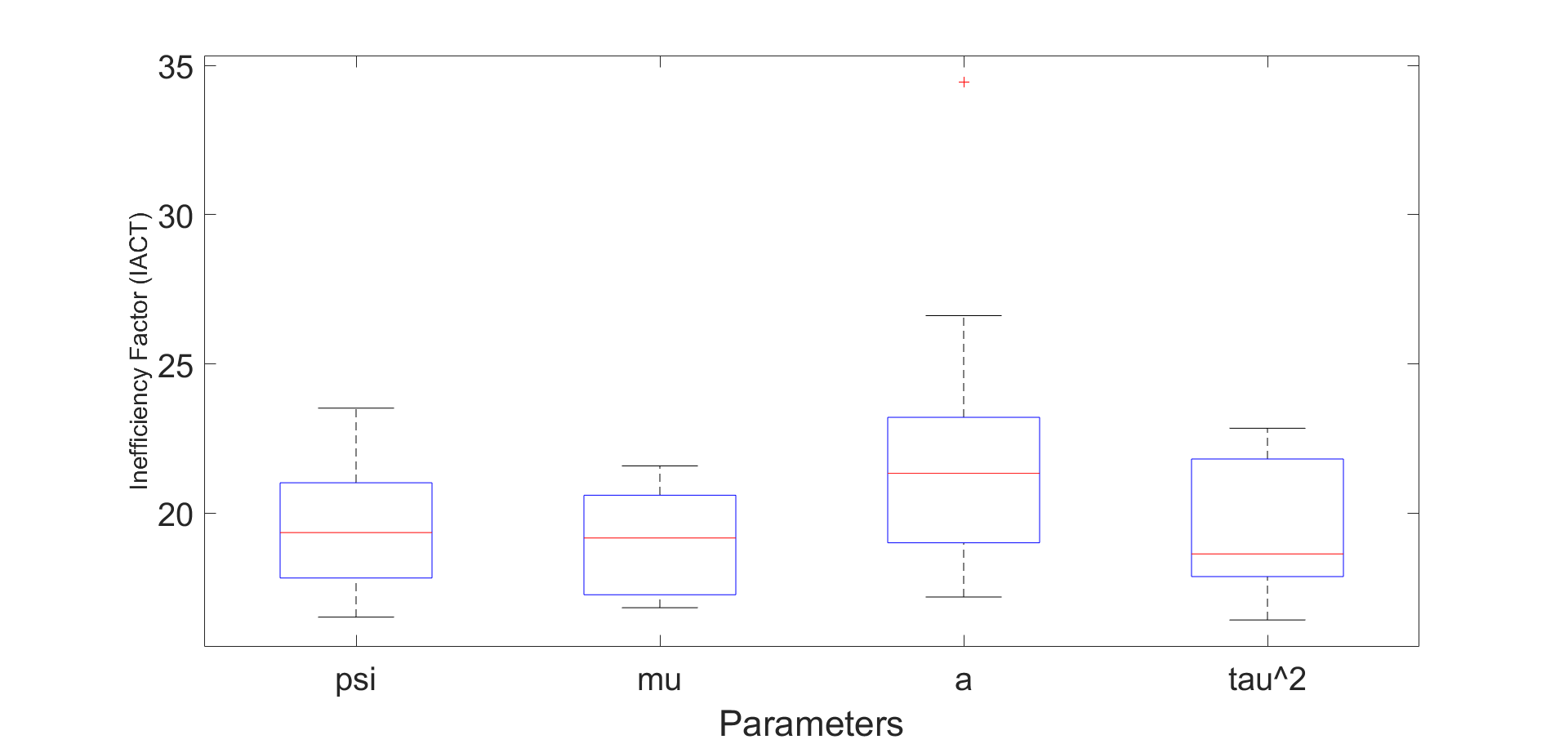
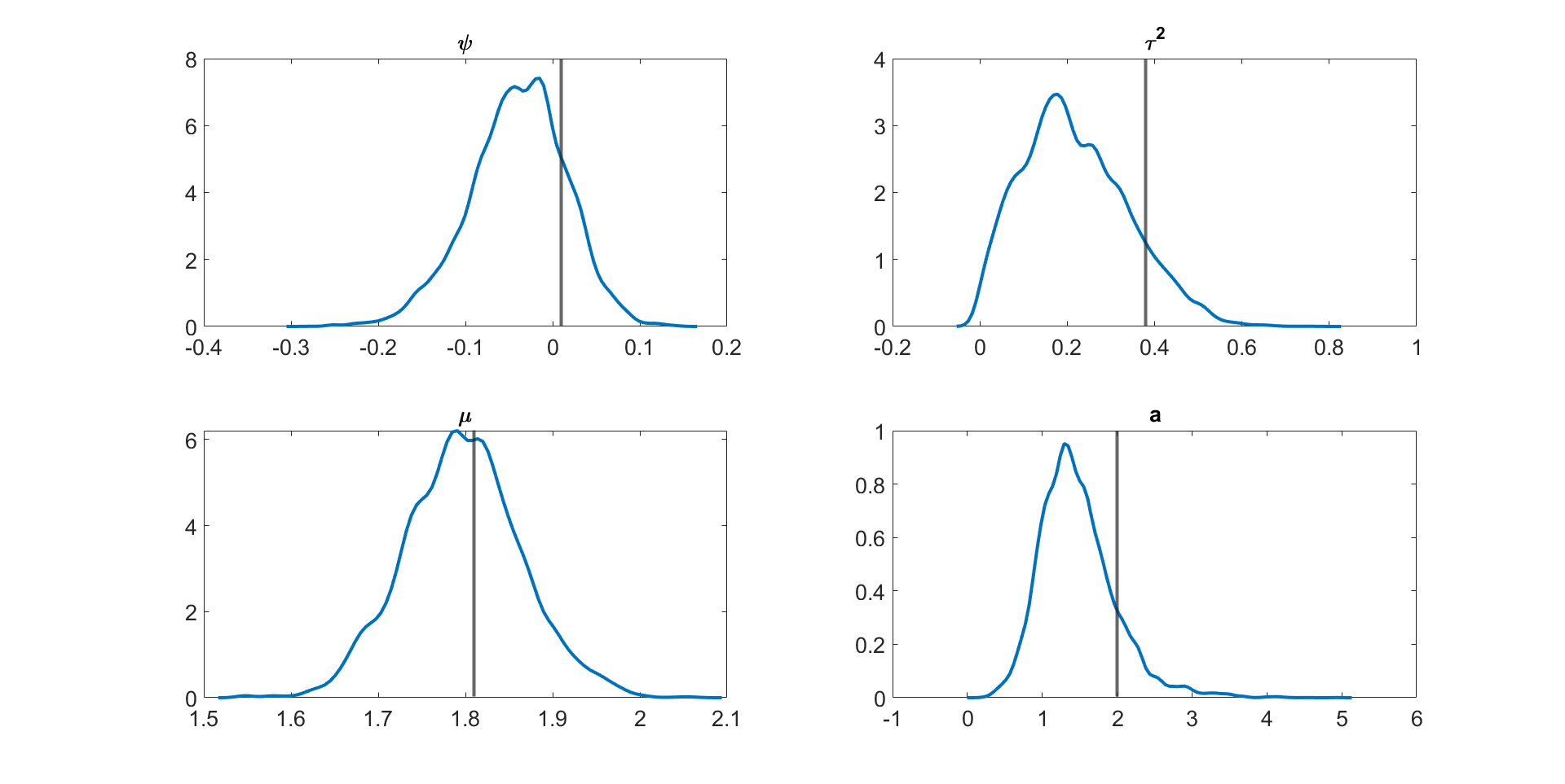
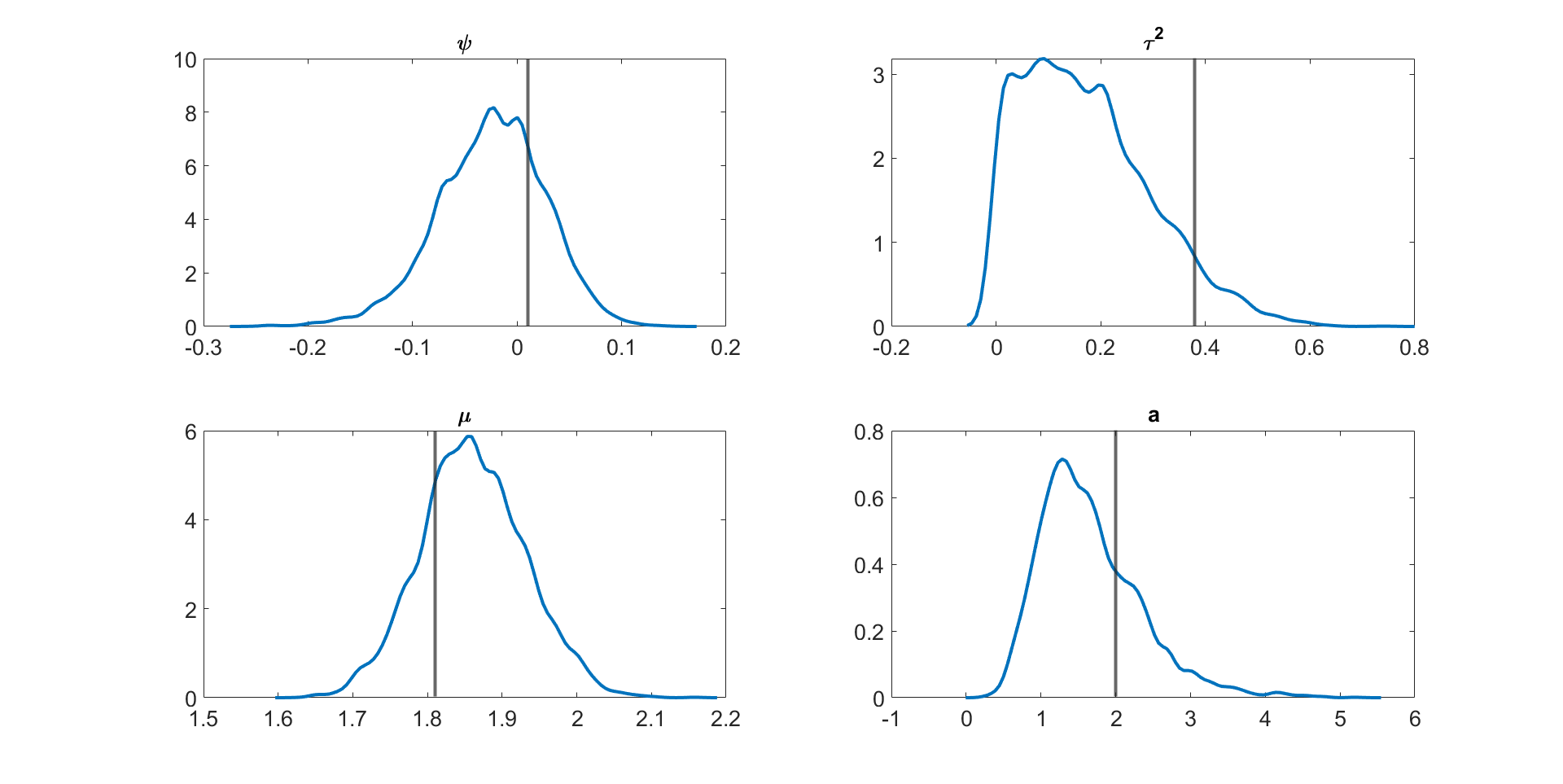
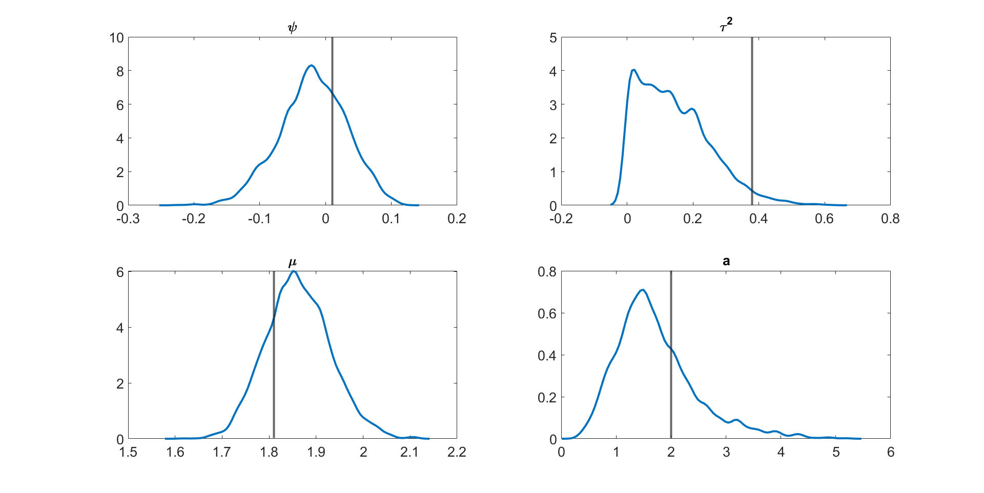
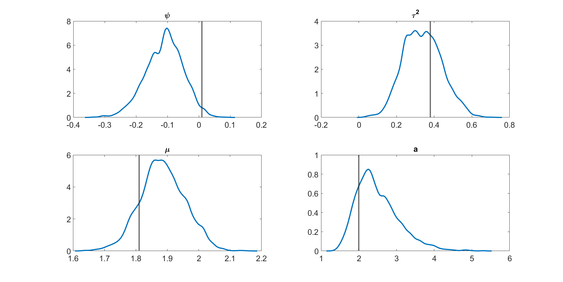
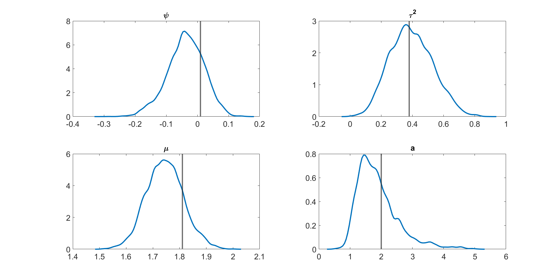
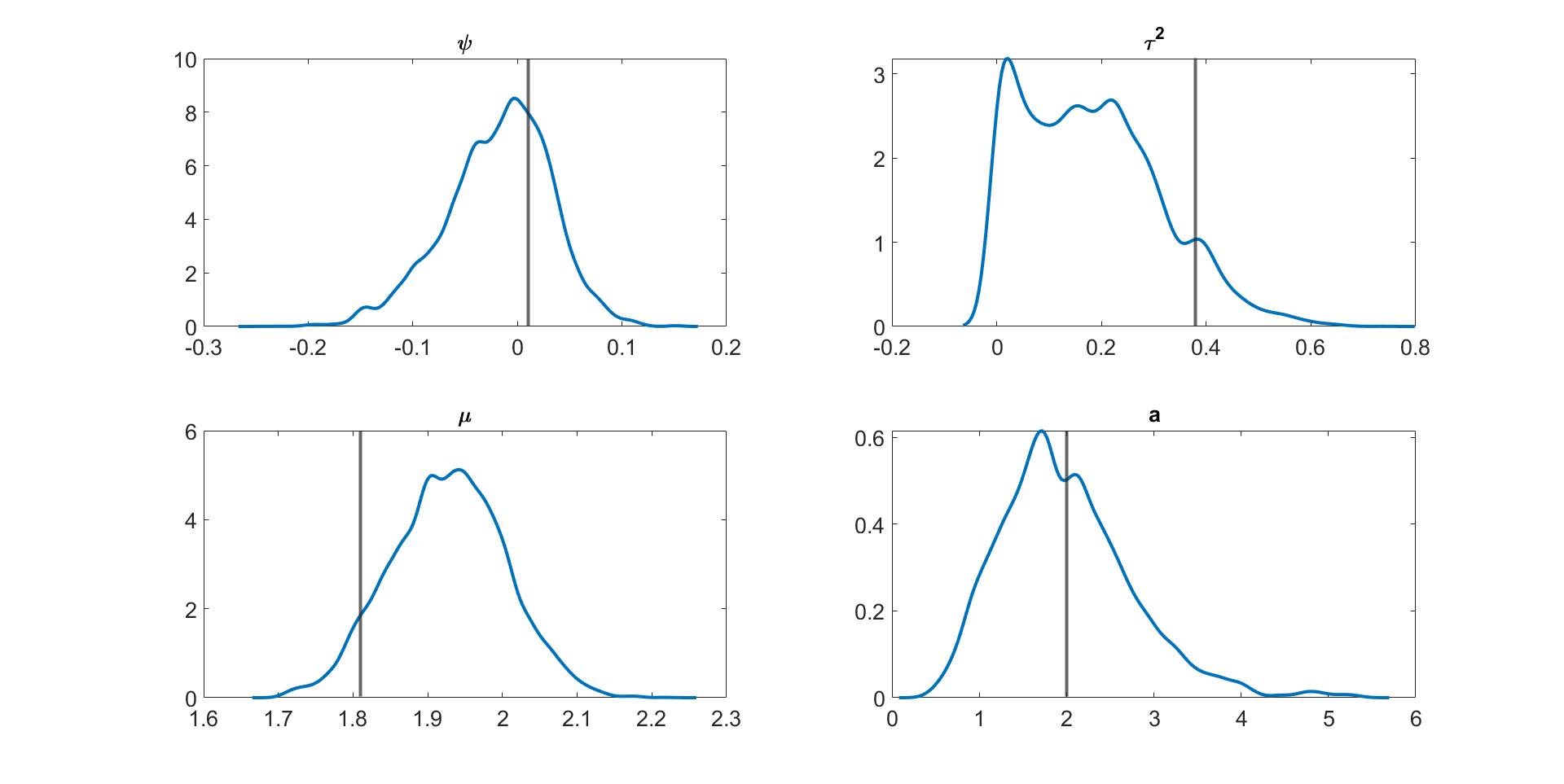
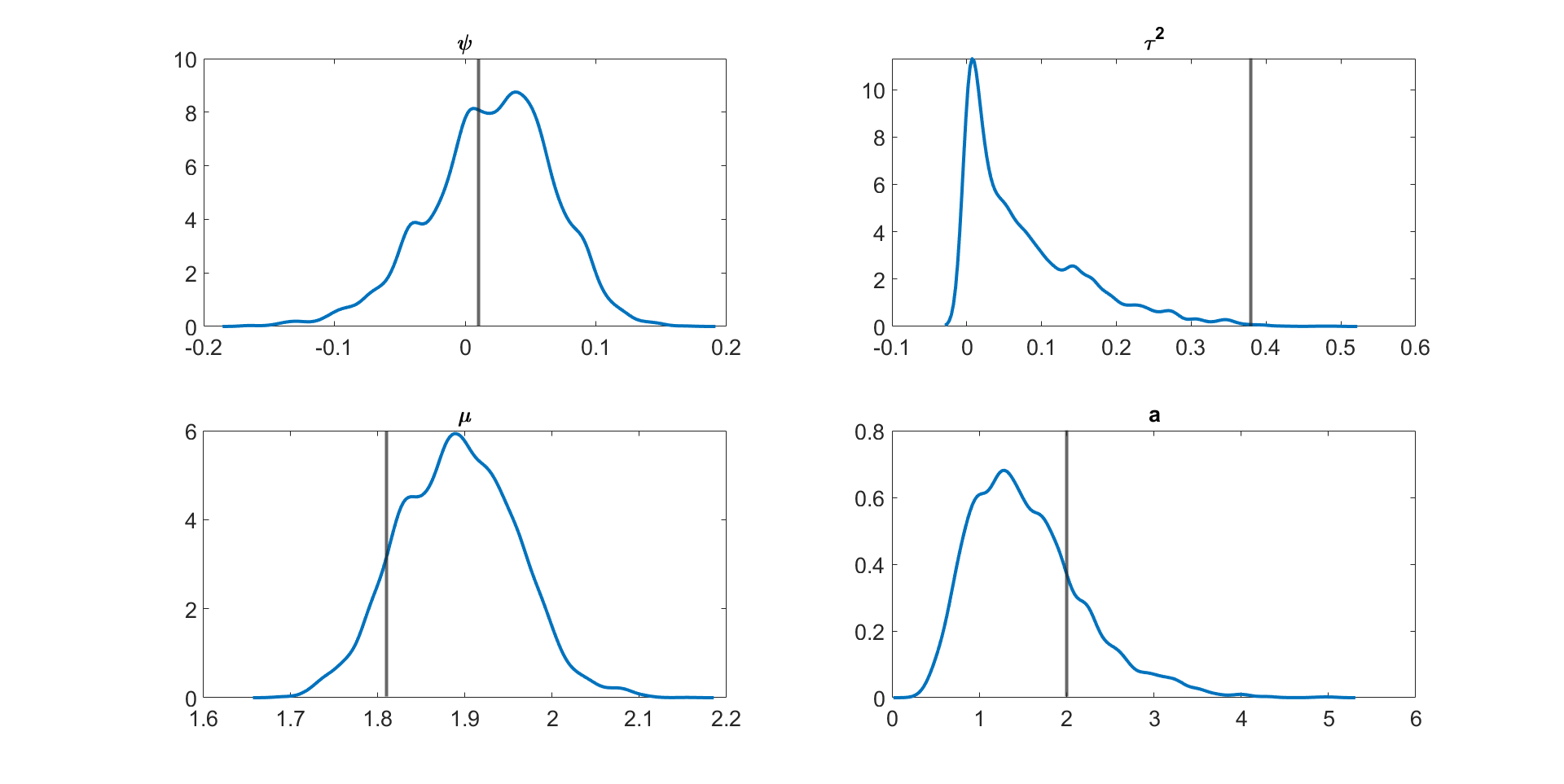
Figure 4 and Figures S3 to S11 in section S5 of the online supplement show the kernel density estimates of the parameters of the multivariate stochastic volatility in mean model described above estimated by the MPM sampler ($S=100$ and $N=250$) using a 25% trimmed mean; the vertical lines show the true parameter values. The figures show that the model parameters are accurately estimated. Figure 5 shows the inefficiency factors ($\widehat{\textrm{IF}}$) of the parameters over 10 simulated datasets with $d=20$ dimensions and $T=100$ time periods. The results suggest that the MPM sampler with only $N=250$ particles and $S=100$ particle filters is efficient because the $\widehat{\textrm{IF}}$ values of the parameters are reasonably small.

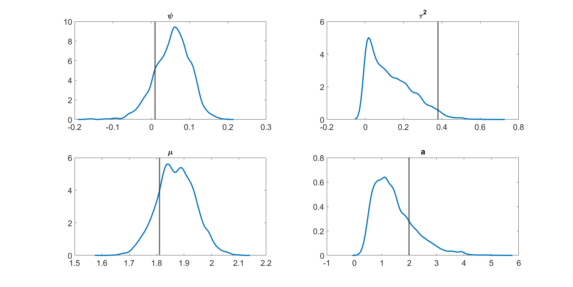
Figure 4: Kernel density estimates of the parameters of the multivariate stochastic volatility in mean model estimated using MPM with a 25% trimmed mean estimate of the likelihood based on a simulated dataset (data 1) with $d=20$ and $T=100$.

Figure 5: The inefficiency factors ($\widehat{\textrm{IF}}$) of the parameters of the multivariate stochastic volatility in mean model estimated using MPM with a 25% trimmed mean estimate of the likelihood for 10 simulated datasets with $d=20$ and $T=100$.

We now apply the methods to a sample of daily US industry stock returns data obtained from the Kenneth French website, using a sample from January 4th, 2021 to the 26th of May, 2021, a total of 100 observations.

Table 4 shows the $\widehat{\textrm{IF}}$, $\widehat{\textrm{TNIF}}$, and $\widehat{\textrm{RTNIF}}$ for the parameters of the 20 dimensional multivariate stochastic volatility in mean model estimated using (1) the correlated PMMH, (2) the MPM sampler with the 25% trimmed mean of the likelihood estimate, and (3) the MPM sampler with the 50% trimmed mean of the likelihood estimate. The table shows that: (1) the MCMC chain obtained using the correlated PMMH with $N=100000$ still gets stuck; (2) the CPU time for the correlated PMMH with $N=100000$ particles is $26$ times slower than the MPM algorithm with $S=250$ and $N=100$; (3) the MPM sampler with $N=250$ and $S=100$ is less efficient than the MPM sampler with $N=100$ and $S=250$. The MPM sampler with $N=100$ and $S=250$ can be made more efficient by running it on a high-performance computer cluster with many cores; (4) the best sampler in terms of $\widehat{\textrm{TNIF}}_{\textrm{MEAN}}$ and $\widehat{\textrm{TNIF}}_{\textrm{MAX}}$ for estimating the 20 dimensional multivariate stochastic volatility in mean model is the MPM sampler with a 50% trimmed mean with $S=250$ and $N=100$.

Table 5 shows the $\widehat{\textrm{IF}}$, $\widehat{\textrm{TNIF}}$, and $\widehat{\textrm{RTNIF}}$ for the parameters of the $d=30$ dimensional multivariate stochastic volatility in the mean model estimated using: (1) the MPM sampler with the 25% trimmed mean of the likelihood, and (2) the MPM sampler with 50% trimmed mean of the likelihood. We do not consider the correlated PMMH as it is very expensive to run for this high dimensional model. The table shows that (1) increasing the number of particle filters from $S=100$ to $S=200$ reduces the $\widehat{\textrm{IF}}$, but increases the computational time substantially. However, the computational time can be reduced by using a high performance computer cluster with a larger number of cores; (2) the MPM sampler with $N=500$ and $S=100$ is less efficient than the MPM sampler with $N=250$ and $S=200$. We recommend that if there is access to large computing resources, then the number of particle filters $S$ should be increased while keeping the number of particles $N$ in each particle filter reasonably small.

Table 4: Comparing the performance of different PMMH samplers with different numbers $S$ of particle filters and different number $N$ of particles in each particle filter for estimating a multivariate stochastic volatility in mean model with GARCH diffusion processes using a real dataset with $T=100$ and $d=20$. The model parameters are $\psi$, $\mu$, $a$, and $\tau^{2}$. Sampler I: Correlated PMMH of Deligiannidis et al., (2018). Sampler II: MPM with 25% trimmed mean. Sampler III: MPM with 50% trimmed mean. Time denotes the time taken in seconds for one iteration of the method. The RTNIF is the TNIF relative to the MPM with 25% trimmed mean with $S=100$ and $N=250$.

Param.	I	II		III
N	100000	250	100	250	100
S	1	100	250	100	250
$\psi$	NA	$97.621$	$67.459$	$83.523$	$62.680$
$\mu$	NA	$65.678$	$42.299$	$52.293$	$39.390$
$a$	NA	$20.037$	$10.409$	$12.857$	$9.490$
$\tau^{2}$	NA	$56.617$	$32.900$	$43.705$	$37.928$
$\widehat{\textrm{IF}_{\psi,\textrm{MAX}}}$	NA	$97.621$	$67.459$	$83.523$	$62.680$
$\widehat{\textrm{TNIF}}_{\textrm{MAX}}$	NA	$173.765$	$124.799$	$148.671$	$115.958$
$\widehat{\textrm{RTNIF}}_{\textrm{MAX}}$	NA	$1$	$0.718$	$0.856$	$0.667$
$\widehat{\textrm{IF}_{\psi,\textrm{MEAN}}}$	NA	$59.988$	$38.267$	$48.095$	$37.372$
$\widehat{\textrm{TNIF}}_{\textrm{MEAN}}$	NA	$106.779$	$70.794$	$85.609$	$69.138$
$\widehat{\textrm{RTNIF}}_{\textrm{MEAN}}$	NA	$1$	$0.663$	$0.802$	$0.647$
Time	47.65	1.78	1.85	1.78	1.85

Table 5: Comparing the performance of different PMMH samplers with different number of particle filters S and different number of particles N in each particle filter for estimating multivariate stochastic volatility in mean model with GARCH diffusion processes using a real dataset with $T=100$ and $d=30$. The model parameters are $\psi$, $\mu$, $a$, and $\tau^{2}$. Sampler I: MPM with 25% trimmed mean. Sampler II: MPM with 50% trimmed mean. Time is the time in seconds for one iteration of the method. The RTNIF is the TNIF relative to the MPM with 25% trimmed mean with $S=100$ and $N=250$.

Param.	I			II
N	250	250	500	250	250
S	100	200	100	100	200
$\psi$	$183.559$	$124.258$	$227.685$	$151.745$	$80.073$
$\mu$	$74.070$	$49.250$	$384.767$	$74.485$	$45.554$
$a$	$46.159$	$45.662$	$126.968$	$32.721$	$14.753$
$\tau^{2}$	$102.234$	$70.255$	$218.866$	$78.171$	$42.075$
$\widehat{\textrm{IF}_{\psi,\textrm{MAX}}}$	$183.559$	$124.258$	$384.767$	$151.745$	$80.073$
$\widehat{\textrm{TNIF}}_{\textrm{MAX}}$	$523.143$	$877.262$	$3351.321$	$432.473$	$565.315$
$\widehat{\textrm{RTNIF}}_{\textrm{MAX}}$	$1$	$1.677$	$6.406$	$0.827$	$1.081$
$\widehat{\textrm{IF}_{\psi,\textrm{MEAN}}}$	$101.505$	$72.356$	$239.571$	$84.280$	$45.614$
$\widehat{\textrm{TNIF}}_{\textrm{MEAN}}$	$289.289$	$510.833$	$2077.953$	$240.198$	$322.035$
$\widehat{\textrm{RTNIF}}_{\textrm{MEAN}}$	$1$	$1.766$	$7.183$	$0.830$	$1.113$
Time	2.85	7.06	8.71	2.85	7.06

3.4 DSGE models

In this section, we evaluate the effectiveness of the MPM samplers for estimating two non-linear DSGE models: the small scale and medium scale DSGE models as detailed in sections S8 and S9 of the online supplement. Due to the large dimension of the states compared to the dimension of the disturbances in these state space models, we employ the disturbance filter method introduced in section 2.5.

The state transition densities of the two non-linear DSGE models are intractable. Section S3 of the online supplement describes the state space representation of these models, which are solved using Dynare.

3.4.1 Nonlinear Small Scale DSGE Model

This section reports on how well a number of PMMH samplers of interest estimate the parameters of the nonlinear (second order) small scale DSGE model. The small scale DSGE model follows the setting in Herbst and Schorfheide, (2019) with nominal rigidities through price adjustment costs following Rotemberg, (1982), and three structural shocks. There are $4$ state variables, $4$ control variables ($8$ variables combining the state and control variables) and $3$ exogenous shocks in the model. We estimate this model using $3$ observables, which means that the dimensions of $y_{t}$, the state vector and the disturbance vector are $3$, $8$, and $3$, respectively. Section S8 of the online supplement describes the model.

In this section, we use the delayed acceptance version of the MPM algorithm, calling it “delayed acceptance multiple PMMH” (DA-MPM), to speed up the computation. The delayed acceptance sampler (Christen and Fox, , 2005) avoids computing the expensive likelihood estimate if it is likely that the proposed draw will ultimately be rejected. The first accept-reject stage uses a cheap (or deterministic) approximation to the likelihood instead of the expensive likelihood estimate in the MH acceptance ratio. The particle filter is then used to estimate the likelihood only for a proposal that is accepted in the first stage; a second accept-reject stage ensures that detailed balance is satisfied with respect to the true posterior. We use the likelihood obtained from the central difference Kalman filter (CDKF) proposed by Norgaard et al., (2000) in the first accept-reject stage of the delayed acceptance scheme. Section  S2 of the online supplement gives further details. The dimension of states is usually much larger than the dimension of the disturbances for the DSGE models. Two different sorting methods are also considered. The first sorts the state particles and the second sorts the disturbance particles using the sorting algorithm in section 2.4.

The PMMH samplers considered are: (1) The MPM (0% trimmed mean) with the auxiliary disturbance particle filter (ADPF), disturbance sorting, and the correlation between random numbers used in estimating the log of estimated likelihoods set to $\rho_{u}=0.9$; (2) the MPM (10% trimmed mean) with the ADPF, disturbance sorting, and the $\rho_{u}=0.9$; (3) the MPM (25% trimmed mean) with the ADPF, disturbance sorting, and the $\rho_{u}=0.9$; (4) the MPM (25% trimmed mean) with the ADPF, disturbance sorting, and $\rho_{u}=0$, (5) the MPM (25% trimmed mean) with the ADPF, state sorting, and $\rho_{u}=0.9$; (6) the delayed acceptance MPM (DA-MPM) (25% trimmed mean) with ADPF, disturbance sorting, and the $\rho_{u}=0.9$; (7) the MPM (50% trimmed mean) with the ADPF, disturbance sorting, and the $\rho_{u}=0.9$; (8) the MPM (0% trimmed mean) with the bootstrap particle filter, disturbance sorting, and the $\rho_{u}=0.9$; (9) the correlated PMMH with $\rho_{u}=0.9$, the bootstrap particle filter, and disturbance sorting. Each sampler ran for $25000$ iterations, with the initial $5000$ iterations discarded as burn-in. We use the adaptive random walk proposal of Roberts and Rosenthal, (2009) for $q\left(\theta^{{}^{\prime}}|\theta\right)$ and the adaptive scaling approach of Garthwaite et al., (2015) to tune the Metropolis-Hastings acceptance probability to $20\%$. Section S8 of the online supplement gives details on model specifications and model parameters. We include measurement error in the observation equation. The measurement error variances are estimated together with other parameters. All the samplers ran on a high performance computer cluster with 20 CPU cores. The real dataset is obtained from Herbst and Schorfheide, (2019), using data from 1983Q1 to 2013Q4, which includes the Great Recession with a total of $124$ observations for each series.

Table 6 reports the relative time normalised inefficiency factor ($\widehat{\textrm{RTNIF}}$) of a PMMH sampler relative to the DA-MPM (25% trimmed mean) with the ADPF, disturbance sorting, and $\rho_{u}=0.9$ for the non-linear small scale models with $T=124$ observations. The computing time reported in the table is the time to run a single particle filter for the CPM and $S$ particle filters for the MPM approach. The table shows that: (1) The MPM sampler (0% trimmed mean) with the ADPF, disturbance sorting, $\rho_{u}=0.9$, and $N=250$ particles is more efficient than the MPM sampler (0% trimmed mean) with the bootstrap particle filter, disturbance sorting, $\rho_{u}=0.9$, and $N=250$ particles with the MCMC chain obtained by the latter getting stuck. (2) The running time taken the MPM method with $S=100$ particles filters, each with $N=100$ particles and disturbance sorting is $9.73$ times faster than the CPM with $N=20000$ particles. (3) In terms of $\widehat{\textrm{RTNIF}}_{\textrm{MAX}}$, the performance of MPM samplers with 0%, 10%, 25%, and 50% trimmed means, ADPF, disturbance sorting, and $\rho_{u}=0.9$ are $3.15$, $90.77$, $103.04$, and $91.50$ times more efficient respectively, than the correlated PMMH with $N=20000$ particles. (4) In terms of $\widehat{\textrm{RTNIF}}_{\textrm{MAX}}$, the MPM (25% trimmed mean) with disturbance sorting, and $\rho_{u}=0.9$ is $1.38$ times more efficient than the MPM (25% trimmed mean) method with state sorting method and performs similarly to the MPM (25% trimmed mean) approach with ADPF, disturbance sorting, and $\rho_{u}=0$. (5) The delayed acceptance MPM (25% trimmed mean) is slightly more efficient than the MPM (25% trimmed mean) approach. The delayed acceptance algorithm is $5$ times faster on average because the target Metropolis-Hastings acceptance probability is set to $20\%$ using the Garthwaite et al., (2015) approach, but it has higher maximum $\widehat{\textrm{IF}}$ value. Table S8 in section S6 of the online supplement gives the details. (6) It is possible to use the tempered particle filter of Herbst and Schorfheide, (2019) within the MPM algorithm. However, the TPF is computationally expensive because of the tempering iterations and the random walk Metropolis-Hastings mutation steps. In summary, the best sampler with the smallest $\widehat{\textrm{RTNIF}}_{\textrm{MAX}}$ and $\widehat{\textrm{RTNIF}}_{\textrm{MEAN}}$ is the delayed acceptance MPM (DA-MPM) (25% trimmed mean) with ADPF, disturbance sorting, and $\rho_{u}=0.9$.

Table 6: Comparing the performance of different PMMH samplers with different number of particle filters $S$ and different number of particles $N$ in each particle filter for estimating small scale DSGE model using a real dataset with $T=124$ observations. Sampler I: MPM (0% trimmed mean, $\rho_{u}=0.9$, disturbance sorting, ADPF). Sampler II: MPM (10% trimmed mean, $\rho_{u}=0.9$, disturbance sorting, ADPF). Sampler III: MPM (25% trimmed mean, $\rho_{u}=0.9$, disturbance sorting, ADPF). Sampler IV: MPM (25% trimmed mean, $\rho_{u}=0$, disturbance sorting, ADPF). Sampler V: MPM (25% trimmed mean, $\rho_{u}=0.9$, state sorting, ADPF). Sampler VI: DA-MPM (25% trimmed mean, $\rho_{u}=0.9$, disturbance sorting, ADPF). Sampler VII: MPM (50% trimmed mean, $\rho_{u}=0.9$, disturbance sorting, ADPF). Sampler VIII: MPM (0% trimmed mean, $\rho_{u}=0.9$, disturbance sorting, bootstrap). Sampler IX: Correlated PMMH of Deligiannidis et al., (2018). Time denotes the time taken in seconds for one iteration of the method. The $\widehat{\textrm{IF}}_{\psi,\textrm{MAX}}$, $\widehat{\textrm{RTNIF}}_{\textrm{MAX}}$, $\widehat{\textrm{IF}}_{\psi,\textrm{MEAN}}$, and $\widehat{\textrm{RTNIF}}_{\textrm{MEAN}}$ entries in columns headed I to IX are relative to the entries in column VI. The entries in column ”VI actual” are the actual $\widehat{\textrm{IF}}_{\psi,\textrm{MAX}}$, $\widehat{\textrm{RTNIF}}_{\textrm{MAX}}$, $\widehat{\textrm{IF}}_{\psi,\textrm{MEAN}}$, and $\widehat{\textrm{RTNIF}}_{\textrm{MEAN}}$ for estimator VI. The numbers in bold are for the sampler with similar values of the $\widehat{\textrm{RTNIF}}_{\textrm{MAX}}$ and $\widehat{\textrm{RTNIF}}_{\textrm{MEAN}}$.

	I	II	III	IV	V	VI	VII	VIII	IX	VI actual
S	100	100	100	100	100	100	100	100	1	100
N	250	100	100	100	100	100	100	250	20000	100
$\widehat{\textrm{IF}}_{\psi,\textrm{MAX}}$	$3.73$	$0.25$	$0.22$	$0.25$	$0.28$	$1.00$	$0.39$	NA	$2.42$	$604.72$
$\widehat{\textrm{RTNIF}}_{\textrm{MAX}}$	$36.27$	1.26	1.11	1.25	$1.54$	1.00	$1.96$	NA	$114.37$	${66.52}$
$\widehat{\textrm{IF}}_{\psi,\textrm{MEAN}}$	$5.88$	$0.49$	$0.50$	$0.49$	$0.61$	$1.00$	$0.59$	NA	$3.32$	$190.74$
$\widehat{\textrm{TNIF}}_{\textrm{MEAN}}$	$57.23$	2.47	2.49	2.44	$3.41$	1.00	$2.93$	NA	$157.02$	${20.98}$
Time	9.73	5.00	5.00	5.00	5.55	1.00	$5.00$	6.82	47.27	0.11

3.4.2 Nonlinear Medium Scale DSGE Model

This section applies the MPM samplers with 50% trimmed mean for estimating the parameters of the second-order medium-scale DSGE model of Gust et al., (2017) discussed in Section S9 of the online supplement. The medium scale DSGE model is similar to the models in Christiano et al., (2005) and Smets and Wouters, (2007) with nominal rigidities in both wages and prices, habit formation in consumption, investment adjustment costs, along with five structural shocks. We do not consider the zero lower bound (ZLB) on the nominal interest rate because estimating such a model requires solving the fully nonlinear model using global methods instead of local perturbation techniques. The time taken to solve the fully nonlinear model depends on the choice of solution technique and can vary across methods such as value function iteration and time-iteration methods. Since the paper focuses on demonstrating the strength of the estimation algorithm, we restrict our sample to the period before the zero lower bound constraint on the nominal interest rate binds and the model can be solved (at a second order approximation) using perturbation methods. The estimation algorithm, however, can be applied to fully nonlinear models as well since the estimation step requires decision rules produced by the model solution (global or local methods).

The baseline model in Gust et al., (2017) consists of 12 state variables, 18 control variables (30 variables combining the state and control variables) and 5 exogenous shocks. We estimate this model using 5 observables; that means that the dimensions of $y_{t}$, the state vector and the disturbance vector are $5$, $30$, and $5$, respectively. We include measurement error in the observation equation and consider two cases. The measurement error variances are: (1) estimated and (2) fixed at the 25% of the sample variance of the observables over the estimation period. We use quarterly US data from 1983Q1 to 2007Q4, with a total of $100$ observations for each of the five series.

The PMMH samplers considered are: (1) the MPM (50% trimmed mean) with the auxiliary disturbance particle filter (ADPF), disturbance sorting, and the correlation between random numbers used in estimating the log of estimated likelihoods set to $\rho_{u}=0.9$; (2) the correlated PMMH of Deligiannidis et al., (2018). Each sampler ran for $60000$ iterations, with the initial $30000$ iterations discarded as burn-in. We use the adaptive random walk proposal of Roberts and Rosenthal, (2009) for $q\left(\theta^{{}^{\prime}}|\theta\right)$. All the samplers ran on a high performance computer cluster with $20$ CPU cores.

Table 7 shows the $\widehat{\textrm{RTNIF}}$ of the correlated PMMH relative to the MPM sampler with 50% trimmed mean (ADPF, disturbance sorting, and $\rho_{u}=0.9$) for the non-linear medium scale DSGE model for the cases where the measurement error variances are estimated and fixed at 25% sample variance of the observables. The computing time reported in the table is the time to run a single particle filter for the CPM and $S=250$ particle filters for the MPM approach. The table shows that in terms of $\widehat{\textrm{RTNIF}}_{\textrm{MAX}}$, the MPM sampler is $26$ and $14$ times more efficient than the correlated PMMH for the cases where the measurement error variances are estimated and fixed at 25% sample variance of the observables, respectively. The full details on the inefficiency factors for each parameter are given in table S11 in section S7 of the online supplement.

Table 8 gives the posterior means, $2.5\%$, and $97.5\%$ quantile estimates of some of the parameters with standard errors in brackets for the medium scale DSGE model estimated using the MPM sampler with $50\%$ trimmed mean ($\rho_{u}=0.9$, disturbance sorting, ADPF). The measurement error variances are fixed to $25\%$ of the sample variance of the observables. The table shows that the standard errors are relatively small for all parameters indicating that the parameters are estimated accurately. Table S10 in Section S7 of the online supplement gives the posterior means, $2.5\%$, and $97.5\%$ quantile estimates of all parameters in the medium scale DSGE model.

Figure 6 shows the kernel density estimates of some of the parameters of the medium scale DSGE model estimated using the MPM with 50% trimmed mean (ADPF, disturbance sorting, and $\rho_{u}=0.9$) and the correlated PMMH. The figure shows that the approximate posterior obtained using the MPM with 50% trimmed mean is very close to the exact posterior obtained using the correlated PMMH.

We also consider a variation of the medium scale DSGE model of Gust et al., (2017) described in section S9 of the online supplement. To study how well our approach performs with increasing state dimension, we estimate the model with the canonical definition of the output gap defined as the difference between output in the model with nominal rigidities and output in the model with flexible prices and wages. This variation is identical to the baseline model in Gust et al., (2017) except for the Taylor rule specification, which now uses the canonical definition of the output gap. This extension of the medium scale DSGE model consists of 21 state variables, 30 control variables (51 variables combining the state and control variables) and 5 exogenous shocks. We estimate this model using 5 observables; that means that the dimensions of $y_{t}$, the state vector and the disturbance vector are $5$, $51$, and $5$, respectively. The measurement error variances are fixed at 25% of the variance of the observables over the estimation period.

Table S12 of the online supplement shows the posterior means, 2.5% and 97.5% quantiles of the parameters of the extended medium scale DSGE model estimated using the MPM algorithm with a 50% trimmed mean (ADPF, disturbance sorting, and $\rho_{u}=0.9$) with $S=250$ and $N=100$. The table shows that the $\widehat{\textrm{IF}}$s of the parameters are similar to the simpler medium scale DSGE model, indicating the performance of the MPM algorithm does not deteriorate with the extended model with the higher state dimensions.

Table 7: Comparing the performance of different PMMH samplers with different numbers of particle filters $S$ and different numbers of particles $N$ in each particle filter for estimating the medium scale DSGE model using the US quarterly dataset from 1983Q1 to 2007Q4. Sampler I: MPM (50% trimmed mean, $\rho_{u}=0.9$, disturbance sorting, ADPF). Sampler II: Correlated PMMH. The first three columns are for the case when the measurement error variances are estimated. The $\widehat{\textrm{IF}}_{\textrm{MAX}}$, $\widehat{\textrm{RTNIF}}_{\textrm{MAX}}$, $\widehat{\textrm{IF}}_{\textrm{MEAN}}$, and $\widehat{\textrm{RTNIF}}_{\textrm{MEAN}}$ entries in columns headed I to II are relative to the entries in column I. The entries in column ”I actual” are the actual $\widehat{\textrm{IF}}_{\psi,\textrm{MAX}}$, $\widehat{\textrm{RTNIF}}_{\textrm{MAX}}$, $\widehat{\textrm{IF}}_{\psi,\textrm{MEAN}}$, and $\widehat{\textrm{RTNIF}}_{\textrm{MEAN}}$ for estimator I. The last three columns are for the case when the measurement error variances are fixed at 25% of the sample variance of the observables. The $\widehat{\textrm{IF}}_{\textrm{MAX}}$, $\widehat{\textrm{RTNIF}}_{\textrm{MAX}}$, $\widehat{\textrm{IF}}_{\textrm{MEAN}}$, and $\widehat{\textrm{RTNIF}}_{\textrm{MEAN}}$ entries in columns headed I to II are relative to the entries in column I. The entries in column ”I actual” are the actual $\widehat{\textrm{IF}}_{\psi,\textrm{MAX}}$, $\widehat{\textrm{RTNIF}}_{\textrm{MAX}}$, $\widehat{\textrm{IF}}_{\psi,\textrm{MEAN}}$, and $\widehat{\textrm{RTNIF}}_{\textrm{MEAN}}$ for estimator I.

	I	II	I actual	I	II	I actual
$\widehat{\textrm{IF}}_{\textrm{MAX}}$	$1.00$	$2.74$	$796.82$	$1.00$	$1.48$	$383.31$
$\widehat{\textrm{RTNIF}}_{\textrm{MAX}}$	$1.00$	$26.51$	$1338.66$	$1.00$	$14.37$	$643.96$
$\widehat{\textrm{IF}}_{\textrm{MEAN}}$	$1.00$	$2.78$	$428.71$	$1.00$	$0.96$	$275.34$
$\widehat{\textrm{RTNIF}}_{\textrm{MEAN}}$	$1.00$	$26.92$	$720.22$	$1.00$	$9.31$	$462.57$
Time	$1.00$	$9.68$	$1.68$	$1.00$	$9.68$	$1.68$

Table 8: Posterior means, $2.5\%$, and $97.5\%$ quantiles of some of the parameters in the medium scale DSGE model estimated using the MPM sampler with $50\%$ trimmed mean ($\rho_{u}=0.9$, disturbance sorting, ADPF) for the US quarterly dataset from 1983Q1 to 2007Q4. The measurement error variances are fixed to $25\%$ of the variance of the observables. The standard errors in brackets are calculated from $10$ independent runs of the MPM sampler.

Param.	Estimates	$2.5\%$	$97.5\%$
$\rho_{R}$	$\underset{\left(0.0178\right)}{0.4329}$	$\underset{\left(0.0365\right)}{0.2097}$	$\underset{\left(0.0220\right)}{0.6490}$
$\rho_{g}$	$\underset{\left(0.0008\right)}{0.9883}$	$\underset{\left(0.0020\right)}{0.9770}$	$\underset{\left(0.0005\right)}{0.9965}$
$\rho_{\mu}$	$\underset{\left(0.0191\right)}{0.9883}$	$\underset{\left(0.0309\right)}{0.4136}$	$\underset{\left(0.0410\right)}{0.7598}$
$100\sigma_{g}$	$\underset{\left(0.0104\right)}{0.2188}$	$\underset{\left(0.0129\right)}{0.0973}$	$\underset{\left(0.0182\right)}{0.3992}$
$100\sigma_{\mu}$	$\underset{\left(0.0978\right)}{4.1832}$	$\underset{\left(0.2905\right)}{2.1935}$	$\underset{\left(0.2697\right)}{7.0727}$
$100\sigma_{\eta}$	$\underset{\left(0.0096\right)}{0.3614}$	$\underset{\left(0.0082\right)}{0.2706}$	$\underset{\left(0.0151\right)}{0.4837}$
$100\sigma_{Z}$	$\underset{\left(0.0118\right)}{0.6240}$	$\underset{\left(0.0168\right)}{0.4707}$	$\underset{\left(0.0121\right)}{0.7954}$
$100\sigma_{R}$	$\underset{\left(0.0032\right)}{0.0462}$	$\underset{\left(0.0002\right)}{0.0059}$	$\underset{\left(0.0123\right)}{0.1570}$

Figure 6: Kernel density estimates of the posterior density of some of the parameters of the medium scale DSGE model for the US quarterly dataset from 1983Q1 to 2007Q4 estimated using: (1) MPM with 50% trimmed mean ($\rho_{u}=0.9$, disturbance sorting, ADPF) with $S=250$ and $N=100$; (2) correlated PMMH with $N=50000$. The measurement error variances are fixed to $25\%$ of the variance of the observables.

4 Summary and conclusions

The article proposes a general particle marginal approach (MPM) for estimating the posterior density of the parameters of complex and high-dimensional state-space models. It is especially useful when the single bootstrap filter is inefficient, while the more efficient auxiliary particle filter cannot be used because the state transition density is computationally intractable. The MPM method is a general extension of the PMMH method and makes four innovations: (a) it is based on the mean or trimmed mean of unbiased likelihood estimators; (b) it uses a novel block version of PMMH that works with multiple particle filters; (c) an auxiliary disturbance particle filter sampler is proposed to estimate the likelihood which is especially useful when the dimension of the states is much larger than the dimension of the disturbances; (d) a fast Euclidean sorting algorithm is proposed to preserve the correlation between the logs of the estimated likelihoods at the current and proposed parameter values. The MPM samplers are applied to complex multivariate stochastic volatility and DSGE models and shown to work well. Future research will consider developing better proposals for the parameter $\theta$.

Online supplement for “The Block-Correlated Pseudo Marginal Sampler for State Space Models”

S1 The Disturbance Particle Filter Algorithm

This section discusses the disturbance particle filter algorithm. Let $u$ be the random vector used to obtain the unbiased estimate of the likelihood. It has the two components $u_{\epsilon,1:T}^{1:N}$ and $u_{A,1:T-1}^{1:N}$; $u_{\epsilon,t}^{i}$ is the vector random variable used to generate the particles $\epsilon_{t}^{i}$ given $\theta$. We can write

$$\epsilon_{1}^{i}\sim m\left(\epsilon_{1}^{i}|u_{\epsilon,1}^{i},\theta\right),z_{1}^{i}=F\left(z_{0},\epsilon_{1}^{i};\theta\right)\;\textrm{and}\;\epsilon_{t}^{i}\sim m\left(\epsilon_{t}^{i}|u_{\epsilon,t}^{i},\theta\right),z_{t}^{i}=F\left(z_{t-1}^{a_{t-1}^{i}},\epsilon_{t}^{i};\theta\right),t\geq 2,$$ (S1)

where $m\left(\epsilon_{t}^{i}|u_{\epsilon,t}^{i},\theta\right)$ is the proposal density to generate $\epsilon_{t}^{i}$, and $z_{0}$ is the initial state vector with density $p(z_{0}|\theta)$. Denote the distribution of $u_{\epsilon,t}^{i}$ as $\psi_{\epsilon t}\left(\cdot\right)$. For $t\geq 2$, let $u_{A,t-1}$ be the vector of random variables used to generate the ancestor indices $a_{t-1}^{1:N}$ using the resampling scheme $M\left(a_{t-1}^{1:N}|\overline{w}_{t-1}^{1:N},z_{t-1}^{1:N}\right)$ and define $\psi_{At-1}\left(\cdot\right)$ as the distribution of $u_{A,t-1}$. Common choices for $\psi_{\epsilon t}\left(\cdot\right)$ and $\psi_{At-1}\left(\cdot\right)$ are iid $N\left(0,1\right)$ and i.i.d. $U\left(0,1\right)$ random variables, respectively.

Algorithm S1 takes the number of particles $N$, the parameters $\theta$, the random variables used to generate the disturbance particles $u_{\epsilon,1:T}^{1:N}$, and the random variables used in the resampling steps $u_{A,t-1}^{1:N}$ as the inputs; it outputs the set of state particles $z_{1:T}^{1:N}$, disturbance particles $\epsilon_{1:T}^{1:N}$, ancestor indices $A_{1:T-1}^{1:N}$, and the weights $\overline{w}_{1:T}^{1:N}$. At $t=1$, the disturbance particles $\epsilon_{1}^{1:N}$ are obtained as a function of the random numbers $u_{\epsilon,1}^{1:N}$ using Eq. (S1) in step (1a) and the state particles are obtained from $z_{1}^{i}=F\left(z_{0},\epsilon_{1}^{i};\theta\right)$, for $i=1,...,N$; the weights for all particles are then computed in steps (1b) and (1c).

Step (2a) sorts the state or disturbance particles from smallest to largest using the Euclidean sorting procedure described in section 2.4 to obtain the sorted disturbance particles, sorted state particles and weights. Algorithm S2 resamples the particles using the correlated multinomial resampling to obtain the sorted ancestor indices $\widetilde{a}_{t-1}^{1:N}$. Step (2d) generates the disturbance particles $\epsilon_{t}^{1:N}$ as a function of the random numbers $u_{\epsilon,t}^{1:N}$ using Eq. (S1) and the state particles are obtained from $z_{t}^{i}=F\left(z_{t-1}^{a_{t-1}^{i}},\epsilon_{t}^{i};\theta\right)$, for $i=1,...,N$; we then compute the weights for all particles in step (2e) and (2f).

The disturbance particle filter provides the unbiased estimate of the likelihood

$$\widehat{p}_{N}\left(y|\theta,u\right):=\prod_{t=1}^{T}\left(N^{-1}\sum_{i=1}^{N}w_{t}^{i}\right),$$

where

$$w_{t}^{i}=\frac{p\left(y_{t}|z^{i}_{t},\theta\right)p\left(\epsilon^{i}_{t}\right)}{m\left(\epsilon_{t}|u_{\epsilon,t},\theta\right)}\;\textrm{for }t=1,...,T,\textrm{ and }\overline{w}_{t}^{i}=\frac{w_{t}^{i}}{\sum_{j=1}^{N}w_{t}^{j}}.$$ (S2)

Algorithm S1 The Correlated Disturbance Particle Filter

Input: $u_{\epsilon,1:T}^{1:N}$, $u_{A,t-1}^{1:N}$, $\theta$ and $N$

Output: $\epsilon_{1:T}^{1:N}$, $z_{1:T}^{1:N}$, $A_{1:T-1}^{1:N}$, and $\overline{w}_{1:T}^{1:N}$

For $t=1$

• (1a) Generate $\epsilon_{1}^{i}$ from $m\left(\epsilon_{1}^{i}|u_{\epsilon,1}^{i},\theta\right)$ and set $z_{1}^{i}=F\left(z_{0},\epsilon_{1}^{i};\theta\right)$ for $i=1,...,N$

• (1b) Compute the unnormalised weights $w_{1}^{i}$, for $i=1,...,N$

• (1c) Compute the normalised weights $\overline{w}_{1}^{i}$ for $i=1,...,N$.

For $t\geq 2$

• (2a) Sort the state particles $z_{t-1}^{i}$ or disturbance particles $\epsilon_{t-1}^{i}$ using the Euclidean sorting method of Choppala et al., (2016) and obtain the sorted index $\zeta_{i}$ for $i=1,...,N$, and the sorted state particles, disturbance particles, and weights $\widetilde{z}_{t-1}^{i}=z_{t-1}^{\zeta_{i}}$, $\widetilde{\epsilon}_{t-1}^{i}=\epsilon_{t-1}^{\zeta_{i}}$ and $\widetilde{\overline{w}}_{t}^{i}=\overline{w}_{t-1}^{i}$, for $i=1,...,N$.

• (2b) Obtain the ancestor indices based on the sorted state particles $\widetilde{a}_{t-1}^{1:N}$ using the correlated multinomial resampling in Algorithm S2.

• (2c) Obtain the ancestor indices based on original order of the particles $a_{t-1}^{i}$ for $i=1,...,N$.

• (2d) Generate $\epsilon_{t}^{i}$ from $m\left(\epsilon_{t}^{i}|u_{\epsilon,t}^{i},\theta\right)$ and set $z_{t}^{i}=F\left(z_{t-1}^{a_{t-1}^{i}},\epsilon_{t}^{i};\theta\right)$, for $i=1,...,N$

• (2e) Compute the unnormalised weights $w_{t}^{i}$, for $i=1,...,N$

• (2f) Compute the normalised weights $\overline{w}_{t}^{i}$ for $i=1,...,N$.

Algorithm S2 Multinomial Resampling Algorithm

Input: $u_{A,t-1}$, sorted states $\widetilde{z}_{t-1}^{1:N}$, sorted disturbances $\widetilde{\epsilon}_{t-1}^{1:N}$, and sorted weights $\widetilde{\overline{w}}_{t-1}^{1:N}$

Output: $\widetilde{a}_{t-1}^{1:N}$

1. Compute the cumulative weights

   $$\widehat{F}_{t-1}^{N}\left(j\right)=\sum_{i=1}^{j}\widetilde{\overline{w}}_{t-1}^{i}$$

   based on the sorted state particles $\left\{\widetilde{z}_{t-1}^{1:N},\widetilde{\overline{w}}_{t-1}^{1:N}\right\}$ or the sorted disturbance particles $\left\{\widetilde{\epsilon}_{t-1}^{1:N},\widetilde{\overline{w}}_{t-1}^{1:N}\right\}$

2. set $\widetilde{a}_{t-1}^{i}=\underset{j}{\min}\widehat{F}_{t-1}^{N}\left(j\right)\geq u_{A,t-1}^{i}$ for $i=1,...N$. Note that $\widetilde{a}_{t-1}^{i}$ for $i=1,...,N$ is the ancestor index based on the sorted states or the sorted disturbances.

S2 Delayed Acceptance Multiple PMMH (DA-MPM)

Delayed acceptance MCMC can used to speed up the computation for models with expensive likelihoods (Christen and Fox, , 2005). The motivation in delayed acceptance is to avoid computing of the expensive likelihood if it is likely that the proposed draw will ultimately be rejected. A first accept-reject stage is applied with the cheap (or deterministic) approximation substituted for the expensive likelihood in the Metropolis-Hastings acceptance ratio. Then, only for a proposal that is accepted in the first stage, the computationally expensive likelihood is calculated with a second accept-reject stage to ensure detailed balance is satisfied with respect to the true posterior. This section discusses the delayed-acceptance mixed PMMH (DA-MPM) algorithm.

Given the current parameter value $\theta$, the delayed acceptance Metropolis-Hastings (MH) algorithm proposes a new value $\theta^{{}^{\prime}}$ from the proposal density $q\left(\theta^{{}^{\prime}}|\theta\right)$ and uses a cheap approximation $\widehat{p}^{c}\left(y|\theta^{{}^{\prime}}\right)$ to the likelihood in the MH acceptance probability

$$\alpha_{1}\left(\theta,\widetilde{u};\theta^{{}^{\prime}},\widetilde{u}^{{}^{\prime}}\right)=\min\left(1,\frac{\widehat{p}^{c}\left(y|\theta^{{}^{\prime}}\right)p\left(\theta^{{}^{\prime}}\right)q\left(\theta|\theta^{{}^{\prime}}\right)}{\widehat{p}^{c}\left(y|\theta\right)p\left(\theta\right)q\left(\theta^{{}^{\prime}}|\theta\right)}\right).$$ (S3)

As an alternative to particle filtering, Norgaard et al., (2000) develop the central difference Kalman filter (CDKF) for estimating the state in general non-linear and non-Gaussian state-space models. Andreasen, (2013) shows that the CDKF frequently outperforms the extended Kalman Filter (EKF) for general non-linear and non-Gaussian state-space models. We use the likelihood approximation, $\widehat{p}^{c}(y|\theta)$, obtained from the CDKF in the first stage accept-reject in Eq. (S3).

A second accept-reject stage is applied to a proposal that is accepted in the first stage, with the second acceptance probability

$$\alpha_{2}\left(\theta,\widetilde{u};\theta^{{}^{\prime}},\widetilde{u}^{{}^{\prime}}\right)=\min\left(1,\frac{\overline{\widehat{p}}_{N}\left(y|\theta^{{}^{\prime}},\widetilde{u}^{{}^{\prime}}\right)\widehat{p}^{c}\left(y|\theta\right)}{\overline{\widehat{p}}_{N}\left(y|\theta,\widetilde{u}\right)\widehat{p}^{c}\left(y|\theta^{{}^{\prime}}\right)}\right).$$ (S4)

The overall acceptance probability $\alpha_{1}\left(\theta,\widetilde{u};\theta^{{}^{\prime}},\widetilde{u}^{{}^{\prime}}\right)\alpha_{2}\left(\theta,\widetilde{u};\theta^{{}^{\prime}},\widetilde{u}^{{}^{\prime}}\right)$ ensures that detailed balance is satisfied with respect to the true posterior. If a rejection occurs at the first stage, then the expensive evaluation of the likelihood at the second stage is avoided (Sherlock et al., 2017a, ). Algorithm S3 describes the Delayed Acceptance MPM algorithm.

Algorithm S3 The Delayed Acceptance Multiple PMMH (DA-MPM) algorithm

• Set the initial values of $\theta^{\left(0\right)}$ arbitrarily

• Sample $u_{s}\sim N\left(0,I\right)$ for $s=1,...,S$, run $S$ (disturbance) particle filters to estimate the likelihood $\overline{\widehat{p}}_{N}\left(y|\theta,\widetilde{u}\right)$ as the trimmed mean of $\widehat{p}_{N}\left(y|\theta,u_{s}\right),s=1,\dots,S$; a 0% is the mean and a 50% trimmed mean is the median, and run the algorithm 4 in Section 2.5 to construct the (initial) proposal for the auxiliary disturbance particle filter.

• For each MCMC iteration $p$, $p=1,...,P$,

  • (1) Sample $\theta^{{}^{\prime}}$ from the proposal density $q\left(\theta^{{}^{\prime}}|\theta\right)$.

  • (2) Compute the likelihood approximation $\widehat{p}^{c}\left(y|\theta^{{}^{\prime}}\right)$ using the central difference Kalman filter (CDKF).

  • (3) Accept the first stage proposal with the acceptance probability in Equation (S3). If the proposal is accepted, then go to step (4), otherwise go to step (8)

  • (4) Choose index $s$ with probability $1/S$, sample $\eta_{u}\sim N\left(0,I\right)$, and set $u_{s}^{{}^{\prime}}=\rho_{u}u_{s}+\sqrt{1-\rho_{u}^{2}}\eta_{u}$.

  • (5) Run $S$ particle filters to compute an estimate of likelihood $\overline{\widehat{p}}_{N}\left(y|\theta^{{}^{\prime}},\widetilde{u}^{{}^{\prime}}\right)$.

  • (6) Run the algorithm 4 in Section 2.5 to construct the proposal for the auxiliary disturbance particle filter for iteration $p+1$.

  • (7) Accept the second stage Metropolis-Hastings with acceptance probability in Equation (S4). If the proposal is accepted, then set $\overline{\widehat{p}}_{N}\left(y|\theta,\widetilde{u}\right)^{\left(p\right)}=\overline{\widehat{p}}_{N}\left(y|\theta^{{}^{\prime}},\widetilde{u}^{{}^{\prime}}\right)$, $\widehat{p}^{c}\left(y|\theta\right)^{\left(p\right)}=\widehat{p}^{c}\left(y|\theta^{{}^{\prime}}\right)$, $\widetilde{u}^{\left(i\right)}=\widetilde{u}^{{}^{\prime}}$, and $\theta^{\left(p\right)}=\theta^{{}^{\prime}}$. Otherwise, go to step (8).

  • (8) Otherwise, $\overline{\widehat{p}}_{N}\left(y|\theta,\widetilde{u}\right)^{\left(p\right)}=\overline{\widehat{p}}_{N}\left(y|\theta,\widetilde{u}\right)^{\left(p-1\right)}$, $\widehat{p}^{c}\left(y|\theta\right)^{\left(p\right)}=\widehat{p}^{c}\left(y|\theta\right)^{\left(p-1\right)}$, $\widetilde{u}^{\left(p\right)}=\widetilde{u}^{\left(p-1\right)}$, and $\theta^{\left(p\right)}=\theta^{\left(p-1\right)}$

S3 Overview of DSGE models

This section briefly overviews DSGE models. The equilibrium conditions for a wide variety of DSGE models can be summarized by

$$E_{t}G(z_{t+1},z_{t},\epsilon_{t+1};\theta)=0;$$ (S5)

$E_{t}$ is the expectation conditional on date $t$ information and $G$$:\mathbb{R}^{2n+m}\mapsto\mathbb{R}^{n}$; $z_{t}$ is an $n\times 1$ vector containing all variables known at time $t$; $\epsilon_{t+1}$ is an $m\times 1$ vector of serially independent innovations. The solution to Eq. (S5) for $z_{t+1}$ can be written as

$$z_{t+1}=F(z_{t},\epsilon_{t+1},\zeta;\theta)$$ (S6)

such that

$$E_{t}G(F(z_{t},\epsilon_{t+1},\zeta;\theta),z_{t},\epsilon_{t+1};\theta)=0\,\,\text{for any}\,\,t.$$

For our applications, we assume that $\epsilon_{t}\sim N(0,\zeta^{2}\Sigma_{\epsilon})$, where $\zeta$ is a scalar perturbation parameter. Under suitable differentiablity assumptions, and using the notation in Kollmann, (2015), we now describe the first and second order accurate solutions of DSGE models.

For most applications, the function $F(\cdot)$ in Eq. (S6) is analytically intractable and is approximated using local solution techniques. We use first and second order Taylor series approximations around the deterministic steady state with $\zeta=0$ to approximate $F$. The deterministic steady state $z^{s}$ satisfies $z^{s}=F(z^{s},0,0;\theta)$.

A first order-accurate approximation, around the deterministic steady state is

$$z_{t+1}^{d}=F_{1}(\theta)z_{t}^{d}+F_{2}(\theta)\epsilon_{t+1},\quad z_{0}^{d}=0.$$ (S7)

For Eq. (S7) to be stable, it is necessary for all the eigenvalues of $F_{1}(\theta)$ to be less than 1 in absolute value. The initial value $z_{0}^{d}=0$ because we work with approximations around the deterministic steady state. For a given set of parameters $\theta$, the matrices $F_{1}(\theta)$ and $F_{2}(\theta)$ can be solved using existing software; our applications use Dynare.

The second order accurate approximation (around the deterministic steady state) is

$$z_{t+1}^{d}=F_{0}(\theta)\zeta^{2}+F_{1}(\theta)z_{t}^{d}+F_{2}(\theta)\epsilon_{t+1}+F_{11}(\theta)P(z_{t}^{d})+F_{12}(\theta)(z_{t}^{d}\otimes\epsilon_{t+1})+F_{22}(\theta)P(\epsilon_{t+1});$$ (S8)

where $z_{t}^{d}=(z_{t}-z^{s})$ and for any vector $x:=(x_{1},\dots,x_{m})^{\top}$, we define $P(x):=\text{\rm vech}(xx^{\top}),$ where $\text{\rm vech}(xx^{\top})$ is the strict upper triangle and diagonal of $xx^{\top}$, such that $\text{\rm vech}(xx^{\top}):=(x_{1}^{2},x_{1}x_{2},x_{2}^{2},x_{1}x_{3},...,x_{m}^{2})^{\top}$. The term $F_{0}(\theta)\zeta^{2}$ captures the level correction due to uncertainty from taking a second-order approximation. For our analysis we normalize the perturbation parameter $\zeta$ to 1. As before, for a given set of parameters $\theta$, the matrices $F_{1}(\theta),F_{2}(\theta),F_{11}(\theta),F_{12}(\theta),F_{22}(\theta)$ can be solved using Dynare.

The measurement (observation) equation for the DSGE model and its approximations is

$$y_{t} =Hz_{t}+\eta_{t},\;\eta_{t}\sim N\left(0,\Sigma_{\eta}\right),$$

where $H$ is a known matrix; $\{\eta_{t}\}$ is an independent $N\left(0,\Sigma_{\eta}\right)$ and sequence and it is also independent of the $\{\epsilon_{t}\}$ sequence. The matrix $\Sigma_{\eta}$ is usually unknown and is estimated from the data.

S3.1 Pruned State Space Representation of DSGE Models

To obtain a stable solution we use the pruning approach recommended in Kim et al., (2008); for details of how pruning is implemented in DSGE models, see Kollmann, (2015) and Andreasen et al., (2018). The pruned second order solution preserves only second order accurate terms by using the first order accurate solution to calculate $P(z^{(2)}_{t})$ and $(z^{(2)}_{t}\otimes\epsilon_{t+1})$; where $P(\cdot)$ is defined below. That is, we obtain the solution preserving only the second order effects by using $P(z_{t}^{(1)})$ instead of $P(z^{(2)}_{t})$ and $(z_{t}^{(1)}\otimes\epsilon_{t+1})$ instead of $(z^{(2)}_{t}\otimes\epsilon_{t+1})$ in Eq. (S8). We note that the variables are still expressed as deviations from steady state; however, for notational simplicity, we drop the superscript $d$.

The evolution of $P(z_{t}^{(1)})$ is

$$P(z_{t+1}^{(1)})=K_{11}P(z_{t}^{(1)})+K_{12}(z_{t}^{(1)}\otimes\epsilon_{t+1})+K_{22}P(\epsilon_{t+1}),$$

with $K_{11},K_{12},K_{22}$ being functions of $F_{1}$ and $F_{2}$, respectively. A consequence of using pruning in preserving only second order effects is that it increases the dimension of the state space. The pruning-augmented solution of the DSGE model is given by

$$\begin{bmatrix}z^{(2)}_{t+1}\\ P(z_{t+1}^{(1)})\\ z_{t+1}^{(1)}\end{bmatrix}=\begin{bmatrix}F_{0}\zeta^{2}\\ 0\\ 0\end{bmatrix}+\begin{bmatrix}F_{1}&F_{11}&0\\ 0&K_{11}&0\\ 0&0&F_{1}\end{bmatrix}\begin{bmatrix}z^{(2)}_{t}\\ P(z_{t}^{(1)})\\ z_{t}^{(1)}\end{bmatrix}+\begin{bmatrix}F_{2}\\ 0\\ F_{2}\end{bmatrix}\epsilon_{t+1}+\begin{bmatrix}F_{12}\\ K_{12}\\ 0\end{bmatrix}(z_{t}^{(1)}\otimes\epsilon_{t+1})+\\ \begin{bmatrix}F_{22}\\ K_{22}\\ 0\end{bmatrix}P(\epsilon_{t+1}).$$

The augmented state representation of the pruned second order accurate system becomes

$$\widetilde{z}_{t+1}=g_{0}+G_{1}\widetilde{z}_{t}+G_{2}\epsilon_{t+1}+G_{12}(z_{t}^{(1)}\otimes\epsilon_{t+1})+G_{22}P(\epsilon_{t+1}),$$

where $\widetilde{z}_{t}=[z^{(2)}_{t},P(z_{t}^{(1)}),z_{t}^{(1)}]^{\top}$. We now summarize the state transition and the measurement equations for the pruned second order accurate system as

$$\begin{aligned} &y_{t+1}=H\widetilde{z}_{t+1}+\eta_{t+1},\;\eta_{t+1}\sim N\left(0,\Sigma_{\eta}\right)\\ &\widetilde{z}_{t+1}=g_{0}+G_{1}\widetilde{z}_{t}+G_{2}\epsilon_{t+1}+G_{12}(z_{t}^{(1)}\otimes\epsilon_{t+1})+G_{22}P(\epsilon_{t+1}),\;\epsilon_{t+1}\sim N\left(0,\zeta^{2}\Sigma_{\epsilon}\right)\end{aligned}$$ (S9)

The matrix $H$ selects the observables from the pruning augmented state space representation of the system. If ${\rm dim}(z_{t}^{(2)})=n\times 1$ and ${\rm dim}(\epsilon_{t})=m\times 1$ then ${\rm dim}(P(z_{t}^{(1)})=n(n+1)/2\times 1$ and ${\rm dim}(\widetilde{z}_{t})=[n+n(n+1)/2+n]\times 1$. If $n_{y}\leq n$ denotes the number of observables then the selection matrix $[H=[H_{ny};\mathbf{0}]]$, where ${\rm dim}(H_{ny})=n_{y}\times[n+n(n+1)/2+n])$ and ${\rm dim}(\mathbf{0})=(n-n_{y})\times[n+n(n+1)/2+n])$. The selection matrix $H_{ny}$ consists only of zeros and ones.

S4 Additional tables and figures for the linear Gaussian state space model example

This section gives additional tables and figures for the linear Gaussian state space model in Section 3.2.

Tables S1 and S2 show the variance of the log of the estimated likelihood obtained by using five different approaches for the $1$ dimensional linear Gaussian state space model with $T=200$ and $T=300$ time periods, respectively. The table shows that for all approaches there is a substantial reduction in the variance of the log of the estimated likelihood when the number of particle filters $S$ increases and the number of particles within each particle filter $N$ increases.

Tables S3 – S5 show the variance of the log of the estimated likelihood obtained by using the five estimators of the likelihood for the $d=5$ dimensional linear Gaussian state space model with $T=200$ and $T=300$ time periods and $d=10$ with $T=200$ time period. The table shows that: (1) there is no substantial reduction in variance of the log of the estimated likelihood for the 0% trimmed mean. (2) The 5%, 10%, 25%, and 50% trimmed means decrease the variance substantially as $S$ and/or $N$ increase. The 25% and 50% trimmed means have the smallest variance for all cases.

Table S1: Comparing the variance of the log of the estimated likelihood for five different estimators of the likelihood: I: Averaging the likelihood (0% trimmed mean), II: Averaging the likelihood (5% trimmed mean), III: Averaging the likelihood (10% trimmed mean), IV: Averaging the likelihood (25% trimmed mean), and V: Averaging the likelihood (50% trimmed mean) for $d=1$ dimension linear Gaussian state space model with $T=200$. The variance of the log of the estimated likelihood of a single particle filter is reported under the column “Single”. The results are based on $1000$ independent runs.

$N$	$S$	$I$	$II$	$III$	$IV$	$V$	Single
100	1						$2.881$
	20	$0.271$	$0.191$	$0.175$	$0.166$	$0.191$
	50	$0.131$	$0.077$	$0.068$	$0.064$	$0.080$
	$100$	$0.081$	$0.040$	$0.036$	$0.035$	$0.043$
	500	$0.018$	$0.007$	$0.007$	$0.007$	$0.008$
	1000	$0.011$	$0.004$	$0.003$	$0.003$	$0.004$
250	1						$1.066$
	20	$0.073$	$0.061$	$0.058$	$0.061$	$0.077$
	50	$0.030$	$0.024$	$0.022$	$0.023$	$0.030$
	100	$0.016$	$0.012$	$0.011$	$0.012$	$0.015$
	500	$0.003$	$0.002$	$0.002$	$0.002$	$0.003$
	1000	$0.002$	$0.001$	$0.001$	$0.001$	$0.002$
500	1						$0.493$
	20	$0.032$	$0.029$	$0.028$	$0.030$	$0.037$
	50	$0.013$	$0.012$	$0.012$	$0.013$	$0.017$
	100	$0.007$	$0.006$	$0.006$	$0.006$	$0.008$
	500	$0.001$	$0.001$	$0.001$	$0.001$	$0.002$
	1000	$0.001$	$0.001$	$0.001$	$0.001$	$0.001$
1000	1						$0.262$
	20	$0.014$	$0.014$	$0.014$	$0.016$	$0.020$
	50	$0.006$	$0.006$	$0.006$	$0.006$	$0.008$
	100	$0.003$	$0.003$	$0.003$	$0.003$	$0.004$
	500	$0.001$	$0.001$	$0.001$	$0.001$	$0.001$
	1000	$0.000$	$0.000$	$0.000$	$0.000$	$0.000$

Table S2: Comparing the variance of the log of the estimated likelihood for five different estimators of the likelihood: I: Averaging the likelihood (0% trimmed mean), II: Averaging the likelihood (5% trimmed mean), III: Averaging the likelihood (10% trimmed mean), IV: Averaging the likelihood (25% trimmed mean), and V: Averaging the likelihood (50% trimmed mean), for $d=1$ dimension linear Gaussian state space model with $T=300$. The variance of the log of estimated likelihood of a single particle filter is reported under the column “Single”. The results are based on $1000$ independent runs.

$N$	$S$	$I$	$II$	$III$	$IV$	$V$	Single
100	1						$3.277$
	20	$0.455$	$0.298$	$0.255$	$0.229$	$0.275$
	50	$0.251$	$0.123$	$0.098$	$0.088$	$0.109$
	$100$	$0.149$	$0.056$	$0.048$	$0.043$	$0.054$
	500	$0.041$	$0.013$	$0.011$	$0.010$	$0.012$
	1000	$0.023$	$0.005$	$0.005$	$0.004$	$0.005$
250	1						$1.509$
	20	$0.121$	$0.096$	$0.091$	$0.092$	$0.110$
	50	$0.054$	$0.038$	$0.035$	$0.036$	$0.047$
	100	$0.027$	$0.019$	$0.018$	$0.018$	$0.023$
	500	$0.006$	$0.004$	$0.003$	$0.004$	$0.005$
	1000	$0.003$	$0.002$	$0.002$	$0.002$	$0.002$
500	1						$0.686$
	20	$0.048$	$0.041$	$0.040$	$0.041$	$0.050$
	50	$0.021$	$0.018$	$0.018$	$0.018$	$0.023$
	100	$0.011$	$0.009$	$0.009$	$0.009$	$0.012$
	500	$0.002$	$0.002$	$0.002$	$0.002$	$0.002$
	1000	$0.001$	$0.001$	$0.001$	$0.001$	$0.001$
1000	1						$0.344$
	20	$0.020$	$0.019$	$0.019$	$0.021$	$0.027$
	50	$0.008$	$0.008$	$0.008$	$0.008$	$0.010$
	100	$0.004$	$0.004$	$0.004$	$0.004$	$0.006$
	500	$0.001$	$0.001$	$0.001$	$0.001$	$0.001$
	1000	$0.000$	$0.000$	$0.000$	$0.000$	$0.001$

Table S3: Comparing the variance of the log of the estimated likelihood for five different estimators of the likelihood: I: Averaging the likelihood (0% trimmed mean), II: Averaging the likelihood (5% trimmed mean), III: Averaging the likelihood (10% trimmed mean), IV: Averaging the likelihood (25% trimmed mean), and V: Averaging the likelihood (50% trimmed mean), for $d=5$ dimension linear Gaussian state space model with $T=200$. The variance of the log of estimated likelihood of a single particle filter is reported under the column “Single”. The results are based on $1000$ independent runs.

$N$	$S$	$I$	$II$	$III$	$IV$	$V$	Single
100	1						$44.224$
	20	$11.611$	$5.939$	$4.797$	$3.612$	$3.399$
	50	$8.280$	$2.935$	$1.88$	$1.523$	$1.515$
	$100$	$6.681$	$1.408$	$0.997$	$0.712$	$0.725$
	500	$4.871$	$0.238$	$0.177$	$0.136$	$0.148$
	1000	$4.358$	$0.134$	$0.099$	$0.068$	$0.068$
250	1						$21.175$
	20	$4.465$	$2.627$	$2.099$	$1.556$	$1.517$
	50	$3.470$	$1.212$	$0.781$	$0.551$	$0.588$
	100	$2.677$	$0.527$	$0.411$	$0.295$	$0.290$
	500	$1.652$	$0.111$	$0.081$	$0.059$	$0.063$
	1000	$1.511$	$0.054$	$0.039$	$0.029$	$0.032$
500	1						$9.981$
	20	$2.415$	$1.342$	$1.023$	$0.804$	$0.819$
	50	$1.607$	$0.550$	$0.371$	$0.294$	$0.326$
	100	$1.216$	$0.244$	$0.191$	$0.154$	$0.175$
	500	$0.691$	$0.053$	$0.039$	$0.030$	$0.034$
	1000	$0.516$	$0.026$	$0.020$	$0.015$	$0.018$
1000	1						$6.090$
	20	$1.127$	$0.631$	$0.497$	$0.410$	$0.463$
	50	$0.661$	$0.255$	$0.181$	$0.151$	$0.167$
	100	$0.502$	$0.119$	$0.094$	$0.076$	$0.085$
	500	$0.201$	$0.023$	$0.020$	$0.016$	$0.019$
	1000	$0.141$	$0.011$	$0.009$	$0.007$	$0.009$

Table S4: Comparing the variance of the log of the estimated likelihood for five different estimators of the likelihood: I: Averaging the likelihood (0% trimmed mean), II: Averaging the likelihood (5% trimmed mean), III: Averaging the likelihood (10% trimmed mean), IV: Averaging the likelihood (25% trimmed mean), and V: Averaging the likelihood (50% trimmed mean), for $d=5$ dimension linear Gaussian state space model with $T=300$. The variance of the log of estimated likelihood of a single particle filter is reported under the column “Single”. The results are based on $1000$ independent runs.

$N$	$S$	$I$	$II$	$III$	$IV$	$V$	Single
100	1						$56.287$
	20	$16.252$	$8.660$	$7.130$	$4.796$	$4.477$
	50	$12.211$	$4.524$	$2.866$	$2.153$	$1.953$
	$100$	$10.481$	$2.174$	$1.456$	$0.956$	$0.970$
	500	$7.432$	$0.402$	$0.285$	$0.203$	$0.192$
	1000	$5.960$	$0.196$	$0.137$	$0.096$	$0.108$
250	1						$28.276$
	20	$6.416$	$3.659$	$2.894$	$1.986$	$1.994$
	50	$4.719$	$1.718$	$1.182$	$0.831$	$0.840$
	100	$3.897$	$0.744$	$0.564$	$0.401$	$0.419$
	500	$2.653$	$0.161$	$0.114$	$0.078$	$0.081$
	1000	$2.092$	$0.077$	$0.057$	$0.040$	$0.044$
500	1						$14.327$
	20	$3.261$	$1.881$	$1.326$	$0.990$	$0.996$
	50	$2.222$	$0.768$	$0.512$	$0.393$	$0.422$
	100	$1.685$	$0.338$	$0.259$	$0.188$	$0.219$
	500	$1.057$	$0.070$	$0.054$	$0.039$	$0.045$
	1000	$0.784$	$0.036$	$0.027$	$0.020$	$0.022$
1000	1						$7.269$
	20	$1.432$	$0.782$	$0.662$	$0.544$	$0.586$
	50	$0.887$	$0.332$	$0.257$	$0.219$	$0.239$
	100	$0.648$	$0.154$	$0.124$	$0.103$	$0.117$
	500	$0.291$	$0.030$	$0.024$	$0.019$	$0.022$
	1000	$0.255$	$0.016$	$0.012$	$0.010$	$0.012$

Table S5: Comparing the variance of the log of the estimated likelihood for five different estimators of the likelihood: I: Averaging the likelihood (0% trimmed mean), II: Averaging the likelihood (5% trimmed mean), III: Averaging the likelihood (10% trimmed mean), IV: Averaging the likelihood (25% trimmed mean), and V: Averaging the likelihood (50% trimmed mean), for $d=10$ dimension linear Gaussian state space model with $T=200$. The variance of the log of estimated likelihood of a single particle filter is reported under the column “Single”. The results are based on $1000$ independent runs.

$N$	$S$	$I$	$II$	$III$	$IV$	$V$	Single
100	1						$253.715$
	20	$63.021$	$37.828$	$28.792$	$21.095$	$19.567$
	50	$48.295$	$19.969$	$12.351$	$7.951$	$7.221$
	$100$	$43.519$	$9.194$	$6.272$	$3.771$	$3.664$
	500	$31.729$	$1.882$	$1.310$	$0.830$	$0.725$
	1000	$27.667$	$0.940$	$0.586$	$0.382$	$0.362$
250	1						$128.193$
	20	$35.400$	$20.403$	$15.420$	$10.949$	$9.358$
	50	$28.430$	$10.005$	$6.600$	$4.623$	$4.031$
	100	$24.810$	$4.921$	$3.435$	$2.154$	$1.899$
	500	$16.666$	$0.889$	$0.599$	$0.423$	$0.387$
	1000	$15.061$	$0.475$	$0.312$	$0.219$	$0.204$
500	1						$77.094$
	20	$22.465$	$12.918$	$8.891$	$6.612$	$6.269$
	50	$17.785$	$6.131$	$3.533$	$2.465$	$2.450$
	100	$14.073$	$2.767$	$1.861$	$1.276$	$1.271$
	500	$10.376$	$0.576$	$0.415$	$0.270$	$0.243$
	1000	$8.640$	$0.290$	$0.209$	$0.131$	$0.121$
1000	1						$50.319$
	20	$12.620$	$6.955$	$5.598$	$3.803$	$3.663$
	50	$9.230$	$3.436$	$2.406$	$1.663$	$1.515$
	100	$8.070$	$1.645$	$1.144$	$0.759$	$0.738$
	500	$5.825$	$0.308$	$0.220$	$0.147$	$0.150$
	1000	$5.255$	$0.153$	$0.116$	$0.076$	$0.076$

Table S6: Comparing the performance of different PMMH samplers with different numbers of particle filters $S$ and different numbers of particles $N$ in each particle filter for estimating linear Gaussian state space model using a simulate dataset with $T=200$ and $d=10$ dimensions. Sampler I: Correlated PMMH of Deligiannidis et al., (2018). Sampler II: MPM with averaging likelihood (5% trimmed mean). Sampler III: MPM with averaging likelihood (10% trimmed mean). Sampler IV: MPM with averaging likelihood (25% trimmed mean). Time denotes the time taken in seconds for one iteration of the method.

	I	II			III			IV
N	20000	100	250	500	100	250	500	100	250	500
S	1	100	100	100	100	100	100	100	100	100
$\widehat{\textrm{IF}}$	42.076	NA	137.725	22.507	253.251	17.065	10.658	18.901	9.748	7.899
CT	2.44	0.32	0.71	1.21	0.32	0.71	1.21	0.32	0.71	1.21
$\widehat{\textrm{TNIF}}$	102.665	NA	97.785	27.234	81.040	12.116	12.896	6.048	6.921	9.558
$\widehat{\textrm{RTNIF}}$	1	NA	0.952	0.265	0.789	0.119	0.126	0.059	0.067	0.093

Table S6 reports the $\widehat{\textrm{IF}}$, $\widehat{\textrm{TNIF}}$, and $\widehat{\textrm{RTNIF}}$ values for the parameter $\theta$ in the linear Gaussian state space model with $d=10$ dimensions and $T=200$ time periods estimated using the four different MCMC samplers: (1) the correlated PMMH of Deligiannidis et al., (2018), (2) the MPM with 5% trimmed mean, (3) the MPM with 10% trimmed mean, and (4) the MPM with 25% trimmed mean. The computing time reported in the table is the time to run a single particle filter for the CPM and $S$ particle filters for the MPM approach. The table shows that: (1) The correlated PMMH requires more than $20000$ particles to improve the mixing of the MCMC chain for the parameter $\theta$; (2) the CPU time for running a single particle filter with $N=20000$ particles is $3.43$ times higher than running multiple particle filters with $S=100$ and $N=250$. The MPM method can be much faster than the CPM method if it is run using high-performance computing with a large number of cores; (3) the MPM allows us to use a much smaller number of particles for each independent PF and these multiple PFs can be run independently; (4) in terms of $\widehat{\textrm{RTNIF}}$, the 5%, 10%, and 25% trimmed means with $S=100$ and $N=250$ are $1.05$, $8.40$, and $14.93$ times smaller than the correlated PMMH with $N=20000$ particles; (6) the best sampler for this example is the 25% trimmed mean approach with $S=100$ and $N=100$ particles. Figure S1 shows the kernel density estimates of the parameter $\theta$ estimated using Metropolis-Hastings algorithm with the (exact) Kalman filter method and the MPM algorithm with 5%, 10%, and 25% trimmed means. The figure shows that the approximate posteriors obtained by various approaches using the trimmed means are very close to the true posterior. Figure S1 also shows that the approximate posterior obtained using the MPM with the trimmed mean of the likelihood is very close to the exact posterior obtained using the correlated PMMH.

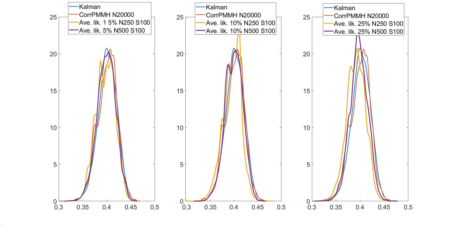
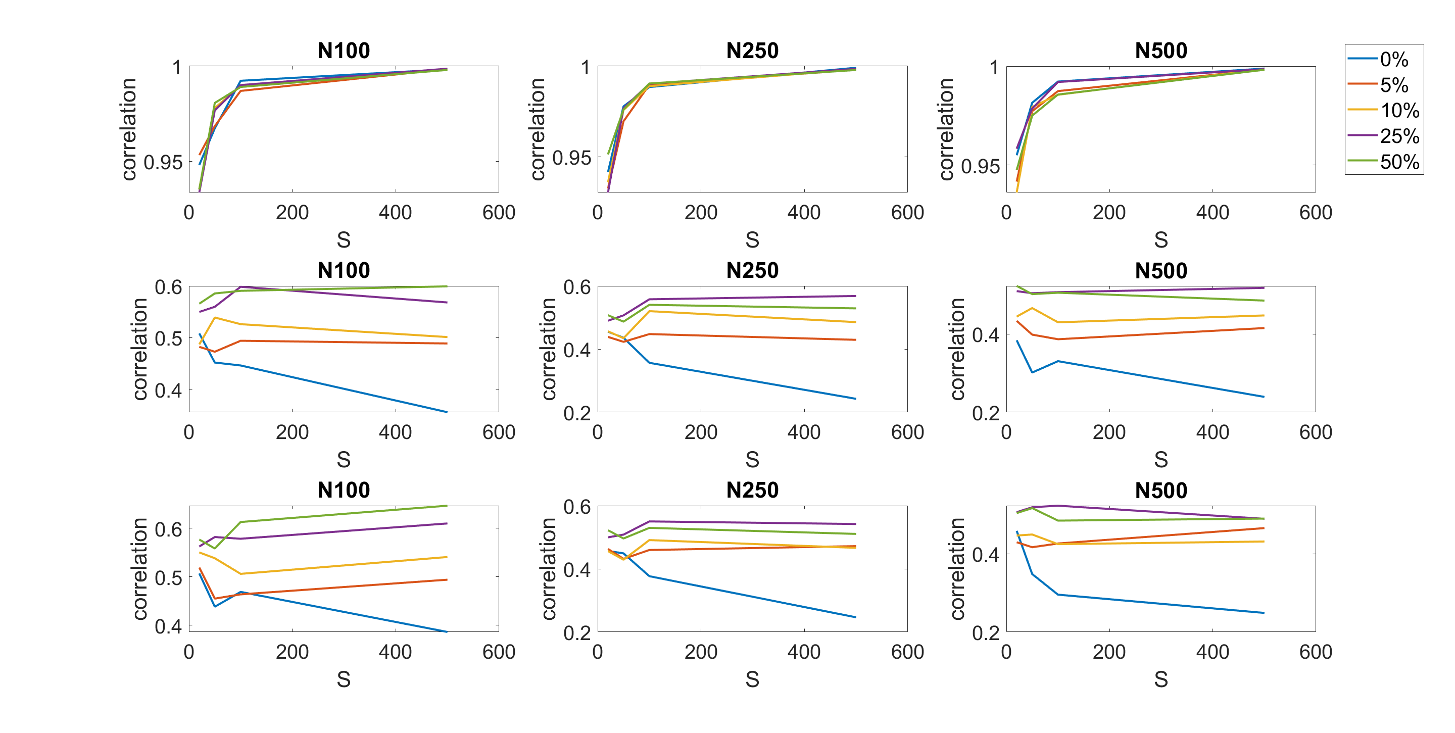
Figure S1: Left: Kernel density estimates of the parameter $\theta$ estimated using (1) Metropolis-Hastings algorithm with the (exact) Kalman filter method; (2) Correlated PMMH with $N=20000$ particles; (3) MPM with averaging the likelihood (5% trimmed mean, $S=100$, $N=250$); (4) MPM with averaging the likelihood (5% trimmed mean, $S=100$, $N=500$). Middle: Kernel density estimates of the parameter $\theta$ estimated using: (1) Metropolis-Hastings algorithm with exact Kalman filter method; (2) Correlated PMMH with 20000 particles; (3) MPM with averaging the likelihood (10% trimmed mean, $S=100$, $N=250$); (4) MPM with averaging the likelihood (10% trimmed mean, $S=100$, $N=500$). Right: Kernel density estimates of the parameter $\theta$ estimated using: (1) Metropolis-Hastings algorithm with exact Kalman filter method; (2) Correlated PMMH with 20000 particles; (3) MPM with averaging the likelihood (25% trimmed mean, $S=100$, $N=250$); (4) MPM with averaging the likelihood (25% trimmed mean, $S=100$, $N=500$) for estimating $d=10$ dimensions linear Gaussian state space model with $T=200$.

Figure S2: The estimated correlation of log of the estimated likelihoods evaluated at $\theta=0.4=\theta^{{}^{\prime}}$ (top), $\theta=0.4$ and $\theta^{{}^{\prime}}=0.399$ (middle), and $\theta=0.4$ and $\theta^{{}^{\prime}}=0.385$ (bottom) for the 10 dimensional linear Gaussian state space model with $T=300$ using the five estimators: (1) MPM (Blocking) with 0% trimmed mean of the likelihood, (2) MPM (Blocking) with 5% trimmed mean of the likelihood, (3) MPM (Blocking) with 10% trimmed mean of the likelihood, (4) MPM (Blocking) with 25% trimmed mean of the likelihood, (5) MPM (Blocking) with 50% trimmed mean of the likelihood.

Figure S2 reports the correlation estimates at the current and proposed values of $\theta$ of the log of the estimated likelihood obtained using different MPM approaches. The figure show that: (1) When the current and proposed values of the parameters are equal to $0.4$, all MPM methods maintain a high correlation between the logs of the estimated likelihoods. The estimated correlations between logs of the estimated likelihoods when the number of particle filters $S$ is 100 are about 0.99. (2) When the current parameter $\theta$ and the proposed parameter $\theta^{{}^{\prime}}$ are (slightly) different, the MPM methods can still maintain some of the correlation between the log of the estimated likelihoods. The MPM methods with 25% and 50% trimmed means of the likelihood perform the best to maintain the correlation between the logs of the estimated likelihoods.

S5 Additional tables and figures for the multivariate stochastic volatility in mean model example

This section gives additional tables and figures for the multivariate stochastic volatility in mean example in Section 3.2.

Figures S3 to S11 show the kernel density estimates of the parameters of the multivariate stochastic volatility in mean model described above estimated using the MPM sampler ($S=100$ and $N=250$) using a 25% trimmed mean with the vertical lines showing the true parameter values. The figures show that the model parameters are estimated well.

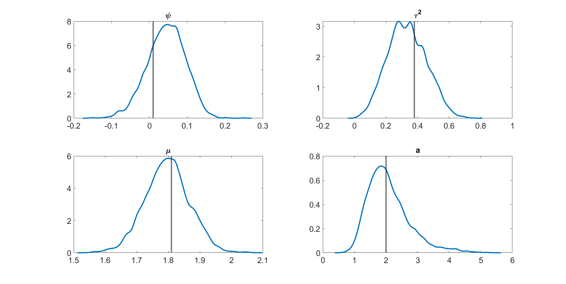
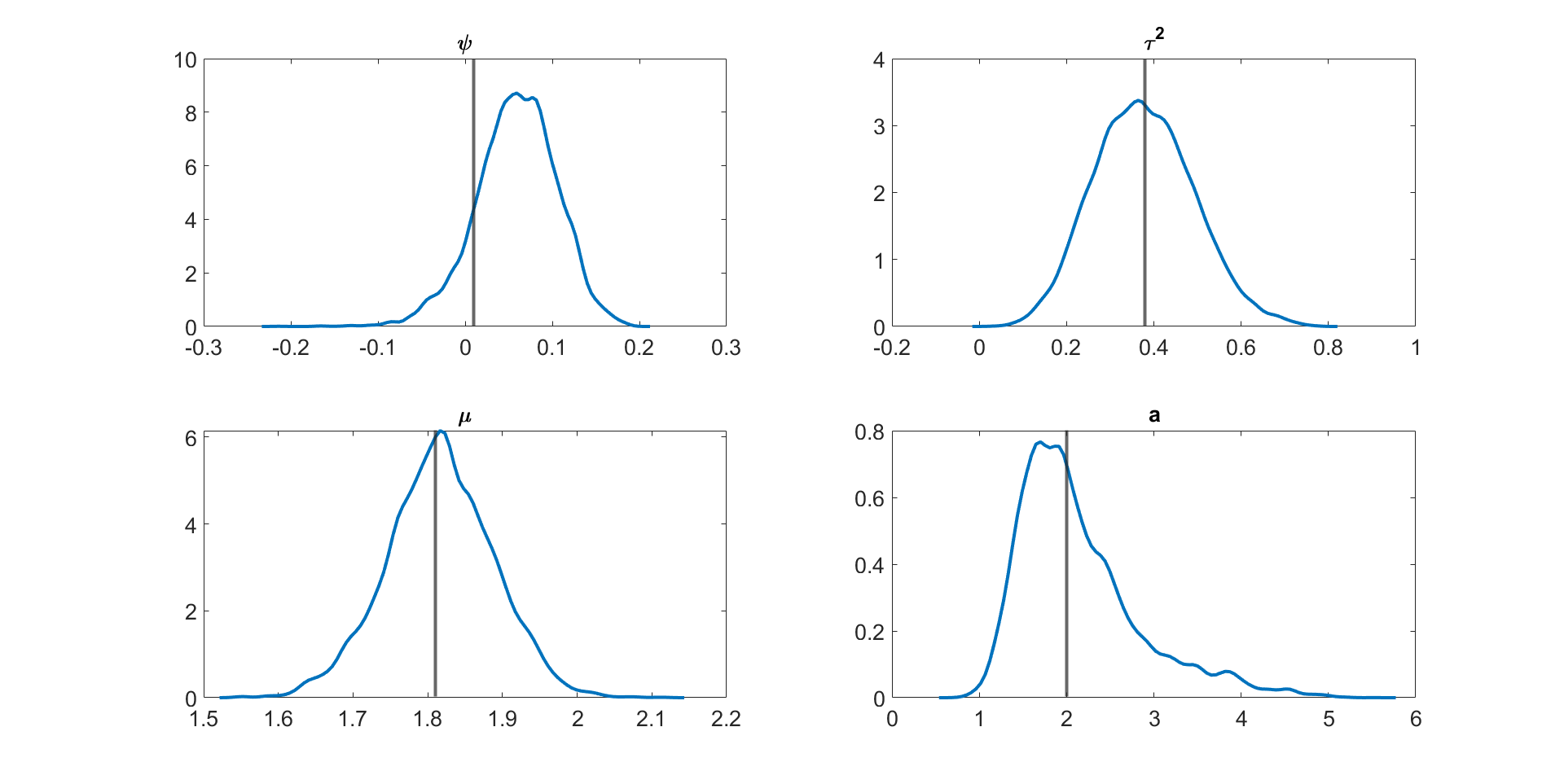
Figure S3: Kernel density estimates of the parameters of the multivariate stochastic volatility in mean model estimated using the MPM with averaging likelihood (25% trimmed mean) for a simulated dataset (data 2) with $d=20$ dimensions and $T=100$.

Figure S4: Kernel density estimates of the parameters of the multivariate stochastic volatility in mean model estimated using the MPM with averaging likelihood (25% trimmed mean) for a simulated dataset (data 3) with $d=20$ dimensions and $T=100$.

Figure S5: Kernel density estimates of the parameters of the multivariate stochastic volatility in mean model estimated using the MPM with averaging likelihood (25% trimmed mean) for a simulated dataset (data 4) with $d=20$ dimensions and $T=100$.

Figure S6: Kernel density estimates of the parameters of the multivariate stochastic volatility in mean model estimated using the MPM with averaging likelihood (25% trimmed mean) for a simulated dataset (data 5) with $d=20$ dimensions and $T=100$.

Figure S7: Kernel density estimates of the parameters of the multivariate stochastic volatility in mean model estimated using the MPM with averaging likelihood (25% trimmed mean) for a simulated dataset (data 6) with $d=20$ dimensions and $T=100$.

Figure S8: Kernel density estimates of the parameters of the multivariate stochastic volatility in mean model estimated using the MPM with averaging likelihood (25% trimmed mean) for a simulated dataset (data 7) with $d=20$ dimensions and $T=100$.

Figure S9: Kernel density estimates of the parameters of the multivariate stochastic volatility in mean model estimated using the MPM with averaging likelihood (25% trimmed mean) for a simulated dataset (data 8) with $d=20$ dimensions and $T=100$.

Figure S10: Kernel density estimates of the parameters of the multivariate stochastic volatility in mean model estimated using the MPM with averaging likelihood (25% trimmed mean) for a simulated dataset (data 9) with $d=20$ dimensions and $T=100$.

Figure S11: Kernel density estimates of the parameters of the multivariate stochastic volatility in mean model estimated using the MPM with averaging likelihood (25% trimmed mean) for a simulated dataset (data 10) with $d=20$ dimensions and $T=100$.

S6 Additional tables and figures for the small scale DSGE model example

This section gives additional tables and figures for the small scale DSGE model example in Section 3.4.1.

Table S7 gives the prior distributions for each model parameter for the non-linear small scale DSGE model in section 3.4.1. Table S8 reports the inefficiency factors for each parameter and the relative time normalised inefficiency factor (RTNIF) of a PMMH sampler relative to the MPM (0% trimmed mean) with the ADPF, disturbance sorting, and $\rho_{u}=0.99$ for the non-linear small scale models with $T=124$ time periods. Section 3.4.1 discusses the results.

Table S7: Marginal prior distributions for each model parameter for the non-linear small scale DSGE model in Section 3.4.1. The Param (1) and Param (2) columns list the mean and the standard deviation for the truncated normal (TN) and Normal distribution; $v$ and $s$ for the inverse gamma (IG) distribution. The domain $R^{+}:=(0,\infty)$. $\textrm{TN}_{\left(0,\infty\right)}$ means the normal distribution truncated to the interval $(0,\infty)$. $\textrm{TN}_{\left(0,1\right)}$ is the normal distribution truncated to the interval $(0,1)$. $\sigma^{m}_{r}$, $\sigma^{m}_{g}$, and $\sigma^{m}_{m}$ are the measurement error variances.

Param.	Domain	Density	Param (1)	Param (2)
$r^{\left(A\right)}$	$R^{+}$	$\textrm{TN}_{\left(0,\infty\right)}$	0.7	0.5
$\pi^{\left(A\right)}$	$R^{+}$	$\textrm{TN}_{\left(0,\infty\right)}$	3.12	0.5
$\gamma^{\left(Q\right)}$	$R$	N	0.60	0.5
$\tau$	$R^{+}$	$\textrm{TN}_{\left(0,\infty\right)}$	1.50	0.5
$\psi_{1}$	$R^{+}$	$\textrm{TN}_{\left(0,\infty\right)}$	2.41	0.5
$\psi_{2}$	$R^{+}$	$\textrm{TN}_{\left(0,\infty\right)}$	0.39	0.5
$\rho_{r}$	$\left[0,1\right]$	$\textrm{TN}_{\left(0,1\right)}$	0.5	0.2
$\rho_{g}$	$\left[0,1\right]$	$\textrm{TN}_{\left(0,1\right)}$	0.5	0.2
$\rho_{m}$	$\left[0,1\right]$	$\textrm{TN}_{\left(0,1\right)}$	0.5	0.2
$\sigma_{r}$	$R^{+}$	IG	5	0.5
$\sigma_{g}$	$R^{+}$	IG	5	0.5
$\sigma_{m}$	$R^{+}$	IG	5	0.5
$\sigma_{r}^{m}$	$R^{+}$	G	1	1
$\sigma_{g}^{m}$	$R^{+}$	G	1	1
$\sigma_{m}^{m}$	$R^{+}$	G	1	1

Table S8: Comparing the performance of different PMMH samplers with different number of particle filters $S$ and different number of particles $N$ in each particle filter for estimating the small scale DSGE model for the real dataset obtained from Herbst and Schorfheide, (2019) with $T=124$. Sampler I: MPM (averaging likelihood, $\rho_{u}=0.99$, disturbance sorting, ADPF). Sampler II: MPM (averaging likelihood 10% trimmed mean, $\rho_{u}=0.99$, disturbance sorting, ADPF). Sampler III: MPM (averaging likelihood 25% trimmed mean, $\rho_{u}=0.99$, disturbance sorting, ADPF). Sampler IV: MPM (averaging likelihood 25% trimmed mean, $\rho_{u}=0$, disturbance sorting, ADPF). Sampler V: MPM (averaging likelihood 25% trimmed mean, $\rho_{u}=0.99$, state sorting, ADPF). Sampler VI: DA-MPM (averaging likelihood 25% trimmed mean, $\rho_{u}=0.99$, state sorting, ADPF). Sampler VII: MPM (averaging likelihood 50% trimmed mean, $\rho_{u}=0.99$, disturbance sorting, ADPF). Sampler VIII: MPM (averaging likelihood, $\rho_{u}=0.99$, disturbance sorting, bootstrap). Sampler IX: Correlated PMMH. Time is the time in seconds for one iteration of the method.

Param	I	II	III	IV	V	VI	VII	VIII	IX
S	100	100	100	100	100	100	100	100	1
N	250	100	100	100	100	100	100	250	20000
$\pi^{\left(A\right)}$	$1477.673$	$87.796$	$87.531$	$86.956$	$97.641$	$127.836$	$95.566$	NA	$184.817$
$\tau$	$689.320$	$57.260$	$59.924$	$60.839$	$92.847$	$108.051$	$77.129$	NA	$486.328$
$\psi_{1}$	$1074.308$	$84.835$	$83.481$	$82.317$	$112.780$	$157.470$	$95.780$	NA	$313.848$
$\psi_{2}$	$645.963$	$90.750$	$96.507$	$105.948$	$148.919$	$234.819$	$116.554$	NA	$931.106$
$\gamma^{\left(Q\right)}$	$662.909$	$74.881$	$134.589$	$105.032$	$131.219$	$128.182$	$88.105$	NA	$138.769$
$r^{\left(A\right)}$	$617.848$	$110.671$	$108.337$	$79.477$	$118.001$	$156.412$	$84.812$	NA	$1463.057$
$\rho_{r}$	$651.307$	$116.273$	$113.495$	$93.525$	$135.521$	$194.771$	$118.165$	NA	$386.218$
$\rho_{g}$	$1145.901$	$152.711$	$123.128$	$99.316$	$167.833$	$604.722$	$132.060$	NA	$1064.070$
$\rho_{m}$	$864.234$	$62.183$	$110.929$	$151.060$	$96.787$	$200.407$	$236.684$	NA	$1407.105$
$\sigma_{r}$	$2254.695$	$88.552$	$104.442$	$89.854$	$142.248$	$148.776$	$94.689$	NA	$556.250$
$\sigma_{g}$	$1728.309$	$149.187$	$91.283$	$114.929$	$140.916$	$212.246$	$148.838$	NA	$676.259$
$\sigma_{m}$	$1213.429$	$87.724$	$80.627$	$72.743$	$120.432$	$195.319$	$97.566$	NA	$213.740$
$\sigma_{r}^{m}$	$1242.351$	$82.957$	$94.455$	$81.547$	$83.689$	$122.662$	$101.957$	NA	$199.629$
$\sigma_{g}^{m}$	$1078.089$	$82.678$	$66.751$	$76.764$	$81.131$	$98.441$	$79.810$	NA	$104.288$
$\sigma_{m}^{m}$	$1487.408$	$85.196$	$69.188$	$97.438$	$87.323$	$170.904$	$110.041$	NA	$1377.649$
$\widehat{\textrm{IF}}_{\psi,\textrm{MAX}}$	$2254.695$	$152.711$	$134.589$	$151.060$	$167.833$	$604.723$	$236.684$	NA	$1463.057$
$\widehat{\textrm{TNIF}}_{\textrm{MAX}}$	$2412.524$	$83.991$	$74.024$	$83.083$	$102.378$	$66.520$	$130.176$	NA	$7607.896$
$\widehat{\textrm{RTNIF}}_{\textrm{MAX}}$	$1$	$0.035$	$0.031$	$0.034$	$0.042$	$0.028$	$0.054$	NA	$3.154$
$\widehat{\textrm{IF}}_{\psi,\textrm{MEAN}}$	$1122.250$	$94.244$	$94.978$	$93.183$	$117.153$	$190.735$	$111.852$	NA	$633.542$
$\widehat{\textrm{TNIF}}_{\textrm{MEAN}}$	$1200.808$	$51.834$	$52.238$	$51.251$	$71.463$	$20.981$	$61.519$	NA	$3294.418$
$\widehat{\textrm{RTNIF}}_{\textrm{MEAN}}$	$1$	$0.043$	$0.044$	$0.043$	$0.060$	$0.017$	$0.051$	NA	$2.744$
Time	1.07	0.55	0.55	0.55	0.61	0.11	$0.55$	0.75	5.20

S7 Additional tables and figures for the medium scale DSGE model example

This section gives additional tables and figures for the medium scale DSGE model example in Section 3.4.2. Table S9 gives the prior distributions for each model parameter for the non-linear medium scale DSGE model in Section 3.4.2. Table S10 gives the mean, $2.5\%$, and $97.5\%$ quantiles estimates of each parameter in the medium scale DSGE model estimated using the MPM sampler with a $50\%$ trimmed mean ($\rho_{u}=0.99$, disturbance sorting, ADPF)) for the US quarterly dataset from 1983Q1 to 2007Q4. The measurement error variances are fixed to $25\%$ of the variance of the observables. The standard errors are relatively small for all parameters indicating that the parameters are estimated accurately.

Table S11 gives the inefficiency factor for each parameter in the medium scale DSGE model estimated using the MPM with 50% trimmed mean (ADPF, disturbance sorting, $\rho_{u}=0.9$) and the correlated PMMH samplers. Table S12 gives the mean, $2.5\%$, and $97.5\%$ quantiles estimates of each parameter in the extended version of the medium scale DSGE model estimated using the MPM sampler with a $50\%$ trimmed mean ($\rho_{u}=0.99$, disturbance sorting, ADPF)) for the US quarterly dataset from 1983Q1 to 2007Q4. The measurement error variances are fixed to $25\%$ of the variance of the observables.

Table S9: Prior distribution for each model parameter for the non-linear medium scale DSGE model. The Param (1) and Param (2) columns list the mean and the standard deviation for the truncated normal (TN) and Normal distribution; $v$ and $s$ for the shape and scale parameters of the inverse gamma (IG) and gamma (G) distribution. The domain $R^{+}:=(0,\infty)$. $\textrm{TN}_{\left(0,\infty\right)}$ means the normal distribution truncated to the interval $(0,\infty)$. $\textrm{TN}_{\left(0,1\right)}$ is the normal distribution truncated to the interval $(0,1)$. $\sigma_{r}^{m}$, $\sigma_{g}^{m}$, and $\sigma_{m}^{m}$ are the measurement error variances.

Param.	Domain	Density	Param. (1)	Param. (2)
$\rho_{R}$	$\left[0,1\right]$	$\textrm{TN}_{\left[0,1\right]}$	$0.6$	$0.2$
$\rho_{g}$	$\left[0,1\right]$	$\textrm{TN}_{\left[0,1\right]}$	$0.6$	$0.2$
$\rho_{\mu}$	$\left[0,1\right]$	$\textrm{TN}_{\left[0,1\right]}$	$0.6$	$0.2$
$100\sigma_{g}$	$R^{+}$	G	$0.5$	$0.5$
$100\sigma_{\mu}$	$R^{+}$	G	$0.5$	$0.5$
$100\sigma_{\eta}$	$R^{+}$	G	$0.5$	$0.5$
$100\sigma_{Z}$	$R^{+}$	G	$0.5$	$0.5$
$100\sigma_{R}$	$R^{+}$	G	$0.5$	$0.5$
$100\sigma_{gdp}$	$R^{+}$	G	$0.5$	$0.5$
$100\sigma_{con}$	$R^{+}$	G	$0.5$	$0.5$
$100\sigma_{inv}$	$R^{+}$	G	$0.5$	$0.5$
$100\sigma_{inf}$	$R^{+}$	G	$0.5$	$0.5$
$100\sigma_{ffr}$	$R^{+}$	G	$0.5$	$0.5$
$\gamma_{g}$	$R$	N	$0.4$	$0.2$
$\gamma_{\Pi}$	$R$	N	$1.7$	$0.3$
$\gamma_{x}$	$R$	N	$0.4$	$0.3$
$\gamma$	$\left[0,1\right]$	$\textrm{TN}_{\left[0,1\right]}$	$0.6$	$0.1$
$\sigma_{a}$	$R^{+}$	G	$25$	$0.2$
$\varphi_{p}/100$	$R$	N	$1$	$0.25$
$\varphi_{w}/1000$	$R$	N	$3$	$5$
$\varphi_{I}$	$R^{+}$	G	$16$	$0.25$
$\sigma_{L}$	$R^{+}$	G	$5.34$	$0.37$
$1-a$	$\left[0,1\right]$	$\textrm{TN}_{\left[0,1\right]}$	$0.5$	$0.15$
$1-a_{w}$	$\left[0,1\right]$	$\textrm{TN}_{\left[0,1\right]}$	$0.5$	$0.15$
$100\left(\beta^{-1}-1\right)$	$R^{+}$	G	$0.625$	$4$
$100\log\left(G_{z}\right)$	$R$	N	$0.5$	$0.03$
$100\left(\overline{\Pi}-1\right)$	$R$	N	$0.62$	$0.1$
$\alpha$	$R$	N	$0.3$	$0.05$

Table S10: Posterior means, $2.5\%$, and $97.5\%$ quantiles of the posterior distributions of each of the parameters in the medium scale DSGE model estimated using the MPM sampler with $50\%$ trimmed mean ($\rho_{u}=0.99$, disturbance sorting, ADPF)) for the US quarterly dataset from 1983Q1 to 2007Q4. The measurement error variances are fixed to $25\%$ of the variance of the observables. The standard errors in brackets are calculated from $10$ independent runs of the MPM sampler

Param.	Estimates	$2.5\%$	$97.5\%$
$\rho_{R}$	$\underset{\left(0.0178\right)}{0.4329}$	$\underset{\left(0.0365\right)}{0.2097}$	$\underset{\left(0.0220\right)}{0.6490}$
$\rho_{g}$	$\underset{\left(0.0008\right)}{0.9883}$	$\underset{\left(0.0020\right)}{0.9770}$	$\underset{\left(0.0005\right)}{0.9965}$
$\rho_{\mu}$	$\underset{\left(0.0191\right)}{0.5975}$	$\underset{\left(0.0309\right)}{0.4136}$	$\underset{\left(0.0410\right)}{0.7598}$
$100\sigma_{g}$	$\underset{\left(0.0104\right)}{0.2188}$	$\underset{\left(0.0129\right)}{0.0973}$	$\underset{\left(0.0182\right)}{0.3992}$
$100\sigma_{\mu}$	$\underset{\left(0.0978\right)}{4.1832}$	$\underset{\left(0.2905\right)}{2.1935}$	$\underset{\left(0.2697\right)}{7.0727}$
$100\sigma_{\eta}$	$\underset{\left(0.0096\right)}{0.3614}$	$\underset{\left(0.0082\right)}{0.2706}$	$\underset{\left(0.0151\right)}{0.4837}$
$100\sigma_{Z}$	$\underset{\left(0.0118\right)}{0.6240}$	$\underset{\left(0.0168\right)}{0.4707}$	$\underset{\left(0.0121\right)}{0.7954}$
$100\sigma_{R}$	$\underset{\left(0.0032\right)}{0.0462}$	$\underset{\left(0.0002\right)}{0.0059}$	$\underset{\left(0.0123\right)}{0.1570}$
$\gamma_{g}$	$\underset{\left(0.0162\right)}{0.3051}$	$\underset{\left(0.0130\right)}{0.0435}$	$\underset{\left(0.0541\right)}{0.7360}$
$\gamma_{\Pi}$	$\underset{\left(0.0039\right)}{0.9897}$	$\underset{\left(0.0146\right)}{0.9671}$	$\underset{\left(0.0016\right)}{1.0072}$
$\gamma_{x}$	$\underset{\left(0.0115\right)}{0.7649}$	$\underset{\left(0.0106\right)}{0.4726}$	$\underset{\left(0.0428\right)}{1.0829}$
$\gamma$	$\underset{\left(0.0086\right)}{0.4606}$	$\underset{\left(0.0131\right)}{0.3506}$	$\underset{\left(0.0128\right)}{0.5727}$
$\sigma_{a}$	$\underset{\left(0.1244\right)}{4.9188}$	$\underset{\left(0.1777\right)}{3.4442}$	$\underset{\left(0.2509\right)}{6.7495}$
$\varphi_{p}$	$\underset{\left(3.6050\right)}{86.7032}$	$\underset{\left(15.1263\right)}{37.4987}$	$\underset{\left(3.4207\right)}{138.1528}$
$\varphi_{w}$	$\underset{\left(289.8829\right)}{2879.123}$	$\underset{\left(110.8468\right)}{1230.612}$	$\underset{\left(856.0024\right)}{5076.731}$
$\varphi_{I}$	$\underset{\left(0.0798\right)}{2.4537}$	$\underset{\left(0.0887\right)}{1.4166}$	$\underset{\left(0.2252\right)}{3.9636}$
$\sigma_{L}$	$\underset{\left(0.1389\right)}{3.8518}$	$\underset{\left(0.1179\right)}{2.0824}$	$\underset{\left(0.2504\right)}{6.1554}$
$1-a$	$\underset{\left(0.0140\right)}{0.4386}$	$\underset{\left(0.0351\right)}{0.2153}$	$\underset{\left(0.0355\right)}{0.7024}$
$1-a_{w}$	$\underset{\left(0.0119\right)}{0.6493}$	$\underset{\left(0.0236\right)}{0.3875}$	$\underset{\left(0.0074\right)}{0.8285}$
$100\left(\beta^{-1}-1\right)$	$\underset{\left(0.0187\right)}{0.0651}$	$\underset{\left(0.0034\right)}{0.0052}$	$\underset{\left(0.0866\right)}{0.2034}$
$100\log\left(G_{z}\right)$	$\underset{\left(0.0035\right)}{0.5144}$	$\underset{\left(0.0039\right)}{0.4650}$	$\underset{\left(0.0042\right)}{0.5708}$
$100\left(\overline{\Pi}-1\right)$	$\underset{\left(0.0069\right)}{0.6150}$	$\underset{\left(0.0132\right)}{0.4213}$	$\underset{\left(0.0164\right)}{0.7977}$
$\alpha$	$\underset{\left(0.0032\right)}{0.1738}$	$\underset{\left(0.0064\right)}{0.1284}$	$\underset{\left(0.0034\right)}{0.2151}$

Table S11: Comparing the performance of different PMMH samplers with different number of particle filters $S$ and different number of particles $N$ in each particle filter for estimating the medium scale DSGE model using the US quarterly dataset from 1983Q1 to 2007Q4. Sampler I: MPM (50% trimmed mean, $\rho_{u}=0.9$, disturbance sorting, ADPF). Sampler II: Correlated PMMH. The first two columns are the inefficiency factors of each parameter for the case when the measurement error variances are estimated. The last two columns are the inefficiency factor of each parameter for the case when the measurement error variances are fixed at 25% of the variance of each observable over the estimation period.

Param.	I	II	I	II
$\rho_{R}$	$450.704$	$1886.791$	$318.305$	$277.221$
$\rho_{g}$	$523.660$	$653.350$	$205.736$	$292.167$
$\rho_{\mu}$	$618.928$	$1354.582$	$233.298$	$238.901$
$100\sigma_{g}$	$593.827$	$1731.764$	$286.744$	$302.512$
$100\sigma_{\mu}$	$396.348$	$1239.142$	$335.987$	$173.760$
$100\sigma_{\eta}$	$380.984$	$634.356$	$234.383$	$203.419$
$100\sigma_{Z}$	$456.971$	$1035.444$	$263.295$	$226.536$
$100\sigma_{R}$	$412.131$	$1008.377$	$247.562$	$214.989$
$100\sigma_{gdp}$	$372.244$	$621.6010$	NA	NA
$100\sigma_{con}$	$364.200$	$1272.367$	NA	NA
$100\sigma_{inv}$	$287.053$	$1024.054$	NA	NA
$100\sigma_{inf}$	$353.456$	$1395.761$	NA	NA
$100\sigma_{ffr}$	$292.713$	$1309.101$	NA	NA
$\gamma_{g}$	$279.772$	$1512.739$	$243.631$	$244.901$
$\gamma_{\Pi}$	$794.587$	$842.370$	$367.625$	$441.666$
$\gamma_{x}$	$361.702$	$1210.535$	$308.195$	$280.568$
$\gamma$	$365.017$	$1175.542$	$208.171$	$269.869$
$\sigma_{a}$	$379.348$	$1939.116$	$241.076$	$247.873$
$\varphi_{p}/100$	$393.882$	$1036.088$	$245.650$	$175.856$
$\varphi_{w}/1000$	$462.727$	$1222.371$	$341.178$	$568.954$
$\varphi_{I}$	$371.357$	$1004.829$	$299.040$	$242.744$
$\sigma_{L}$	$426.799$	$926.466$	$230.927$	$242.741$
$1-a$	$434.454$	$1566.728$	$251.796$	$237.491$
$1-a_{w}$	$359.744$	$839.328$	$255.983$	$229.476$
$100\left(\beta^{-1}-1\right)$	$796.824$	$660.065$	$383.310$	$343.446$
$100\log\left(G_{z}\right)$	$336.080$	$2181.566$	$252.953$	$203.629$
$100\left(\overline{\Pi}-1\right)$	$295.468$	$967.840$	$259.442$	$202.170$
$\alpha$	$442.753$	$1120.534$	$318.548$	$224.703$

Table S12: Posterior means, $2.5\%$, and $97.5\%$ quantiles of the posterior distributions, and the inefficiency factors of each of the parameters in the extended version of the medium scale DSGE model estimated using the MPM sampler with $50\%$ trimmed mean ($\rho_{u}=0.99$, disturbance sorting, ADPF)) for the US quarterly dataset from 1983Q1 to 2007Q4. The measurement error variances are fixed to $25\%$ of the variance of the observables.

Param.	Estimates	$2.5\%$	$97.5\%$	$\widehat{\textrm{IF}}$
$\rho_{R}$	$0.522$	$0.204$	$0.759$	$229.752$
$\rho_{g}$	$0.608$	$0.241$	$0.929$	$201.565$
$\rho_{\mu}$	$0.560$	$0.383$	$0.723$	$170.293$
$100\sigma_{g}$	$0.052$	$0.006$	$0.157$	$151.086$
$100\sigma_{\mu}$	$4.085$	$2.494$	$6.047$	$169.246$
$100\sigma_{\eta}$	$0.350$	$0.262$	$0.468$	$220.044$
$100\sigma_{Z}$	$0.628$	$0.483$	$0.800$	$203.168$
$100\sigma_{R}$	$0.102$	$0.007$	$0.238$	$185.973$
$\gamma_{g}$	$0.354$	$-0.019$	$0.856$	$209.208$
$\gamma_{\Pi}$	$1.011$	$1.001$	$1.032$	$301.381$
$\gamma_{x}$	$0.878$	$0.506$	$1.314$	$266.684$
$\gamma$	$0.457$	$0.330$	$0.588$	$199.630$
$\sigma_{a}$	$5.596$	$3.798$	$7.694$	$167.707$
$\varphi_{p}$	$65.973$	$17.465$	$118.752$	$250.439$
$\varphi_{w}$	$814.476$	$263.520$	$1911.136$	$310.302$
$\varphi_{I}$	$2.292$	$1.223$	$3.663$	$193.898$
$\sigma_{L}$	$5.212$	$2.946$	$7.784$	$203.591$
$1-a$	$0.326$	$0.087$	$0.545$	$164.680$
$1-a_{w}$	$0.613$	$0.273$	$0.862$	$257.090$
$100\left(\beta^{-1}-1\right)$	$0.094$	$0.006$	$0.315$	$223.610$
$100\log\left(G_{z}\right)$	$0.518$	$0.468$	$0.568$	$176.914$
$100\left(\overline{\Pi}-1\right)$	$0.611$	$0.429$	$0.795$	$154.344$
$\alpha$	$0.181$	$0.137$	$0.221$	$165.125$

S8 Description: Small scale DSGE model

The small scale DSGE model specification follows Herbst and Schorfheide, (2016), and is also used by Herbst and Schorfheide, (2019). The small scale DSGE model follows the environment in Herbst and Schorfheide, (2019) with nominal rigidities through price adjustment costs following Rotemberg, (1982), and three structural shocks. There are altogether $4$ state variables, $4$ control variables ($8$ variables combining the state and control variables) and $3$ exogenous shocks in the model. We estimate this model using $3$ observables; that means that the dimensions of $y_{t}$, the state vector and the disturbance vector are $3$, $8$, and $3$, respectively.

Households

Time is discrete, households live forever, the representative household derives utility from consumption $C_{t}$ relative to a habit stock (which is approximated by the level of technology $A_{t}$) and real money balances $\frac{M_{t}}{P_{t}}$ and disutility from hours worked $N_{t}$. The household maximizes

$$E_{0}\sum_{t=0}^{\infty}\beta^{t}\Big{[}\frac{\big{(}\frac{C_{t}}{A_{t}}\big{)}^{1-\tau}-1}{1-\tau}+\chi_{M}\log\frac{M_{t}}{P_{t}}-\chi_{N}{N_{t}}\Big{]}$$

subject to the budget constraint

$$P_{t}C_{t}+B_{t}+M_{t}+T_{t}=P_{t}W_{t}N_{t}+R_{t-1}B_{t-1}+M_{t-1}+P_{t}D_{t}+P_{t}{SC}_{t};$$

$T_{t},D_{t}$ and ${SC}_{t}$ denote lump-sum taxes, aggregate residual profits and net cash inflow from trading a full set of state contingent securities; $P_{t}$ is the aggregate price index, and $W_{t}$ is the real wage; $\beta$ is the discount factor, ${\tau}$ is the coefficient of relative risk aversion, $\chi_{M}$ and $\chi_{N}$ are scale factors determining the steady state money balance holdings and hours. We set $\chi_{N}=1$. $A_{t}$ is the level of aggregate productivity.

Firms

Final output is produced by a perfectly competitive representative firm which uses a continuum of intermediate goods $Y_{t}(i)$ and the production function

$${Y_{t}}=\Bigg{(}\int_{0}^{1}Y_{t}(i)^{1-\nu}di\Bigg{)}^{\frac{1}{1-\nu}},$$

with $\nu<1$. The demand for intermediate good $i$ is

$$Y_{t}(i)=\Bigg{(}\frac{P_{t}(i)}{P_{t}}\Bigg{)}^{-\frac{1}{\nu}}Y_{t},$$

and the aggregate price index is

$$P_{t}=\Bigg{(}\int_{0}^{1}P_{t}(i)^{\frac{\nu-1}{\nu}}di\Bigg{)}^{\frac{\nu}{\nu-1}}.$$

Intermediate good $i$ is produced using the linear production technology

$$Y_{t}(i)=A_{t}N_{t}(i);$$

$A_{t}$ is an exogenous productivity process common to all firms, and $N_{t}(i)$ is the labor input of firm i. Intermediate firms set prices $(P_{t}(i))$ and labor input ($N_{t}(i)$) by maximizing the net present value of future profit. Nominal rigidities are introduced through price adjustment costs following Rotemberg, (1982).

$$E_{t}\sum_{s=0}^{\infty}\beta^{s}Q_{t,t+s}\Big{[}\frac{P_{t+s(i)}}{P_{t+s}}Y_{t+s}(i)-W_{t+s}N_{t+s}(i)-AC_{t+s}(i)\Big{]}$$

with

$$AC_{t}(i)=\frac{\phi}{2}\Bigg{(}\frac{P_{t}(i)}{P_{t-1}(i)}-\pi\Bigg{)}^{2}{Y_{t}(i)}$$

The parameter $\phi$ governs the extent of price rigidity in the economy and $\pi$ is the steady state inflation rate associated with the final good. In equilibrium, households and firms use the same stochastic discount factor $Q_{t,t+s}$ where

$$Q_{t,t+s}=\Big{(}\frac{C_{t+s}}{C_{t}}\Big{)}^{-\tau}{\Big{(}\frac{A_{t}}{A_{t+s}}\Big{)}^{1-\tau}}.$$

In a symmetric equilibrium all firms choose the same price.

Monetary and Fiscal Policy

The central bank conducts monetary policy following an interest rate feedback rule given by

$$R_{t}={R_{t}^{*}}^{1-\rho_{R}}R_{t-1}^{\rho_{R}}\epsilon_{t}^{R},$$

where $\epsilon_{t}^{R}\sim IID({0,\sigma_{r}})$ is an iid shock to the nominal interest rate, ${R_{t}^{*}}$ is the nominal target and $(1-\rho_{R})$ captures interest rate smoothing in the conduct of policy,

$${R_{t}^{*}}=r\pi^{*}\Big{(}\frac{\pi_{t}}{\pi^{*}}\Big{)}^{\psi_{1}}\Big{(}\frac{Y_{t}}{Y_{t}^{*}}\Big{)}^{\psi_{2}};$$

$\pi_{t}:=\frac{P_{t}}{P_{t-1}}$ is the gross inflation rate and $\pi^{*}$ is the target inflation rate. $Y_{t}^{*}$ is the output in the absence of nominal rigidities. The parameters $\psi_{1}$ and $\psi_{2}$ capture the intensity with which the central bank responds to inflation and output gap in the model. Government expenditure accounts for a fraction $\upsilon_{t}\in[0,1]$ of final output such that $G_{t}=\upsilon_{t}Y_{t}$. The government budget constraint is

$$P_{t}G_{t}+R_{t-1}B_{t-1}+M_{t-1}=T_{t}+B_{t}+M_{t}.$$

Aggregation

Combining the household budget constraint with the government budget constraint gives

$$C_{t}+G_{t}+AC_{t}=Y_{t}$$

where in equilibrium, $AC_{t}=\frac{\phi}{2}(\pi_{t}-\pi)^{2}{Y}_{t}$.

Exogenous Processes

Aggregate technology grows at the rate $\gamma$ and $m_{t}$ is the shock to aggregate demand such that

$$\log{A_{t}}=\log{\gamma}+\log{A_{t-1}}+\log{m_{t}}$$

$$\log{m_{t}}=(1-\rho_{m})\log{m}+\rho_{m}\log{m_{t-1}}+\epsilon_{t}^{m}$$

with $\epsilon_{t}^{m}\sim IID({0,\sigma_{m}})$. We define $g_{t}:=1/(1-\upsilon_{t})$ and $g_{t}$ evolves as

$$\log{g_{t}}=(1-\rho_{g})\log{g}+\rho_{g}\log{g_{t-1}}+\epsilon_{t}^{g},$$

with $\epsilon_{t}^{g}\sim IID({0,\sigma_{g}})$. We summarize the nonlinear equilibrium conditions after detrending $C_{t},Y_{t},G_{t}$ by deterministic technology, i.e define $\tilde{X_{t}}:=X_{t}/A_{t}$:

$$1=\beta{E_{t}}\Big{[}\bigg{(}\frac{\tilde{C}_{t+1}}{\tilde{C}_{t}}\bigg{)}^{-\tau}{z_{t}}\frac{R_{t}}{\pi_{t+1}}\Big{]}$$ (S10)

$$1=\phi(\pi_{t}-\pi)\Big{[}\bigg{(}1-\frac{1}{2\nu}\bigg{)}\pi_{t}+\frac{\pi}{2\nu}\Big{]}-\phi{E_{t}}\Big{[}\bigg{(}\frac{\tilde{C}_{t+1}}{\tilde{C}_{t}}\bigg{)}^{-\tau}\frac{\tilde{Y}_{t+1}}{\tilde{Y}_{t}}(\pi_{t+1}-\pi)\pi_{t+1}\Big{]}+\frac{1}{\nu}\Big{[}1-\bigg{(}{\tilde{C}_{t}}\bigg{)}^{\tau}\Big{]}$$

$$R_{t}={R_{t}^{*}}^{1-\rho_{R}}R_{t-1}^{\rho_{R}}\exp{\epsilon_{t}^{R}}$$

$${R_{t}^{*}}=r\pi^{*}\Big{(}\frac{\pi_{t}}{\pi^{*}}\Big{)}^{\psi_{1}}\Big{(}\frac{\tilde{Y}_{t}}{\tilde{Y}_{t}^{*}}\Big{)}^{\psi_{2}}$$

$$\tilde{C}_{t}+\tilde{G}_{t}+\frac{\phi}{2}(\pi_{t}-\pi)^{2}\tilde{Y}_{t}=\tilde{Y}_{t}$$

$$\log{A_{t}}=\log{\gamma}+\log{A_{t-1}}+\log{m_{t}}$$

$$\log{m_{t}}=(1-\rho_{m})\log{m}+\rho_{m}\log{m_{t-1}}+\epsilon_{t}^{m}$$ (S11)

$$\log{g_{t}}=(1-\rho_{g})\log{g}+\rho_{g}\log{g_{t-1}}+\epsilon_{t}^{g}.$$ (S12)

After detrending, the steady state solution of the model is $\pi=\pi^{*},\tilde{R}=\frac{\gamma\pi}{\beta},\tilde{C}=(1-\nu)^{\frac{1}{\tau}}\;\;\mathrm{and}\;\;\tilde{Y}=g\tilde{C}=\tilde{y^{*}}$.

Equations (S10)-(S12) can now be rewritten as

$$E_{t}G(z_{t+1},z_{t},\epsilon_{t+1})=0,$$

where

$$z_{t}=[\tilde{C}_{t},\tilde{Y}_{t},\tilde{G}_{t},R_{t},R_{t}^{*},A_{t},m_{t},g_{t}]\quad\text{and}\quad\epsilon_{t}=[\epsilon_{t}^{R},\epsilon_{t}^{m},\epsilon_{t}^{g}],$$

and solved using the methods in Section  S3.

We solve the model in log deviations from steady state, i.e. $\widehat{x_{t}}:=\log\Big{(}\frac{\tilde{X_{t}}}{\tilde{X}}\Big{)}$ using Dynare. The small scale DSGE model therefore consists of a consumption Euler equation, a new Keynesian Philip curve, a monetary policy rule, fiscal policy rule, three exogenous shock processes, and eight endogenous latent variables. We estimate the model using both first and second order approximations to assess the performance of our proposed method relative to existing methods. As explained, the source of nonlinearity in our case stems from taking a second order approximation of the equilibrium conditions.

The observables used in estimating the model consist of per capita GDP growth rate ($YGR_{t}$), annualized quarter on quarter inflation rate ($Infl_{t}$) and annualized nominal rates ($Int_{t}$). The observed data is measured in percentages, and, after applying a log transformation to the endogenous variables, the measurement equations for our system using the transformed endogenous variables given by (a hatted variable denotes the log transformation).

$$YGR_{t}=\gamma^{(Q)}+100(\hat{y}_{t}-\hat{y}_{t-1}+\hat{m}_{t}),$$

$$Infl_{t}=\pi^{(A)}+400\hat{\pi}_{t},$$

$$Int_{t}=\pi^{(A)}+r^{(A)}+4\gamma^{(Q)}+400\hat{R}_{t}.$$

Here, $\hat{y}_{t}=\log\Big{(}\frac{\tilde{Y_{t}}}{\tilde{Y}}\Big{)}$, $\hat{\pi}_{t}=\log\Big{(}\frac{\pi_{t}}{{\pi}}\Big{)}$, $\hat{R}_{t}=\log\Big{(}\frac{R_{t}}{{\overline{R}}}\Big{)}$ and $\hat{m}_{t}=\log\Big{(}\frac{m_{t}}{{\overline{m}}}\Big{)}=\log{m_{t}}$ since $\log(\overline{m})=0$ in steady state as evident from Equation (S11).

The model has the 15 parameters

$$\Big{\{}\upsilon,\nu,\phi,\tau,\pi^{\left(A\right)},r^{\left(A\right)},\gamma^{\left(Q\right)},\psi_{1},\psi_{2},\rho_{r},\rho_{g},\rho_{m},\sigma_{r},\sigma_{g},\sigma_{m}\Big{\}}.$$

We calibrate the parameters characterizing the share of fiscal expenditure in GDP $\upsilon=0.2$, the elasticity of substitution across varieties $1/\nu=11$ and the parameter guiding the extent of nominal rigidities, $\phi=100$. The remaining parameters along with the measurement errors in the observation equation are estimated. The steady-state inflation rate, $\pi$, in the model relates to the estimated parameter for annualized inflation $\pi^{(A)}$ such that $\pi=\pi^{(A)}/400$ and the discount factor $\beta$ to the estimated parameter for annualized interest rate $r^{(A)}$ such that $\beta=\Big{(}(1+r^{(A)})/400\Big{)}^{-1}$. The sample used for estimation is 1983Q1-2002Q4. The data set and the variables are identical to those used in Herbst and Schorfheide, (2019).

S9 Description: Medium scale DSGE model

The specification of the medium-scale model is similar to Smets and Wouters, (2007) and follows the specification in Gust et al., (2017). The model allows for habit formation in consumption, nominal rigidities in wages and prices, indexation in wages and prices, and investment adjustment costs. The model environment consists of monopolistically competitive intermediate goods-producing firms, a perfectly competitive final good-producing firm, households, and the government conducting fiscal and monetary policy. We describe the behavior of each agent in detail below. The baseline model in Gust et al., (2017) consists of 12 state variables, 18 control variables (30 variables combining the state and control variables) and 5 exogenous shocks. We estimate this model using 5 observables; that means that the dimensions of $y_{t}$, the state vector and the disturbance vector are $5$, $30$, and $5$, respectively. We also consider a variation of the medium scale DSGE model of Gust et al., (2017). To study how well our approach performs with increasing state dimension, we estimate the model with the canonical definition of the output gap defined as the difference between output in the model with nominal rigidities and output in the model with flexible prices and wages. This variation is identical to the baseline model in Gust et al., (2017) except for the Taylor rule specification, which now uses the canonical definition of the output gap. This extension of the medium scale DSGE model consists of 21 state variables, 30 control variables (51 variables combining the state and control variables) and 5 exogenous shocks. We estimate this model using 5 observables; that means that the dimensions of $y_{t}$, the state vector and the disturbance vector are $5$, $51$, and $5$, respectively.

S9.1 Firms

There is a continuum of monopolistically competitive firms producing differentiated intermediate goods. The final good ($Y_{t}$) is produced by a perfectly competitive representative firm that uses a continuum of differentiated intermediate goods ($Y_{t}(i)$) such that

$${Y_{t}}=\Bigg{(}\int_{0}^{1}Y_{t}(j)^{\frac{\epsilon_{p}-1}{\epsilon_{p}}}dj\Bigg{)}^{\frac{\epsilon_{p}}{\epsilon_{p}-1}}.$$

Under the constant elasticity of substitution aggregator, the demand for good produced by the $j^{th}$ firm is

$$Y_{t}(j)=\Bigg{(}\frac{P_{t}(j)}{P_{t}}\Bigg{)}^{-\epsilon_{p}}Y_{t},$$

The production function for the $j^{th}$ intermediate good producer is

$${Y_{t}(j)}=K_{t}(j)^{\alpha}(Z_{t}N_{t}(j))^{(1-\alpha)}.$$

$N_{t}(j)$ and $K_{t}(j)$ denote labor and capital inputs for the $j^{th}$ intermediate good producer and $Z_{t}$ denotes labor augmenting technological progress. $Z_{t}$ evolves as

$$Z_{t}=Z_{t-1}G_{z}\exp(\epsilon_{z,t});\text{ }\epsilon_{z,t}\overset{iid}{\sim}N(0,\sigma_{z}^{2});$$

$G_{z}$ is the deterministic growth rate of technology and $\epsilon_{z,t}$ introduces deviations about this deterministic trend. Following Rotemberg, (1982), intermediate good producing firm $j$ face quadratic costs in adjusting nominal prices $P_{t}(j)$ and is given by

$$\frac{\phi_{p}}{2}\Bigg{(}\frac{P_{t}(j)}{\tilde{\pi}_{t-1}P_{t-1}(j)}-1\Bigg{)}^{2}{Y_{t}}$$

with $\phi_{p}$ describes the size of adjustment cost. The change in price is indexed to $\tilde{\pi}_{t-1}$ with

$$\tilde{\pi}_{t-1}=\overline{\pi}^{a}{{\pi}_{t-1}^{1-a}}.$$

Here $\overline{\pi}$ is the inflation target set by the central bank and ${\pi}_{t-1}:=\frac{P_{t-1}}{P_{t-2}}$ is the lagged gross inflation in period $t-1$. The parameter $a$ quantifies the extent of indexation to the central bank inflation target or lagged gross inflation with $a\in[0,1]$. The optimal price is set by each intermediate good producing firm by maximizing the expected present discounted value of profits

$$E_{t}\sum_{s=0}^{\infty}\frac{\Lambda_{t+s}}{\Lambda_{t}}\Big{[}\Big{(}\frac{P_{t+s}(j)}{P_{t+s}}-mc_{t+s}\Big{)}Y_{t+s}(j)-\frac{\psi_{p}}{2}\Big{(}\frac{P_{t+s}(j)}{\tilde{\pi}_{{t+s}-1}P_{{t+s}-1}(j)}-1\Big{)}^{2}{Y_{t+s}}\Big{]};$$

$mc_{t}$ is the real marginal cost with $mc_{t}:=\frac{{(W_{t}/P_{t})}^{1-\alpha}{(R_{t}^{K}/P_{t})}^{\alpha}}{\alpha^{\alpha}{1-\alpha}^{1-\alpha}}$. $W_{t}$ and $R_{t}^{K}$ denote the nominal wage and nominal rental rate of capital services respectively. $\frac{\Lambda_{t+s}}{\Lambda_{t}}$ is the stochastic discount factor from the optimization exercise of households.

S9.2 Households

There exists a continuum of infinitely lived monopolistically competitive households indexed by $i\in[0,1]$ supplying differentiated labor service, $N_{t}(i)$. Household $i$ sells labor service $N_{t}(i)$ to a representative employment agency which combines the differentiated labor services across the spectrum of households into a composite $N_{t}$, which in turn is supplied to the intermediate goods producers for production in a perfectly competitive market. Differentiated labor services is aggregated via a Dixit-Stiglitz aggregator given by

$$N_{t}=\Big{(}\int_{0}^{1}N_{t}(i)^{\frac{\epsilon_{w}-1}{\epsilon_{w}}}di\Big{)}^{\frac{\epsilon_{w}}{\epsilon_{w}-1}}.$$

The parameter $\epsilon_{w}$ is the constant elasticity of substitution across different varieties of labor services. Households maximize lifetime utility,

$$E_{0}\sum_{t=0}^{\infty}\beta^{t}\Big{[}\Big{(}C_{t}(i)-\gamma C_{t-1}(i)\Big{)}-\psi_{L}\frac{N_{t}(i)^{1+\sigma_{L}}}{1+\sigma_{L}}-\psi_{t}^{w}(i)\Big{]},$$

with $C_{t+s}(i)$ consumption, $N_{t+s}(i)$ being labor services, and $\psi_{t}^{w}(i)$ denotes the loss in utility due to adjusting nominal wages $W_{t}(i)$. The utility cost of adjusting nominal wages is quadratic. The cost of adjusting nominal wages is

$$\psi_{t}^{w}(i)=\frac{\phi_{w}}{2}\Bigg{(}\frac{W_{t}(j)}{\tilde{\pi}_{t-1}^{w}W_{t-1}(j)}-1\Bigg{)}^{2}.$$

The parameter $\phi_{w}$ governs the size of wage adjustment costs. Wage contracts are indexed to productivity and inflation with

$$\tilde{\pi}_{t}^{w}=G_{z}\overline{\pi}^{a_{w}}(\exp(\epsilon_{z},t)\pi_{t-1})^{1-a_{w}}.$$

The parameter $\gamma$ governs the degree of habit formation in household utility. Households also engage in savings. Households can save by investing in risk-free nominal bonds ($B_{t+s}(i)$) and owning physical capital stock $\overline{K}_{t}(i)$. Additionally, households can choose the extent of capital utilization $u_{t}(i)$. Utilization is combined with physical capital stock to transform physical capital to capital services $K_{t}(i)=u_{t}(i)\overline{K}_{t}(i)$. In the process of transforming physical capital to capital services via utilization $u_{t}(i)$, households incur costs of utilization

$$a(u_{t}(i)):=\frac{r^{k}}{\sigma_{a}}\Big{[}\exp(\sigma_{a}(u_{t}(i)-1))-1\Big{]}.$$

Households choose $C_{t}(i)$, $N_{t}(i)$, $B_{t+1}(i)$, investment $I_{t}(i)$, $\overline{K}_{t}(i)$ and $u_{t}(i)$ subject to the budget constraint

$$C_{t}(i)+I(i)+\frac{B_{t+1}/{P_{t}}}{R_{t}\eta_{t}}+a(u_{t}(i))\overline{K}_{t}(i)=\frac{W_{t}(i)}{P_{t}}N_{t}(i)+\frac{R_{t}^{K}}{P_{t}}{K}_{t-1}(i)+\frac{B_{t}(i)}{P_{t}}+\frac{D_{t}}{P_{t}}-T_{t},\text{ for any }t.$$

The law of motion of capital

$$\overline{K}_{t}(i)=(1-\delta)\overline{K}_{t-1}(i)+\mu_{t}(1-S_{t}(i))I_{t}(i).$$

Accumulation of capital is subject to the investment adjustment costs

$$S_{t}(i)=\frac{\psi_{I}}{2}\Big{[}\frac{I_{t}(i)}{G_{Z}I_{t-1}(i)-1}\Big{]}^{2}.$$

Consistent with Smets and Wouters, (2007), $\eta_{t}$ in the budget constraint and $\mu_{t}$ in the law of motion of capital represent shocks to demand for risk-free assets and an exogenous disturbance to the marginal efficiency of transforming final goods in $t$ to physical capital in $t+1$ with

$$\ln(\eta_{t})=\rho_{\eta}\ln(\eta_{t-1})+\epsilon_{\eta,t},\epsilon_{\eta,t}\overset{iid}{\sim}N(0,\sigma_{\eta}^{2})$$

and

$$\ln(\mu_{t})=\rho_{\mu}\ln(\mu_{t-1})+\epsilon_{\mu,t},\epsilon_{\mu,t}\overset{iid}{\sim}N(0,{\sigma_{\mu}^{2}}).$$

S9.3 Monetary and fiscal policy

The central bank sets the nominal interest rate $R_{t}^{N}$ according to a Taylor rule with

$$R_{t}=\big{(}R_{t-1}\big{)}^{\rho_{R}}\Big{[}R\Big{(}\frac{\pi_{t}}{\overline{\pi}}\Big{)}^{\gamma_{\pi}}x_{g,t}^{\gamma_{x}}\Big{(}\frac{Y_{t}}{G_{z}Y_{t-1}}\Big{)}^{\gamma_{g}}\Big{]}^{1-\rho_{R}}{\epsilon_{R,t}}.$$

The parameter $\rho_{R}\in(0,1)$ governs the extent of interest rate smoothing; $R$ denotes the interest rate in the non-stochastic steady state with $R=\beta^{-1}G_{z}\overline{\pi}$; $\overline{\pi}$ is the inflation target set by the central bank; $x_{g,t}$ in the Taylor rule is a proxy to quantify the output-gap in the economy with nominal rigidities relative to the flexible price benchmark. Consistent with Gust et al., (2017) we deviate from Smets and Wouters, (2007) and specify the the output-gap $x_{g,t}$ with

$$x_{g,t}=u_{t}^{\alpha}\Big{(}\frac{N_{t}}{N}\Big{)}^{1-\alpha},$$

where $u_{t}$ is the aggregate level of capital utilization (with non-stochastic steady state of 1) and $N$ is the non-stochastic steady state level of aggregate labor. We estimate both versions of the model where the output gap is proxied by $x_{g,t}$ as well as using the canonical definition of the output gap – characterized as deviations of output in the model with nominal rigidities relative to the model without nominal rigidities and the Taylor rule being

$$R_{t}=\big{(}R_{t-1}\big{)}^{\rho_{R}}\Big{[}R\Big{(}\frac{\pi_{t}}{\overline{\pi}}\Big{)}^{\gamma_{\pi}}(x_{t})^{\gamma_{x}}\Big{(}\frac{Y_{t}}{G_{z}Y_{t-1}}\Big{)}^{\gamma_{g}}\Big{]}^{1-\rho_{R}}{\epsilon_{R,t}},$$

with $x_{t}=\frac{Y_{t}}{Y_{t}^{N}}$; $Y_{t}^{N}$ is the output in the flexible price model. The parameters $\gamma_{\pi}\geq 0$, $\gamma_{g}\geq 0$ and $\gamma_{x}\geq 0$ quantify the extent of the central bank’s reaction to inflation, output-gap and output growth; ${\epsilon_{R,t}}$ is the exogenous disturbance to monetary policy with ${\epsilon_{R,t}}\overset{iid}{\sim}N(0,\sigma_{R}^{2})$. Government spending evolves exogenously as a time-varying function of aggregate output $Y_{t}$ with

$$G_{t}=\big{(}1-\frac{1}{g_{t}}\big{)}Y_{t},$$

such that

$$\ln(g_{t})=(1-\rho_{g})\ln(g)+\rho_{g}\ln(g_{t-1})+\epsilon_{g,t};\text{ }{\epsilon_{g,t}}\overset{iid}{\sim}N(0,\sigma_{g}^{2}).$$

The government budget constraint satisfies $G_{t}=T_{t}$, for each period.

S9.4 Market clearing

In a symmetric equilibrium, all intermediate goods firm choose the same price with $P_{t}(i)=P_{t}$, for all $i$, and all households choose the same wage with $W_{t}(j)=W_{t}\text{ },\forall j$. The aggregate production function is

$$Y_{t}=K_{t}^{\alpha}[Z_{t}N_{t}]^{1-\alpha}.$$

Market clearing implies

$$Y_{t}=C_{t}+I_{t}+G_{t}+\frac{\phi_{p}}{2}\Bigg{(}\frac{P_{t}}{\tilde{\pi}_{t-1}P_{t-1}}-1\Bigg{)}^{2}{Y_{t}}+a(u_{t})\overline{K}_{t}.$$

S9.5 First-order conditions

The detailed first order conditions are summarized below:

$$[\frac{\pi_{t}}{\tilde{\pi}_{t-1}}-1]\frac{\pi_{t}}{\tilde{\pi}_{t-1}}=\beta E_{t}\Big{[}\frac{\Lambda_{t+1}}{\Lambda_{t}}\Big{]}[\frac{\pi_{t+1}}{\tilde{\pi}_{t}}-1]\frac{\pi_{t+1}}{\tilde{\pi}_{t}}\frac{Y_{t+1}}{Y_{t}}+\frac{\epsilon_{p}}{\psi_{p}}[mc_{t}-\frac{\epsilon_{p}-1}{\epsilon_{p}}]$$ (S13)

$$(1-\alpha)mc_{t}=\frac{W_{t}N_{t}}{P_{t}Y_{t}}$$ (S14)

$$P_{t}r_{t}^{K}=\frac{\alpha}{1-\alpha}\frac{W_{t}N_{t}}{u_{t}\overline{K}_{t}}$$ (S15)

$$\tilde{\pi}_{t-1}=\overline{\pi}^{a}{{\pi}_{t-1}^{1-a}}$$ (S16)

$$Y_{t}=(u_{t}\overline{K}_{t})^{\alpha}{\big{(}Z_{t}N_{t}\big{)}}^{1-\alpha}$$ (S17)

$$\Lambda_{t}=\big{[}C_{t}-\gamma C_{t-1}\big{]}^{-1}-\gamma\beta E_{t}\big{[}C_{t+1}-\gamma C_{t}\big{]}^{-1}$$ (S18)

$$1=\beta R_{t}\eta_{t}E_{t}\frac{\Lambda_{t+1}}{\Lambda_{t}}/\pi_{t+1}$$ (S19)

$$[\frac{\pi_{w,t}}{\tilde{\pi}_{w,t}}-1]\frac{\pi_{w,t}}{\tilde{\pi}_{w,t}}=\beta E_{t}\Big{[}\frac{\Lambda_{t+1}}{\Lambda_{t}}\Big{]}[\frac{\pi_{w,t+1}}{\tilde{\pi}_{w,t+1}}-1]\frac{\pi_{w,t+1}}{\tilde{\pi}_{w,t+1}}+N_{t}\Lambda_{t}\frac{\epsilon_{w}}{\psi_{w}}\Big{[}\psi_{L}\frac{N_{t}^{\sigma_{L}}}{\Lambda_{t}}-\frac{\epsilon_{w}-1}{\epsilon_{w}}\frac{W_{t}}{P_{t}}\Big{]}$$ (S20)

$$\pi_{w,t}=\frac{W_{t}}{W_{t-1}}$$ (S21)

$$\tilde{\pi}_{w,t}=G_{z}\overline{\pi}^{a_{w}}\big{(}\exp(\epsilon_{z,t})\pi_{t-1}\big{)}^{1-a_{w}}$$ (S22)

$$q_{t}=\beta E_{t}\Big{[}\frac{\Lambda_{t+1}}{\Lambda_{t}}\big{(}r_{t+1}^{K}-a(u_{t+1})+(1-\delta)q_{t+1}\big{)}\Big{]}$$ (S23)

$$1=q_{t}\mu_{t}\Big{[}1-\frac{\psi_{I}}{2}\big{(}\frac{I_{t}}{G_{z}I_{t-1}}-1\big{)}^{2}-{\psi_{I}}\big{(}\frac{I_{t}}{G_{z}I_{t-1}}-1\big{)}\frac{I_{t}}{G_{z}I_{t-1}}\Big{]}\\ +\beta\psi_{I}E_{t}\Big{[}q_{t+1}\frac{\Lambda_{t+1}}{\Lambda_{t}}\mu_{t+1}\big{(}\frac{I_{t+1}}{G_{z}I_{t}}-1\big{)}\big{(}\frac{I_{t+1}}{G_{z}I_{t}}\big{)}^{2}\Big{]}$$ (S24)

$$r_{t}^{K}=r^{k}{\exp(\sigma_{a}(u_{t}-1))}$$ (S25)

$$a(u_{t})=\frac{r^{k}}{\sigma_{a}}\Big{(}\exp(\sigma_{a}(u_{t}-1))-1\Big{)}$$ (S26)

$$\overline{K}_{t+1}=(1-\delta)\overline{K}_{t}+\mu_{t}(1-\frac{\psi_{I}}{2}\Big{[}\frac{I_{t}}{G_{Z}I_{t-1}}-1\Big{]}^{2})I_{t}$$ (S27)

$$R_{t}=\big{(}R_{t-1}\big{)}^{\rho_{R}}\Big{[}R\Big{(}\frac{\pi_{t}}{\overline{\pi}}\Big{)}^{\gamma_{\pi}}(x_{g,t})^{\gamma_{x}}\Big{(}\frac{Y_{t}}{G_{z}Y_{t-1}}\Big{)}^{\gamma_{g}}\Big{]}^{1-\rho_{R}}{\epsilon_{R,t}}.$$ (S28)

When solving the model using the canonical definition of the output-gap, the Taylor rule is specified as follows where $Y_{t}^{N}$ is the output in the model with flexible prices and wages.

$$R_{t}=\big{(}R_{t-1}\big{)}^{\rho_{R}}\Big{[}R\Big{(}\frac{\pi_{t}}{\overline{\pi}}\Big{)}^{\gamma_{\pi}}(\frac{Y_{t}}{Y_{t}^{N}})^{\gamma_{x}}\Big{(}\frac{Y_{t}}{G_{z}Y_{t-1}}\Big{)}^{\gamma_{g}}\Big{]}^{1-\rho_{R}}{\epsilon_{R,t}}$$ (S29)

$$Y_{t}=C_{t}+I_{t}+G_{t}+\frac{\phi_{p}}{2}\Bigg{(}\frac{P_{t}}{\tilde{\pi}_{t-1}P_{t-1}}-1\Bigg{)}^{2}{Y_{t}}+a(u_{t})\overline{K}_{t}$$ (S30)

$$x_{g,t}=u_{t}^{\alpha}\Big{(}\frac{N_{t}}{N}\Big{)}^{1-\alpha}$$ (S31)

$$\ln(\eta_{t})=\rho_{\eta}\ln(\eta_{t-1})+\epsilon_{\eta,t};\text{ }\epsilon_{\eta,t}\overset{iid}{\sim}N(0,\sigma_{\eta}^{2})$$ (S32)

$$\ln(\mu_{t})=\rho_{\mu}\ln(\mu_{t-1})+\epsilon_{\mu,t};\text{ }\epsilon_{\mu,t}\overset{iid}{\sim}N(0,{\sigma_{\mu}^{2}}).$$ (S33)

$$\ln(g_{t})=(1-\rho_{g})\ln(g)+\rho_{g}\ln(g_{t-1})+\epsilon_{g,t};\text{ }{\epsilon_{g,t}}\overset{iid}{\sim}N(0,\sigma_{g}^{2}).$$ (S34)

$$Z_{t}=Z_{t-1}G_{z}\exp(\epsilon_{z,t});\text{ }\epsilon_{z,t}\overset{iid}{\sim}N(0,\sigma_{z}^{2}).$$ (S35)

S9.6 De-trended equilibrium conditions

Labor augmenting technological progress $Z_{t}$ evolves as

$$Z_{t}=Z_{t-1}G_{z}\exp(\epsilon_{z,t});\text{ }\epsilon_{z,t}\overset{iid}{\sim}N(0,\sigma_{z}^{2}).$$

The deterministic component $G_{z}$ of labor augmenting technological process is the source of deterministic growth in the model. We summarize the de-trended stationary equilibrium conditions such that lower case letters $y_{t}:=\frac{Y_{t}}{Z_{t}},c_{t}:=\frac{C_{t}}{Z_{t}},i_{t}:=\frac{I_{t}}{Z_{t}},\overline{k}_{t}:=\frac{\overline{K}_{t}}{Z_{t-1}},w_{t}:=\frac{W_{t}}{P_{t}Z_{t}},\tilde{g}_{t}:=(1-\frac{1}{g_{t}})\frac{Y_{t}}{Z_{t}}\text{and}\lambda_{t}:={Z_{t}}{\Lambda_{t}},$ denote stationary transformations.

$$[\frac{\pi_{t}}{\tilde{\pi}_{t-1}}-1]\frac{\pi_{t}}{\tilde{\pi}_{t-1}}=\beta E_{t}\Big{[}\frac{\lambda_{t+1}}{\lambda_{t}}\Big{]}[\frac{\pi_{t+1}}{\tilde{\pi}_{t}}-1]\frac{\pi_{t+1}}{\tilde{\pi}_{t}}\frac{y_{t+1}}{y_{t}}+\frac{\epsilon_{p}}{\psi_{p}}[mc_{t}-\frac{\epsilon_{p}-1}{\epsilon_{p}}]$$ (S36)

$$(1-\alpha)mc_{t}=\frac{w_{t}N_{t}}{P_{t}y_{t}}$$ (S37)

$$r_{t}^{K}=\frac{\alpha}{1-\alpha}\frac{w_{t}N_{t}}{u_{t}\overline{k}_{t}}$$ (S38)

$$\tilde{\pi}_{t-1}=\overline{\pi}^{a}{{\pi}_{t-1}^{1-a}}$$ (S39)

$$y_{t}={G_{z,t}}^{-\alpha}(u_{t}\overline{k}_{t})^{\alpha}{N_{t}}^{1-\alpha}$$ (S40)

$$\lambda_{t}=\big{[}c_{t}-\gamma c_{t-1}\big{]}^{-1}-\gamma\beta E_{t}\big{[}c_{t+1}-\gamma c_{t}\big{]}^{-1}$$ (S41)

$$1=\beta R_{t}\eta_{t}E_{t}\frac{\lambda_{t+1}}{\lambda_{t}}/\big{(}{G_{z,t+1}}\pi_{t+1}\big{)}$$ (S42)

$$[\frac{\pi_{w,t}}{\tilde{\pi}_{w,t}}-1]\frac{\pi_{w,t}}{\tilde{\pi}_{w,t}}=\beta E_{t}\Big{[}\frac{\lambda_{t+1}}{\lambda_{t}}\Big{]}[\frac{\pi_{w,t+1}}{\tilde{\pi}_{w,t+1}}-1]\frac{\pi_{w,t+1}}{\tilde{\pi}_{w,t+1}}+N_{t}\lambda_{t}\frac{\epsilon_{w}}{\psi_{w}}\Big{[}\psi_{L}\frac{N_{t}^{\sigma_{L}}}{\lambda_{t}}-\frac{\epsilon_{w}-1}{\epsilon_{w}}w_{t}\Big{]}$$ (S43)

$$\pi_{w,t}=\frac{w_{t}}{w_{t-1}}{G_{z,t}}{\pi}_{t}$$ (S44)

$$\tilde{\pi}_{w,t}=G_{z}\overline{\pi}^{a_{w}}\big{(}\exp(\epsilon_{z,t})\pi_{t-1}\big{)}^{1-a_{w}}$$ (S45)

$$q_{t}=\beta E_{t}\Big{[}\frac{\lambda_{t+1}}{{G_{z,t+1}}\lambda_{t}}\big{(}r_{t+1}^{K}-a(u_{t+1})+(1-\delta)q_{t+1}\big{)}\Big{]}$$ (S46)

$$1=q_{t}\mu_{t}\Big{[}1-\frac{\psi_{I}}{2}\big{(}\frac{i_{t}\epsilon_{z,t}}{i_{t-1}}-1\big{)}^{2}-{\psi_{I}}\big{(}\frac{i_{t}\epsilon_{z,t}}{i_{t-1}}-1\big{)}\frac{i_{t}\epsilon_{z,t}}{i_{t-1}}\Big{]}\\ +\beta\psi_{I}E_{t}\Big{[}q_{t+1}\frac{\lambda_{t+1}}{\lambda_{t}}\mu_{t+1}\big{(}\frac{i_{t+1}\epsilon_{z,t+1}}{i_{t}}-1\big{)}\big{(}\frac{i_{t+1}}{i_{t}}\big{)}^{2}\epsilon_{z,t+1}\Big{]}$$ (S47)

$$r_{t}^{K}=r^{k}{\exp(\sigma_{a}(u_{t}-1))}$$ (S48)

$$a(u_{t})=\frac{r^{k}}{\sigma_{a}}\Big{(}\exp(\sigma_{a}(u_{t}-1))-1\Big{)}$$ (S49)

$$\overline{k}_{t+1}=(1-\delta){G_{z,t}^{-1}}\overline{k}_{t}+\mu_{t}(1-\frac{\psi_{I}}{2}\Big{[}\frac{i_{t}\epsilon_{z,t}}{i_{t-1}}-1\Big{]}^{2})i_{t}$$ (S50)

$$R_{t}=\big{(}R_{t-1}\big{)}^{\rho_{R}}\Big{[}R\Big{(}\frac{\pi_{t}}{\overline{\pi}}\Big{)}^{\gamma_{\pi}}(x_{g,t})^{\gamma_{x}}\Big{(}\frac{y_{t}\epsilon_{z,t}}{y_{t-1}}\Big{)}^{\gamma_{g}}\Big{]}^{1-\rho_{R}}{\epsilon_{R,t}}$$ (S51)

$$y_{t}=c_{t}+i_{t}+\tilde{g}_{t}+\frac{\phi_{p}}{2}\Bigg{(}\frac{P_{t}}{\tilde{\pi}_{t-1}P_{t-1}}-1\Bigg{)}^{2}{y_{t}}+a(u_{t}){G_{z,t}^{-1}}\overline{k}_{t}$$ (S52)

$$x_{g,t}=u_{t}^{\alpha}\Big{(}\frac{N_{t}}{N}\Big{)}^{1-\alpha}$$ (S53)

$$\ln(\eta_{t})=\rho_{\eta}\ln(\eta_{t-1})+\epsilon_{\eta,t};\text{ }\epsilon_{\eta,t}\overset{iid}{\sim}N(0,\sigma_{\eta}^{2})$$ (S54)

$$\ln(\mu_{t})=\rho_{\mu}\ln(\mu_{t-1})+\epsilon_{\mu,t};\text{ }\epsilon_{\mu,t}\overset{iid}{\sim}N(0,{\sigma_{\mu}^{2}})$$ (S55)

$$\ln(g_{t})=(1-\rho_{g})\ln(g)+\rho_{g}\ln(g_{t-1})+\epsilon_{g,t};\text{ }{\epsilon_{g,t}}\overset{iid}{\sim}N(0,\sigma_{g}^{2}).$$ (S56)

Equations S36-S56 summarize the detrended equilibrium conditions of the model. We solve the model by taking a second-order approximation of Equations S36-S56. To show that the solution algorithm can handle a higher dimensional state space, we solve a version of the model keeping all the conditions unchanged except for the Taylor Rule (Equation S51) which approximates the output gap using Equation S53 with

$$R_{t}=\big{(}R_{t-1}\big{)}^{\rho_{R}}\Big{[}R\Big{(}\frac{\pi_{t}}{\overline{\pi}}\Big{)}^{\gamma_{\pi}}(\frac{y_{t}}{y_{t}^{N}})^{\gamma_{x}}\Big{(}\frac{y_{t}\epsilon_{z,t}}{y_{t-1}}\Big{)}^{\gamma_{g}}\Big{]}^{1-\rho_{R}}{\epsilon_{R,t}}.$$ (S57)

The specification of the Taylor rule in Equation S57 follows the canonical definition of the output gap defined as the difference between output in the model with nominal rigidities ($y_{t}$) and output in the model with flexible prices and wages ($y_{t}^{N}$). The number of state variables in the DSGE model increases from 12 to 21 when using the definition of the output gap consistent with the canonical definition and used in Smets and Wouters, (2007).

References

• Andreasen, (2013) Andreasen, M. M. (2013). Non-linear DSGE models and the central difference Kalman filter. Journal of Applied Econometrics, 28(6):929–955.
• Andreasen et al., (2018) Andreasen, M. M., Fernández-Villaverde, J., and Rubio-Ramírez, J. F. (2018). The pruned state-space system for non-linear DSGE models: Theory and empirical applications. Review of Economic Studies, 85(1):1–49.
• Andrieu et al., (2010) Andrieu, C., Doucet, A., and Holenstein, R. (2010). Particle Markov chain Monte Carlo methods. Journal of the Royal Statistical Society, Series B, 72(3):269–342.
• Andrieu and Roberts, (2009) Andrieu, C. and Roberts, G. (2009). The pseudo-marginal approach for efficient Monte Carlo computations. The Annals of Statistics, 37(2):697–725.
• Carriero et al., (2018) Carriero, A., Clark, T. E., and Marcellino, M. (2018). Measuring uncertainty and its impact on the economy. Review of Economics and Statistics, 100(5):799–815.
• Choppala et al., (2016) Choppala, P., Gunawan, D., Chen, J., Tran, M. N., and Kohn, R. (2016). Bayesian inference for state-space models using block and correlated pseudo marginal methods. arXiv:1612.07072v1.
• Christen and Fox, (2005) Christen, J. A. and Fox, C. (2005). Markov chain Monte Carlo using an approximation. Journal of Computational and Graphical Statistics, 14(4):795–810.
• Christiano et al., (2005) Christiano, L. J., Eichenbaum, M., and Evans, C. L. (2005). Nominal rigidities and the dynamic effects of a shock to monetary policy. Journal of political Economy, 113(1):1–45.
• Cross et al., (2021) Cross, J. L., Hou, C., Koop, G., and Poon, A. (2021). Macroeconomic forecasting with large stochastic volatility in mean VARs. BI Norwegian Business School, https://www.oru.se/contentassets/b70754c1297e4b65993aa6115c0f5d0c/cross—macroeconomic-forecasting-with-large-stochastic-volatility-in-mean-vars.pdf.
• Deligiannidis et al., (2018) Deligiannidis, G., Doucet, A., and Pitt, M. (2018). The correlated pseudo-marginal method. Journal of Royal Statistical Society Series B, 80(5):839–870.
• Fernández-Villaverde and Rubio-Ramírez, (2007) Fernández-Villaverde, J. and Rubio-Ramírez, J. F. (2007). Estimating macroeconomic models: A likelihood approach. Review of Economic Studies, 74(4):1059–1087.
• Garthwaite et al., (2015) Garthwaite, P. H., Fan, Y., and Sisson, S. A. (2015). Adaptive optimal scaling of Metropolis-Hastings algorithms using the Robbins-Monro process. Communications in Statistics - Theory and Methods, 45(17):5098–5111.
• Gordon et al., (1993) Gordon, N., Salmond, D., and Smith, A. (1993). A novel approach to nonlinear and non-Gaussian Bayesian state estimation. IEE-Proceedings F, 140(2):107–113.
• Guarniero et al., (2017) Guarniero, P., Johansen, A. M., and Lee, A. (2017). The iterated auxiliary particle filter. Journal of American Statistical Association, 112(520):1636–1647.
• Gust et al., (2017) Gust, C., Herbst, E., López-Salido, D., and Smith, M. E. (2017). The empirical implications of the interest-rate lower bound. American Economic Review, 107(7):1971–2006.
• Hall et al., (2014) Hall, J., Pitt, M. K., and Kohn, R. (2014). Bayesian inference for nonlinear structural time series models. Journal of Econometrics, 179(2):99–111.
• Herbst and Schorfheide, (2016) Herbst, E. and Schorfheide, F. (2016). Bayesian estimation of DSGE models (1st ed.). Princeton University Press.
• Herbst and Schorfheide, (2019) Herbst, E. and Schorfheide, F. (2019). Tempered particle filtering. Journal of Econometrics, 210(1):26–44.
• Hesterberg, (1995) Hesterberg, T. (1995). Weighted average importance sampling and defensive mixture distributions. Technometrics, 37(2):185–194.
• Johnson et al., (2013) Johnson, A. A., Jones, G. L., and Neath, R. C. (2013). Component-wise Markov chain Monte Carlo: Uniform and geometric ergodicity under mixing and composition. Statistical Science, 28(3):360–375.
• Kim et al., (2008) Kim, J., Kim, S., Schaumburg, E., and Sims, C. A. (2008). Calculating and using second-order accurate solutions of discrete time dynamic equilibrium models. Journal of Economic Dynamics and Control, 32(11):3397–3414.
• Kitagawa, (1996) Kitagawa, G. (1996). Monte Carlo filter and smoother for non-Gaussian nonlinear state space models. Journal of Computational and Graphical Statistics, 5(1):1–25.
• Kollmann, (2015) Kollmann, R. (2015). Tractable latent state filtering for non-linear DSGE models using a second-order approximation and pruning. Comnputational Economics, 45:239–260.
• Murray et al., (2013) Murray, L. M., Jones, E. M., and Parslow, J. (2013). On disturbance state-space models and the particle marginal Metropolis-Hastings sampler. SIAM/ASA Journal on Uncertainty Quantification, 1(1):494–521.
• Norgaard et al., (2000) Norgaard, M., Poulsen, N. K., and Ravn, O. (2000). New developments in state estimation for nonlinear systems. Automatica, 36(11):1627–1638.
• Pitt et al., (2012) Pitt, M. K., Silva, R. S., Giordani, P., and Kohn, R. (2012). On some properties of Markov chain Monte Carlo simulation methods based on the particle filter. Journal of Econometrics, 171(2):134–151.
• Plummer et al., (2006) Plummer, M., Best, N., Cowles, K., and Vines, K. (2006). CODA: Convergence Diagnosis and Output Analysis of MCMC. R News, 6(1):7–11.
• Roberts and Rosenthal, (2009) Roberts, G. O. and Rosenthal, J. S. (2009). Examples of adaptive MCMC. Journal of Computational and Graphical Statistics, 18(2):349–367.
• Rotemberg, (1982) Rotemberg, J. J. (1982). Sticky prices in the United States. Journal of Political Economy, 90(6):1187–1211.
• Shephard et al., (2004) Shephard, N., Chib, S., Pitt, M. K., et al. (2004). Likelihood-based inference for diffusion-driven models. technical report, https://www.nuff.ox.ac.uk/economics/papers/2004/w20/chibpittshephard.pdf.
• (31) Sherlock, C., Golightly, A., and Henderson, D. A. (2017a). Adaptive, delayed-acceptance MCMC for targets with expensive likelihoods. Journal of Computational and Graphical Statistics, 26(2):434–444.
• Sherlock et al., (2015) Sherlock, C., Thiery, A., Robert, G., and Rosenthal, J. (2015). On the efficiency of pseudo-marginal random walk Metropolis algorithms. The Annals of Statistics, 43(1):238–275.
• (33) Sherlock, C., Thiery, A. H., and Lee, A. (2017b). Pseudo-marginal Metropolis-Hastings sampling using averages of unbiased estimators. Biometrika, 104(3):727–734.
• Skilling, (2004) Skilling, J. (2004). Programming the Hilbert curve. AIP Conference Proceedings, 707(1):381–387.
• Smets and Wouters, (2007) Smets, F. and Wouters, R. (2007). Shocks and frictions in US business cycles: A Bayesian DSGE approach. The American Economic Review, 97(3):586–606.
• Stramer and Bognar, (2011) Stramer, O. and Bognar, M. (2011). Bayesian inference for irreducible diffusion processes using the pseudo-marginal approach. Bayesian Analysis, 6(2):231–258.
• Tran et al., (2016) Tran, M. N., Kohn, R., Quiroz, M., and Villani, M. (2016). Block-wise pseudo-marginal Metropolis-Hastings. arXiv:1603.02485v2.