Dynamics of fast neutrino flavor conversions with scattering effects: a detailed analysis

Abstract

We calculate fast conversions of two flavor neutrinos by considering Boltzmann collisions of neutrino scatterings. In an idealized angular distribution of neutrinos with electron-lepton number crossing, we find that the collision terms of the neutrino scattering enhance the transition probability of fast flavor conversions as in the previous study. We analyze the dynamics of fast flavor conversions with collisions in detail based on the motion of polarization vectors in cylindrical coordinate analogous to a pendulum motion. The phase of the all polarization vector synchronizes in the linear evolution, and the phase deviation from the Hamiltonian governs the conversion of neutrino flavor. In the non-linear evolution, a closed orbit in the phase space is observed. The collision terms break the closed orbit and gradually make the phase space smaller. The flavor conversions are enhanced during this limit cycle. After the significant flavor conversion, all of the neutrino polarization vectors start to align with the $z$-axis owing to the collision effect within the time scale of the collision term irrespective of neutrino scattering angles. We also show the enhancement or suppression of the flavor conversions in various setups of the collision terms and verify consistency with previous studies. Though our analysis does not fully understand the dynamics of fast flavor conversion, the framework gives a new insight into this complicated phenomenon in further study.

I Introduction

There are many sources of neutrinos in our nature (see, e.g., a review in Ref. [1]). The detection of neutrinos from explosive astrophysical sites such as core-collapse supernovae (CCSNe), and neutron star mergers helps understand the mechanism of their explosive phenomena. The neutrino fluxes are affected by neutrino oscillations that are sensitive to environment inside the astrophysical sites (see, e.g., reviews in Refs. [2, 3, 4]). Coherent forward scatterings of neutrinos with background matter induce a refractive effect that has an influence on flavor conversions of neutrinos. The matter effect called the “Mikheyev-Smirnov-Wolfenstein (MSW) effect” [5, 6] is caused by charged current interactions of neutrinos with background electrons. Neutrino-neutrino interactions play important role in flavor conversions in dense neutrino gas , where large numbers of neutrinos are produced. It is numerically found that neutrino-neutrino interactions induce non-linear flavor conversions so-called “Collective neutrino oscillations” (CNOs) in CCSNe [7, 8, 9, 10, 11, 12, 13, 14, 15, 16, 17, 18, 19, 20, 21, 22], neutron star mergers [23, 24, 25, 26, 27, 28, 29, 30, 31], and the early Universe [32, 33, 34, 35, 36, 37, 38]. The collective neutrino oscillations can change neutrino spectra dramatically and potentially affect neutrino signals in neutrino detectors [15, 19, 21, 22] and nucleosynthesis inside astrophysical sites such as the $\nu p$ process [39, 40, 18, 41] and the $r$ process [24, 42, 43].

Recently, much attention has been focused on fast-pair wise collective neutrino oscillations whose oscillation scales are $\sim\mathcal{O}(10^{-5})\,\mathrm{km}$ (see e.g. a review [44]). The fast flavor conversions may occur near neutrino spheres and have strong impact on explosion dynamics in astrophysical sites. The possibility of fast flavor conversions was first proposed in Ref. [45]. Fast flavor conversions are associated with anisotropic angular distribution of neutrinos [45, 46, 47]. Such fast modes are not confirmed in numerical simulations assuming the “bulb model” [7] where all of neutrinos are emitted isotropically on the surface of a fixed neutrino sphere irrespective of neutrino species and neutrino energy. The growth of instability induced by fast flavor conversions is studied through the linear stability analysis [48, 49, 50, 51]. The instability of fast flavor conversions is studied in CCSNe [52, 53, 54, 55, 56, 57, 58, 59] and neutron star mergers [60, 43, 61] by employing simulation data of neutrino radiation hydrodynamics. The crossing between angular distribution of $\nu_{e}$ and that of $\bar{\nu}_{e}$ so-called “electron-lepton number (ELN) crossing” is associated with fast flavor conversions [62, 49]. The methods of ELN-crossings search in multi-dimensional (multi-D) CCSNe simulations are recently developed [63, 64, 65] and such treatments are applied to state-of-the-art supernova simulations [66, 67]. In general, numerical simulations of fast flavor conversions in non-linear regime are challenging problem due to the numerical difficulties, but the fast flavor conversions can be calculated even in non-linear regime within local simulations [68, 69, 70, 71, 72, 73, 74, 75, 76, 77, 78, 79, 80, 81, 82, 83].

The Boltzmann collision terms that correspond to contributions from incoherent scatterings, emission, and absorption of neutrinos are taken into account in simulations of collective neutrino oscillations [16, 17, 21, 70, 73, 74, 76, 79].Neutrino scattering terms can increase the transition probability of neutrinos after the fast flavor conversions [73, 82]. On the other hand, Ref. [76] shows that fast flavor conversions are damped and neutrino spectra become isotropic on the scale of the mean free path of neutrinos. These two results seem to contradict with each other and the role of Boltzamann collision on fast flavor conversions is still unknown.

In this work, we calculate fast flavor conversions in the non-linear regime and study the effect of neutrino scatterings on the fast flavor conversions based on the dynamics of two flavor neutrino polarization vectors. In Sec. II, we explain our numerical setup for fast flavor conversions in the non-linear regime. In Sec. III, we show the numerical results and discuss the effect of neutrino scatterings. Here, we divide the evolution of fast flavor conversions into three stages: linear evolution phase, limit cycle phase, and relaxation phase. We also discuss effects of various collision terms on fast flavor conversions. We finally summarize our result in Sec. IV.

II Methods

We calculate fast flavor conversions of two flavor neutrinos ($\nu_{e}$,$\nu_{x}$) and antineutrinos ($\bar{\nu}_{e}$,$\bar{\nu}_{x}$) with collision terms of neutrino scattering based on a formalism in Ref. [73]. We analyze behaviors of the flavor conversions through the geometrical representation of neutrino density matrices. In this section, we explain numerical setup for our calculation and introduce equation of motion of polarization vectors to analyze the dynamics of flavor conversions.

Neutrino oscillations considering Boltzmann collisions are expressed by the time evolution of neutrino density matrix $\rho$ and that of antineutrino $\bar{\rho}$ [84, 85, 86, 87, 88, 17, 73, 76]:

$$\frac{\mathrm{d}}{\mathrm{d}t}\rho= -i[H,\rho]+C[\rho,\bar{\rho}],$$ (1)

$$\frac{\mathrm{d}}{\mathrm{d}t}\bar{\rho}= -i[\bar{H},\bar{\rho}]+\bar{C}[\rho,\bar{\rho}],$$ (2)

where $H(\bar{H})$ and $C(\bar{C})$ are Hamiltonian and collision term of neutrinos (antineutrinos), respectively. The time integration of the equations is performed by Runge-Kutta 4th method. We have confirmed that the results with the 5th-order method are the same as that of the 4th-order method. The time step is chosen as $\Delta t<0.1/\max[H_{i,j,\theta},\bar{H}_{i,j,\theta}]$, where $i,j$ are $e,x$; and the components of Hamiltonian depend on the angle, $\theta$.

In explosive astrophysical sites without magnetic fields, neutrino Hamiltonian is composed of vacuum Hamiltonian, the MSW matter term and potential of neutrino-neutrino interactions [89]. For simplicity, the MSW matter potential is ignored in our calculation. Instead of the matter potential, we impose an effective vacuum mixing angle: $\theta_{\mathrm{v}}=10^{-6}$ that compensates the effect of matter suppression [12]. The vacuum Hamiltonian of two flavor neutrino is described by

$$H_{\mathrm{vac}}=\frac{\omega}{2}\left(\begin{array}[]{c c}-\cos 2\theta_{\mathrm{v}}&\sin 2\theta_{\mathrm{v}}\\ \sin 2\theta_{\mathrm{v}}&\cos 2\theta_{\mathrm{v}}\end{array}\right),$$ (3)

where $\omega=\frac{\Delta m^{2}}{2E}$ is a vacuum frequency composed of a neutrino energy $E$ and neutrino mass difference $\Delta m^{2}$. We use the small mass difference: $\Delta m^{2}=2.5\times 10^{-6}\,\mathrm{eV}^{2}$ which leads to a periodic trend of fast flavor conversions [68, 71, 72]. The fast flavor conversions are associate with angular dependence in neutrino distributions. In this work, We remove energy dependence in neutrino distribution and focus on flavor conversions of single energy neutrinos ($E=50$ MeV). In the case of azimuthal symmetric neutrino emission, the potential of neutrino-neutrino interaction is given by the integration over a polar angle $\theta$ [72],

$$H_{\nu\nu}(\cos\theta)=2\pi\mu \int^{1}_{-1}\mathrm{d}\cos\theta^{\prime}\left(1-\cos\theta^{\prime}\cos\theta\right)$$

$$\left\{\rho(\cos\theta^{\prime})-\bar{\rho}(\cos\theta^{\prime})\right\},$$ (4)

where $\mu$ is the strength of neutrino-neutrino interactions. Throughout the calculation, we fix the strength of neutrino-neutrino interaction as $\mu=10^{4}\,\mathrm{km}^{-1}$. To minimize the error in the integration, we employ 2000 Gauss-Legendre mesh for $\theta$.

In general, the Boltzmann collision of neutrino scatterings should depend on neutrino energy, scattering angles and flavors. In this work, we ignore the flavor dependence in collision terms and focus on elastic scattering of neutrinos. We employ direction-changing collisions [73],

$$C[\rho,\bar{\rho}]= -\int^{1}_{-1}\mathrm{d}\cos\theta^{\prime}C_{\mathrm{loss}}\rho(\cos\theta)$$

$$+\int^{1}_{-1}\mathrm{d}\cos\theta^{\prime}C_{\mathrm{gain}}\rho(\cos\theta^{\prime}),$$ (5)

$$\bar{C}[\rho,\bar{\rho}]= -\int^{1}_{-1}\mathrm{d}\cos\theta^{\prime}\bar{C}_{\mathrm{loss}}\bar{\rho}(\cos\theta)$$

$$+\int^{1}_{-1}\mathrm{d}\cos\theta^{\prime}\bar{C}_{\mathrm{gain}}\bar{\rho}(\cos\theta^{\prime}),$$ (6)

where the first terms and second terms of the above equations represent “loss” and “gain” terms, respectively. The number of neutrinos (antineutrinos) are conserved when $C_{\mathrm{loss}}=C_{\mathrm{gain}}$ ($\bar{C}_{\mathrm{loss}}=\bar{C}_{\mathrm{gain}}$) is satisfied. Here, we assume constant collision terms: $C_{\mathrm{loss}}=C_{\mathrm{gain}}=\bar{C}_{\mathrm{loss}}=\bar{C}_{\mathrm{gain}}=C/2$ irrespective of neutrino scattering angles as followed in Refs. [73, 74].

In the beginning of the calculation ($t=0$), we employ the distributions of $\nu_{e}$ and $\bar{\nu}_{e}$ such as

$$\begin{split}&\rho_{ee}(\cos\theta)=0.5,\\ &\bar{\rho}_{ee}(\cos\theta)=0.47+0.05\exp(-2(\cos\theta-1)^{2}),\end{split}$$ (7)

where $\rho_{xx}$ and $\bar{\rho}_{xx}$ are equal to zero (see the top panel of Fig. 11). There is a ELN crossing around $\cos\theta\sim 0.5$ in Eq. (7). These initial conditions correspond to those in the Case B in Ref. [73]. We impose a random phase, i,e., $\rho_{ex}=\rho_{ee}\epsilon$, $\bar{\rho}_{ex}=\bar{\rho}_{ee}\epsilon$,where $\epsilon$ is a random complex number of the order of $10^{-8}$.

In our numerical setup, the neutrino density matrix depends on the polar scattering angle $\theta$ and the time $t$. Hereafter, for the simple notation, we do not write the dependence explicitly. In two flavor neutrinos, the neutrino density matrix is decomposed of Pauli matrices $\sigma_{i}(i=x,y,z)$ and polarization vector $\mathbf{P}=(P_{x},P_{y},P_{z})$:

$$\rho=\left(\begin{array}[]{c c}\rho_{ee}&\rho_{ex}\\ \rho_{xe}&\rho_{xx}\end{array}\right)=\frac{\mathrm{Tr}\rho}{2}I_{2\times 2}+\frac{P_{i}\sigma_{i}}{2},$$ (8)

where $I_{2\times 2}=\mathrm{diag}(1,1)$. The density matrix of antineutrino $\bar{\rho}$ is also represented by the polarization vector of antineutrino $\mathbf{\bar{P}}=(\bar{P}_{x},\bar{P}_{y},\bar{P}_{z})$ in the same way. In our numerical setup, the equations of motion of polarization vectors are written as

$$\begin{split}\frac{\mathrm{d}}{\mathrm{d}t}\mathbf{P}&=\left(+\omega\mathbf{B}+\mu^{\prime}\mathbf{D_{0}}-\mu^{\prime}\cos\theta\mathbf{D_{1}}\right)\times\mathbf{P}-C\mathbf{P}+C\langle\mathbf{P}\rangle,\\ \frac{\mathrm{d}}{\mathrm{d}t}\mathbf{\bar{P}}&=\left(-\omega\mathbf{B}+\mu^{\prime}\mathbf{D_{0}}-\mu^{\prime}\cos\theta\mathbf{D_{1}}\right)\times\mathbf{\bar{P}}-C\mathbf{\bar{P}}+C\langle\mathbf{\bar{P}}\rangle.\end{split}$$ (9)

The variables in the equations are defined as

$$\begin{split}\mathbf{B}&=\left(\sin 2\theta_{\mathrm{v}},0,-\cos 2\theta_{\mathrm{v}}\right),\\ \mathbf{D_{0}}&=\langle\mathbf{P}-\mathbf{\bar{P}}\rangle,\\ \mathbf{D_{1}}&=\langle\left(\mathbf{P}-\mathbf{\bar{P}}\right)\cos\theta\rangle,\end{split}$$ (10)

where $\mu^{\prime}=4\pi\mu$. Here, $\langle A\rangle=\frac{1}{2}\int^{1}_{-1}A\ \mathrm{d}\cos\theta$ represents the angular average of a quantity $A$ that is a function of $\cos\theta$. In the next Section, we analyze the behaviors of neutrino oscillations based on the motion of the polarization vectors governed by Eq. (9). The $z$-components of polarization vectors include information of numbers of neutrinos. The finite value of $C$ changes the length of the neutrino polarization vector. From Eq. (9), we can derive the equation of motion of the angled averaged length of polarization vectors,

$$\begin{split}\frac{\mathrm{d}}{\mathrm{d}t}\langle|P|^{2}\rangle&=-2C\left(\langle|P|^{2}\rangle-|\langle P\rangle|^{2}\right),\\ \frac{\mathrm{d}}{\mathrm{d}t}\langle|\bar{P}|^{2}\rangle&=-2C\left(\langle|\bar{P}|^{2}\rangle-|\langle\bar{P}\rangle|^{2}\right).\end{split}$$ (11)

The right hand sides of Eq. (11) vanish when the deviations in the angular distributions of neutrino polarization vector and that of antineutrinos disappear. The Eq. (11) implies that the distributions of polarization vectors become isotropic in equilibrium states of fast flavor conversions owing to collision effects. Furthermore, the Boltzmann collision changes the direction of emitted neutrinos, so that, in general, the $\mathrm{Tr}\rho$ and $\mathrm{Tr}\bar{\rho}$ are no longer invariant during flavor conversions even though the total neutrino numbers $2\langle\mathrm{Tr}\rho\rangle$ and $2\langle\mathrm{Tr}\bar{\rho}\rangle$ are conserved. The time evolution of these traces of density matrices can be solved analytically. In the case of initial distribution as shown in Eq. (7), the trace of neutrino density matrix does not evolve ($\mathrm{Tr}\rho=0.5$). On the other hand, the value of $\mathrm{Tr}\bar{\rho}$ exponentially approach to that of $\langle\mathrm{Tr}\bar{\rho}\rangle(=0.4857)$ irrespective of scattering angle $\theta$ and the angular dependence finally disappears in equilibrium.

III Results

Figure 1 shows the overall evolution of angle averaged transition probability $\langle P_{ex}\rangle$ [73],

$$\langle P_{ex}\rangle=\frac{\langle\rho_{ee}\rangle_{\rm ini}-\langle\rho_{ee}\rangle}{\langle\rho_{ee}\rangle_{\rm ini}-\langle\rho_{xx}\rangle_{\rm ini}},$$ (12)

where $\langle\rho_{\alpha\alpha}\rangle_{\rm ini}$ is the initial value of $\langle\rho_{\alpha\alpha}\rangle(\alpha=e,x)$. In our numerical setup with Eqs. (5) and (6), the trace of neutrino density matrix is invariant during flavor conversions ($\mathrm{Tr}\rho=0.5$), so that the $\langle P_{ex}\rangle$ is described by

$$\langle P_{ex}\rangle=\frac{1}{2}\left(1-\frac{\langle P_{z}\rangle}{\langle P_{z}\rangle_{\rm ini}}\right),$$ (13)

where $\langle P_{z}\rangle_{\rm ini}$ is the initial value of $\langle P_{z}\rangle$, $0.5$. In the case of $C=0\,\mathrm{km}^{-1}$ (blue curve), the periodic structure of fast flavor conversions is confirmed. On the other hand, in the case of $C=1\,\mathrm{km}^{-1}$ (red curve), flavor conversions are enhanced by the collision terms and the transition probability reaches an equilibrium value. Properties of fast flavor conversions in our calculation are consistent with results in Ref. [73] (see the Case B of Fig. $2$ in the paper) except for the time scale of flavor conversions. The probability in Fig. 1 becomes large when $t>0.05\times 10^{-5}\,{\rm s}$ in both cases. The flavor conversions in Fig. 1 evolve faster than those of calculations in Ref. [73]. Such discrepancy in the time scale of flavor conversions is also reported in QKE-MC simulations [79]. This issue might be related to the strength of the initial perturbation. Since we imposed $\sim 10^{-8}$ random seed, the first peak in $\langle P_{ex}\rangle$ may arise faster.

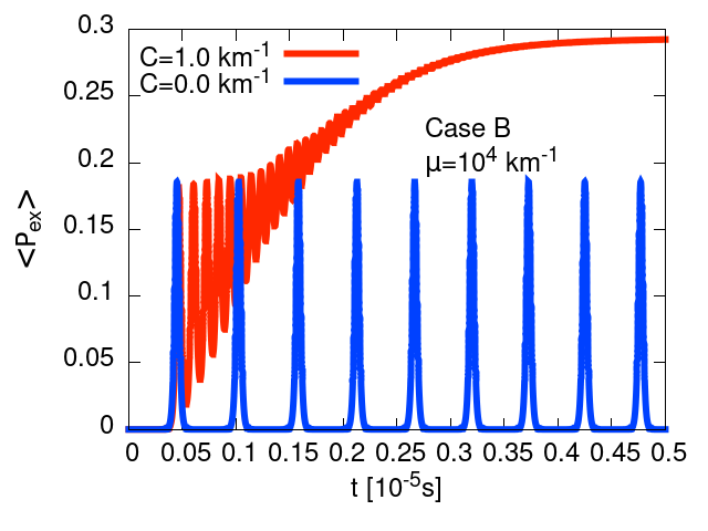
Figure 1: The time evolution of transition probability $\langle P_{ex}\rangle$ with (red) and without (blue) the collision terms.

The dynamics of fast flavor conversions is mainly divided by three epochs such as the linear evolution phase, the limit cycle phase, and the relaxation phase. The fast flavor conversions are enhanced in the limit cycle phase owing to the collision effect. The distribution of neutrinos finally become isotropic in the relaxation phase when the evolution time is comparable with the time scale of the collision term ($ct\sim C^{-1}$), where $c$ is the speed of light. Hereafter we omit $c$ when we convert timescale to length scale.

III.1 Linear evolution phase

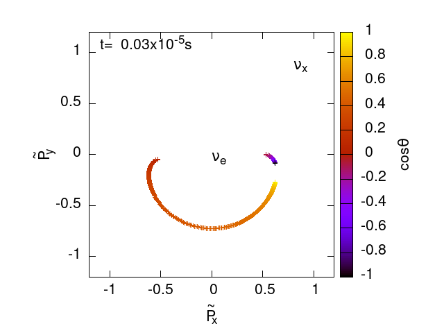
Figure 2: The map of normalized neutrino polarization vector $(\tilde{P}_{x},\tilde{P}_{y})$ in the linear evolution phase ($t=0.03\times 10^{-5}$ s). The normalized polarization vector is defined in Eq. (14).

We call the epoch before reaching the first peak in $\langle P_{ex}\rangle$ linear evolution phase. In this early phase of fast flavor conversions ($t<0.05\times 10^{-5}$ s), the instability of flavor conversions appears near the ELN crossing in the initial distributions of $\nu_{e}$ and $\bar{\nu}_{e}$ ($\cos\theta\sim 0.5$). As shown in Fig. 1, collision effects are negligible in the linear evolution phase because of the large time scale of the collision terms ($t\ll C^{-1}$), so that flavor conversions without and with collision terms are almost equivalent. Here, we use time snapshots of neutrino polarization vectors with $C=1\,\mathrm{km}^{-1}$ at $t=0.03\times 10^{-5}$ s to study behaviors of fast flavor conversions during the linear phase.

Fig. 2 shows a map of normalized neutrino polarization vectors on the $\tilde{P}_{x}-\tilde{P}_{y}$ plane at $t=0.03\times 10^{-5}$ s. In this figure, for the convenience to see a polarization vector in the case of a small transition probability, the polarization vector is normalized as

$$\begin{split}\tilde{P}_{x}&=\left(1+\frac{\log_{10}P_{R}/|P|}{15}\right)\cos(P_{\phi}),\\ \tilde{P}_{y}&=\left(1+\frac{\log_{10}P_{R}/|P|}{15}\right)\sin(P_{\phi}),\end{split}$$ (14)

where $P_{R}=\sqrt{P_{x}^{2}+P_{y}^{2}}$ and $P_{\phi}=\tan^{-1}(P_{y}/P_{x})$ (in this paper, inverse tangent is calculated by atan2 function in C++). At first, all neutrino polarization vectors lie in the $z-$axis ($(0,0)$ in Fig. 2). As the calculation time has passed, the polarization vector begins a spiral motion around the $z-$axis increasing the value of $P_{R}$.

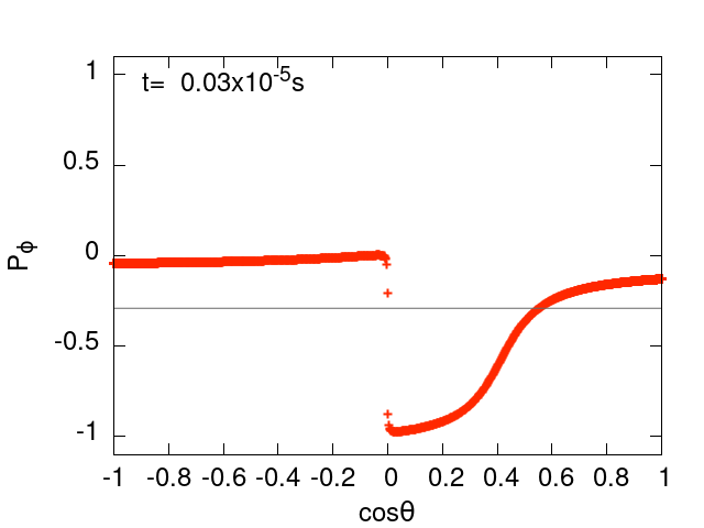
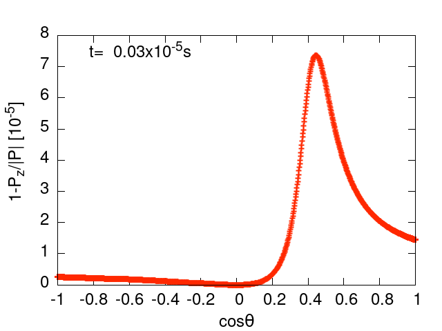
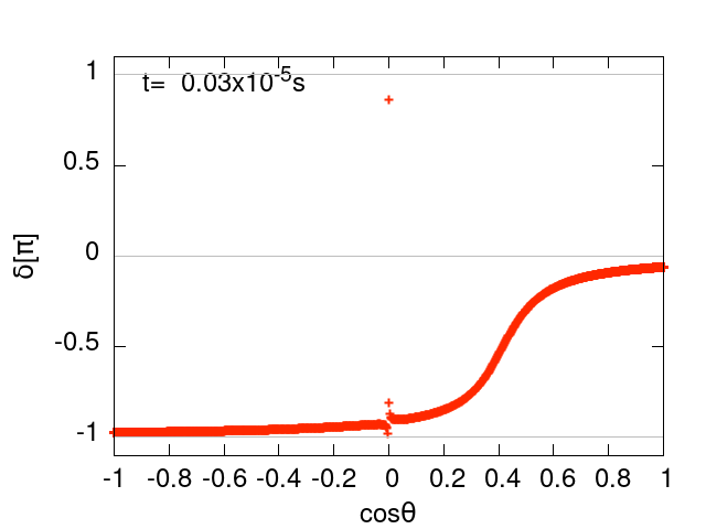
Figure 3: Polarization vector at $t=0.03\times 10^{-5}$ s. Top: The angular distribution of the phase $P_{\phi}=\tan^{-1}(P_{y}/P_{x})$. The gray line is the phase of averaged polarization vector, $\langle P\rangle_{\phi}=\tan^{-1}(\langle P_{y}\rangle/\langle P_{x}\rangle)$. Middle: The angular distribution of $1-P_{z}/|P|$ in the unit of $10^{-5}$. Bottom: The angular distribution of the phase difference $\delta$. The definition of the $\delta$ is given in Eq. (15). The gray lines indicate $1,0,-1$ $[\pi]$.

The dynamics of the polarization can be understood in the cylindrical coordinate ($R$, $\phi$, $z$) as follows. First, we need to define and explain some variables. The quantity $P_{\phi}$ represents a phase of polarization vector on the $\tilde{P}_{x}$-$\tilde{P}_{y}$ plane. In negative value of $\cos\theta$, the motions of polarization vectors synchronize with each other, which results in the same value of $P_{\phi}$ in the top panel of Fig. 3. On the other hand, the phase $P_{\phi}$ is distributed broadly in the case of $\cos\theta>0$. The phase of $\cos\theta>0.6$ is close to that of $\cos\theta<0$. The $P_{\phi}$ becomes opposite phase in $0<\cos\theta<0.2$. The value of $P_{R}$ becomes small around $\cos\theta\sim 0$, so that $\theta=\pi/2$ can be regarded as a singular point for $P_{\phi}$. We discuss the reason why the $P_{R}$ is small around $\cos\theta=0$ in Sec.III.3. The $z$-component of the neutrino polarization vector is related to the transition probability. According to Eq. (13), the transition probability increases as the value of $P_{z}$ decreases. The middle panel of Fig. 3 shows the distribution of $1-P_{z}/|P|$ at $t=0.03\times 10^{-5}$ s. The flavor conversions do not proceed in $\cos\theta<0.2$. However, the flavor conversions become prominent in $\cos\theta\sim 0.4$ that is close to the angle of the ELN crossing ($\cos\theta\sim 0.5$) in the initial distributions. Here, we define the phase difference between $\mathbf{P}$ and the polarization vector of neutrino Hamiltonian $\mathbf{H}$ on the $x$-$y$ plane,

$$\begin{split}H_{R}&=\sqrt{H_{x}^{2}+H_{y}^{2}},\\ \delta&=P_{\phi}-H_{\phi},\end{split}$$ (15)

where $\mathbf{H}=\omega\mathbf{B}+\mu^{\prime}\mathbf{D_{0}}-\mu^{\prime}\cos\theta\mathbf{D_{1}}$ is the polarization vector of neutrino Hamiltonian and $H_{\phi}=\tan^{-1}(H_{y}/H_{x})$ is the phase of $\mathbf{H}$ on the $x$-$y$ plane.The bottom panel of Fig. 3 shows the phase difference $\delta$ in Eq. (15) at $t=0.03\times 10^{-5}$ s. The neutrino polarization vectors are almost antiparallel to the Hamiltonian vector in $\cos\theta<0.2$ because of $\cos\delta\sim-1$. The polarization vector of the neutrino Hamiltonian on the $x$-$y$ plane can be written as Eqs. (45) and (46). Since $H_{x}$ and $H_{y}$ are proportional to $\cos\theta$, $|H_{\phi}(\cos\theta\to+0)-H_{\phi}(\cos\theta\to-0)|\sim\pi$ is satisfied. Therefore, from Eq. (15), the jump ,$|P_{\phi}(\cos\theta\to+0)-P_{\phi}(\cos\theta\to-0)|\sim\pi$ appears around $\cos\theta=0$ as shown in the top panel of Fig. 3.

The evolution of $P_{z}$ is related to the phase difference $\delta$. In the linear evolution phase, the contribution of the collision term is negligible, so that the time evolution of $P_{z}$ is derived from Eq. (9),

$$\frac{\mathrm{d}}{\mathrm{d}t}P_{z}\sim H_{x}P_{y}-H_{y}P_{x}=H_{R}P_{R}\sin\delta.$$ (16)

The value of $\sin\delta$ in Eq. (16) is negligible when the direction of $\mathbf{P_{R}}=(P_{x},P_{y})$ is parallel ($\delta=0$) or antiparallel ($\delta=\pm\pi$) to that of $\mathbf{H_{R}}=(H_{x},H_{y})$ on the $x$-$y$ plane. At $t=0.03\times 10^{-5}$ s, the value of $|\sin\delta|$ is no longer negligible in $\cos\theta>0.2$ and becomes maximum in $\cos\theta\sim 0.4$ (see the bottom panel of Fig. 3), so that fast flavor conversions proceed prominently in $\cos\theta\sim 0.4$ as shown in the middle panel of Fig. 3.

Several studies connect the dynamics of neutrino oscillation with the synchronization phenomena [90, 91, 92]. The evolution of the phase of polarization vector can be interpreted in the framework of the Kuramoto model [93], i.e.,

$$\frac{{\rm d}\phi_{i}}{{\rm d}t}=\omega_{i}+\frac{K}{N}\sum_{j=1}^{N}\sin(\phi_{j}-\phi_{i}),$$ (17)

where $\phi_{i}$ is the phase of $i$-th oscillator, which rotates with the frequency, $\omega_{i}$. The total number of oscillators is $N$ and $K$ is the coupling constant. Sufficiently high $K$ makes synchronization, i.e., all $\phi_{i}$ rotates with the same frequency irrespective to the original $\omega_{i}$. In the context of neutrino oscillation, this is a trivial equilibrium and no flavor conversions happen. The flavor conversion is expected when K becomes slightly lower, and the perfect synchronization is broken [91]. Note that, Refs. [94, 95] consider a more complicated functions, which resemble our setup.

In our case, the strong coupling constant, $\mu$, synchronize the phase: the polarization vector at $\cos\theta>0.6$ and $\cos\theta<0$ rotates with the same phase (see Fig. 3 top panel). Due to the angular distribution with ELN crossing, that at $0<\cos\theta<0.2$ rotates with a different phase but the shape of the $\delta$ is kept in the linear phase, and this part is also synchronized to the average frequency. As a result of the synchronization, $\delta$ is kept to $-\pi/2$ at $\cos\theta\sim 0.4$, and it plays an essential role in the flavor conversion. The profile of $\delta$ in Fig. 3 is clearly explained by the condition of the synchronization, see Appendix A for the details.

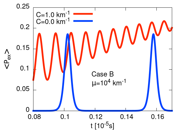
Figure 4: Enlarge view of Fig. 1 in the limit cycle phase.

III.2 Limit cycle phase

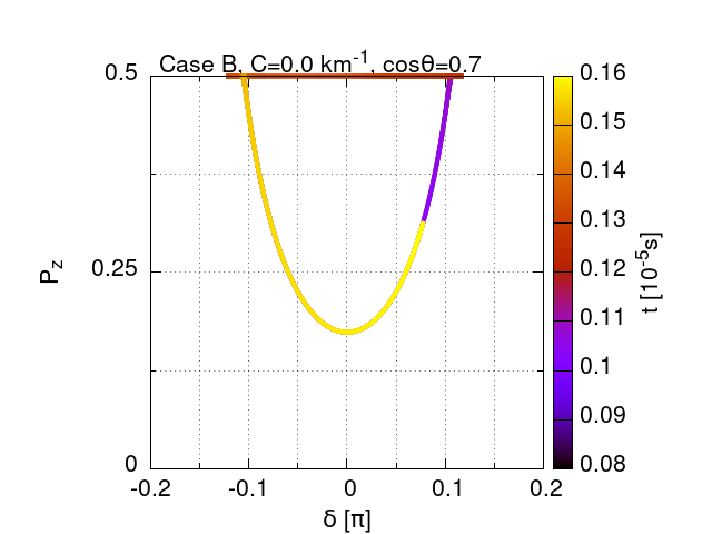
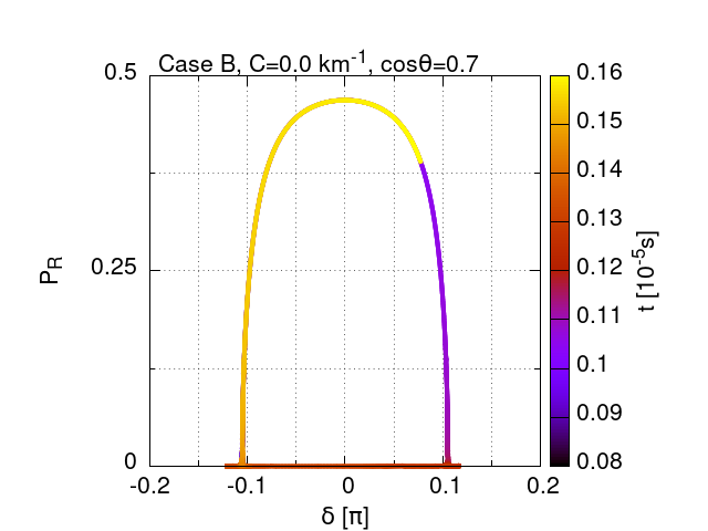
Figure 5: Top: The time evolution of neutrino polarization vector ($\cos\theta=0.7$) on the $\delta$-$P_{z}$ plane from $0.08\times 10^{-5}$ s to $0.16\times 10^{-5}$ s. Here, we set $C=0\,\mathrm{km}^{-1}$. At $t=0.08\times 10^{-5}$ s, $\delta$ is close to $-0.1\pi$. The polarization vector moves counterclockwise along the track. Bottom: The time evolution of polarization vector on the $\delta$-$P_{R}$ plane. The polarization vector moves clockwise along the track.

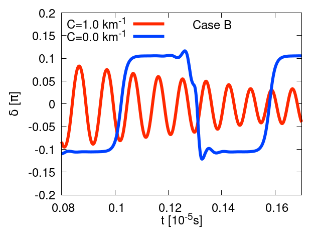
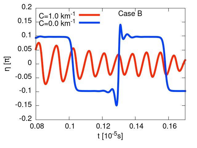
Figure 6: Top: The time evolution of $\delta$ at $\cos\theta=0.7$ in the limit cycle phase. Bottom: The time evolution of $\eta=P_{\phi}-\langle P\rangle_{\phi}$ at $\cos\theta=0.7$ in the limit cycle phase. The blue (red) line shows the case of $C=0\,\mathrm{km}^{-1}$ ($C=1\,\mathrm{km}^{-1}$).

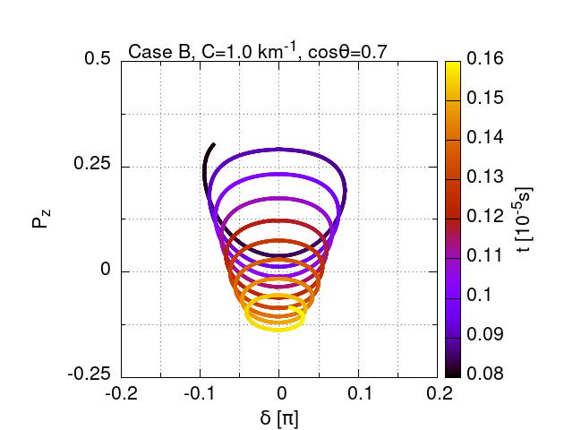
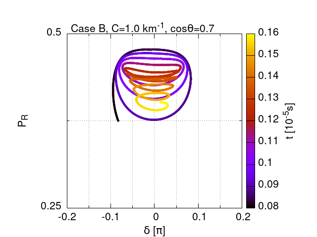
Figure 7: Same to Fig. 5 but here, we consider the collision term ($C=1\,\mathrm{km}^{-1}$).

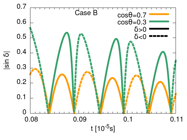
Figure 8: The time evolution of $|\sin\delta|$ at $\cos\theta=0.7$ (orange) and $\cos\theta=0.3$ (green). For positive and negative $\delta$, solid and dashed curve are used, respectively.

Here, we define the limit cycle phase as the period from the linear evolution phase until $\langle P_{ex}\rangle$ settles down to its equilibrium value. Fig. 4 shows an enlarge view of Fig. 1 focusing on the flavor conversions in the limit cycle phase. In the case without collision terms (blue curve), flavor conversions become periodic. On the other hand, in the case with collision term, the amplitude of the flavor conversion becomes gradually smaller and the transition probability is enhanced by collision effect (red curve). In the limit cycle phase, the collision effect is no longer negligible in flavor conversions. We study the collision effect on the motion of neutrino polarization vectors in the limit cycle phase. The equation of motion of $\mathbf{P}$ in Eq. (9) is decomposed by

$$\frac{\mathrm{d}}{\mathrm{d}t}P_{z} =\;\;H_{R}P_{R}\sin\delta-C\left(P_{z}-\langle P_{z}\rangle\right),$$ (18)

$$\frac{\mathrm{d}}{\mathrm{d}t}P_{R} =-H_{R}P_{z}\sin\delta-C\left(P_{R}-\langle P\rangle_{R}\cos\eta\right),$$ (19)

$$P_{R}\frac{{\rm d}P_{\phi}}{{\rm d}t} =-H_{R}P_{z}\cos\delta-C\langle P\rangle_{R}\sin\eta+P_{R}H_{z}$$ (20)

where $H_{R}$ and $\delta$ are given in Eq. (15), and $\eta=P_{\phi}-\langle P\rangle_{\phi}$. Note that we first calculate average polarization $\langle P_{x}\rangle$ and $\langle P_{y}\rangle$, and then obtain $\langle P\rangle_{R}=\sqrt{\langle P_{x}\rangle^{2}+\langle P_{y}\rangle^{2}}$ and $\langle P\rangle_{\phi}=\tan^{-1}\left(\langle P_{y}\rangle/\langle P_{x}\rangle\right)$. In general, $\langle P\rangle_{R}\neq\langle P_{R}\rangle$ and $\langle P\rangle_{\phi}\neq\langle P_{\phi}\rangle$, where the right hand sides are the average of $P_{R}$ and $P_{\phi}$, respectively.

Fig. 5 shows the time evolution of $P_{z}$ and $P_{R}$ at $\cos\theta=0.7$ without the collision ($C=0\,\mathrm{km}^{-1}$) during $t$ in $0.08\text{--}0.16$ in the unit of $10^{-5}\,\mathrm{s}$, respectively. Without collision terms, the evolution tracks of polarization vectors in Fig. 5 are closed. The blue curve in the top panel of Fig. 6 shows the evolution of $\delta$ without collision effect. At first, the value of $\delta$ is approximately $-0.1\pi$ and almost constant. The value of $\delta$ increases dramatically around $t=0.1\times 10^{-5}$ s. According to the first terms on the right hand sides of Eqs. (18) and (19), the value of $P_{z}$ ($P_{R}$) decreases (increases) when the $\delta$ is negative. In the case of positive $\delta$, the value of $P_{z}$ ($P_{R}$) increases (decreases). The perpendicular component is negligible ($P_{R}\sim 0$) and the $z$-component is constant ($P_{z}\sim 0.5$) at $t=(0.12\text{--}0.14)\times 10^{-5}$ s irrespective of decreasing $\delta$. In such evolution phase, the small $H_{R}$ suppresses the time evolution of $P_{z}$ and $P_{R}$. Therefore, the polarization vector moves counterclockwise (clockwise) in Top panel (Bottom panel) of Fig. 5.

In the case with neutrino scatterings ($C=1\,\mathrm{km}^{-1}$), the evolution track of neutrino polarization vector is no longer a closed orbit but a “limit cycle” on the phase space because of the collision terms in Eqs.(18) and (19). The spiral motion of $P_{z}$ and $P_{R}$ at $\cos\theta=0.7$ is shown in the top and bottom panels of Fig. 7, respectively. The value of $\delta$ is negative at $t=0.08\times 10^{-5}$ s (see the red curve in the top panel of Fig. 6). By the first term on the right hand side of Eq. (18) (Eq. (19)), the value of $P_{z}$ ($P_{R}$) decreases (increases) at first. On the other hand, in more later phase, $\delta$ becomes positive and $P_{z}$ ($P_{R}$) increases (decreases).

The ranges of $P_{z}$ and $P_{R}$ changing in one cycle gradually decrease with each cycle. As shown in the red curve of the top panel of Fig. 6, the oscillation amplitude of $\delta$ is decreasing and converging to zero. In the bottom panel, the evolution of $\eta$ is also shown. Comparing the top and bottom panels, we found $\delta\sim-\eta$. Since the collision tries to align the polarization and decreases $|\eta|=|P_{\phi}-\langle P\rangle_{\phi}|$, $|\delta|\sim|\eta|$ is also expected to become smaller as time passes. After such synchronization between $\mathbf{P_{R}}$ and $\mathbf{H_{R}}$, the first terms on the right hand side of Eqs. (18) and (19) are negligible and the transition probability $\langle P_{ex}\rangle$ no longer changes, which results in the end of the limit cycle phase.

One of the most interesting features of this model is that the mean value of $P_{z}$ becomes smaller as time passes (e.g., top of Fig. 7). Fig. 8 shows $|\sin\delta|$. It is similar to Fig. 6, but we can compare positive $\delta$ and negative $\delta$ easily. In the case of $\cos\theta=0.7$, the averaged $|\sin\delta|$ for negative $\delta$ is larger than that of positive $\delta$ in one cycle. In addition, the period with negative $\delta$ is slightly longer than the positive part. From Eq. (18), this imbalance of positive and negative $\delta$ leads to the gradual decrease of $P_{z}$. Note that this does not happen for all $\theta$. In the case of $\cos\theta=0.3$, on the other hand, the positive part is slightly larger than the positive part. This excess slightly increases the mean $P_{z}$ (see the bottom of Fig. 10).

This imbalance comes from the highly non-linear dynamics of the partially synchronized oscillators, and it is difficult to identify the mechanism to produce that. Here we show a hypothesis of the possible origin, focusing on the impact of the collision term on $\delta=P_{\phi}-H_{\phi}$. Note that other terms may also cause the imbalance. First we extract the impact of the collision term on the phase of the polarization vector: $\left.\frac{{\rm d}P_{\phi}}{{\rm d}t}\right|_{\rm coll}=\frac{{\rm d}P_{\phi}}{{\rm d}t}-\left.\frac{{\rm d}P_{\phi}}{{\rm d}t}\right|_{C=0}$, where $\left.\frac{{\rm d}P_{\phi}}{{\rm d}t}\right|_{C=0}$ is obtained by substituting $C=0$ in Eq. (20). Similarly, we consider the collisional part of $\delta$: $\left.\frac{{\rm d}\delta}{{\rm d}t}\right|_{\rm coll}=\frac{{\rm d}\delta}{{\rm d}t}-\left.\frac{{\rm d}\delta}{{\rm d}t}\right|_{C=0}$ . This term could be well approximated as

$$\left.\frac{{\rm d}\delta}{{\rm d}t}\right|_{\rm coll} =\left.\frac{{\rm d}P_{\phi}}{{\rm d}t}\right|_{\rm coll}-\left.\frac{{\rm d}H_{\phi}}{{\rm d}t}\right|_{\rm coll} \sim-C\left(\frac{\langle P\rangle_{R}}{P_{R}}\right)\sin\eta,$$ (21)

where we ignore the effect of the collision term in $\frac{{\rm d}H_{\phi}}{{\rm d}t}$ following Appendix B, and the collision term in Eq. (20) is extracted.

We demonstrate how the collision term violates the time symmetry using the schematic diagram of Fig. 9. Near $t=0.0945\times 10^{-5}\,{\rm s}$ in Fig. 8, $\delta$ of $\cos\theta=0.7$ changes its sign from negative to positive, i.e., $\frac{{\rm d}\delta}{{\rm d}t}>0$ (point A in the diagram). The collision term would decelerate $\delta$ when $t<0.0945\times 10^{-5}\,{\rm s}$ and $\delta<0$ since the collision term, $\left.\frac{{\rm d}\delta}{{\rm d}t}\right|_{\rm coll}$, is proportional to $-C\sin\eta\sim C\sin\delta<0$ ( here $\eta\sim-\delta$. see Fig. 6). Now $\frac{{\rm d}\delta}{{\rm d}t}$ is positive, and $\left.\frac{{\rm d}\delta}{{\rm d}t}\right|_{\rm coll}$ is negative, then the evolution of $\delta$ would be decelerated by the collision (curve of D to A in the diagram). On the other hand, when $t>0.0945\times 10^{-5}\,{\rm s}$ and $\delta>0$, the collision term accelerate the evolution of $\delta$ since $\frac{{\rm d}\delta}{{\rm d}t}>0$ and $\left.\frac{{\rm d}\delta}{{\rm d}t}\right|_{\rm coll}$ are both positive (Curve A-B in the diagram). These two effects make the duration in negative $\delta$ longer and positive $\delta$ shorter. Caveat that at $t=0.099\times 10^{-5}\,{\rm s}$, the collision term, vise versa, makes the duration in negative $\delta$ shorter and the duration in positive $\delta$ longer. Here $\frac{{\rm d}\delta}{{\rm d}t}<0$, and $\left.\frac{{\rm d}\delta}{{\rm d}t}\right|_{\rm coll}>0$ ($<0$) for positive (negative) $\delta$ in Curve B-C (C-D). We need more careful analysis for quantitative argument, which we keep in a future study as well as the possibility of other origin.

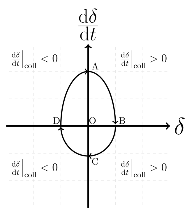
Figure 9: Schematic diagram of the evolution of $\delta$ and $\frac{{\rm d}\delta}{{\rm d}t}$ .

III.3 Relaxation phase

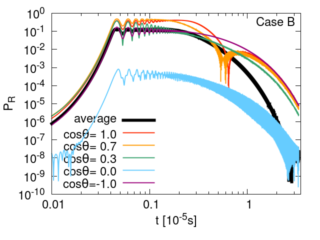
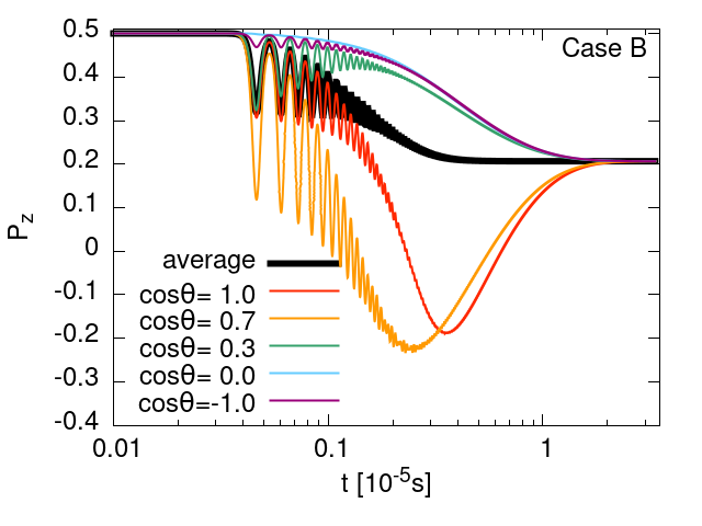
Figure 10: Top: The time evolution of perpendicular component of neutrino polarization vectors at different angles (color curves), $P_{R}$, and that of angle averaged one (black), $\langle P\rangle_{R}$. Bottom: The time evolution of $P_{z}$ at different angles and that of the angle averaged $z$-component $\langle P_{z}\rangle$. The red, orange, green, cyan, and purple curves show the case of $\cos\theta=1,0.7,0.3,0$ and $-1$, respectively.

As implied in Eq. (11), the distributions of neutrinos affected by fast flavor conversions become isotropic in the relaxation phase ($t>C^{-1}=0.33\times 10^{-5}$ s). Up to the limit cycle phase, the fast flavor conversions are enhanced by collision effects and the transition probability $\langle P_{ex}\rangle$ does not change anymore as shown in Fig. 1. In the relaxation phase, the collision terms force all of polarization vectors to face $z$-axis keeping the value of $\langle P_{ex}\rangle$.

The top panel of Fig. 10 shows the time evolution of $P_{R}$ in different angles and that of $\langle P\rangle_{R}$. Owing to the coupling of neutrino-neutrino interactions with neutrino scatterings, the value of $P_{R}$ increases and saturates around $t\sim 0.1\times 10^{-5}$ s. Note that the time of the first peak would depend on the initial perturbation. We impose $P_{R}\sim 10^{-8}$, initially. After the saturation, all of polarization vector starts to be parallel to the $z$-axis and the values of $P_{R}$ are reduced to zero. The perpendicular component of $\cos\theta=0$ (cyan curve) is small and the polarization vector always points near the $z$-axis. From Eqs.(9) and (10), equation of motions of $\mathbf{D_{0}}$ is described by

$$\frac{\mathrm{d}}{\mathrm{d}t}\mathbf{D_{0}}=\omega\left(\langle\mathbf{P}\rangle+\langle\mathbf{\bar{P}}\rangle\right)\times\mathbf{B}.$$ (22)

The above equation of motion indicates that, in the case of a small vacuum frequency ($\omega t\ll 1$), $\mathbf{D_{0}}$ is almost conserved during the flavor conversions and parallel to the $z$-axis. In addition, $\mathbf{B}$ is also directed to the $z$-axis in the case of a small mixing angle ($\theta_{\mathrm{v}}\ll 1$). Then, $\omega\mathbf{B}+\mu^{\prime}\mathbf{D_{0}}$ in Eq. (9) is also parallel to the $z$-axis, so that the $P_{R}$ is almost negligible at $\cos\theta=0$. The evolution of $P_{z}$ in different angles and that of $\langle P_{z}\rangle$ are shown in the bottom panel of Fig. 10. The fast flavor conversions increase the transition probability and induce different values of $P_{z}$ depending on the scattering angle $\theta$ until the end of the limit cycle $t\sim C^{-1}=0.33\times 10^{-5}$ s. The flavor conversions in the limit cycle phase are especially enhanced at $\cos\theta=0.7$ (orange curve) and $\cos\theta=1$ (red curve) in the bottom panel of Fig. 10. Such enhancement of flavor conversions in forward scattered neutrinos is also confirmed in the middle panel of Fig.11. However, after the limit cycle, the values of $P_{z}$ in different angles (color curves) converge on the value of $\langle P_{z}\rangle$ (black curve). Then, the fast flavor conversions of neutrinos have finished when $P_{z}=\langle P_{z}\rangle$ is satisfied in all of the scattering angles. Such behaviors of $P_{z}$ can be understood by the equation of motion of $P_{z}$ in the relaxation phase. Eq.(13) shows that the $\langle P_{z}\rangle$ is related to the transition probability as $\langle P_{ex}\rangle=0.5-\langle P_{z}\rangle$ in our numerical setup. As discussed in Sec. III.2, the time evolution of $\langle P_{ex}\rangle$ reaches an equilibrium in the limit cycle phase owing to the synchronization between polarization vectors of neutrino density matrix and that of Hamiltonian ($\mathbf{P_{R}}\parallel\mathbf{H_{R}}$). Therefore, the value of $\delta$ is negligible and the value of $\langle P_{z}\rangle$ becomes constant before the relaxation phase. Then, the equation of motion of $P_{z}$ in the relaxation phase is derived from Eq. (18),

$$\frac{\mathrm{d}}{\mathrm{d}t}P_{z}\sim-C\left(P_{z}-\langle P_{z}\rangle\right),$$ (23)

which explains the relaxation of $P_{z}$ to $\langle P_{z}\rangle$ in all scattering angles at $t>C^{-1}=0.33\times 10^{-5}$ s as shown in the bottom panel of Fig.10. Here, we discuss the relaxation of polarization vectors in neutrino sector, but the case of antineutrinos are similar. In the case of antineutrinos, the polarization vector $\mathbf{\bar{P}}$ is relaxed to $(0,0,\langle\bar{P}\rangle)$ irrespective of the scattering angle $\theta$.

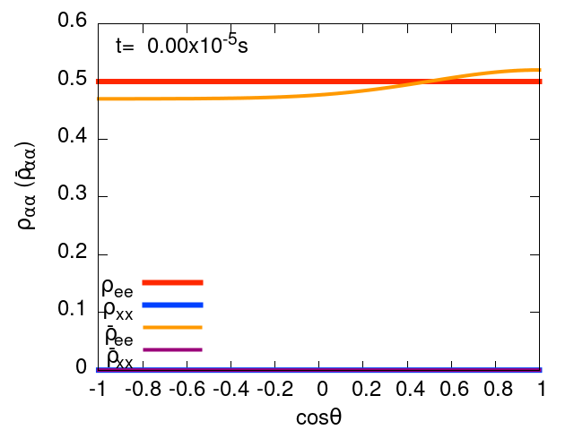
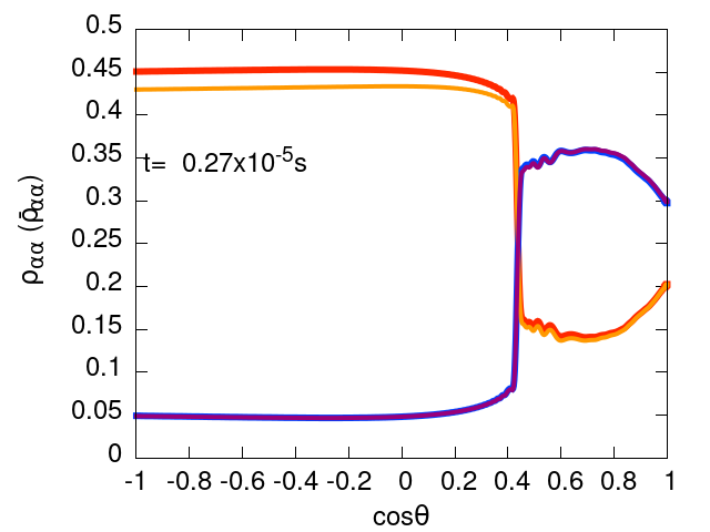
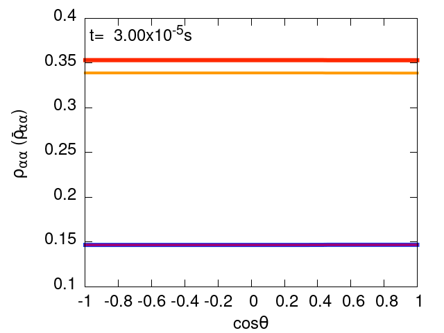
Figure 11: Time snapshots of neutrino spectra. The initial ($t=0$ s), after limit cycle ($t=0.27\times 10^{-5}$ s), after the relaxation ($t=3.00\times 10^{-5}$ s) snapshots are taken, respectively. The distribution of $\rho_{ee}$, $\rho_{xx}$, $\bar{\rho}_{ee}$, and $\bar{\rho}_{xx}$ correspond to red, blue, orange, and purple curves, respectively.

The angular distributions of neutrinos after fast flavor conversions are shown in Fig. 11 bottom panel. As implied in Eq. (11), the angular dependence disappears in the distribution of neutrinos. The density matrices of neutrinos (antineutrinos) become diagonal because of the negligible $P_{R}$($\bar{P}_{R}$) and the finite $P_{z}$($\bar{P}_{z}$). The middle panel is taken at $t=0.27\times 10^{-5}$ s. Up to the limit cycle, the values of $\rho_{ee}$ and $\bar{\rho}_{ee}$ depend on the scattering angle [73]. It looks similar to the stationary solution without collision [78]. However, such angular dependence disappear during the relaxation phase and the neutrino distribution becomes isotropic because of the collision effect. In Fig. 11 bottom panel, the value of $\rho_{xx}$ (blue curve) is equal to that of $\bar{\rho}_{xx}$ (purple curve). Such correspondence can be explained by a conservation law below

$$\mathbf{B}\cdot\mathbf{D_{0}}=\mathrm{const.}\,.$$ (24)

The above equation is derived from Eq. (22). In the case of small vacuum mixing angle, $\langle P_{z}\rangle-\langle\bar{P}_{z}\rangle$ is almost conserved according to Eq. (24). Furthermore the $\langle\mathrm{Tr}\rho\rangle$ and $\langle\mathrm{Tr}\bar{\rho}\rangle$ are time-independent quantities. Therefore, we can show that $\langle\rho_{xx}\rangle$ is almost equal to $\langle\bar{\rho}_{xx}\rangle$ at any time:

$$\begin{split}\langle\rho_{xx}\rangle-\langle\bar{\rho}_{xx}\rangle&=\frac{\langle\mathrm{Tr}\rho\rangle}{2}-\frac{\langle\mathrm{Tr}\bar{\rho}\rangle}{2}-\frac{\langle P_{z}\rangle}{2}+\frac{\langle\bar{P}_{z}\rangle}{2}\\ &\sim\left(\langle\rho_{xx}\rangle-\langle\bar{\rho}_{xx}\rangle\right)(t=0)\\ &=0.\end{split}$$ (25)

After the relaxation phase, neutrino distribution becomes isotropic, so that $\rho_{xx}\sim\bar{\rho}_{xx}$ is satisfied in the end of the calculation as shown in Fig. 11.

Note that the appearance of the relaxation phase depends on the situation. The ELN crossing, considered here, typically appears above the neutrino sphere [67], and it means the opacity is less than one, i.e., $t<C^{-1}$. On the other hand, the ELN crossing in proto-neutron stars, opacity is larger than one, and the relaxation phase should be considered. In any case, the discussion here would be helpful to understand the role of the collision term.

III.4 Dependence of neutrino scattering terms

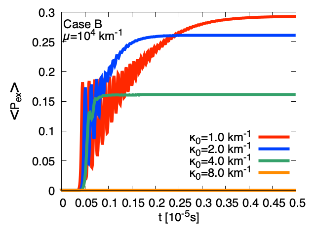
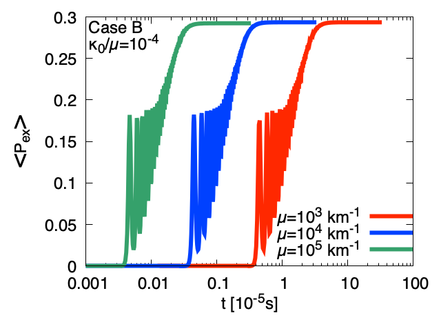
Figure 12: Top: The time evolution of Eq.(12) with NC collision terms in Eqs. (26) and (27) with different values of $\kappa_{0}$. Bottom: The results with different values of $\mu$ with $\kappa_{0}/\mu=10^{-4}$. Here, we finished the calculations of $\mu=10^{n}\,\mathrm{km}^{-1}$ at $t=3.3\times 10^{-1-n}$ s ($n=3,4,5$).

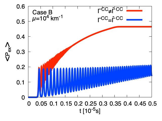
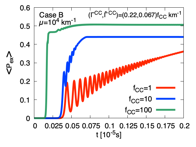
Figure 13: Top: The time evolution of Eq.(12) with CC collision terms in Eqs. (32) and (37). The red curve shows the result of asymmetric case, i.e., $\Gamma^{\rm CC}=0.22\,\mathrm{km}^{-1}$ and $\bar{\Gamma}^{\rm CC}=0.067\,\mathrm{km}^{-1}$. The blue curve shows the result of the symmetric case, $\Gamma^{\rm CC}=\bar{\Gamma}^{\rm CC}=0.22\,\mathrm{km}^{-1}$. Bottom: The results with different strengths of the CC collision terms, $\Gamma^{\rm CC}=0.22f_{\rm CC}\,\mathrm{km}^{-1}$ and $\bar{\Gamma}^{\rm CC}=0.067f_{\rm CC}\,\mathrm{km}^{-1}$, where $f_{\rm CC}=1,10,$ and $100$.

In the previous section, we confirm that the collision terms of Eqs. (5) and (6) enhance fast neutrino flavor conversions and make neutrino angular distributions isotropic. In this section, we calculate angle averaged transition probabilities by using collision terms of neutrino scatterings in Refs. [76, 82]. We use the same numerical setup as that of the previous section except for the collision term.

First, we consider the collision terms of neutrino scatterings in neutral-current (NC) reactions. For the updated NC reaction, we employ the elastic neutrino-nucleon collision in Ref. [76],

$$C^{\mathrm{NC}}[\rho]= -\kappa_{0}\rho(\cos\theta)$$

$$+\frac{1}{2}\int^{1}_{-1}\mathrm{d}\cos\theta^{\prime}\left(\kappa_{0}-\frac{\kappa_{1}}{3}\cos\theta\cos\theta^{\prime}\right)\rho(\cos\theta^{\prime}),$$ (26)

$$\bar{C}^{\mathrm{NC}}[\bar{\rho}]= -\kappa_{0}\bar{\rho}(\cos\theta)$$

$$+\frac{1}{2}\int^{1}_{-1}\mathrm{d}\cos\theta^{\prime}\left(\kappa_{0}-\frac{\kappa_{1}}{3}\cos\theta\cos\theta^{\prime}\right)\bar{\rho}(\cos\theta^{\prime}),$$ (27)

where we fix $\kappa_{1}/\kappa_{0}=0.5$ as in Ref.[76]. The gain terms in the above NC collisions depend on the neutrino scattering angle $\theta$. The collision terms in Eqs. (5) and (6) are reproduced, when $\kappa_{1}=0\,\mathrm{km}^{-1}$ and $\kappa_{0}=C$.

The top panel of Fig. 12 shows the evolution of the transition probability $\langle P_{ex}\rangle$ in Eq. (12) with different values of $\kappa_{0}$. In the case of $\kappa_{0}=1\,\mathrm{km}^{-1}$ (red curve), the flavor conversion is well enhanced by the collision effect and the result is almost identical to that of $C=1\,\mathrm{km}^{-1}$ in Fig. 1. This correspondence suggests the small contribution of $\kappa_{1}$ to the NC scattering. As shown in the blue, green, and orange curves in Fig. 12, the flavor conversions are more suppressed in the large value of $\kappa_{0}$. Any flavor conversion does not appear in $\kappa_{0}\geq 8\,\mathrm{km}^{-1}$, where all of the polarization vectors are directed to the $z$-axis by strong collision terms so that the instability for fast flavor conversions does not grow up sufficiently. Nothing is happening in the neutrino sector, but the distribution of electron antineutrino becomes isotropic following the classical Boltzmann equation without neutrino oscillations. Such damping effect of a large $\kappa_{0}$ is consistent with the result of Ref. [76].

The bottom panel of Fig. 12 shows the results with different values of $\mu$ while maintaining the ratio, $\kappa_{0}/\mu=10^{-4}$. The transition probabilities scale to $\mu^{-1}$ and the flavor conversion is raised even with the large collision parameter, $\kappa_{0}=10\,\mathrm{km}^{-1}$ (green curve). Therefore, the collision effect can be characterized by the ratio, $\kappa_{0}/\mu$. It seems that a small collision term, $\kappa_{0}\leq\tau^{-1}_{\rm{osc}}\propto\mu$ is required to enhance the flavor conversions, where $\tau_{\rm{osc}}$ is a characteristic oscillation time proportional to $\mu^{-1}$.

Next, we consider charged-current (CC) reactions. For the CC scatterings, we study the effect of neutrino electron scatterings following the collision term in Ref. [82],

$$C^{\mathrm{\rm CC}}[\rho]= -\Gamma^{\rm CC}\left(\begin{array}[]{cc}\rho_{ee}&\frac{\rho_{ex}}{2}\\ \frac{\rho_{xe}}{2}&0\end{array}\right)+\Gamma^{\rm CC}\left(\begin{array}[]{cc}\langle\rho_{ee}\rangle&0\\ 0&0\end{array}\right),$$ (32)

$$\bar{C}^{\mathrm{\rm CC}}[\bar{\rho}]= -\bar{\Gamma}^{\rm CC}\left(\begin{array}[]{cc}\bar{\rho}_{ee}&\frac{\bar{\rho}_{ex}}{2}\\ \frac{\bar{\rho}_{xe}}{2}&0\end{array}\right)+\bar{\Gamma}^{\rm CC}\left(\begin{array}[]{cc}\langle\bar{\rho}_{ee}\rangle&0\\ 0&0\end{array}\right),$$ (37)

where $\Gamma^{\rm CC}=1/\lambda_{\nu_{e}e}$ and $\bar{\Gamma}^{\rm CC}=1/\lambda_{\bar{\nu}_{e}e}$ are calculated from the rates of the electron scatterings (see Eq. ($11$) in Ref. [82]). The red curve in the top panel of Fig. 13 shows the transition probability $\langle P_{ex}\rangle$ in Eq. (12) for the typical values at a post-bounce near the proto-neutron star, $\Gamma^{\rm CC}=0.22\,\mathrm{km}^{-1}$ and $\bar{\Gamma}^{\rm CC}=0.067\,\mathrm{km}^{-1}$ for $E=50$ MeV neutrinos. The transition probability increases due to the collision effect as in Fig. 1. The equilibrium value of transition probability is larger than that of the NC scattering because of the large asymmetry, $\Gamma^{\rm CC}\neq\bar{\Gamma}^{\rm CC}$. On the other hand, the flavor conversion does not equilibrate immediately for the symmetric collision parameter, $\Gamma^{\rm CC}=\bar{\Gamma}^{\rm CC}=0.22\,\mathrm{km}^{-1}$, as shown in the blue curve in the top panel of Fig. 13. Such property between $\Gamma^{\rm CC}$ and $\bar{\Gamma}^{\rm CC}$ is also reported in Ref. [82]. Our results clarify the role of the asymmetry on the CC scatterings.

In the symmetric case, when $\Gamma^{\rm CC}=\bar{\Gamma}^{\rm CC}\geq 8\,\mathrm{km}^{-1}$, the flavor conversions are strongly suppressed, as in the NC scattering. On the other hand, as shown in the bottom panel of Fig. 13, the flavor conversions in the asymmetric case are not suppressed even in the large collision terms ($f_{\rm CC}=10,100$). In the asymmetric case, collision terms associated with $\Gamma^{\rm CC}-\bar{\Gamma}^{\rm CC}$ can couple the time evolution of $\mathbf{D}_{n}=~{}\langle(\mathbf{P}-\mathbf{\bar{P}})\cos^{n}\theta\rangle$ and that of $\mathbf{S}_{m}=~{}\langle(\mathbf{P}+\mathbf{\bar{P}})\cos^{m}\theta\rangle$ to each other [82]. Such coupling may make a qualitative difference between the collision effect in the symmetric case and that of the asymmetric case. The asymmetry of the collision rate is quite possible in explosive astrophysical sites. Here we focus on monochromatic energy neutrinos, but the asymmetry of the collision rate can be increased by considering the energy dependence of neutrinos.

IV Conclusions

We calculate fast flavor conversions with collision effects of neutrino scatterings and analyze behaviors of the flavor conversions based on the dynamics of neutrino polarization vectors in cylindrical coordinate where we can easily access the information of the phase of rotation.

We find that the the collision terms in Ref. [73] induce enhancement of flavor conversions and isotropization of neutrino distributions. In the linear phase, the instability of fast flavor conversions grows up around the ELN crossing where the phase difference $\delta$ takes an intermediate value in the range between $0$ and $-\pi$. In the limit cycle phase, the evolution track of neutrino polarization vector without collision effects is closed, and flavor conversions show a periodic trend. On the other hand, with the collision terms, the evolution track of the neutrino polarization vector is no longer closed because of the decrease of $|\delta|$ in every cycle. The collision term breaks the symmetry between positive and negative $\delta$, and the induced imbalance enhances the total transition probability. After the synchronization of neutrino polarization vectors, the value of $\delta$ finally converges to zero. At the end of the limit cycle, the evolution of $\langle P_{ex}\rangle$ settles down to equilibrium, and the distributions of neutrinos are dependent on the neutrino scattering angle. Such properties are well consistent with the results in Ref. [73]. However, in the relaxation phase, all of the neutrino polarization vectors align with the $z$-axis keeping the value of $\langle P_{ex}\rangle$. The distributions of neutrinos finally become isotropic after the relaxation phase.

Furthermore, we calculate the effect of collision terms used in previous studies, which helps unify presently disparate effects of collisional instability. For the NC scattering, the flavor conversions are enhanced in the small collision term. On the other hand, the large collision term prevents flavor conversions. Our results suggest that the collision effect is characterized by the ratio of the parameters between collision terms and neutrino-neutrino interactions. For the CC scattering, the transition probability is significantly raised up in a large asymmetry between neutrino and antineutrino collision rates. In the case of the asymmetric CC collision terms, the flavor conversions are not suppressed even in large collision parameters.

Here, we remark on the uncertainties of our works. The calculation results of fast flavor conversions are very sensitive to the numerical setup. The flavor conversions without collisions are highly periodic in our calculation assuming the spatial homogeneity and ignoring the azimuthal angle dependence. In some case, even without the collision term, fast flavor conversions can decay and reach a stationary solution [78]. It has been shown that the flavor conversions become more chaotic and non-periodic in spatial inhomogeneous system [75, 77]. In addition, the periodic structure of flavor conversions is broken in the calculation with the azimuthal angle dependence [81, 83]. The significant enhancement of flavor conversions due to the collision effect may be obscured, when the assumption in our calculation is relaxed. Our simplified numerical setup should be updated in order to study the collision effect precisely in more realistic environment. Here, we focus on behaviors of fast flavor conversions of two flavor neutrinos for simplicity, but three flavors of neutrinos are required to predict the reliable neutrino signal in explosive astrophysical sites.

Appendix A Synchronization in linear phase

Here we focus on the phase $\delta$ seen in Fig. 3 in detail. The time derivative is written as

$$\frac{{\rm d}\delta}{{\rm d}t}=H_{z}-\frac{{\rm d}H_{\phi}}{{\rm d}t}-\left(\frac{P_{z}}{P_{R}}\right)H_{R}\cos\delta,$$ (38)

where we ignore the collision term, which is not important in the linear phase. When the synchronization condition,

$$\frac{{\rm d}\delta}{{\rm d}t}=0,$$ (39)

is satisfied, the profile of $\delta$ is derived from Eq. (38),

$$\delta\sim\cos^{-1}\left[\frac{H_{z}-\frac{\mathrm{d}{H}_{\phi}}{\mathrm{d}t}}{H_{R}}\left(\frac{P_{R}}{P_{z}}\right)\right].$$ (40)

The value of $\delta$ indicates the susceptibility to the flavor conversion. From the above equation, we obtain the following condition for $\delta=\pm\frac{\pi}{2}$,

$$H_{z}=\frac{\mathrm{d}{H}_{\phi}}{\mathrm{d}t}.$$ (41)

At this point, the significant flavor conversion is expected from Eq. (16).

We confirmed that the synchronization condition of Eq. (39) holds in the present calculation. In fact, Eq. (40) reproduces well the result of $\delta$ in Fig. 3. The value of $\delta$ is negative because the synchronization is stable, $\frac{\partial}{\partial\delta}(\frac{{\rm d}\delta}{{\rm d}t})<0$. In addition, Eq. (41) is satisfied at $\cos\theta\sim 0.4$ in the linear phase. In terms of synchronizing phenomena, we can predict the angle $\theta$ at which flavor conversions will occur.

The analysis above is based on the textbook of synchronization phenomena (Section 4.10 of Ref. [96], which is written in Japanese), many types of phase equation are solved in the book. In the case of the coupling two oscillators,

$$\frac{{\rm d}\phi_{1}}{{\rm d}t} =\omega_{1}+\Gamma(\phi_{1}-\phi_{2}),$$ (42)

$$\frac{{\rm d}\phi_{2}}{{\rm d}t} =\omega_{2}+\Gamma(\phi_{2}-\phi_{1}),$$ (43)

it is useful to take the phase difference $\psi=\phi_{1}-\phi_{2}$,

$$\frac{{\rm d}\psi}{{\rm d}t} =\Gamma_{a}(\psi),$$ (44)

where $\Gamma_{a}$ contains the asymmetric part of $\Gamma$ and the contribution of $\omega_{1}-\omega_{2}$. The condition for the synchronization is given by $\Gamma_{a}=0$ and $\frac{{\partial}\Gamma_{a}}{\partial\psi}<0$. The second condition ensures the stability for small perturbation on $\psi$, i.e., $\frac{{\rm d}\psi}{{\rm d}t}$ is negative (positive) for positive (negative) perturbations. This general argument is also applicable to our system as $\phi_{1}=P_{\phi}$, $\phi_{2}=H_{\phi}$ and $\psi=\delta$.

Appendix B The derivation of Eq. (21)

As discussed in Sec. III.3, both $\mathbf{D_{0}}$ and $\mathbf{B}$ are almost parallel to the $z$-axis when vacuum frequency and the mixing angle are small. In such a case, the polarization vector of neutrino Hamiltonian on the $x$-$y$ plane is described by

$$H_{x} \sim-\mu^{\prime}\cos\theta D_{1x},$$ (45)

$$H_{y} \sim-\mu^{\prime}\cos\theta D_{1y},$$ (46)

where $D_{1x}$ and $D_{1y}$ are $x$ and $y$ components of $\mathbf{D_{1}}$ in Eq. (10). Then, the equation of motion of $H_{i}(i=x,y)$ is written as

$$\frac{\mathrm{d}H_{i}}{\mathrm{d}t}\sim\left.\frac{\mathrm{d}H_{i}}{\mathrm{d}t}\right|_{C=0}-CH_{i},$$ (47)

where the first term on the right hand side of Eq. (47) does not include the collision parameter $C$ explicitly. From Eq. (47), the time derivative of the phase ${H}_{\phi}$ is given by

$$\frac{\mathrm{d}H_{\phi}}{\mathrm{d}t}=-\frac{1}{H_{R}^{2}}\left(H_{y}\frac{\mathrm{d}H_{x}}{\mathrm{d}t}-H_{x}\frac{\mathrm{d}H_{y}}{\mathrm{d}t}\right)\sim\left.\frac{\mathrm{d}{H}_{\phi}}{\mathrm{d}t}\right|_{C=0}.$$ (48)

Finally, Eq. (21) is derived from Eqs. (20) and (48).

References

- Vitagliano et al. [2020] E. Vitagliano, I. Tamborra, and G. Raffelt, Grand Unified Neutrino Spectrum at Earth: Sources and Spectral Components, Rev. Mod. Phys. 92, 45006 (2020), arXiv:1910.11878 [astro-ph.HE] .
- Horiuchi and Kneller [2018] S. Horiuchi and J. P. Kneller, What can be learned from a future supernova neutrino detection?, Journal of Physics G: Nuclear and Particle Physics 45, 043002 (2018).
- Janka [2017] H.-T. Janka, Neutrino Emission from Supernovae, in Handbook of Supernovae, 1966 (Springer International Publishing, Cham, 2017) pp. 1575–1604.
- Mirizzi et al. [2015] A. Mirizzi, I. Tamborra, H.-T. Janka, N. Saviano, K. Scholberg, R. Bollig, L. Hudepohl, and S. Chakraborty, Supernova Neutrinos: Production, Oscillations and Detection, Rivista del Nuovo Cimento 39, 1 (2015).
- Wolfenstein [1978] L. Wolfenstein, Neutrino oscillations in matter, Physical Review D 17, 2369 (1978).
- Mikheyev and Smirnov [1985] S. P. Mikheyev and A. Yu. Smirnov, Resonance Amplification of Oscillations in Matter and Spectroscopy of Solar Neutrinos, Sov. J. Nucl. Phys. 42, 913 (1985), [,305(1986)].
- Duan et al. [2006] H. Duan, G. M. Fuller, J. Carlson, and Y.-Z. Qian, Simulation of Coherent Non-Linear Neutrino Flavor Transformation in the Supernova Environment. 1. Correlated Neutrino Trajectories, Phys. Rev. D74, 105014 (2006), arXiv:astro-ph/0606616 [astro-ph] .
- Fogli et al. [2007] G. L. Fogli, E. Lisi, A. Marrone, and A. Mirizzi, Collective neutrino flavor transitions in supernovae and the role of trajectory averaging, JCAP 0712, 010, arXiv:0707.1998 [hep-ph] .
- Dasgupta et al. [2010] B. Dasgupta, A. Mirizzi, I. Tamborra, and R. Tomas, Neutrino mass hierarchy and three-flavor spectral splits of supernova neutrinos, Phys. Rev. D81, 093008 (2010), arXiv:1002.2943 [hep-ph] .
- Duan and Friedland [2011] H. Duan and A. Friedland, Self-induced suppression of collective neutrino oscillations in a supernova, Phys. Rev. Lett. 106, 091101 (2011), arXiv:1006.2359 [hep-ph] .
- Friedland [2010] A. Friedland, Self-refraction of supernova neutrinos: mixed spectra and three-flavor instabilities, Phys. Rev. Lett. 104, 191102 (2010), arXiv:1001.0996 [hep-ph] .
- Mirizzi and Tomas [2011] A. Mirizzi and R. Tomas, Multi-angle effects in self-induced oscillations for different supernova neutrino fluxes, Phys. Rev. D84, 033013 (2011), arXiv:1012.1339 [hep-ph] .
- Cherry et al. [2010] J. F. Cherry, G. M. Fuller, J. Carlson, H. Duan, and Y.-Z. Qian, Multi-Angle Simulation of Flavor Evolution in the Neutrino Neutronization Burst From an O-Ne-Mg Core-Collapse Supernova, Phys. Rev. D82, 085025 (2010), arXiv:1006.2175 [astro-ph.HE] .
- Chakraborty et al. [2011] S. Chakraborty, T. Fischer, A. Mirizzi, N. Saviano, and R. Tomas, Analysis of matter suppression in collective neutrino oscillations during the supernova accretion phase, Phys. Rev. D84, 025002 (2011), arXiv:1105.1130 [hep-ph] .
- Wu et al. [2015] M.-R. Wu, Y.-Z. Qian, G. Martinez-Pinedo, T. Fischer, and L. Huther, Effects of neutrino oscillations on nucleosynthesis and neutrino signals for an 18 M supernova model, Phys. Rev. D91, 065016 (2015), arXiv:1412.8587 [astro-ph.HE] .
- Cirigliano et al. [2017] V. Cirigliano, M. W. Paris, and S. Shalgar, Effect of collisions on neutrino flavor inhomogeneity in a dense neutrino gas, Phys. Lett. B 774, 258 (2017), arXiv:1706.07052 [hep-ph] .
- Cirigliano et al. [2018] V. Cirigliano, M. Paris, and S. Shalgar, Collective neutrino oscillations with the halo effect in single-angle approximation, JCAP 11, 019, arXiv:1807.07070 [hep-ph] .
- Sasaki et al. [2017] H. Sasaki, T. Kajino, T. Takiwaki, T. Hayakawa, A. B. Balantekin, and Y. Pehlivan, Possible effects of collective neutrino oscillations in three-flavor multiangle simulations of supernova processes, Phys. Rev. D96, 043013 (2017), arXiv:1707.09111 [astro-ph.HE] .
- Sasaki et al. [2020] H. Sasaki, T. Takiwaki, S. Kawagoe, S. Horiuchi, and K. Ishidoshiro, Detectability of Collective Neutrino Oscillation Signatures in the Supernova Explosion of a 8.8 star, Phys. Rev. D 101, 063027 (2020), arXiv:1907.01002 [astro-ph.HE] .
- Cherry et al. [2020] J. F. Cherry, G. M. Fuller, S. Horiuchi, K. Kotake, T. Takiwaki, and T. Fischer, Time of Flight and Supernova Progenitor Effects on the Neutrino Halo, Phys. Rev. D 102, 023022 (2020), arXiv:1912.11489 [astro-ph.HE] .
- Zaizen et al. [2020] M. Zaizen, J. F. Cherry, T. Takiwaki, S. Horiuchi, K. Kotake, H. Umeda, and T. Yoshida, Neutrino halo effect on collective neutrino oscillation in iron core-collapse supernova model of a 9.6 Msolar star, J. Cosmology Astropart. Phys 2020, 011 (2020), arXiv:1908.10594 [astro-ph.HE] .
- Zaizen et al. [2021] M. Zaizen, S. Horiuchi, T. Takiwaki, K. Kotake, T. Yoshida, H. Umeda, and J. F. Cherry, Three-flavor collective neutrino conversions with multi-azimuthal-angle instability in an electron-capture supernova model, Phys. Rev. D 103, 063008 (2021), arXiv:2011.09635 [astro-ph.HE] .
- Malkus et al. [2014] A. Malkus, A. Friedland, and G. C. McLaughlin, Matter-Neutrino Resonance Above Merging Compact Objects, arXiv e-prints , arXiv:1403.5797 (2014), arXiv:1403.5797 [hep-ph] .
- Malkus et al. [2016] A. Malkus, G. C. McLaughlin, and R. Surman, Symmetric and Standard Matter-Neutrino Resonances Above Merging Compact Objects, Phys. Rev. D 93, 045021 (2016), arXiv:1507.00946 [hep-ph] .
- Wu et al. [2016] M.-R. Wu, H. Duan, and Y.-Z. Qian, Physics of neutrino flavor transformation through matter–neutrino resonances, Phys. Lett. B 752, 89 (2016), arXiv:1509.08975 [hep-ph] .
- Zhu et al. [2016] Y.-L. Zhu, A. Perego, and G. C. McLaughlin, Matter Neutrino Resonance Transitions above a Neutron Star Merger Remnant, Phys. Rev. D94, 105006 (2016), arXiv:1607.04671 [hep-ph] .
- Frensel et al. [2017] M. Frensel, M.-R. Wu, C. Volpe, and A. Perego, Neutrino Flavor Evolution in Binary Neutron Star Merger Remnants, Phys. Rev. D95, 023011 (2017), arXiv:1607.05938 [astro-ph.HE] .
- Chatelain and Volpe [2017] A. Chatelain and C. Volpe, Helicity coherence in binary neutron star mergers and non-linear feedback, Phys. Rev. D95, 043005 (2017), arXiv:1611.01862 [hep-ph] .
- Tian et al. [2017] J. Y. Tian, A. V. Patwardhan, and G. M. Fuller, Neutrino Flavor Evolution in Neutron Star Mergers, Phys. Rev. D 96, 043001 (2017), arXiv:1703.03039 [astro-ph.HE] .
- Vlasenko and McLaughlin [2018] A. Vlasenko and G. C. McLaughlin, Matter-neutrino resonance in a mulgle neutrino bulb model, Phys. Rev. D 97, 083011 (2018), arXiv:1801.07813 [astro-ph.HE] .
- Shalgar [2018] S. Shalgar, Multi-angle calculation of the matter-neutrino resonance near an accretion disk, JCAP 02, 010, arXiv:1707.07692 [hep-ph] .
- Kostelecky et al. [1993] V. A. Kostelecky, J. T. Pantaleone, and S. Samuel, Neutrino oscillation in the early universe, Phys. Lett. B 315, 46 (1993).
- Dolgov et al. [2002] A. D. Dolgov, S. H. Hansen, S. Pastor, S. T. Petcov, G. G. Raffelt, and D. V. Semikoz, Cosmological bounds on neutrino degeneracy improved by flavor oscillations, Nucl. Phys. B 632, 363 (2002), arXiv:hep-ph/0201287 .
- Wong [2002] Y. Y. Y. Wong, Analytical treatment of neutrino asymmetry equilibration from flavor oscillations in the early universe, Phys. Rev. D 66, 025015 (2002), arXiv:hep-ph/0203180 .
- Johns et al. [2016] L. Johns, M. Mina, V. Cirigliano, M. W. Paris, and G. M. Fuller, Neutrino flavor transformation in the lepton-asymmetric universe, Phys. Rev. D 94, 083505 (2016), arXiv:1608.01336 [hep-ph] .
- de Salas and Pastor [2016] P. F. de Salas and S. Pastor, Relic neutrino decoupling with flavour oscillations revisited, JCAP 07, 051, arXiv:1606.06986 [hep-ph] .
- Hasegawa et al. [2019] T. Hasegawa, N. Hiroshima, K. Kohri, R. S. L. Hansen, T. Tram, and S. Hannestad, MeV-scale reheating temperature and thermalization of oscillating neutrinos by radiative and hadronic decays of massive particles, JCAP 12, 012, arXiv:1908.10189 [hep-ph] .
- Hansen et al. [2021] R. S. L. Hansen, S. Shalgar, and I. Tamborra, Neutrino flavor mixing breaks isotropy in the early universe, JCAP 07, 017, arXiv:2012.03948 [astro-ph.CO] .
- Martinez-Pinedo et al. [2011] G. Martinez-Pinedo, B. Ziebarth, T. Fischer, and K. Langanke, Effect of collective neutrino flavor oscillations on vp-process nucleosynthesis, Eur. Phys. J. A47, 98 (2011), arXiv:1105.5304 [astro-ph.SR] .
- Pllumbi et al. [2015] E. Pllumbi, I. Tamborra, S. Wanajo, H.-T. Janka, and L. Hüdepohl, Impact of neutrino flavor oscillations on the neutrino-driven wind nucleosynthesis of an electron-capture supernova, Astrophys. J. 808, 188 (2015), arXiv:1406.2596 [astro-ph.SR] .
- Xiong et al. [2020] Z. Xiong, A. Sieverding, M. Sen, and Y.-Z. Qian, Potential Impact of Fast Flavor Oscillations on Neutrino-driven Winds and Their Nucleosynthesis, Astrophys. J. 900, 144 (2020), arXiv:2006.11414 [astro-ph.HE] .
- Wu et al. [2017] M.-R. Wu, I. Tamborra, O. Just, and H.-T. Janka, Imprints of neutrino-pair flavor conversions on nucleosynthesis in ejecta from neutron-star merger remnants, Phys. Rev. D 96, 123015 (2017), arXiv:1711.00477 [astro-ph.HE] .
- George et al. [2020] M. George, M.-R. Wu, I. Tamborra, R. Ardevol-Pulpillo, and H.-T. Janka, Fast neutrino flavor conversion, ejecta properties, and nucleosynthesis in newly-formed hypermassive remnants of neutron-star mergers, Phys. Rev. D 102, 103015 (2020), arXiv:2009.04046 [astro-ph.HE] .
- Tamborra and Shalgar [2020] I. Tamborra and S. Shalgar, New Developments in Flavor Evolution of a Dense Neutrino Gas, arXiv e-prints , arXiv:2011.01948 (2020), arXiv:2011.01948 [astro-ph.HE] .
- Sawyer [2005] R. F. Sawyer, Speed-up of neutrino transformations in a supernova environment, Phys. Rev. D 72, 045003 (2005), arXiv:hep-ph/0503013 .
- Sawyer [2009] R. F. Sawyer, The multi-angle instability in dense neutrino systems, Phys. Rev. D 79, 105003 (2009), arXiv:0803.4319 [astro-ph] .
- Sawyer [2016] R. F. Sawyer, Neutrino cloud instabilities just above the neutrino sphere of a supernova, Phys. Rev. Lett. 116, 081101 (2016), arXiv:1509.03323 [astro-ph.HE] .
- Dasgupta et al. [2017] B. Dasgupta, A. Mirizzi, and M. Sen, Fast neutrino flavor conversions near the supernova core with realistic flavor-dependent angular distributions, JCAP 02, 019, arXiv:1609.00528 [hep-ph] .
- Izaguirre et al. [2017] I. Izaguirre, G. Raffelt, and I. Tamborra, Fast Pairwise Conversion of Supernova Neutrinos: A Dispersion-Relation Approach, Phys. Rev. Lett. 118, 021101 (2017), arXiv:1610.01612 [hep-ph] .
- Chakraborty et al. [2016] S. Chakraborty, R. S. Hansen, I. Izaguirre, and G. Raffelt, Self-induced neutrino flavor conversion without flavor mixing, JCAP 03, 042, arXiv:1602.00698 [hep-ph] .
- Capozzi et al. [2017] F. Capozzi, B. Dasgupta, E. Lisi, A. Marrone, and A. Mirizzi, Fast flavor conversions of supernova neutrinos: Classifying instabilities via dispersion relations, Phys. Rev. D 96, 043016 (2017), arXiv:1706.03360 [hep-ph] .
- Abbar et al. [2019] S. Abbar, H. Duan, K. Sumiyoshi, T. Takiwaki, and M. C. Volpe, On the occurrence of fast neutrino flavor conversions in multidimensional supernova models, Phys. Rev. D 100, 043004 (2019), arXiv:1812.06883 [astro-ph.HE] .
- Abbar et al. [2020] S. Abbar, H. Duan, K. Sumiyoshi, T. Takiwaki, and M. C. Volpe, Fast Neutrino Flavor Conversion Modes in Multidimensional Core-collapse Supernova Models: the Role of the Asymmetric Neutrino Distributions, Phys. Rev. D 101, 043016 (2020), arXiv:1911.01983 [astro-ph.HE] .
- Glas et al. [2020] R. Glas, H. T. Janka, F. Capozzi, M. Sen, B. Dasgupta, A. Mirizzi, and G. Sigl, Fast Neutrino Flavor Instability in the Neutron-star Convection Layer of Three-dimensional Supernova Models, Phys. Rev. D 101, 063001 (2020), arXiv:1912.00274 [astro-ph.HE] .
- Delfan Azari et al. [2020] M. Delfan Azari, S. Yamada, T. Morinaga, H. Nagakura, S. Furusawa, A. Harada, H. Okawa, W. Iwakami, and K. Sumiyoshi, Fast collective neutrino oscillations inside the neutrino sphere in core-collapse supernovae, Phys. Rev. D 101, 023018 (2020), arXiv:1910.06176 [astro-ph.HE] .
- Delfan Azari et al. [2019] M. Delfan Azari, S. Yamada, T. Morinaga, W. Iwakami, H. Okawa, H. Nagakura, and K. Sumiyoshi, Linear Analysis of Fast-Pairwise Collective Neutrino Oscillations in Core-Collapse Supernovae based on the Results of Boltzmann Simulations, Phys. Rev. D 99, 103011 (2019), arXiv:1902.07467 [astro-ph.HE] .
- Morinaga et al. [2020] T. Morinaga, H. Nagakura, C. Kato, and S. Yamada, Fast neutrino-flavor conversion in the preshock region of core-collapse supernovae, Phys. Rev. Res. 2, 012046 (2020), arXiv:1909.13131 [astro-ph.HE] .
- Nagakura et al. [2019] H. Nagakura, T. Morinaga, C. Kato, and S. Yamada, Fast-pairwise Collective Neutrino Oscillations Associated with Asymmetric Neutrino Emissions in Core-collapse Supernovae, ApJ 886, 139 (2019), arXiv:1910.04288 [astro-ph.HE] .
- Abbar et al. [2021] S. Abbar, F. Capozzi, R. Glas, H. T. Janka, and I. Tamborra, On the characteristics of fast neutrino flavor instabilities in three-dimensional core-collapse supernova models, Phys. Rev. D 103, 063033 (2021), arXiv:2012.06594 [astro-ph.HE] .
- Wu and Tamborra [2017] M.-R. Wu and I. Tamborra, Fast neutrino conversions: Ubiquitous in compact binary merger remnants, Phys. Rev. D 95, 103007 (2017), arXiv:1701.06580 [astro-ph.HE] .
- Li and Siegel [2021] X. Li and D. M. Siegel, Neutrino Fast Flavor Conversions in Neutron-Star Postmerger Accretion Disks, Phys. Rev. Lett. 126, 251101 (2021), arXiv:2103.02616 [astro-ph.HE] .
- Abbar and Duan [2018] S. Abbar and H. Duan, Fast neutrino flavor conversion: roles of dense matter and spectrum crossing, Phys. Rev. D 98, 043014 (2018), arXiv:1712.07013 [hep-ph] .
- Abbar [2020] S. Abbar, Searching for Fast Neutrino Flavor Conversion Modes in Core-collapse Supernova Simulations, JCAP 05, 027, arXiv:2003.00969 [astro-ph.HE] .
- Nagakura and Johns [2021] H. Nagakura and L. Johns, New method for detecting fast neutrino flavor conversions in core-collapse supernova models with two-moment neutrino transport, Phys. Rev. D 104, 063014 (2021), arXiv:2106.02650 [astro-ph.HE] .
- Johns and Nagakura [2021] L. Johns and H. Nagakura, Fast flavor instabilities and the search for neutrino angular crossings, Phys. Rev. D 103, 123012 (2021), arXiv:2104.04106 [hep-ph] .
- Capozzi et al. [2021] F. Capozzi, S. Abbar, R. Bollig, and H. T. Janka, Fast neutrino flavor conversions in one-dimensional core-collapse supernova models with and without muon creation, Phys. Rev. D 103, 063013 (2021), arXiv:2012.08525 [astro-ph.HE] .
- Nagakura et al. [2021] H. Nagakura, L. Johns, A. Burrows, and G. M. Fuller, Where, when and why: occurrence of fast-pairwise collective neutrino oscillation in three-dimensional core-collapse supernova models, arXiv e-prints , arXiv:2108.07281 (2021), arXiv:2108.07281 [astro-ph.HE] .
- Dasgupta and Sen [2018] B. Dasgupta and M. Sen, Fast Neutrino Flavor Conversion as Oscillations in a Quartic Potential, Phys. Rev. D 97, 023017 (2018), arXiv:1709.08671 [hep-ph] .
- Abbar and Volpe [2019] S. Abbar and M. C. Volpe, On Fast Neutrino Flavor Conversion Modes in the Nonlinear Regime, Phys. Lett. B 790, 545 (2019), arXiv:1811.04215 [astro-ph.HE] .
- Capozzi et al. [2019] F. Capozzi, B. Dasgupta, A. Mirizzi, M. Sen, and G. Sigl, Collisional triggering of fast flavor conversions of supernova neutrinos, Phys. Rev. Lett. 122, 091101 (2019), arXiv:1808.06618 [hep-ph] .
- Johns et al. [2020] L. Johns, H. Nagakura, G. M. Fuller, and A. Burrows, Neutrino oscillations in supernovae: angular moments and fast instabilities, Phys. Rev. D 101, 043009 (2020), arXiv:1910.05682 [hep-ph] .
- Shalgar and Tamborra [2021a] S. Shalgar and I. Tamborra, Dispelling a myth on dense neutrino media: fast pairwise conversions depend on energy, JCAP 01, 014, arXiv:2007.07926 [astro-ph.HE] .
- Shalgar and Tamborra [2021b] S. Shalgar and I. Tamborra, A change of direction in pairwise neutrino conversion physics: The effect of collisions, Phys. Rev. D 103, 063002 (2021b), arXiv:2011.00004 [astro-ph.HE] .
- Shalgar and Tamborra [2021c] S. Shalgar and I. Tamborra, Three flavor revolution in fast pairwise neutrino conversion, Phys. Rev. D 104, 023011 (2021c), arXiv:2103.12743 [hep-ph] .
- Martin et al. [2020] J. D. Martin, C. Yi, and H. Duan, Dynamic fast flavor oscillation waves in dense neutrino gases, Phys. Lett. B 800, 135088 (2020), arXiv:1909.05225 [hep-ph] .
- Martin et al. [2021] J. D. Martin, J. Carlson, V. Cirigliano, and H. Duan, Fast flavor oscillations in dense neutrino media with collisions, Phys. Rev. D 103, 063001 (2021), arXiv:2101.01278 [hep-ph] .
- Zaizen and Morinaga [2021] M. Zaizen and T. Morinaga, Nonlinear evolution of fast neutrino flavor conversion in the preshock region of core-collapse supernovae, arXiv e-prints , arXiv:2104.10532 (2021), arXiv:2104.10532 [hep-ph] .
- Xiong and Qian [2021] Z. Xiong and Y.-Z. Qian, Stationary solutions for fast flavor oscillations of a homogeneous dense neutrino gas, Phys. Lett. B 820, 136550 (2021), arXiv:2104.05618 [astro-ph.HE] .
- Kato et al. [2021] C. Kato, H. Nagakura, and T. Morinaga, Neutrino transport with Monte Carlo method: II. Quantum Kinetic Equations, arXiv e-prints , arXiv:2108.06356 (2021), arXiv:2108.06356 [astro-ph.HE] .
- Wu et al. [2021] M.-R. Wu, M. George, C.-Y. Lin, and Z. Xiong, Collective fast neutrino flavor conversions in an 1D box: (I) initial condition and long-term evolution, arXiv e-prints , arXiv:2108.09886 (2021), arXiv:2108.09886 [hep-ph] .
- Richers et al. [2021] S. Richers, D. E. Willcox, N. M. Ford, and A. Myers, Particle-in-cell Simulation of the Neutrino Fast Flavor Instability, Phys. Rev. D 103, 083013 (2021), arXiv:2101.02745 [astro-ph.HE] .
- Johns [2021] L. Johns, Collisional flavor instabilities of supernova neutrinos, arXiv e-prints , arXiv:2104.11369 (2021), arXiv:2104.11369 [hep-ph] .
- Shalgar and Tamborra [2021] S. Shalgar and I. Tamborra, Symmetry breaking induced by pairwise conversion of neutrinos in compact sources, arXiv e-prints , arXiv:2106.15622 (2021), arXiv:2106.15622 [hep-ph] .
- Sigl and Raffelt [1993] G. Sigl and G. Raffelt, General kinetic description of relativistic mixed neutrinos, Nucl. Phys. B406, 423 (1993).
- Yamada [2000] S. Yamada, Boltzmann equations for neutrinos with flavor mixings, Phys. Rev. D62, 093026 (2000), arXiv:astro-ph/0002502 [astro-ph] .
- Cirigliano et al. [2010] V. Cirigliano, C. Lee, M. J. Ramsey-Musolf, and S. Tulin, Flavored Quantum Boltzmann Equations, Phys. Rev. D81, 103503 (2010), arXiv:0912.3523 [hep-ph] .
- Vlasenko et al. [2014] A. Vlasenko, G. M. Fuller, and V. Cirigliano, Neutrino Quantum Kinetics, Phys. Rev. D89, 105004 (2014), arXiv:1309.2628 [hep-ph] .
- Blaschke and Cirigliano [2016] D. N. Blaschke and V. Cirigliano, Neutrino Quantum Kinetic Equations: The Collision Term, Phys. Rev. D94, 033009 (2016), arXiv:1605.09383 [hep-ph] .
- Sasaki and Takiwaki [2021] H. Sasaki and T. Takiwaki, Neutrino-antineutrino oscillations induced by strong magnetic fields in dense matter, Phys. Rev. D 104, 023018 (2021), arXiv:2106.02181 [hep-ph] .
- Pantaleone [1998] J. T. Pantaleone, Stability of incoherence in an isotropic gas of oscillating neutrinos, Phys. Rev. D 58, 073002 (1998).
- Raffelt and Tamborra [2010] G. G. Raffelt and I. Tamborra, Synchronization versus decoherence of neutrino oscillations at intermediate densities, Phys. Rev. D 82, 125004 (2010), arXiv:1006.0002 [hep-ph] .
- Akhmedov and Mirizzi [2016] E. Akhmedov and A. Mirizzi, Another look at synchronized neutrino oscillations, Nucl. Phys. B 908, 382 (2016), arXiv:1601.07842 [hep-ph] .
- Kuramoto [2012] Y. Kuramoto, Chemical Oscillations, Waves, and Turbulence (Springer Series in Synergetics Book 19) (English Edition), kindle ed. (Springer, 2012) p. 158.
- Abrams and Strogatz [2004] D. M. Abrams and S. H. Strogatz, Chimera States for Coupled Oscillators, Phys. Rev. Lett. 93, 174102 (2004), arXiv:nlin/0407045 [nlin.PS] .
- Kuramoto and Battogtokh [2002] Y. Kuramoto and D. Battogtokh, Coexistence of Coherence and Incoherence in Nonlocally Coupled Phase Oscillators, arXiv e-prints , cond-mat/0210694 (2002), arXiv:cond-mat/0210694 [cond-mat.stat-mech] .
- Kuramoto and Kawamura [2017] Y. Kuramoto and Y. Kawamura, Science of Synchronization (Kyoto University Press, 2017).