Penalized Likelihood Methods for Modeling Count Data

Abstract

The paper considers parameter estimation in count data models using penalized likelihood methods. The motivating data consists of multiple independent count variables with a moderate sample size per variable. The data were collected during the assessment of oral reading fluency (ORF) in school-aged children. A sample of fourth-grade students were given one of ten available passages to read with these differing in length and difficulty. The observed number of words read incorrectly (WRI) is used to measure ORF. Three models are considered for WRI scores, namely the binomial, the zero-inflated binomial, and the beta-binomial. We aim to efficiently estimate passage difficulty, a quantity expressed as a function of the underlying model parameters. Two types of penalty functions are considered for penalized likelihood with respective goals of shrinking parameter estimates closer to zero or closer to one another. A simulation study evaluates the efficacy of the shrinkage estimates using Mean Square Error (MSE) as metric. Big reductions in MSE relative to unpenalized maximum likelihood are observed. The paper concludes with an analysis of the motivating ORF data.

1 Introduction

The definition of Oral Reading Fluency (ORF) is “the oral translation of text with speed and accuracy,” see for example Fuchs et al., (2001) and Shinn et al., (1992). Reading fluency is a skill developed during childhood that is needed to understand the meaning of texts and literary pieces. There is a strong correlation between reading fluency and reading comprehension, see Allington, (1983), Johns and Lunn, (1983), Samuels, (1988), and Schreiber, (1991). According to DiSalle and Rasinski, (2017), once a student has identified a word and read it correctly, their focus generally shifts from word recognition (attempting to recognize the word) to comprehension (making meaning of the word). This leads to overall understanding of the text. These authors have claimed that incompetent ORF levels are the cause of up to 90% of reading fluency issues. If a child does not read fluently, their ability to read comprehensively is also hindered and they will have trouble in grasping the meaning of texts. Thus, ORF is a method of evaluating whether a child is at their appropriate reading level compared to their peers and assists in identify at-risk students with poor reading skills.

In this paper, we analyze ORF data collected from a sample of $508$ fourth-grade students. Each child was given one of ten available passage to read and the number of words read incorrectly (WRI) was recorded. This resulted in around 50 WRI measurements per passage. Reading sessions were recorded so that observer error in counting the number of words read correctly and incorrectly could be eliminated. The WRI scores were obtained from these recorded sessions and are assumed free of measurement error. Strong readers tend to have low WRI scores and weak readers tend to have high WRI scores. However, as the passages are not all equal in difficulty, it is important to be cautious in directly using WRI scores obtained from different passages to measure overall ORF levels in a classroom setting.

Our work is motivated by noting that, to the best of our knowledge, ORF assessment in practice neither makes any adjustments to account for variations in passage difficulty nor quantifies the differences in passage difficulty. Instead, in implementation a student is given one minute to read as many words as possible in a 250 word passage, after which an assessor calculates their words correct per minute (WCPM) score by subtracting the number of words read incorrectly from the total number of words read. This WCPM score does not make adjustments for passage difficulty and is currently still the most prevalent measure used to assess ORF, see Miura Wayman et al., (2007), Fuchs et al., (2001), and Hasbrouck and Tindal, (2006).

The statistical novelty of this work stems from the use of penalized maximum likelihood to estimate parameters in a count data setting where the counts are naturally bounded (below by $0$ and above by passage length). Penalty functions are used to “encourage” estimated passage-specific parameters to be close to one another and/or close to zero. This particular implementation of parameter shrinkage is motivated by the structural properties of the data. Firstly, the passages in an ORF assessment differ with respect to vocabulary used and how sentences are constructed. It follows that the passages naturally vary in difficulty, although they are designed to be comparable. Secondly, passages are designed to not be overly challenging for proficient readers, meaning that it is fairly common to have WRI scores of $0$. Finally, passage-specific sample sizes are small relative to the number of passages.

There is, of course, a rich literature on parameter shrinkage in various statistical models. One of the definitive examples in the multivariable setting is the James-Stein estimator of the mean, see Stein et al., (1956). This estimator is often described as “borrowing” information between variables to obtain a more efficient estimator. Other applications of shrinkage include Pandey and Upadhyay, (1985) and Jani, (1991) who considered univariate Bayes-type shrinkage in, respectively, a Weibull distribution and an exponential distribution. In the bivariate setting, shrinkage was used to estimate probabilities of the form $P(Y<X)$ for underlying exponential distributions, see Baklizi and Abu Dayyeh, (2003).

One of the most frequently encountered applications of shrinkage is in regression models with a large number of predictor variables. The lasso, developed by Tibshirani, (1996), is one such technique which revolutionized parameter estimation in generalized linear models (GLMs). The lasso shrinks regression parameters towards zero using an $L_{1}$ penalty, resulting in predictors being “dropped” from the model by setting the corresponding coefficients equal to zero. The lasso was predated by ridge regression which uses an $L_{2}$ penalty, see Hoerl and Kennard, (1970). This approach results in some regression coefficients being very close to zero, but does not eliminate potential predictor variables from the model altogether. Other examples of shrinkage applied to GLMs include Månsson, (2013) and Qasim et al., (2020) who developed Liu-type estimators for, respectively, a zero-inflated negative binomial regression model and a Poisson regression model. Shrinkage estimation of fixed effects in a random-effects zero-inflated negative binomial model was considered by Zandi et al., (2021). The monographs by Gruber, (2017) and Hastie et al., (2019) are very good resources for further exploration of shrinkage in regression models.

We would be remiss to not highlight the similarity of penalty-based frequentist estimation methods to Bayesian methods with appropriately selected prior functions. For example, Efron and Morris, (1973) show how the James-Stein mean estimator belongs to a larger class of empirical Bayes estimators. Similarly, as a parallel to lasso regression, Park and Casella, (2008) define a Bayesian lasso for sparse regression estimation. For an overview of some of the recent developments in Bayesian regularization using hierarchical models, see Polson and Sokolov, (2019).

In this paper, measures of passage-specific difficulty are of primary interest. The measure of difficulty considered here is $p=\mathrm{E}[\mathrm{WRI}/N]$ with $N$ the passage length. That is, define the proportion of words read incorrectly in a passage as a measure of difficulty. The required expected value can be expressed as a function of the underlying count data model parameters, meaning their estimation is of central importance. Parameter shrinkage applied to count data models has received limited attention in the literature. In the univariate case of estimating a binomial success probability, Lemmer, 1981b considered three different estimators of $p$, while Lemmer, 1981a proposed estimators of the type $w\hat{p}+(1-w)p_{0}$ where $p_{0}$ is an a priori guess. However, neither of these papers consider likelihood-based methods nor provide guidance on selecting the amount of shrinkage.

Our literature review brought a few papers to our attention that are similar in spirit, but consider parameter estimation through shrinkage problem from fundamentally different perspectives. In the frequentist paradigm, Hansen, (2016) considers three shrinking approaches – restricted maximum likelihood, an efficient minimum distance approach, and a projection approach – for estimating model parameters. The work of Hansen requires the specification of a shrinkage direction, which is similar to the selection of a penalty function. In the Bayesian paradigm, Agresti and Hitchcock, (2005) consider hierarchical models for estimating multinomial success probabilities and Datta and Dunson, (2016) consider estimating the intensity parameter of quasi-sparse Poisson count data. The scarcity of relevant literature highlights the opportunities available to further explore shrinkage estimation methods.

The remainder of this paper proceeds as follows. In Section 2, the penalized likelihood approach is more fully developed, emphasizing the binomial distribution for clarity of exposition. In Section 3, V-fold cross-validation is presented as a data-driven approach for selecting the shrinkage level. Section 4 presents results from extensive simulation studies and the motivating data are analyzed in Section 5.

2 Shrinkage through Penalized Likelihood Methods

2.1 Shrinkage through Penalized Likelihood Estimation

Consider a collection of random variables $\bm{X}=\{X_{ij}\}$, $j=1,\ldots,n_{i}$, $i=1,\ldots,I$, with the $X_{ij}\sim F(\cdot|\bm{\theta}_{i})$ mutually independent. Here, $F(\cdot|\bm{\theta}_{i})$ denotes a distribution function with $p$-dimensional parameter $\bm{\theta}_{i}\in\bm{\Theta}\subset\mathbb{R}^{p}$. Let $\bm{\Theta}^{I}=\bm{\Theta}\times\cdots\times\bm{\Theta}$ denote the parameter space associated with the collection of parameters $\bm{\theta}=(\bm{\theta}_{1},\ldots,\bm{\theta}_{I})$. Also let $\mathcal{\ell}(\bm{\theta}|\bm{X})$ denote the log-likelihood of the data $\bm{X}$ and let $\bm{\mathcal{S}}_{0}\subseteq\bm{\Theta}^{I}$ denote a specified subset of the parameter space that is of interest. Finally, for $\mathbf{s},\mathbf{t}\in\mathbb{R}^{p\times I}$, let $\tilde{h}(\mathbf{s},\mathbf{t})$ be a norm. We then define $h(\bm{\theta}|\bm{\mathcal{S}}_{0})=\inf_{\bm{t}\in\bm{\mathcal{S}}_{0}}\tilde{h}(\bm{\theta},\bm{t})$. That is, $h(\bm{\theta}|\bm{\mathcal{S}}_{0})$ is the shortest distance between a point $\bm{\theta}$ and the space $\mathcal{S}_{0}$ as measured by the norm $h$. Note that whenever $h(\bm{\theta}_{1}|\bm{\mathcal{S}}_{0})<h(\bm{\theta}_{2}|\bm{\mathcal{S}}_{0})$, the point $\bm{\theta}_{1}$ is closer to the region $\bm{\mathcal{S}}_{0}$ than the point $\bm{\theta}_{2}$.

In this context, parameter shrinkage is said to be any estimation method that balances adherence to the data-generating model as measured by $\ell(\bm{\theta}|\bm{X})$ and the closeness of any estimator to $\mathcal{S}_{0}$ as measured by $h(\bm{\theta}|\bm{\mathcal{S}}_{0})$. One such approach is penalized maximum likelihood. Adopting the convention that $\mathrm{Pen}(\bm{\theta})=h(\bm{\theta}|\bm{\mathcal{S}}_{0})$ denote the penalty function, the penalized likelihood estimator $\tilde{\bm{\theta}}$ is found by minimizing

$$D(\bm{\theta})=-\ell(\bm{\theta}|\bm{x})+\lambda\mathrm{Pen}(\bm{\theta})$$ (1)

with $\lambda>0$ a specified constant. The two component functions of $D(\bm{\theta})$ often exist in some kind of tension; minimizing $-\ell(\bm{\theta}|\bm{x})$ gives the maximum likelihood estimator (MLE), while $\mathrm{Pen}(\bm{\theta})$ attains a minimum for any $\bm{\theta}$ in $\bm{\mathcal{S}}_{0}$ where the desired parameter constraint is fully satisfied. The tension can be ascribed to the MLE not necessarily being close to the subset of interest $\bm{\mathcal{S}}_{0}$. The magnitude of $\lambda$ determines the balance between these at times competing interest.

Calculation of the penalized likelihood estimator $\tilde{\bm{\theta}}$ requires the specification of a generating model, a penalty function, and a value for the parameter $\lambda$. Throughout this paper, generating models closely related to the binomial distribution are considered. All models considered naturally accommodate counts restricted to the set $\{0,1,\ldots,N\}$. The remainder of Section 2 will consider some possible choices of the penalty function while assuming $\lambda$ is known, with the choice of $\lambda$ discussed in Section 3. Note that when it comes to the selection of a penalty function, it will often be the case that the subject-matter expert presents the statistician with a non-mathematical description of $\mathcal{S}_{0}$. There may be multiple ways of constructing a set $\mathcal{S}_{0}$ and a penalty function $\mathrm{Pen}(\bm{\theta})$ that satisfies the description. Therefore, the penalty functions considered in this paper should not be considered an exhaustive enumeration of the possibilities. Rather, these are intended to illustrate the many ways in which shrinking can be implemented.

2.2 Shrinkage to Zero in Binomial Models

Let $x_{i}$, $i=1,\ldots,I$ denote observed realizations of independent random variables $X_{i}\sim\mathrm{Bin}(N_{i},p_{i})$, $i=1,\ldots,I$. Assume that the number of binomial trials $N_{i}$ are known and that estimation of the success probabilities $p_{i}$, $i=1,\ldots,I$, is of interest. The log-likelihood is given by

$$\ell(\bm{p}|\bm{x})=\sum_{i=1}^{I}\log\binom{N_{i}}{x_{i}}+\sum_{i=1}^{I}x_{i}\log(p_{i})+\sum_{i=1}^{I}(N_{i}-x_{i})\log(1-p_{i}).$$

Now, consider the hypothetical scenario where the subject-matter expert has expressed that the success probabilities should all be “small.” In the context of the WRI data, this is equivalent to expecting that only a small proportion of words will be read incorrectly by a reader at grade-level. This is consistent with setting $\bm{\mathcal{S}}_{0}=(0,\ldots,0)$. There are numerous penalty functions that can assess the closeness of a potential parameter value $\bm{p}=(p_{1},\ldots,p_{I})$ to $\bm{\mathcal{S}}_{0}$. For example, both the $L_{1}$ and $L_{2}$ norms

$$\mathrm{Pen}_{1}(\bm{p})=\sum_{i=1}^{I}p_{i}\quad\mathrm{and}\quad\mathrm{Pen}_{2}(\bm{p})=\sum_{i=1}^{I}p_{i}^{2},$$ (2)

are candidates worth considering. In the context of binomial success probabilities, both of these functions are bounded, having $\sup_{\bm{p}}\mathrm{Pen}_{1}(\bm{p})=\sup_{\bm{p}}\mathrm{Pen}_{2}(\bm{p})=I.$ Figure 1 visualizes these penalties for the case $I=2$. The axes $p_{1}$ and $p_{2}$ range from $0$ to $1$ in the direction of the arrows. The value of the penalty function itself is omitted from the plot as the magnitude is only informative up to a constant of proportionality. This emphasizes that the goal here (and with other penalty functions graphs that follow) is only to illustrate the shape of these functions.

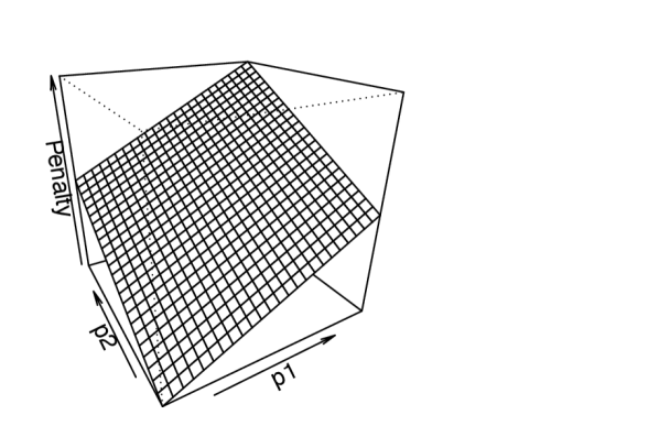
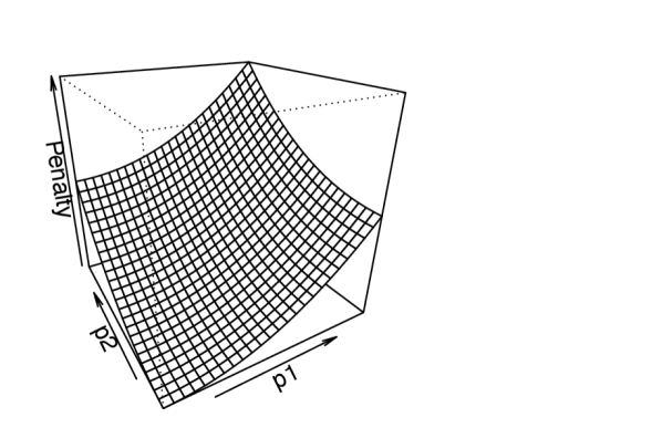
Figure 1: $L_{1}$ norm (left) and $L_{2}$ norm (right) penalty functions for $J=2$ binomial success probabilities.

Note that as $\mathrm{Pen}_{2}(\bm{p})\leq\mathrm{Pen}_{1}(\bm{p})$ for all $\bm{p}\in[0,1]^{I}$, the $L_{1}$ norm will more aggressively shrink success probabilities to $0$ than the $L_{2}$ norm. Due to the resemblance of the $L_{1}$ norm to the commonly-used lasso penalty in regression, it should be pointed out that its application here will not result in shrinkage estimators exactly equal to $0$. In fact, the penalized negative log-likelihood function $D_{1}(\bm{p})=-\ell(\bm{p}|\bm{x})+\lambda\mathrm{Pen}_{1}(\bm{p})$ has unique solution

$$\tilde{p}_{i}=\frac{1}{2}\left(\frac{\lambda_{i}+1}{\lambda_{i}}\right)\left[1-\left(1-\frac{4\lambda_{i}\hat{p}_{i}}{(\lambda_{i}+1)^{2}}\right)^{1/2}\right],\ i=1,\ldots,I$$

where $\lambda_{i}=\lambda/N_{i}$ and $\hat{p}_{i}=x_{i}/N_{i}$ is the unpenalized MLE. While it is not necessarily intuitive from the form of the penalized estimator, it can easily be verified that $0<\tilde{p}_{i}<\hat{p}_{i}$ for all $\lambda>0$. The solution to the $L_{2}$ penalty function is also easy to compute, but no general closed-form expression is possible as it requires solving a cubic polynomial.

The bounded nature of $\mathrm{Pen}_{1}$ and $\mathrm{Pen}_{2}$ in (2) may not appeal to some. One choice of an unbounded penalty is

$$\mathrm{Pen}_{3}(\bm{p})=-\sum_{i}\log(1-p_{i}).$$

This penalty has a lower bound of $0$, but has no upper bound. For an illustration when $I=2$, see Figure 2. The solution to the corresponding penalized likelihood problem is

$$\tilde{p}_{i}=\frac{N_{i}}{N_{i}+\lambda}\hat{p}_{i},\ i=1,\ldots,I.$$

None of the penalties considered so far have the lasso-like property of shrinking parameters to $0$ for a finite value of $\lambda$. However, it is possible to find a penalty that achieves this. Consider

$$\mathrm{Pen}_{4}(\bm{p})=\sum_{i}\log p_{i}$$

also illustrated in Figure 2 for $I=2$. This penalty function is bounded above, but has no lower bound as the individual $p_{i}$’s approach $0$. In fact, this penalty function is not associated with a norm as defined in Section 2.1, putting it somewhat outside the framework in which our estimation problem has been formulated. The latter point notwithstanding, the corresponding penalized likelihood estimator is

$$\tilde{p}_{i}=\left\{\begin{array}[]{ll}\dfrac{N_{i}}{N_{i}-\lambda}\hat{p}_{i}-\dfrac{\lambda}{N_{i}-\lambda}&\lambda\leq x_{i}\\ 0&\lambda>x_{i}\end{array}\right.$$

for $i=1,\ldots,I$. Perhaps this penalty can appropriately be described as “greedy” in the sense that it has the potential to dominate the data and result in a shrinkage estimator equal to $0$ even when there are observed successes suggesting otherwise.

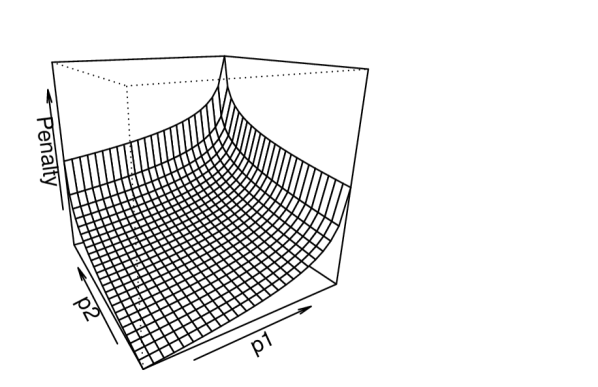
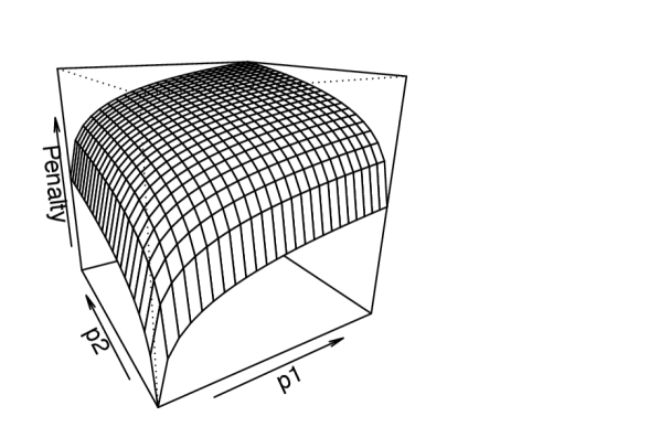
Figure 2: Penalties $\mathrm{Pen}_{3}$ (left) and $\mathrm{Pen}_{4}$ (right) penalty functions, respectively unbounded from above and below, for $I=2$ binomial success probabilities.

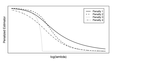
Figure 3: Schematic representation of four different penalized estimators shrinking $\tilde{p}$ closer to $0$.

All four of the penalized solutions above corresponding to some notion of success probabilities being “close to $0$” or “not too large.” Figure 3 shows a schematic representation of the behavior of these estimators as a function of $\log(\lambda)$.

2.3 Other Shrinkage Configurations

The penalized estimators of Section 2.2 all revolve around the goal of ensuring that the estimates $\tilde{p}_{i}$ are close to $0$. If, on the other hand, it was desired to have estimates $\tilde{p}_{i}$ close to $1$, then by symmetry all of the examples considered could replace the $p_{i}$ in each of the penalty functions by $1-p_{i}$. Of course, many other types of penalties could also be of interest. For instance, consider the hypothetical example where a subject-matter expert expresses confidence that all of the $p_{i}$ should be close to some specified value $\kappa\in(0,1)$. For this specified $\kappa$, define

$$\mathrm{Pen}_{5}(\bm{p}|\kappa)=-\sum_{i=1}^{I}\left[\kappa\log(p_{i})+(1-\kappa)\log(1-p_{i})\right].$$

This penalty function has a minimum when all the $p_{i}$ are equal to $\kappa$, and is unbounded above whenever one of the $p_{i}$ approach either $0$ or $1$. This penalty therefore shrinks the $p_{i}$ towards the specified $\kappa$ value. The penalized estimators are

$$\tilde{p}_{i}=\frac{N_{i}}{N_{i}+\lambda}\ \hat{p}_{i}+\frac{\lambda}{N_{i}+\lambda}\ \kappa,\ i=1,\ldots,I.$$

For the $i^{th}$ variable, this estimator is a linear combination of the MLE and $\kappa$. The careful reader may also notice that this estimator has much in common with the Bayesian estimator of a binomial success probability with a beta prior. This example makes clear how the value of $\lambda$ controls whether the strength of evidence lies with the empirical estimator $\hat{p}_{i}$ or with the pre-specified reference $\kappa$. Similarly, say a subject-matter expert states that the success probabilities should all be “close” to one another, but without specifying a $\kappa$ value. For the WRI data, this is equivalent to requiring the $p_{i}$ to be near one another using some appropriate distance metric. For this, define the bounded penalty function

$$\mathrm{Pen}_{L_{2}}(\bm{p})=\sum_{i=1}^{I}\sum_{j=1}^{I}\left(p_{i}-p_{j}\right)^{2}.$$

Alternatively, if an unbounded penalty function is preferred, one could use

$$\mathrm{Pen}_{Q_{2}}(\bm{p})=\sum_{i=1}^{I}\sum_{j=1}^{I}\left[\Phi^{-1}(p_{i})-\Phi^{-1}(p_{j})\right]^{2}$$

where $\Phi^{-1}$ is the standard normal quantile function. Neither of these penalties result in closed-form solutions for the shrinkage estimators $\tilde{p}_{i}$, $i=1,\ldots,I$.

3 Data-Driven Shrinkage

In Section 2, different penalty functions were considered for estimating $I$ independent binomial success probabilities assuming a known value of the shrinkage parameter $\lambda$. As $\lambda$ controls the relative importance of the penalty function, it is important to choose a value resulting in parameter estimates with small MSE. We present here how V-fold cross-validation (VFCV) can be used for selecting an optimal shrinkage parameter. While the VFCV approach is fully defined in this section, the interested reader can consult Arlot and Celisse, (2010) for a more in-depth discussion of this method as well as other cross-validation approaches.

Consider a dataset consisting of $I$ independently sampled variables, with the $i$th variable consisting of $n_{i}$ independent observations. Let $\bm{x}_{i}=(x_{i1},x_{i2},\ldots,x_{in_{i}})$ denote the observations corresponding to the $i$th variable. VFCV partitions the data into $V$ subsets of roughly equal size. For the $i$th variable, let $\mathcal{I}_{i,v}$, $v=1,\ldots,V$ denote a partition of the indices, such that $\bigcup_{v}\ \mathcal{I}_{i,v}=\{1,\ldots,n_{i}\}$ and $\mathcal{I}_{i,v_{1}}\bigcap\mathcal{I}_{i,v_{2}}=\varnothing$ for all $v_{1}\neq v_{2}$ with $v_{1},v_{2}\in\{1,\ldots,V\}$.

VFCV repeatedly creates subsets of the data for model training, in each instance leaving out one of the $V$ subsets per variable. The subsets left out in each iteration are then used for model validation. More specifically, the model building data subsets are used to estimate penalized parameter estimates for various degrees of penalty enforcement, say $M$ possible values of $\lambda$ satisfying $0=\lambda_{1}<\lambda_{2}<\cdots<\lambda_{M}$. The negative log-likelihood function for the validation data is then evaluated using penalized estimators corresponding to each possible value of $\lambda$. The optimal value $\lambda_{opt}$ is chosen to be the minimizer of the negative log-likelihood function averaged over the validation subsets.

Algorithmically, implementation of VFCV proceeds as follows:

• For the $i^{th}$ variable, form a training dataset by excluding the $v$th fold, $\bm{x}_{train,i}^{(v)}=\{x_{ij}:\ j\not\in\mathcal{I}_{i,v}\}$, and let the $v$th fold equal to the validation set, $\bm{x}_{valid,i}^{(v)}=\{x_{ij}:\ j\in\mathcal{I}_{i,v}\}$. Let $n_{i}^{(v)}$ denote the number of observations in $\bm{x}_{train,i}^{(v)}$. Also let $\bm{x}_{train}^{(v)}$ and $\bm{x}_{valid}^{(v)}$ denote the collection of the training and validation sets for all $I$ variables.

• For each value $0=\lambda_{0}<\lambda_{1}<\ldots<\lambda_{M}$, find the estimators $\tilde{\bm{\theta}}_{train}^{(v)}(\lambda_{m})$ that minimize the penalized negative log-likelihood function

  $$D_{k}(\bm{\theta})=-l\left(\bm{\theta}\left|\bm{x}_{train}^{(v)}\right.\right)+\lambda_{m}\bar{n}^{(v)}\mathrm{Pen}(\bm{\theta})$$

  where $\bar{n}^{(v)}=(1/I)\sum_{i}n_{i}^{(v)}$.

• Calculate the validation function by evaluate the negative log-likelihood at this estimator,

  $$\tilde{D}^{(v)}(\lambda_{m})=-\ell\left(\left.\tilde{\bm{\theta}}_{train}^{(v)}(\lambda_{m})\right|\bm{x}_{valid}^{(v)}\right).$$

The above bullets are repeated for $v=1,\ldots,V$ and the VFCV score is defined as

$$\mathrm{CV}_{m}=\mathrm{CV}(\lambda_{m})=\sum_{v=1}^{V}\tilde{D}^{(v)}(\lambda_{m}).$$ (3)

The optimal shrinkage level is taken to be the minimizer of $\mathrm{CV}_{m}$, i.e. $\lambda_{opt}=\lambda_{m^{\ast}}$ with $m^{\ast}=\mathrm{argmin}_{m}\mathrm{CV}_{m}$. Note that after the optimal penalty level has been chosen using VFCV, penalized estimators are calculated one more time using the full dataset. The penalized likelihood estimator with data-driven shrinkage, denoted $\bm{\tilde{\theta}}_{pen}$, is the minimizer of

$$D_{opt}(\bm{\theta})=-\ell(\bm{\theta}|\bm{x})+\lambda_{opt}\,\bar{n}\,\mathrm{Pen}(\bm{\theta})$$

where $\bar{n}=(1/I)\sum_{i}n_{i}$. The literature on cross-validation recommends various choices for $V$, with common values ranging from $V=2$ to $V=10$. The choice $V=n$ is equivalent to leave-one-out cross-validation and can become computationally expensive. As discussed in Arlot and Celisse, (2010), the size of the validation set has an effect on the bias of the penalized estimator, while the number of folds $V$ controls for the variance of the estimated penalization parameter. These authors also discuss some asymptotic considerations of cross-validation. If $n_{train}$ denotes the size of the training set, then for $n_{train}/n\rightarrow 1$, cross-validation is asymptotically equivalent to Mallows’ $C_{p}$ and therefore asymptotically optimal. Furthermore, if $n_{train}/n\rightarrow\gamma\in(0,1)$, then asymptotically the model is equivalent to Mallows’ $C_{p}$ multiplied by (or over-penalized by) a factor $(1+\gamma)/(2\gamma)$. Asymptotics notwithstanding, throughout the remainder of this paper, an approach of $V=10$ is used. This strikes a balance between having larger training sets and reasonable computational costs.

4 Simulation Studies

In Section 2, various shrinkage estimators for the binomial distribution were considered. Of course, the binomial model is not the only count model of interest. In this section, shrinkage estimation is considered for the binomial model as well as two related models, the zero-inflated binomial and the beta-binomial. In most scenarios investigated here, no closed-form solutions for the penalized estimators are available. Even so, these simulation studies are very useful for investigating the properties of different penalty functions and how they impact parameter estimation for the three models. Simulations are restricted to $I=10$ independent variables (passages), consisting of $N_{i}=N=40$ trials (passage length) and having $n_{i}=n=50$ independent observations (students) for $i=1,\ldots,I$. This choice was motivated in large part by the structure of the real data considered in this paper.

4.1 The Binomial Model

In the simulation, samples $\mathcal{X}=\{X_{ij},i=1,\ldots,I,\ j=1,\ldots,n\}$ were generated with independent observations $X_{ij}\sim\mathrm{Bin}(N,p_{i})$ and $(I,N,n)=(10,40,50)$. The binomial success probabilities $p_{i}$ were sampled from a scaled beta distribution. Three shapes of the success probability distribution were considered, namely a skewed distribution $(p_{i}-a)/(b-a)\sim\mathrm{Beta}(2,5)$, a very flat distribution $(p_{i}-a)/(b-a)\sim\mathrm{Beta}(5/4,5/4)$, and a bell-shaped distribution $(p_{i}-a)/(b-a)\sim\mathrm{Beta}(10,10)$. The three success probability distributions are illustrated in Figure 4. When considering shrinkage to $0$, we chose scaling parameters $(a,b)\in\{(0.01,0.05),(0.01,0.10),(0.30,0.50)\}$ and when considering shrinkage closer to one another, we chose $(a,b)\in\{(0.01,0.05),(0.08,0.20),(0.31,0.35)\}$. In total, this makes for $18$ simulation configurations: $3$ distributions for the $p_{i}$ $\times$ $2$ types of shrinkage $\times$ $3$ choices of $(a,b)$ for each shrinkage type. The $\lambda$ term controlling how aggressively the penalty gets enforced was chosen using cross-validation using $63$ possible values ranging from $0$ to $10,000$ spaced approximately equidistant on a logarithmic scale. These $\lambda$ values were selected (after some trial-and-error) to ensure they cover the spectrum of negligible penalization ($\lambda=0$) through the penalty dominating ($\lambda=10,000$). VFCV was used to choose the optimal $\lambda$ for each simulated dataset. In addition to the penalized estimators, maximum likelihood estimators were also calculated. In total, $K=500$ samples were generated for each of the $18$ simulation configurations.

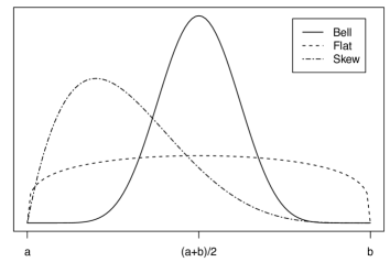
Figure 4: Success probability distributions considered in the simulation study.

Summarized in the tables below are the Monte Carlo estimates of the MSE ratios. For the $k$th sample $\mathcal{X}_{k}$, let $\bm{p}_{k}=\left(p_{k,1},\ldots,p_{k,10}\right)$ denote the true success probabilities simulated from a specified scaled Beta distribution. Let $\hat{\bm{p}}_{k}$ denote the MLE and let $\tilde{\bm{p}}_{k}$ denote a penalized estimator found using VFCV. Define Sum of Squared Deviations $\mathrm{SSD}(\bm{p}_{1},\bm{p}_{2})=\sum_{i=1}^{I}(p_{1i}-p_{2i})^{2}$. The Monte Carlo MSE ratios are subsequently defined as

$$\mathrm{MSE}_{\mathrm{Pen}}=\frac{(1/K)\sum_{k=1}^{K}\mathrm{MSD}(\tilde{\bm{p}}_{k},\bm{p}_{k})}{(1/K)\sum_{k=1}^{K}\mathrm{MSD}(\hat{\bm{p}}_{k},\bm{p}_{k})}$$

where the subscript “$\mathrm{Pen}$” emphasizes the specific penalty function used to obtain the estimators. Maximum likelihood is often considered a “gold standard” estimation method. Therefore, we do not report the estimated MSE values themselves, but rather emphasize the MSE ratios comparing the penalized estimators to maximum likelihood. An MSE ratio less than $1$ indicates superior performance of the penalized estimator, while an MSE ratio exceeding $1$ indicates that the unpenalized estimator is preferred.

In Table 4.1, the results of shrinking success probabilities to zero are presented using the penalties $\mathrm{Pen}_{j}(\bm{p})$, $j=1,\ldots,4$. In Table 4.1, the results of shrinking success probabilities closer to one another using penalties $\mathrm{Pen}_{L_{2}}$ and $\mathrm{Pen}_{Q_{2}}$ are presented. To recall these penalties, consult Section 2.2 of this paper. The tables also report summary measures for the count variables simulated under the different configurations, taking $\bar{\mathrm{E}}(X)=(1/I)\sum_{i=1}^{I}\mathrm{E}(X_{i})$ and $\bar{\mathrm{S}}(X)=\left[(1/I)\sum_{i=1}^{I}\mathrm{Var}(X_{i})\right]^{1/2}$ as summary measures of location and spread.

MSE ratios comparing penalized parameter estimates to maximum likelihood when shrinking estimators to 0. Penalty $p_{i}\in(a,b)$ Shape $\bar{\mathrm{E}}(X)$ $\bar{\mathrm{S}}(X)$ Pen₁ Pen₂ Pen₃ Pen₄ $(0.01,0.05)$ Skew 0.857 0.950 0.999 0.956 0.988 1.382 Flat 1.200 1.158 0.999 0.968 0.995 1.012 Bell 1.200 1.093 0.999 0.961 0.997 1.011 $(0.01,0.10)$ Skew 1.429 1.303 0.999 0.977 0.995 1.013 Flat 2.200 1.726 1.000 0.982 0.994 1.004 Bell 2.200 1.493 1.000 0.978 0.996 1.002 $(0.30,0.50)$ Skew 14.286 3.283 0.998 0.998 1.015 0.999 Flat 16.000 3.749 0.999 0.998 1.037 1.000 Bell 16.000 3.216 1.000 0.999 1.027 1.003

MSE ratios comparing penalized parameter estimates to maximum likelihood when shrinking estimators closer to one another. Penalty $p_{i}\in(a,b)$ Shape $\bar{\mathrm{E}}(X)$ $\bar{\mathrm{S}}(X)$ L₂ Q₂ $(0.01,0.05)$ Skew 0.857 0.950 0.928 0.906 Flat 1.200 1.159 0.935 0.942 Bell 1.200 1.093 0.705 0.704 $(0.08,0.20)$ Skew 4.571 2.149 0.960 0.952 Flat 5.600 2.533 0.969 0.973 Bell 5.600 2.255 0.854 0.856 $(0.31,0.35)$ Skew 12.857 2.965 0.411 0.411 Flat 13.200 3.003 0.652 0.652 Bell 13.200 2.979 0.292 0.293

In Table 4.1, the best-performing penalty function when shrinking to $0$ is $\mathrm{Pen}_{2}(\bm{p})=\sum_{i}p_{i}^{2}$. Even so, the relative improvement in efficiency is small throughout. The only penalty that consistently leads to worse performance than maximum likelihood is $\mathrm{Pen}_{4}(\bm{p})$. Recall that this penalty function is not associated with a norm and is able to very aggressively shrink success probabilities to $0$. This simulation suggests that, at least in the scenarios considered, this penalty shrinks too aggressively. For the other three estimators, VFCV results in penalized estimators with slightly better performance than MLE.

In Table 4.1, the performance of the $L_{2}$ and $Q_{2}$ penalties is nearly indistinguishable. When shrinking parameters closer to one another, large gains in efficiency are sometimes realized. This is especially notable when the Beta shape from which the success probabilities are generated is bell-shaped, i.e. the $p_{i}$ are close to one another. In all instances, VFCV results in penalized estimators with performance superior to maximum likelihood. Altogether, these simulations illustrate that both the average success probability and the spacing of the $p_{i}$ relative to that average are important in determining the reduction in MSE. In Table 2, we also note that the MSE ratio tends to decrease, indicating better efficiency, when $\bar{\mathrm{E}}(X)$ is further from $0$. For penalties shrinking the $p_{i}$ closer to one another, an MSE ratio below $0.3$ was realized, showing dramatic improvement due to shrinkage.

4.2 The Zero-inflated Binomial Distribution

The probability mass function of the zero-inflated binomial (ZIB) distribution is

$$f(x|N,\pi,\gamma)=\left\{\begin{array}[]{ll}\gamma+(1-\gamma)(1-\pi)^{N}&\text{for $x=0$}\\ (1-\gamma)\dbinom{N}{x}\pi^{x}(1-\pi)^{N-x}&\text{for $x=1,\ldots,N$}\end{array}\right.$$

where $\gamma$ represents the excess zero probability, and $\pi$ and $N$ are the binomial success probability and number of trials. For $X\sim\mathrm{ZIB}(N,\pi,\gamma)$, it follows that $E[X]=N\pi(1-\gamma)$. Consequently, we note the overall expected success proportion in a ZIB is $p=E[X]/N=\pi(1-\gamma)$. The parameter $p$ is of primary interest when considering possible penalty functions, especially under the assumption that the different ZIB distributions are “similar” to one another.

In the simulation study, samples $\mathcal{X}=\{X_{ij},i=1,\ldots,I,\ j=1,\ldots,n\}$ were generated with independent ZIB variables, $X_{ij}\sim\mathrm{ZIB}(N,\pi_{i},\gamma_{i})$ and $(I,N,n)=(10,40,50)$. The overall success proportions $p_{i}$ and the excess zero probabilities $\gamma_{i}$ were sampled from the scaled beta distributions as per Figure 4 with the specific bounds $(a_{1},b_{1})$ for the $p_{i}$ and $(a_{2},b_{2})$ for the $\gamma_{i}$ listed in the table below. In total, $12$ simulation configurations were considered: $3$ distributional shapes $\times$ $4$ choices for $(a_{1},b_{1},a_{2},b_{2})$. In the simulations, the binomial success probabilities $\pi_{i}$ were recovered from the $p_{i}$ and $\gamma_{i}$ through $\pi_{i}=p_{i}/(1-\gamma_{i})$, $i=1,\ldots,I$. A total of $k=500$ samples were simulated under each configuration.

The ZIB simulation considered three penalty functions, $\mathrm{Pen}_{2}(\bm{p})=\sum_{i}p_{i}^{2}$, $\mathrm{Pen}_{L_{2}}(\bm{p})=\sum_{i}\sum_{j}(p_{i}-p_{j})^{2}$, and $\mathrm{Pen}_{full}(\bm{\gamma},\bm{\pi})=\sum_{i}\sum_{j}(\gamma_{i}-\gamma_{j})^{2}+\sum_{i}\sum_{j}(\pi_{i}-\pi_{j})^{2}$. The first of these, termed zero shrinkage, results in estimated $p_{i}$ closer to $0$. The second, termed mean shrinkage, results in $p_{i}$ closer to one another. The third, termed full shrinkage, shrinks all $\gamma_{i}$ closer to one another and all $\pi_{i}$ closer to one another. While both the penalties $\mathrm{Pen}_{L_{2}}$ and $\mathrm{Pen}_{full}$ have the goal of estimating models that are “similar” to one another, the second penalty is much more strict. To see this, consider two passages with equal average difficulty $p_{i}=p_{j}$. Under the first penalty, the contribution of their squared difference is $0$. However, it is possible to have $(\gamma_{i},\pi_{i})\neq(\gamma_{j},\pi_{j})$ even when $p_{i}=p_{j}$, meaning there could conceivably be a non-zero contribution to the full shrinkage penalty function.

In addition to using VFCV to select the level of shrinkage for the above three penalities, a combined estimator, termed minCV, was calculated by selecting among the three penalized estimators the one with the smallest VFCV score. The same set of $63$ $\lambda$ values ranging from $0$ to $10,000$ were used. The Monte Carlo MSE ratios for the success proportions $\bm{p}$ are in Table 4.2. The MSE ratios for $\bm{\gamma}$ and $\bm{\pi}$ were also calculated, and these can be found in Table 8 of the Supplemental Material.

MSE ratios for ZIB success proportions $\bm{p}=(p_{1},\ldots,p_{10})$ comparing penalized parameter estimates to maximum likelihood for different penalization approaches. Penalty $\pi_{i}\in(a_{1},b_{1})$ $\gamma_{i}\in(a_{2},b_{2})$ Shape $\bar{\mathrm{E}}(X)$ $\bar{\mathrm{S}}(X)$ Zero Mean Full minCV $(0.01,0.05)$ $(0.10,0.14)$ Skew 0.761 0.935 0.957 0.888 0.981 0.958 Flat 1.055 1.153 0.977 0.942 0.979 0.983 Bell 1.056 1.097 0.964 0.668 0.836 0.755 $(0.04,0.06)$ $(0.20,0.30)$ Skew 1.410 1.395 0.968 0.364 0.368 0.356 Flat 1.502 1.485 0.971 0.562 0.526 0.523 Bell 1.496 1.477 0.968 0.258 0.246 0.239 $(0.15,0.30)$ $(0.04,0.06)$ Skew 7.364 3.064 1.006 0.969 0.860 0.885 Flat 8.551 3.586 1.010 1.005 0.808 0.819 Bell 8.552 3.296 1.009 0.821 0.873 0.899 $(0.05,0.06)$ $(0.20,0.70)$ Skew 1.389 1.526 0.963 0.203 0.635 0.273 Flat 1.209 1.531 0.955 0.223 0.934 0.259 Bell 1.210 1.529 0.951 0.183 0.372 0.245

Consider now Table 4.2. While zero shrinkage does result in some efficiency gains in most scenarios, overall MSE ratios close to $1$ suggest little improvement from using this penalty. On the other hand, both mean and full shrinkage result in large decreases in the MSE ratios. Overall, it cannot be said that either mean and full shrinkage performs best. This makes sense, as it depends on the configuration of all parameters and not just the mean parameters. Finally, while minCV does not always have the smallest MSE ratio, it is generally close to the minimum. This suggests that data-driven selection of the level of shrinkage as well as the penalty function leads to good performance for the model.

4.3 The Beta-Binomial Model

The probability mass function of the beta-binomial distribution is given by

$$f(x|N,\alpha,\beta)=\binom{N}{x}\frac{B(x+\alpha,N-x+\beta)}{B(\alpha,\beta)},\ x=0,1,...,N$$

where $B(x,y)=\int_{0}^{1}t^{x-1}(1-t)^{y-1}dt$ is the so-called Beta function, $N$ is the number of trials, and $\alpha>0$ and $\beta>0$ control the mean and variance of the distribution. Defining $p=\alpha/(\alpha+\beta)\in(0,1)$ and $\nu=(\alpha+\beta+N)/(\alpha+\beta+1)\in(1,N)$, the mean and variance of the distribution can be written as $E[X]=Np$ and $Var[X]=Np(1-p)\nu$. In this parameterization, $p$ and $\nu$ denote, respectively, the expected success proportion successes and the the over-dispersion relative to a binomial distribution with the same mean value.

Samples $\mathcal{X}=\{X_{ij},i=1,\ldots,I,\ j=1,\ldots,n\}$ were generated with independent Beta-Binomial variables, $X_{ij}\sim\mathrm{BetaBin}(N,\alpha_{i},\beta_{i})$, with $(I,N,n)=(10,40,50)$. The overall success proportions $p_{i}$ and the overdispersion measures $\nu_{i}$ were sampled from the scaled beta distributions as per Figure 4 with the specific bounds $(a_{1},b_{1})$ for the $p_{i}$ and $(a_{2},b_{2})$ for the $\nu_{i}$ listed in Table 4.3. Again, $12$ simulation configurations were considered. In the simulation, parameters $\alpha_{i}$ and $\beta_{i}$ for the beta-binomial distribution were recovered from the simulated $p_{i}$ and $\nu_{i}$ through the relationships in the preceding paragraph. A total of $K=500$ samples were simulated under each configuration.

As in Section 4.2, three penalty functions. Letting $p_{i}=\alpha_{i}/(\alpha_{i}+\beta_{i})$, $i=1,\ldots,I$, these were $\mathrm{Pen}_{2}(\bm{p})=\sum_{i}p_{i}^{2}$, $\mathrm{Pen}_{L_{2}}(\bm{p})=\sum_{i}\sum_{j}(p_{i}-p_{j})^{2}$, and $\mathrm{Pen}_{full}(\bm{\alpha},\bm{\beta})=\sum_{i}\sum_{j}(\alpha_{i}-\alpha_{j})^{2}+\sum_{i}\sum_{j}(\beta_{i}-\beta_{j})^{2}$. These are again termed, respectively, zero shrinkage, mean shrinkage, and full shrinkage. In addition to the three penalized estimators, an estimator termed minCV was calculated by selecting among the three penalized estimators the one with the smallest CV score. The MSE ratios for all estimators are reported in Table 4.3. The table shows the results for the success proportions $\bm{p}$, and the equivalent results for $\bm{\alpha}$ and $\bm{\beta}$ can be found in Table 9 of the Supplemental Material.

MSE ratios for Beta-Binomial success proportions $\bm{p}=(p_{1},\ldots,p_{10})$ comparing penalized parameter estimates to maximum likelihood for different penalization approaches. Penalty $p_{i}\in(a_{1},b_{1})$ $\nu_{i}\in(a_{2},b_{2})$ Shape $\bar{\mathrm{E}}(X)$ $\bar{\mathrm{S}}(X)$ Zero Mean Full minCV $(0.05,0.10)$ $(4,6)$ Skew 2.361 3.102 0.917 0.474 0.428 0.429 Flat 2.733 3.480 0.928 0.702 0.591 0.604 Bell 2.730 3.455 0.921 0.290 0.270 0.271 $(0.12,0.22)$ $(2,5)$ Skew 5.742 3.755 0.974 0.722 0.726 0.708 Flat 6.513 4.419 0.977 0.903 0.948 0.889 Bell 6.515 4.327 0.973 0.476 0.466 0.463 $(0.17,0.22)$ $(3,8)$ Skew 6.947 4.929 0.971 0.301 0.400 0.331 Flat 7.230 5.557 0.971 0.445 0.762 0.481 Bell 7.221 5.555 0.968 0.217 0.242 0.227 $(0.05,0.06)$ $(2,10)$ Skew 1.952 2.723 0.905 0.170 0.469 0.211 Flat 1.943 3.139 0.891 0.188 0.733 0.213 Bell 1.949 3.183 0.893 0.155 0.187 0.175

Inspecting Table 4.3, zero shrinkage is noted to be the least effective approach here, even while still being more effective than maximum likelihood. For most of the simulation configurations, MSE ratios under mean and full shrinkage are comparable. Here, the minCV approach is also very impressive, in most instances nearly matching the best-performing method. This reaffirms that VFCV can be effectively used to choose both the level of shrinkage for a specific penalty function, but then also choose from among competing penalty functions.

5 Data Analysis

The methodology developed in this paper was motivated by the oral reading fluency data collected from a sample of $508$ elementary-school aged children. Each child was randomly assigned one of ten available passages to read. This resulted in around 50 Words Read Incorrectly (WRI) scores per passage. Table 5 reports specific details for passage length, sample size per passage, as well as the minimum, median, and maximum WRI scores. Of interest is to accurately and efficiently estimate passage difficulty as measured by the average proportion of words read incorrectly. Note that higher WRI proportions (i.e. WRI counts divided by passage length) indicate that a passage is more difficult. Figure 5 provides information about the passage-specific WRI proportions. The solid dot in each violin plot represents the mean WRI proportion. The means correspond to the unpenalized maximum likelihood estimates of passage difficulty.

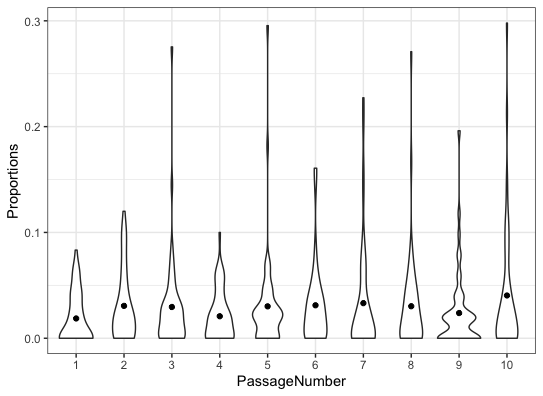
Figure 5: WRI proportions for the ten passages

Passage-level summary statistics Passage Number 1 2 3 4 5 6 7 8 9 10 Sample Size 49 51 51 50 52 51 50 53 51 50 Passage Length 48 50 69 50 44 56 44 48 51 47 Minimum WRI 0 0 0 0 0 0 0 0 0 0 Median WRI 0 1 1 1 1 1 1 1 1 1 Maximum WRI 4 6 19 5 13 9 10 13 10 14

The mean WRI proportions in Figure 5 appear fairly close to one another, supporting the assumption that the passages fall within a narrow range of difficulty. Thus, it is plausible that appropriate shrinkage will result in improved estimates of difficulty.

Three models and three types of shrinkage were considered for the data at hand. We remind the reader that classic selection criteria such as AIC and BIC cannot easily be applied in parameter shrinkage settings unless one is able to calculate the effective number of parameters. In a penalized model with $K$ specified parameters, the effective number of parameters $\tilde{K}$ can be dramatically smaller than $K$. Generally, there is no easy way to calculate $\tilde{K}$ in penalized models. We therefore used cross-validation (CV) to select the best model, noting that such CV scores as per Geisser, (1975) represent a discrepancy measure for each model. The lowest CV score corresponds to the smallest empirical discrepancy between observed data and estimated model. Therefore, the smallest CV score corresponds to the optimal model choice. In each model under consideration, the same set of data partitions was used to select a smoothing parameter with VFCV with $V=10$ fold. Table 5 reports the VFCV scores as defined in (3). When the penalty in the table is specified as “None”, the VFCV score corresponds to the unpenalized maximum likelihood estimators.

10-fold CV scores and optimal $\lambda$ values for the three distributions considered. Distribution Penalty VFCV $\log(\lambda_{opt}+1)$ Binomial None $1025.5$ – Zero $1024.9$ $3.56$ Mean $1017.1$ $4.36$ ZIB None $964.7$ – Zero $964.3$ $2.78$ Mean $959.6$ $3.96$ Full $950.4$ $3.56$ BetaBin None $869.7$ – Zero $869.5$ $2.41$ Mean $866.3$ $3.56$ Full $851.9$ $0.04$

Beta-binomial parameter estimates for the WRI data. Maximum Likelihood Mean Shrinkage Full Shrinkage Passage $\hat{\alpha}$ $\hat{\beta}$ $\hat{p}$ $\tilde{\alpha}$ $\tilde{\beta}$ $\tilde{p}$ $\tilde{\alpha}$ $\tilde{\beta}$ $\tilde{p}$ P1 1.28 66.34 0.019 1.20 52.67 0.022 0.70 27.45 0.025 P2 1.51 45.15 0.032 1.50 47.47 0.031 0.91 27.44 0.032 P3 0.84 19.85 0.040 0.80 22.81 0.034 0.96 27.44 0.034 P4 2.47 160.0 0.015 2.25 123.5 0.018 0.67 27.45 0.024 P5 1.17 42.54 0.027 1.17 41.65 0.027 0.83 27.45 0.030 P6 1.18 29.10 0.039 1.13 32.52 0.034 0.97 27.44 0.034 P7 0.53 19.48 0.026 0.53 18.75 0.027 0.74 27.44 0.026 P8 0.87 25.37 0.033 0.86 27.20 0.031 0.88 27.44 0.031 P9 0.85 32.25 0.026 0.84 30.74 0.027 0.79 27.45 0.028 P10 0.65 17.03 0.037 0.63 19.14 0.032 0.89 27.44 0.031

It is evident from Table 5 that all variations of the beta-binomial model have much lower cross-validation scores than either the binomial or zero-inflated binomial models. Furthermore, VFCV never selects unpenalized maximum likelihood model for any of the distributions considered. With regards to penalty type, full shrinkage works best for this model with mean shrinkage being a distant second choice. Table 5 shows the beta-binomial parameter estimates obtained using maximum likelihood as well as penalized likelihood with mean shrinkage and full shrinkage. It is interesting to note that in the full shrinkage solution, the $\tilde{\beta}_{i}$ values have all been shrunk to within $0.01$ of a common value, but the $\tilde{\alpha}_{i}$ still exhibit a fair spread of values. For unpenalized maximum likelihood, the estimated success proportions range from $0.019$ to $0.04$, while the full shrinkage values range from $0.024$ to $0.034$. The latter shows much more adherence to the idea that the passages are similar in terms of difficulty.

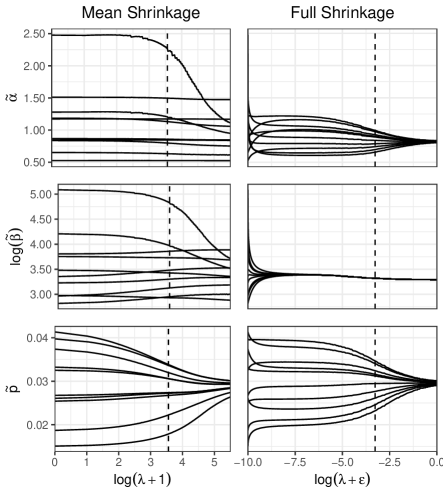
Figure 6: Beta-binomial parameter estimates under mean shrinkage and full shrinkage. Dashed line indicates optimal shrinkage. Scale value to improve full shrinkage plot readability is $\varepsilon=e^{-10}$.

For the interested reader, Figure 6 shows the penalized likelihood estimate trajectories for mean shrinkage and full shrinkage as a function of $\lambda$. The estimates of $\tilde{\beta}$ are presented on a logarithmic scale. For mean shrinkage, the horizontal scale is $\log(\lambda+1)$ and for full shrinkage it is $\log(\lambda+\varepsilon)$ with $\varepsilon=10^{-10}$. These adjustments were all made to improve readability of the plots. Dashed vertical lines indicate the optimal shrinkage solutions as determined by VFCV.

Under mean shrinkage, the passage-specific $\tilde{\alpha}_{i}$ and $\tilde{\beta}_{i}$ still exhibit a large spread even when the success proportions $\tilde{p}_{i}=\tilde{\alpha}_{i}/(\tilde{\alpha}_{i}+\tilde{\beta}_{i})$ are close to one another. Under full shrinkage, the $\tilde{\beta}_{i}$ values are very quickly shrunk to a nearly common value while the $\tilde{\alpha}_{i}$ still exhibit some spread.

One last matter that we will briefly address is that of post-selection model checking. Using VFCV above, the penalized beta-binomial model with full parameter shrinkage has been selected as the best model in a relative sense. If one wishes to evaluate how well the model fits in an absolute sense, one might compare the empirical and penalized model-based pmfs or cdfs. Figure 7 shows both of these comparisons using the Passage 2 data as an example. These figures are presented with a note of caution – the penalized model-based probabilities will almost never be as close to the empirical probabilities as the unpenalized probabilities based on the same parametric model and estimated for that specific passage only i.e. ignoring the data from other passages. As such, rather than a visual inspection, one may wish to use a more formal diagnostic tool. Pearson’s chi-square goodness-of-fit statistic is one possibility worth considering. The use of this statistic is complicated by two matters. Firstly, as per Chernoff and Lehmann, (1954), the Pearson statistic no longer has a limiting $\chi^{2}$ distribution when evaluated using estimated model parameters. Secondly, the effect of parameter penalization and model selection will further impact the distribution of the statistic. Therefore, to find sensible critical values, one would have to rely on a Monte Carlo procedure that incorporates both penalization and selection. This is a computationally burdensome procedure that we do not further consider in the present paper.

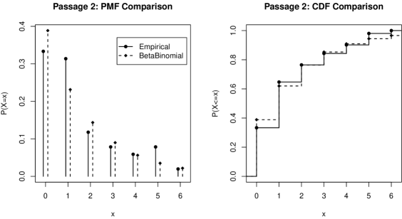
Figure 7: Empirical and penalized model-based pmf and cdf comparisons for the Passage 2 data.

6 Conclusions

The goal of this project was defining and exploring penalized parameter estimators of passage difficulty from independent multivariate count data. WRI scores realized by $508$ students during an ORF assessment motivated the work and these data were analyzed in Section 5. The simulation results presented show that across the different count distributions and simulation configurations considered, large decreases in MSE relative to unpenalized maximum likelihood were often achieved. There is also very little risk in using penalized likelihood, as V-fold cross validation never resulted in a large increase in MSE. In fact, the minCV approach explored in the simulations point the cross-validation being able to choose not just the appropriate level of shrinkage, but also the most appropriate penalty function under consideration. When applying the methodology to the observed WRI data, a penalized beta-binomial model is selected. This choice results in penalized estimators of the passage difficulty with a much tighter spread. This affirms the expectation that the passages are similar in difficulty, with estimated difficulty scores ranging from $2.4\%$ to $3.4\%$. Even so, this does highlight one important avenue for future research. If students are reading different passages to assess ORF, it is desirable to have a method that standardizes WRI scores to be independent of passage difficulty. In practice, students also typically read multiple passages, so exploring methods accounting for correlated WRI scores need to be considered in future.

Supplemental Material

In the main paper, simulation results are only presented for the success proportion estimates $\tilde{p}_{i}$. Of course, it is reasonable to assess the effect of shrinkage on other model parameters as well. The MSE ratios as defined in Section 3 are presented here when estimating the parameters $(\gamma_{i},\pi_{i})$ in the zero-inflated binomial model, see Table 7, and when estimating the parameters $(\alpha_{i},\beta_{i})$ in the beta-binomial model, see Table 8. These results confirm that shrinkage can be very beneficial to the estimation of incidental model parameters as well.

MSE ratios for Zero-Inflated Binomial success proportions $\bm{\gamma}$ and $\bm{\pi}$ comparing penalized parameter estimates to maximum likelihood for different penalization approaches. $\gamma_{i}$ $\pi_{i}$ $p_{i}\in(a_{1},b_{1})$ $\gamma_{i}\in(a_{2},b_{2})$ Shape Zero Mean Full Min CV Zero Mean Full Min CV (0.01,0.05) (0.10,0.14) Skew 1.027 1.000 0.647 0.741 0.947 0.979 0.890 0.928 Flat 1.021 0.992 0.551 0.606 0.973 0.979 0.893 0.921 Bell 1.033 0.998 0.834 0.959 0.964 0.845 0.894 0.889 (0.04,0.06) (0.20,0.30) Skew 1.024 0.855 0.171 0.238 0.979 0.692 0.430 0.446 Flat 1.022 0.868 0.252 0.336 0.981 0.800 0.698 0.701 Bell 1.022 0.770 0.130 0.167 0.980 0.659 0.302 0.318 (0.15,0.30) (0.04,0.06) Skew 1.029 1.059 0.434 0.495 0.998 0.945 1.069 1.071 Flat 1.031 1.047 0.471 0.494 0.997 0.971 1.038 1.039 Bell 1.036 1.009 0.394 0.487 0.998 0.871 1.190 1.204 (0.05,0.06) (0.20,0.70) Skew 1.010 0.610 0.775 0.710 0.983 0.710 0.926 0.779 Flat 0.994 0.517 0.905 0.551 0.991 0.794 0.982 0.805 Bell 0.993 0.478 0.567 0.535 0.985 0.739 0.760 0.746

MSE ratios for Beta-Binomial success proportions $\bm{\alpha}=(\alpha_{1},\ldots,\alpha_{10})$ and $\bm{\beta}=(\beta_{1},\ldots,\beta_{10})$ comparing penalized parameter estimates to maximum likelihood for different penalization approaches. $\alpha_{i}$ $\beta_{i}$ $p_{i}\in(a_{1},b_{1})$ $\nu_{i}\in(a_{2},b_{2})$ Shape Zero Mean Full Min CV Zero Mean Full Min CV (0.05,0.10) (4,6) Skew 0.993 0.922 0.201 0.319 1.037 0.718 0.097 0.192 Flat 0.991 0.932 0.318 0.41 1.037 0.792 0.171 0.254 Bell 0.992 0.922 0.144 0.209 1.039 0.662 0.071 0.119 (0.12,0.22) (2,5) Skew 0.995 0.98 0.69 0.85 1.006 0.954 0.637 0.81 Flat 0.997 1.015 0.999 1.015 1.006 1.01 0.999 1.01 Bell 0.993 0.917 0.186 0.373 1.014 0.845 0.154 0.322 (0.17,0.22) (3,8) Skew 0.992 0.928 0.593 0.746 1.017 0.832 0.544 0.664 Flat 0.994 0.96 1.077 1.019 1.011 0.91 1.058 0.958 Bell 0.991 0.931 0.283 0.401 1.021 0.791 0.241 0.333 (0.05,0.06) (2,10) Skew 0.993 0.988 0.934 0.99 1.017 0.866 0.901 0.866 Flat 0.996 0.958 1.015 0.96 1.007 0.787 1.007 0.788 Bell 0.992 0.91 0.376 0.517 1.046 0.557 0.229 0.306

References

- Agresti and Hitchcock, (2005) Agresti, A. and Hitchcock, D. B. (2005). Bayesian inference for categorical data analysis. Statistical Methods and Applications, 14(3):297–330.
- Allington, (1983) Allington, R. L. (1983). Fluency: The neglected reading goal. The reading teacher, 36(6):556–561.
- Arlot and Celisse, (2010) Arlot, S. and Celisse, A. (2010). A survey of cross-validation procedures for model selection. Statistics surveys, 4:40–79.
- Baklizi and Abu Dayyeh, (2003) Baklizi, A. and Abu Dayyeh, W. (2003). Shrinkage estimation of p (y¡ x) in the exponential case. Communications in Statistics-Simulation and Computation, 32(1):31–42.
- Chernoff and Lehmann, (1954) Chernoff, H. and Lehmann, E. (1954). The use of maximum likelihood estimates in 2 tests for goodness of fit. The Annals of Mathematical Statistics, pages 579–586.
- Datta and Dunson, (2016) Datta, J. and Dunson, D. B. (2016). Bayesian inference on quasi-sparse count data. Biometrika, 103(4):971–983.
- DiSalle and Rasinski, (2017) DiSalle, K. and Rasinski, T. (2017). Impact of short-term intense fluency instruction on students’ reading achievement: A classroom-based, teacher-initiated research study. Journal of Teacher Action Research, 3(2):1–13.
- Efron and Morris, (1973) Efron, B. and Morris, C. (1973). Stein’s estimation rule and its competitors—an empirical bayes approach. Journal of the American Statistical Association, 68(341):117–130.
- Fuchs et al., (2001) Fuchs, L. S., Fuchs, D., Hosp, M. K., and Jenkins, J. R. (2001). Oral reading fluency as an indicator of reading competence: A theoretical, empirical, and historical analysis. Scientific studies of reading, 5(3):239–256.
- Geisser, (1975) Geisser, S. (1975). The predictive sample reuse method with applications. Journal of the American statistical Association, 70(350):320–328.
- Gruber, (2017) Gruber, M. H. (2017). Improving efficiency by shrinkage: the James-Stein and ridge regression estimators. Routledge.
- Hansen, (2016) Hansen, B. E. (2016). Efficient shrinkage in parametric models. Journal of Econometrics, 190(1):115–132.
- Hasbrouck and Tindal, (2006) Hasbrouck, J. and Tindal, G. A. (2006). Oral reading fluency norms: A valuable assessment tool for reading teachers. The reading teacher, 59(7):636–644.
- Hastie et al., (2019) Hastie, T., Tibshirani, R., and Wainwright, M. (2019). Statistical learning with sparsity: the lasso and generalizations. Chapman and Hall/CRC.
- Hoerl and Kennard, (1970) Hoerl, A. E. and Kennard, R. W. (1970). Ridge regression: Biased estimation for nonorthogonal problems. Technometrics, 12(1):55–67.
- Jani, (1991) Jani, P. (1991). A class of shrinkage estimators for the scale parameter of the exponential distribution. IEEE Transactions on Reliability, 40(1):68–70.
- Johns and Lunn, (1983) Johns, J. L. and Lunn, M. K. (1983). The informal reading inventory: 1910–1980. Literacy Research and Instruction, 23(1):8–19.
- (18) Lemmer, H. (1981a). From ordinary to bayesian shrinkage estimators. South African Statistical Journal, 15(1):57–72.
- (19) Lemmer, H. (1981b). Note on shrinkage estimators for the binomial distribution. Communications in statistics-theory and methods, 10(10):1017–1027.
- Månsson, (2013) Månsson, K. (2013). Developing a liu estimator for the negative binomial regression model: method and application. Journal of Statistical Computation and Simulation, 83(9):1773–1780.
- Miura Wayman et al., (2007) Miura Wayman, M., Wallace, T., Wiley, H. I., Tichá, R., and Espin, C. A. (2007). Literature synthesis on curriculum-based measurement in reading. The Journal of Special Education, 41(2):85–120.
- Pandey and Upadhyay, (1985) Pandey, M. and Upadhyay, S. (1985). Bayes shrinkage estimators of weibull parameters. IEEE transactions on reliability, 34(5):491–494.
- Park and Casella, (2008) Park, T. and Casella, G. (2008). The bayesian lasso. Journal of the American Statistical Association, 103(482):681–686.
- Polson and Sokolov, (2019) Polson, N. G. and Sokolov, V. (2019). Bayesian regularization: From tikhonov to horseshoe. Wiley Interdisciplinary Reviews: Computational Statistics, 11(4):e1463.
- Qasim et al., (2020) Qasim, M., Kibria, B., Månsson, K., and Sjölander, P. (2020). A new poisson liu regression estimator: method and application. Journal of Applied Statistics, 47(12):2258–2271.
- Samuels, (1988) Samuels, S. J. (1988). Decoding and automaticity: Helping poor readers become automatic at word recognition. The reading teacher, 41(8):756–760.
- Schreiber, (1991) Schreiber, P. A. (1991). Understanding prosody’s role in reading acquisition. Theory into practice, 30(3):158–164.
- Shinn et al., (1992) Shinn, M. R., Knutson, N., Good III, R. H., Tilly III, W. D., and Collins, V. L. (1992). Curriculum-based measurement of oral reading fluency: A confirmatory analysis of its relation to reading. School Psychology Review, 21(3):459–479.
- Stein et al., (1956) Stein, C. et al. (1956). Inadmissibility of the usual estimator for the mean of a multivariate normal distribution. In Proceedings of the Third Berkeley Symposium on Mathematical Statistics and Probability, Volume 1: Contributions to the Theory of Statistics. The Regents of the University of California.
- Tibshirani, (1996) Tibshirani, R. (1996). Regression shrinkage and selection via the lasso. Journal of the Royal Statistical Society: Series B (Methodological), 58(1):267–288.
- Zandi et al., (2021) Zandi, Z., Bevrani, H., and Arabi Belaghi, R. (2021). Using shrinkage strategies to estimate fixed effects in zero-inflated negative binomial mixed model. Communications in Statistics-Simulation and Computation, pages 1–22.