Efficient experimental characterization of quantum processes via compressed sensing on an NMR quantum processor

Abstract

We employ the compressed sensing (CS) algorithm and a heavily reduced data set to experimentally perform true quantum process tomography (QPT) on an NMR quantum processor. We obtain the estimate of the process matrix $\chi$ corresponding to various two- and three-qubit quantum gates with a high fidelity. The CS algorithm is implemented using two different operator bases, namely, the standard Pauli basis and the Pauli-error basis. We experimentally demonstrate that the performance of the CS algorithm is significantly better in the Pauli-error basis, where the constructed $\chi$ matrix is maximally sparse. We compare the standard least square (LS) optimization QPT method with the CS-QPT method and observe that, provided an appropriate basis is chosen, the CS-QPT method performs significantly better as compared to the LS-QPT method. In all the cases considered, we obtained experimental fidelities greater than 0.9 from a reduced data set, which was approximately five to six times smaller in size than a full data set. We also experimentally characterized the reduced dynamics of a two-qubit subsystem embedded in a three-qubit system, and used the CS-QPT method to characterize processes corresponding to the evolution of two-qubit states under various $J$-coupling interactions.

I Introduction

An essential task in experimental quantum information processing is the characterization of quantum states and their dynamics, which is typically achieved via quantum state tomography (QST) Li et al. (2017) and quantum process tomography (QPT)Chuang and Nielsen (1997). The experimental resources required to implement QST and QPT grow exponentially with the size of system, which makes these methods infeasible beyond a few qubitsMohseni et al. (2008). Hence developing techniques to reduce the experimental resources required for quantum process tomography is of paramount importance in scaling up quantum technologies. Several strategies have been designed to address these issues, such as methods based on the least-square (LS) linear inversion techniqueMiranowicz et al. (2014), linear regression estimationQi et al. (2017), maximum likelihood estimation (MLE)James et al. (2001), self-guided tomographyRambach et al. (2021) and numerical strategiesKaznady and James (2009). Several QST protocols have been extended to perform QPT, which include MLE-based QPTO${}^{{}^{\prime}}$Brien et al. (2004), LS-based QPTSurawy-Stepney et al. (2021), simplified QPTBranderhorst et al. (2009), convex optimization-based QPTHuang et al. (2020), selective and efficient QPT Perito et al. (2018), adaptive QPTPogorelov et al. (2017), and ancilla-assisted QPTAltepeter et al. (2003). These protocols have been successfully demonstrated on various physical systems such as NMR Gaikwad et al. (2018); Xin et al. (2019, 2020); Gaikwad et al. (2021); Zhao et al. (2021), NV-centersZhang et al. (2014), linear opticsSchmiegelow et al. (2010), superconducting qubitsNeeley et al. (2008); Chow et al. (2009); Gaikwad et al. and ion trap-based quantum processorsRiebe et al. (2006).

Methods such as Monte-Carlo process certificationda Silva et al. (2011) and randomized benchmarkingKnill et al. (2008) have been developed to address scalability issues in standard QST and QPT methods. However, they are limited in scope as they do not provide the full process matrix and hence cannot be used to identify gate errors or improve gate fidelity. Other methods such as ancilla-assisted QPT are able to significantly reduce the experimental complexity, however the issues of scalability remain. The CS algorithm borrows ideas from classical signal processing which posits that even heavily undersampled sparse signals can be efficiently reconstructed. The CS algorithm relies on reformulating QST and QPT tasks as a constrained convex optimization problem, and is able to perform complete and true characterization of a given quantum process from a heavily reduced data set without performing actual projective measurements, and does not need any extra resources such as ancilla qubits. CS-QST and CS-QPT have been successfully used to reconstruct unknown quantum states from NMR data Yang et al. (2017), to characterize quantum gates based on superconducting Xmon and phase qubits Rodionov et al. (2014), and to perform efficient estimation of process matrices of photonic two-qubit gates Shabani et al. (2011).

In this work we utilize the CS algorithm to perform QPT of various two- and three-qubit quantum gates on an NMR quantum processor. We also demonstrate the efficacy of the CS-QPT protocol in characterizing two-qubit dynamics in a three-qubit system. We experimentally estimate the full process matrix corresponding to a given quantum process with a high fidelity, from a drastically reduced set of initial states and outcomes. The CS-QPT algorithm is able to efficiently characterize a given quantum process provided the corresponding process matrix is sufficiently sparse (i.e. most of its matrix elements are zero). We use two different operator basis sets to estimate the process matrix using the CS algorithm, namely, the standard Pauli basis and the Pauli-error basis (where the process matrix is maximally sparse Rodionov et al. (2014), i.e. it contains only one non-zero element). We also compare the performance of the CS-QPT and the LS-QPT methods using significantly reduced data sets in both the standard Pauli basis and the Pauli-error basis. We obtained experimental fidelities of greater than 0.9 from a reduced data set of a size approximately 5 to 6 times smaller than the size of a full data set, and our results indicate that the CS-QPT method is significantly more efficient than standard QPT methods.

This paper is organized as follows: In Section II we detail the implementation of the CS algorithm in the context of QPT. The standard QPT protocol is briefly described in Section II.1, while the CS-QPT method is given in Section II.2. Section III describes the experimental implementation of the CS-QPT methods using two and three NMR qubits. In Sections III.1 and III.2, we present the quantum circuit and the corresponding NMR implementation of the CS-QPT method for two- and three-qubit quantum gates, respectively. Section III.3 contains a description of the CS-QPT implementation to capture two-qubit quantum dynamics embedded in a three-qubit system. Section III.4 contains a comparison of the CS-QPT and LS-QPT protocols. Section IV contains a few concluding remarks.

II QPT for a reduced data set

II.1 Standard QPT and $\chi$ matrix representation

In a fixed basis set $\{E_{i}\}$, a quantum map (a completely positive map) $\Lambda$ can be written as Kraus et al. (1983):

$$\Lambda(\rho)=\sum_{m,n}\chi_{mn}E_{m}\rho E_{n}^{\dagger}$$ (1)

where the Kraus operators are expanded as $A_{i}=\sum_{k}a_{ik}E_{k}$ and the quantities $\chi_{mn}=\sum_{i}a_{im}a_{in}^{*}$ are the elements of the process matrix $\chi$ characterizing the quantum map $\Lambda$. In a $d$-dimensional Hilbert space, $\chi$ is a $d^{2}\times d^{2}$ dimensional positive semi-definite matrix and $d^{4}$ real independent parameters are required to uniquely represent it. The number of required parameters reduces from $d^{4}$ to ($d^{4}-d^{2}$) for trace preserving processes O${}^{{}^{\prime}}$Brien et al. (2004).

The standard QPT protocol estimates the complete $\chi$ matrix by preparing the system in different quantum states, letting it evolve under the given quantum process, and then measuring a set of observables Childs et al. (2001). The full data set for QPT can be acquired using tomographically complete sets of input states $\{\rho_{1},\rho_{2},....,\rho_{k}\}$, letting them undergo the desired quantum process $\chi$, and measuring an observable $M$ from the set of measurement operators $\{M_{1},M_{2},...,M_{l}\}$, leading to:

$$B^{i}_{j}=\text{Tr}(M_{j}\Lambda(\rho_{i}))=\sum_{m,n}\chi_{mn}\text{Tr}(M_{j}E_{m}\rho_{i}E_{n}^{\dagger})$$ (2)

For all input states $\{\rho_{i}\}$ and measurement operators $\{M_{j}\}$ in Eq. (2), the relationship between the vector of outcomes and the true process matrix can be rewritten in a compact form Childs et al. (2001):

$$\overrightarrow{B}(\chi)=\Phi\overrightarrow{\chi}$$ (3)

where $\overrightarrow{B}(\chi)$ and $\overrightarrow{\chi}$ are vectorized forms of $B^{i}_{j}$ and $\chi_{mn}$ respectively, and $\Phi$ is the coefficient matrix with the entries $\Phi_{ji,mn}=\text{Tr}(M_{j}E_{m}\rho_{i}E_{n}^{\dagger})$.

We note here that using the standard QPT method may not always lead to a positive semi-definite experimentally constructed $\chi$ matrix, due to experimental uncertainties. This problem can be resolved by reformulating the linear inversion problem as a constrained convex optimization problem as followsGaikwad et al. (2021):

$$\min_{\chi}\quad \|\overrightarrow{B}^{exp}-\overrightarrow{B}(\chi)\|_{l_{2}}$$ (4a)

subject to $$\chi\geq 0,$$ (4b)

$$\sum_{m,n}\chi_{mn}E_{m}^{\dagger}E_{n}=I_{d}.$$ (4c)

where the vector $\overrightarrow{B}^{exp}$ is constructed using experimental measurement outcomes. This method is referred to as the least square (LS) optimization method. In this work, we study the performance of the LS-QPT method for a reduced data set.

II.2 Compressed sensing QPT

Compressed sensing methods work well if the process matrix is sparse in some known basis and rely on compressing the information contained in a process of large size into one of much smaller size and use efficient convex optimization algorithms to “unpack” this compressed information. The CS-QPT method hence provides a way to reconstruct the complete and true $\chi$ matrix of a given quantum process from a drastically reduced data set, provided that the $\chi$ matrix is sufficiently sparse in some known basis i.e. , the number of non-zero entries in the $\chi$ matrix is small. It is to be noted that the sparsity is a property of the map representation and not the map itself. Specifically, for quantum gates which are trace-preserving unitary quantum processes, one can always find the proper basis in which the corresponding $\chi$ matrix is maximally sparse Korotkov (2013); Kosut (2008).

Estimating a sparse process matrix with an unknown sparsity pattern from an underdetermined set of linear equations can be done using numerical optimization techniques. For trace-preserving maps, the complete convex optimization problem for CS-QPT is formulated as follows:

$$\!\min_{\chi}\quad \|{\overrightarrow{\chi}}\|_{l_{1}}$$ (5a)

subject to $$\|\overrightarrow{B}^{exp}-\Phi\overrightarrow{\chi}\|_{l_{2}}\leq\epsilon,$$ (5b)

$$\chi\geq 0,$$ (5c)

$$\sum_{m,n}\chi_{mn}E_{m}^{\dagger}E_{n}=I_{d}.$$ (5d)

where Eq. (5a) is the main objective function which is to be minimized and Eq. (5b) is the standard constraint involved in the CS algorithm; Eq. (5c) and Eq. (5d) denote the positivity and trace preserving constraints of the process matrix, respectively. The parameter $\epsilon$ quantifies the level of uncertainty in the measurement, i.e. the quantity $\overrightarrow{B}^{{\rm exp}}=\Phi\overrightarrow{\chi}_{0}+\overrightarrow{z}$ is observed, with $\|\overrightarrow{z}\|_{l_{2}}\leq\epsilon$, where $\overrightarrow{\chi}_{0}$ is the vectorized form of the true process matrix and $\overrightarrow{z}$ is an unknown noise vector. The general $l_{p}$- norm of a given vector ${\overrightarrow{x}}$ is defined as: $\|x\|_{p}=\left(\sum_{i}\left|x_{i}\right|^{p}\right)^{1/p}$. If the process matrix is sufficiently sparse and the coefficient matrix $\Phi$ satisfies the restricted isometry property (RIP) condition, then by solving the optimization problem delineated in Eq. (5a), one can accurately estimate the process matrix Shabani et al. (2011). The RIP condition is satisfied if the coefficient matrix $\Phi$ satisfies the following conditions Shabani et al. (2011); Rodionov et al. (2014):

• $$1-\delta_{s}\leq\frac{\|\Phi\overrightarrow{\chi}_{1}-\Phi\overrightarrow{\chi}_{2}\|_{l_{2}}^{2}}{\|\overrightarrow{\chi}_{1}-\overrightarrow{\chi}_{2}\|_{l_{2}}^{2}}\leq 1+\delta_{s}$$ (6)

  for all $s$-sparse vectors $\overrightarrow{\chi}_{1}$ and $\overrightarrow{\chi}_{2}$. An $N\times 1$ dimensional vector $\overrightarrow{x}$ is $s$-sparse, if only $s<N$ elements are non-zero.

• The value of the isometry constant $\delta_{s}<\sqrt{2}-1$. The restricted isometry constant (RIC) of a matrix $A$ measures how close to an isometry is the action of $A$ on vectors with a few nonzero entries, measured in the $l_{2}$-norm Candès (2008). Specifically, the upper and lower RIC of a matrix $A$ of size $n\times N$ is the maximum and the minimum deviation from unity (one) of the largest and smallest, respectively, square of singular values of $\text{ all }\left(\begin{array}[]{c}N\\ k\end{array}\right)\text{ matrices }$ formed by taking $k$ columns from $A$.

• The size of the data set is sufficiently large i.e. $m_{\text{conf}}\geq C_{0}s\text{log}(d^{4}/s)$ where $C_{0}$ is a constant, $m_{\text{conf}}$ is the size of the data set, $s$ is the sparsity of the process matrix and $d$ is the dimension of the Hilbert space.

Once the basis operators $\{E_{\alpha}\}$ and the configuration space $\{\rho_{i},M_{j}\}$ are chosen, the coefficient matrix $\Phi_{\text{full}}$ corresponding to the entire data set is fully defined and does not depend on the measurement outcomes. It has been shown that if $\Phi_{m}$ is built by randomly selecting $m$ rows (i.e. $m$ number of random configurations) from $\Phi_{\text{full}}$ then it is most likely to satisfy the RIP conditions Rodionov et al. (2014). Hence the sub-matrix $\Phi_{m}\in\Phi_{\text{full}}$ together with the corresponding observation vector $\overrightarrow{B}^{exp}_{m}\in\overrightarrow{B}^{exp}_{\text{full}}$ can be used to estimate the process matrix by solving the optimization problem (Eq. (5a)).

In this study, we use two different operator basis sets, namely the standard Pauli basis (PB) and the Pauli-error basis (PEB). For both bases, the orthogonality condition is given by $\langle E_{\alpha}|E_{\beta}\rangle=d\delta_{\alpha\beta}$. For an $n$-qubit system, the basis operators $P_{i}$ in the PB set are $P_{i}=\{I,\sigma_{x},\sigma_{y},\sigma_{z}\}^{\otimes n}$, while the basis operators $E_{i}$ in the PEB set are: $E_{i}=UP_{i}$, where $U$ is the desired unitary matrix for which the process matrix needs to be estimated. Furthermore, the process matrix in PEB corresponding to the desired $U$, is always maximally sparse, i.e. it contains only one non-zero element Rodionov et al. (2014). The convex optimization problems involved in LS-QPT and CS-QPT (Eq. (4a) and Eq. (5a), respectively) can be solved efficiently using the YALMIPLofberg (2004) MATLAB package, which employs SeDuMiSturm (1999) as a solver.

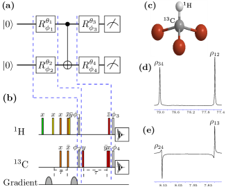
Figure 1: (Color online) (a) Quantum circuit to implement CS-QPT of a CNOT gate. Single-qubit unitary operations $R_{\phi}^{\theta}$ are achieved via rotations by an angle $\theta$ and phase $\phi$. The first block represents the preparation of the desired input state, while the second and third blocks represent the quantum process corresponding to the CNOT gate and the measurement, respectively. (b) NMR implementation of the quantum circuit given in panel (a). The rectangles filled with red, orange, yellow and green color denote $\frac{\pi}{2}$, $\pi$, $\frac{\pi}{4}$ and $\frac{\pi}{3}$ pulses, respectively, with the rf phase written above each pulse. The unfilled rectangles with the phases $\phi_{1}$, $\phi_{2}$, $\phi_{3}$, and $\phi_{4}$ represent pulses with flip angles $\theta_{1}$, $\theta_{2}$, $\theta_{3}$, and $\theta_{4}$, respectively. The gradient line denotes $z$-gradient pulses. The evolution time period $\tau=\frac{1}{2J_{CH}}$ where $J_{CH}$ is the scalar coupling constant. (c) ¹³C-labeled chloroform molecule with ¹H and ¹³C labeling the first and second qubits, respectively. (d) and (e) depict the NMR spectra of ¹³C and ¹H, respectively, corresponding to the configuration $\{|++\rangle\langle++|,IX\}$.

III Experimental implementation of CS-QPT

III.1 CS-QPT of two-qubit gates

We implemented the CS-QPT protocol for two, two-qubit nonlocal quantum gates, namely, the CNOT gate and the controlled-rotation gate. The controlled-rotation gate is a nonlocal gate which rotates the state of the second qubit via $R_{x}(\theta)$, if the first qubit is in the state $|1\rangle$.

For two qubits the tomographically complete set of input states is given by: $\{|0\rangle,|1\rangle,|+\rangle,|-\rangle\}^{\otimes 2}$ where $|+\rangle=(|0\rangle+|1\rangle)/\sqrt{2}$ and $|-\rangle=(|0\rangle+i|1\rangle)/\sqrt{2}$. In NMR, tomographic measurements are carried out by applying a set of unitary rotations followed by signal acquisitionLong et al. (2001). The time-domain NMR signal is recorded as a free induction decay and then Fourier transformed to obtain the frequency spectrum, which effectively measures the net magnetization in the transverse ($x-y$) plane. For two NMR qubits, the tomographically complete set of unitary rotations is given by Li et al. (2017): $\{II,IX,IY,XX\}$ where $II$ denotes the no operation on both the qubits, $IX$ denotes no operation on the first qubit and a $90^{\circ}$ $x$-rotation on the second qubit, $IY$ denotes no operation on the first qubit and a $90^{\circ}$ $y$-rotation on the second qubit and $XX$ denotes a $90^{\circ}$ $x$-rotation on both qubits.

As an illustration, the quantum circuit and corresponding NMR implementation of the CS-QPT protocol for a two-qubit CNOT gate is given in Fig. 1. Fig.1(a) depicts the general quantum circuit to acquire data for CS-QPT and contains all possible settings corresponding to a tomographically complete set of input quantum states and measurements. The first block in Fig.1(a) prepares the desired initial input state from $|00\rangle$. In the second block the quantum process (CNOT gate in this case) which is to be tomographed, is applied to the system qubits and in the third block, a set of tomographic operations are applied, followed by measurements on each qubit. To implement CS-QPT for any other two-qubit quantum gate, the CNOT gate should be replaced with the desired gate, while the remaining circuit remains unaltered. The first block in the Fig.1(b) represents the NMR pulse sequence which prepares the spin ensemble in the pseudo pure state (PPS) $|00\rangle$ and then generates the desired input state from the $|00\rangle$ state. The pulse sequence corresponding to the CNOT gate (the quantum process which is to be tomographed) is given in the second block and finally, in the last block, the desired set of tomographic pulses are applied and the NMR signal is acquired.

We used ${}^{13}C$-enriched chloroform molecule (Fig.1(c)) dissolved in acetone-D6 to physically realize a two-qubit system, with the ¹H and ¹³C spins denoting the first and second qubits, respectively. The NMR Hamiltonian in the rotating frame is given by:

$$\mathcal{H}=-\sum_{i=1}^{2}\nu_{i}I_{iz}+J_{\rm CH}I_{1z}I_{2z}$$ (7)

where $\nu_{1}$, $\nu_{2}$ are the chemical shifts, $I_{1z}$, $I_{2z}$ are the $z$-components of the spin angular momentum operators of the ¹H and ¹³C spins respectively, and $J_{{\rm CH}}$ is the scalar coupling constant. We used the spatial averaging technique to initialize the system in the PPS corresponding to $|00\rangle$, with the density matrix $\rho_{00}$ given by Oliveira et al. (2007):

$$\rho_{00}=\frac{1}{4}(1-\eta)I_{4}+\eta|00\rangle\langle 00|$$ (8)

where $\eta$ corresponds to the net spin magnetization at thermal equilibrium, and $I_{4}$ is a $4\times 4$ identity operator. Figs. 1(d) and 1(e) depict the NMR spectra corresponding to carbon and hydrogen respectively, obtained for the configuration $\{|++\rangle,IX\}$, where $\{|++\rangle$ refers to the initial state and $IX$ denotes the tomographic pulse set used. The system is prepared in the initial input state $|++\rangle$, a CNOT gate is applied, and finally the tomographic pulse $IX$ is applied to obtain the NMR spectrum. For the first qubit, the area under the spectrum is related to the density matrix elements $\rho_{24}$ and $\rho_{13}$, while for the second qubit, the area under the spectrum is related to the density matrix elements $\rho_{34}$ and $\rho_{12}$. In general, the four readout elements of the density matrix are complex numbers; in NMR the imaginary part of the density matrix can be calculated by applying a $90^{\circ}$ phase shift to the spectrum (post-processing) and then measuring the area Long et al. (2001). Hence a given configuration comprises four data points (two for each qubit). Since the size of the full configuration space is 64 (16 states $\times$ 4 tomographic rotations), the size of the full data set for two qubits is $64\times 4=256$. The vector $\overrightarrow{B}^{exp}_{\text{full}}$ (256$\times$1 dimensional) can be experimentally constructed by computing the area under the spectrum for the full configuration space. One can hence construct $\overrightarrow{B}^{exp}_{m}$ and the corresponding sub-matrix $\Phi_{m}$ by randomly selecting $m$ rows from $\overrightarrow{B}^{exp}_{\text{full}}$ and $\Phi_{\text{full}}$ respectively, solving the optimization problem (Eq. (5a)) for a reduced data set of size $m$, and estimating the process matrix; $m$ here refers to one particular configuration randomly chosen from the set of all possible 256 configurations.

III.2 CS-QPT of three-qubit gates

Figure 2: (Color online) Quantum circuit to implement CS-QPT of a Control-NOT-NOT ($U_{\rm{CNN}}$) gate. The first block prepares the desired input state while the second and third blocks represent the quantum process corresponding to the ($U_{\rm{CNN}}$) gate and the measurement, respectively. (b) NMR implementation of the quantum circuit given in panel (a). Solid black rectangles are refocusing pulses with flip angle $180^{\circ}$, while the gray rectangles represent pulses with flip angle $45^{\circ}$; the corresponding rf phases are written below each pulse. The value of $\beta$ is set to $60^{\circ}$, while the unfilled rectangles with rf phases $\phi_{1}$, $\phi_{2}$ and $\phi_{3}$ correspond to flip angles $\theta_{1}$, $\theta_{2}$ and $\theta_{3}$, respectively. The black rectangles represent pulses with flip angle $90^{\circ}$. The unfilled rectangles in the last block, of phases $\phi_{1}$, $\phi_{2}$ and $\phi_{3}$ correspond to flip angles $\theta_{1}$, $\theta_{2}$ and $\theta_{3}$, respectively which implement tomographic operations followed by measurement on each qubit; $\tau_{ij}=\frac{1}{2J_{ij}}$. (c) ${}^{13}C$-labeled diethyl fluoromalonate with ¹H, ¹⁹F and ¹³C nuclei labeled as the first, second and third qubits, respectively. NMR spectra depicted in (d), (e) and (f) correspond to ¹H, ¹⁹F and ¹³C nuclei respectively, for the configuration $\{|11+\rangle\langle 11+|,XYX\}$.

We have implemented the CS-QPT protocol to characterize the three-qubit controlled-NOT-NOT ($U_{{\rm CNN}}$) gate with multiple targets, with the first qubit being denoted the control qubit, while the other two qubits are the target qubits. The controlled-NOT-NOT gate can be decomposed using two CNOT gates as: $U_{{\rm CNN}}\equiv$ CNOT${}_{13}.$CNOT₁₂, and is widely used in encoding initial input states in error correction codes, fault tolerant operations Egan et al. (2021); Shor (1995) and in the preparation of three-qubit maximally entangled states Mooney et al. (2021); Singh et al. (2018); Dogra et al. (2015).

The NMR Hamiltonian for three qubits in the rotating frame is given by:

$$\mathcal{H}=-\sum_{i=1}^{3}\nu_{i}I_{iz}+\sum_{i,j=1(i\neq j)}^{3}J_{ij}I_{iz}I_{jz}$$ (9)

where the indices $i,j$ label the qubit and $\nu_{i}$ denotes the respective chemical shift. The quantity $J_{ij}$ denotes the scalar coupling strengths between the $i$th and $j$th qubits, while $I_{iz}$ represents the $z$-component of the spin angular momentum of the $i$th qubit. We have used ¹³C-labeled diethyl fluoromalonate (Fig.2(c)) dissolved in acetone-D6 to physically realize a three-qubit system, with the ¹H, ¹⁹F and ¹³C nuclei being labeled as the first, second and third qubits, respectively. State initialization is performed by preparing the system in the PPS $|000\rangle$ via the spatial averaging technique with the corresponding density matrix being given by:

$$\rho_{000}=(\frac{1-\epsilon}{8})I_{8}+\epsilon|000\rangle\langle 000|$$ (10)

where $\epsilon\approx 10^{-5}$ represents the net thermal magnetization and $I_{8}$ is the 8$\times$8 identity operator.

For a three-qubit system, the tomographically complete set of input states is given by: $\{|0\rangle,|1\rangle,|+\rangle,|-\rangle\}^{\otimes 3}$ where $|+\rangle=(|0\rangle+|1\rangle)/\sqrt{2}$ and $|-\rangle=(|0\rangle+i|1\rangle)/\sqrt{2}$ and the tomographically complete set of unitary rotations is given by: $\{III,IIY,IYY,YII,XYX,XXY,XXX\}$ Li et al. (2017). The quantum circuit and the corresponding NMR pulse sequence to perform CS-QPT for the three-qubit gate $U_{\rm CNN}$ is given in Fig. 2. The first block in Fig.2(a) represents the input state preparation while the second block represents the application of quantum gate $U_{\rm{CNN}}$ (i.e. quantum process which is to be tomographed), and tomographic unitary rotations are applied in the last block, followed by measurement on each qubit. Fig.2(b) represents the corresponding NMR implementation of quantum circuit given in the Fig.2(a). The spatial averaging techniques are used in the first block Singh et al. (2019) to initialize system in the desired PPS, followed by the application of spin-selective rf pulses to prepare the desired input state. In the second block the pulse sequence corresponding to $U_{\rm{CNN}}$ is applied on the input state and in the last block after application of tomographic pulses, the signal of the desired nucleus is recorded. The NMR spectra corresponding to ¹H, ¹⁹F and ¹³C are given in Figs. 2(d), (e) and (f), respectively, for the configuration $\{|11+\rangle\langle 11+|,XYX\}$, i.e. the input state $|11+\rangle\langle 11+|$ is prepared, evolved under the quantum process corresponding to $U_{\rm{CNN}}$, the tomographic set of pulses $XYX$ is applied, and finally the NMR signal is recorded. For the first qubit (¹H) the area under the four spectral lines correspond to the density matrix elements $\rho_{48}$, $\rho_{26}$, $\rho_{37}$ and $\rho_{15}$, for the second qubit (¹⁹F) the area under the four spectral lines correspond to the density matrix elements $\rho_{57}$, $\rho_{13}$, $\rho_{68}$ and $\rho_{24}$, while for the third qubit (¹³C), the area under the four spectral lines correspond to the density matrix elements $\rho_{56}$, $\rho_{12}$, $\rho_{78}$ and $\rho_{34}$, respectively. For a three-qubit system there are 12 experimental data points (4 per qubit) for a given configuration and the total number configurations are 448 (64 input states $\times$ 7 tomographic unitary operations) which yields the $\overrightarrow{B}^{exp}_{\text{full}}$ of size = 5376 (448 configurations $\times$ 12 data points per configuration). One can construct $\overrightarrow{B}^{exp}_{\text{m}}$ by randomly selecting $m$ number of rows from $\overrightarrow{B}^{exp}_{\text{full}}$, and using the corresponding coefficient matrix $\Phi_{m}$ one can solve the optimization problem (Eq. (5a)), and construct the process matrix for a reduced data set of size $m$.

III.3 CS-QPT of two-qubit processes in a three-qubit system

In order to experimentally implement a two-qubit CNOT gate in a multi-qubit system, one needs to allow the two system qubits to interact with each other i.e. , let them evolve under the internal coupling Hamiltonian for a finite time. In reality, this is non-trivial to achieve experimentally, as during the evolution time the other qubits are also continuously interacting with system qubits, and one has to “decouple” the system qubits from the other qubits. In the language of NMR, this is referred to as refocusing of the scalar $J$-coupling.

To implement a two-qubit CNOT gate we need four single-qubit rotation gates and one free evolution under the internal coupling Hamiltonian (Fig. 1). The single-qubit rotation gates are achieved by applying very short duration rf pulses of length $\approx 10^{-6}$ s, while the time required for free evolution under the coupling Hamiltonian is $\approx 10^{-3}$ s. The quality of the experimentally implemented quantum gate depends on the time required for gate implementation, which for the two-qubit CNOT gate, is primarily determined by the free evolution under the coupling Hamiltonian. We use the CS-QPT protocol to efficiently characterize three coupling evolutions corresponding to $U^{J}_{ij}$ of the form:

$$U^{J}_{ij}(t)=e^{-i2\pi J_{ij}I_{iz}I_{jz}t}$$ (11)

where the indices $i$ and $j$ label the qubits and $J_{ij}$ is the strength of the scalar coupling between the $i$th and the $j$th qubit; for the CNOT gate, $t=|\frac{1}{2J_{ij}}|$. A three-qubit system is continuously evolving under all the three $J_{ij}$ couplings, so in order to let a subsystem of two qubits effectively evolve under one of these couplings, we have to refocus all the other $J$-couplings. For example, consider the two-qubit subsystem of the $i$th and $j$th qubit with the effective evolution $U_{ij}^{J}(t)$ given by:

$$U_{ij}^{J}(t)=U_{\rm{int}}(\frac{t}{2})R_{x}^{k}(\pi)U_{\rm{int}}(\frac{t}{2})R_{x}^{k}(-\pi)$$ (12)

where $R_{x}^{k}(\pm\pi)$ is an $x$-rotation on the $k$th qubit by an angle $\pm\pi$ and $U_{{\rm int}}(\frac{t}{2})$ is the unitary operator corresponding to free evolution for a duration $\frac{t}{2}$ under the internal Hamiltonian $\mathcal{H}_{{\rm int}}=\sum_{i,j=1,i>j}^{3}J_{ij}I_{iz}I_{jz}$. The procedure for tomographic reconstruction of the reduced two-qubit density matrix from the full three-qubit density matrix is given in Table. 1. We were able to successfully characterize all three $U_{ij}^{J}(t)$ via the CS-QPT method and constructed the corresponding process matrices, using a heavily reduced data set of size $\approx 20$, with experimental fidelities $>0.94$. Using the information given in Table 1, one can efficiently characterize a general quantum state as well as the dynamics of a two-qubit subsystem in a three-qubit system, wherein the experimental data is acquired by measuring only the two qubits under consideration; hence the complete set of input states and tomographic rotations required are the same as for the two-qubit protocol described in Section III.1.

Table 1: Relation between the readout positions of the reduced density matrix of the subsystem ($\rho_{ij}^{\prime}$) and the readout positions $\rho_{mn}$.

Subsystem	Readout positions of the reduced density matrix
	$\rho_{24}^{\prime}$	$\rho_{13}^{\prime}$	$\rho_{34}^{\prime}$	$\rho_{12}^{\prime}$
1H+19F	$\rho_{48}+\rho_{37}$	$\rho_{26}+\rho_{15}$	$\rho_{57}+\rho_{68}$	$\rho_{13}+\rho_{24}$
1H+13C	$\rho_{48}+\rho_{26}$	$\rho_{37}+\rho_{15}$	$\rho_{56}+\rho_{78}$	$\rho_{12}+\rho_{34}$
19F+13C	$\rho_{68}+\rho_{24}$	$\rho_{57}+\rho_{13}$	$\rho_{78}+\rho_{34}$	$\rho_{56}+\rho_{12}$

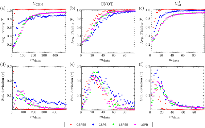
Figure 3: (Color online) The top panel represents the average gate fidelity $\overline{\mathcal{F}}$ corresponding to (a) a three-qubit $U_{\rm{CNN}}$ gate, (b) a CNOT gate and (c) $U^{J}_{23}$ against the number of data points $m_{\text{data}}$ on the $x$-axis. The bottom panel represents the standard deviation in average fidelity $\sigma$, corresponding to (d) a three-qubit $U_{\rm{CNN}}$ gate, (e) a CNOT gate, and (f) $U^{J}_{23}$, plotted against the number of data points $m_{\text{data}}$ on the $x$-axis. The data points in red, blue, green and pink correspond to CS-PEB, CS-PB, LS-PEB and LS-PB methods, respectively. The CS-PEB method shows the best performance for all three quantum gates.

Table 2: The minimum value of $m_{\rm{data}}$ at which the experimental average gate fidelity $\overline{\mathcal{F}}$ turns to be $>0.9$ is computed (alongwith the standard deviation $\sigma$) for different quantum processes, via the CS-PEB, CS-PB, LS-PEB and LS-PB methods.

	CS-PEB			CS-PB			LS-PEB			LS-PB
Gate	$m_{\rm{data}}$	$\overline{\mathcal{F}}$	$\sigma$	$m_{\rm{data}}$	$\overline{\mathcal{F}}$	$\sigma$	$m_{\rm{data}}$	$\overline{\mathcal{F}}$	$\sigma$	$m_{\rm{data}}$	$\overline{\mathcal{F}}$	$\sigma$
$U_{\rm{CNN}}$	30	0.9920	0.0081	-	-	-	320	0.9109	0.0123	290	0.9006	0.0147
CNOT	44	0.9798	0.0701	62	0.9203	0.0905	52	0.9514	0.0263	48	0.9308	0.0475
C-$R_{x}^{\pi}$	48	0.9728	0.0797	58	0.9068	0.0746	48	0.9332	0.0805	52	0.9503	0.0504
$U^{J}_{12}$	14	0.9549	0.0963	24	0.9464	0.0468	32	0.9075	0.0459	34	0.9071	0.0561
$U^{J}_{23}$	14	0.9641	0.0734	28	0.9145	0.0710	66	0.9019	0.0217	68	0.9048	0.0198
$U^{J}_{13}$	18	0.9417	0.0980	38	0.9067	0.0695	-	-	-	-	-	-

III.4 Comparison of CS-QPT and LS-QPT protocols

Table 3: Experimental quantum process fidelities obtained via CS and LS methods using the full data set $m^{\rm{full}}_{\rm{data}}$.

Gate	CS-PEB	CS-PB	LS-PEB	LS-PB
$U_{\rm{CNN}}$	0.9980	0.8877	0.9542	0.9542
CNOT	0.9984	0.9843	0.9817	0.9817
C-$R^{\pi}_{x}$	0.9980	0.9744	0.9831	0.9831
$U^{J}_{12}$	0.9967	0.9894	0.9819	0.9819
$U^{J}_{23}$	0.9976	0.9793	0.9273	0.9273
$U^{J}_{13}$	0.9895	0.9710	0.8942	0.8942

The fidelity of the experimentally estimated $\chi_{{\rm exp}}$ is computed using the measureZhang et al. (2014):

$${\mathcal{F}}(\chi_{\rm exp},\chi_{\rm ideal})=\frac{|{\rm Tr}[\chi_{\rm exp}\chi_{\rm ideal}^{\dagger}]|}{\sqrt{{\rm Tr}[\chi_{\rm exp}^{\dagger}\chi_{\rm exp}]{\rm Tr}[\chi_{\rm ideal}^{\dagger}\chi_{\rm ideal}]}}$$ (13)

where $\chi_{\text{ideal}}$ is the theoretically constructed process matrix, and as $\chi_{\rm{exp}}\rightarrow\chi_{\rm{ideal}}$, ${\mathcal{F}}(\chi_{\rm exp},\chi_{\rm ideal})\rightarrow 1$.

We performed QPT of several two- and three-qubit quantum gates using both CS-QPT and LS-QPT protocols on a reduced data set. The CS-QPT method was implemented for the PEB and PB basis sets. For a two-qubit system $m_{\text{data}}^{\rm full}=256$, while for a three-qubit system, $m_{\text{data}}^{\rm full}=5376$, where $m_{\text{data}}^{\rm full}$ denotes the size of the full data set obtained using the complete set of input states and tomographic rotation operators for two and three qubits as given in Sections III.1 and III.2, respectively. In the PEB basis, $\chi_{\text{ideal}}$ is maximally sparse for all unitary quantum gates, while in the PB basis, $\chi_{\text{ideal}}$ corresponding to the two-qubit CNOT, controlled-$R_{x}^{\pi}$ and $U^{J}_{ij}$ gates have 16, 16 and 4 non-zero elements, respectively (out of a total of 256 elements). For the three-qubit gate $U_{\rm CNN}$, $\chi_{\text{ideal}}$ has 16 non-zero elements (out of a total of 4096 elements).

The performance of the CS-QPT method was compared with the LS-QPT method for six different quantum processes corresponding to: (i) a three-qubit $U_{\rm CNN}$ gate, (ii) a two-qubit CNOT gate, (iii) a controlled-$R_{x}^{\pi}$ rotation (iv) $U^{J}_{23}$, (v) $U^{J}_{13}$ and (vi) $U^{J}_{12}$, of which the results of the quantum process corresponding to (a) a three-qubit $U_{\rm CNN}$ gate, (b) a two-qubit CNOT gate and (c) $U^{J}_{23}$, are displayed in Fig. 3. The top panel in Fig. 3 represents the average gate fidelity $\overline{\mathcal{F}}$ plotted against $m_{\text{data}}$, while the bottom panel represents the standard deviation $\sigma$ in average gate fidelity plotted against $m_{\text{data}}$. The average gate fidelity is obtained using the average process matrix estimated via the LS and CS algorithm in the PEB and PB bases. The plots in red and blue color represent the results of the CS-QPT method implemented in PEB and PB basis respectively, while the plots in green and pink color represent the results of the LS-QPT method implemented in the PEB and PB basis, respectively. The average fidelity and the value of $\sigma$ is computed by implementing the CS-QPT and LS-QPT protocols 50 times for randomly selected $m_{\text{data}}$ number of data points, and $\sigma$ is calculated from:

$$\sigma=\sqrt{\frac{\sum_{i=1}^{N}(\mathcal{F}_{i}-\overline{\mathcal{F}})^{2}}{N-1}}$$ (14)

where $N=50$ and $\overline{\mathcal{F}}$ is the average fidelity.

The plots in the first column of Fig. 3 correspond to the three-qubit gate $U_{\rm{CNN}}$, where Fig. 3(a) depicts the accuracy, while Fig. 3(d) gives the precision in characterizing $U_{\rm{CNN}}$, for a given value of $m_{\text{data}}$. Similarly, the second and third columns in Fig. 3 represent the experimental results corresponding to the CNOT gate and the $U^{J}_{23}$ quantum process, respectively. The plots corresponding to the two-qubit controlled-rotation gate (C-R${}_{x}^{\pi}$) is similar to the CNOT gate, while the plots corresponding to $U^{J}_{13}$ and $U^{J}_{12}$ are similar to $U^{J}_{23}$ (plots not shown). As seen from Fig. 3, the CS-QPT method implemented in the PEB basis, performs significantly better than the LS-QPT and the CS-QPT methods implemented in the PB basis, for all the quantum processes considered. The performance of the LS-QPT method is independent of the choice of basis operators. On the other hand, the CS-QPT method may yield a lower fidelity as compared to the LS-QPT method, if the basis operators are not properly chosen. Using a reduced data set, the overall performance for the three-qubit gate $U_{\rm{CNN}}$ is CS-PEB $>$ CS-PB $>$ LS-PEB $\approx$ LS-PB, while for the two-qubit CNOT and C-R${}_{x}^{\pi}$ gates, CS-PEB $>$ LS-PEB$\approx$ LS-PB $>$ CS-PB. For the two-qubit $U_{ij}^{J}$ processes, CS-PEB $>$ CS-PB $>$ LS-PEB $\approx$ LS-PB.

For the two-qubit CNOT and C-R${}_{x}^{\pi}$ gates, the LS algorithm performs better than the CS algorithm in the PB basis for all values of $m_{\rm{data}}$, while for the three-qubit $U_{\rm{CNN}}$ gate, the LS algorithm performs better than the CS algorithm in the PB basis for $m_{\rm{data}}\geq 160$, which clearly shows the importance of selecting an appropriate operator basis set while implementing the CS algorithm. The plots given in Fig. 3 provide information about the experimental complexity of the CS and LS algorithms i.e. the number of experiments required in each case to characterize a given quantum process. We note here in passing that the standard deviation in average fidelity ($\sigma$) is not monotonic. For small values of $m_{\rm{data}}$, the process of randomly selecting $m_{\rm{data}}$ data points to estimate the process matrix is more likely to lead to a lower fidelity and higher values of the standard deviation $\sigma$, and hence lower precision. For the two-qubit CNOT and controlled-R${}_{x}^{\pi}$ gates, $\sigma$ has a maximum around $m_{\rm{data}}\approx 20$, while for the $U_{CNN}$, $U^{J}_{23}$, $U^{J}_{13}$ and $U^{J}_{12}$ quantum processes, $\sigma$ is maximum around $m_{\rm{data}}\approx 10$. For all the cases, the CS-PEB method yields better precision as compared to the CS-PB, LS-PEB and LS-PB methods.

The experimentally obtained minimum value of $m_{\rm{data}}$ at which the experimentally computed average gate fidelity is $>0.9$ is given in Table 2, for all the quantum processes. For the three-qubit $U_{\rm{CNN}}$ gate, we experimentally obtained $\overline{\mathcal{F}}_{\rm{CS-PEB}}=0.9920\pm 0.0081$ for a reduced data set of size $m_{\rm{data}}=30$. For the two-qubit CNOT and control-$R_{x}^{\pi}$ gates, $\overline{\mathcal{F}}_{\rm{CS-PEB}}\geq 0.9790\pm 0.0701$ and $\overline{\mathcal{F}}_{\rm{CS-PEB}}\geq 0.9729\pm 0.0797$ for $m_{\rm{data}}\geq 44$ and $m_{\rm{data}}\geq 48$, respectively. The reduced data set is $\approx 5$ times smaller than the full data set, which implies that the experimental complexity is reduced by $\approx 80\%$ as compared to the standard QPT method. Furthermore, for all the two-qubit quantum processes corresponding to $U_{ij}^{J}$, $\overline{\mathcal{F}}_{\rm{CS-PEB}}\geq 0.9417\pm 0.0980$ for $m_{\rm{data}}\geq 18$. This reduced data set is $\approx 12$ times smaller than the full data set which implies that the experimental complexity in these cases is reduced by $\approx 92\%$ as compared to the standard QPT method.

IV Concluding Remarks

We designed a general quantum circuit to acquire experimental data compatible with the CS-QPT algorithm. The proposed quantum circuit can also be used for other experimental platforms and can be extended to higher-dimensional systems. We successfully demonstrated the efficacy of the CS-QPT protocol for various quantum processes corresponding to the three-qubit $U_{\rm{CNN}}$ gate, two-qubit CNOT and controlled-rotation gates and several two-qubit $U_{ij}^{J}$ unitary operations. Our experimental comparison of the CS-QPT and LS-QPT schemes demonstrate that the CS-QPT protocol is far more efficient, provided that the process matrix is maximally sparse and that an appropriate operator basis is chosen.

Standard QPT protocols do not have access to prior information about the intended target unitary and hence require a large number of parameters to completely characterize the unknown quantum process. CS methods can be used to dramatically reduce the resources required to reliably estimate the full quantum process, in cases where there is substantial prior information available about the quantum process to be characterized. Since the CS-QPT method is uses fewer resource and is experimentally viable, it can be used to characterize higher-dimensional quantum gates and to validate the performance of large-scale quantum devices.