Freezing out critical fluctuations

Abstract:

We introduce a novel freeze-out procedure connecting the hydrodynamic evolution of a droplet of quark-gluon plasma (QGP) that has, as it expanded and cooled, passed close to a posited critical point on the QCD phase diagram with the subsequent kinetic description in terms of observable hadrons. The procedure converts out-of-equilibrium critical fluctuations described by extended hydrodynamics, known as Hydro+, into cumulants of hadron multiplicities that can be subsequently measured. We introduce a critical sigma field whose fluctuations cause correlations between observed hadrons due to the couplings of the sigma field to the hadrons. We match the QGP fluctuations obtained via solving the Hydro+ equations describing the evolution of critical fluctuations before freeze-out to the correlations of the sigma field. In turn, these are imprinted onto fluctuations in the multiplicities of hadrons, most importantly protons, after freeze-out via a generalization of the familiar half-a-century-old Cooper-Frye freeze-out prescription [2] which we introduce [3]. This framework allows us to study the effects of critical slowing down and the consequent deviation of the observable predictions from equilibrium expectations quantitatively. We can also quantify the suppression of cumulants due to conservation of baryon number. We demonstrate the prescription in practice by freezing out the Hydro+ simulation in a simplified azimuthally symmetric and boost invariant background discussed in Ref. [4].

1 Introduction

A simulation of heavy-ion collisions is a multi-stage process involving initial state dynamics, hydrodynamic evolution and a hadronic afterburner. Transitions between subsequent stages involve matching and translating dynamical variables used at one stage into those used at the next stage in a way consistent with physics laws. In this work, we discuss the transition between the hydrodynamic stage and the hadronic stage, for the special case of heavy-ion collisions that produce a droplet of matter whose hydrodynamic evolution occurs in the vicinity of a critical point on the phase diagram of QCD. Traditionally, the macroscopic description of the quark gluon plasma in terms of the hydrodynamic variables is translated into a simplified hadronic description in terms of kinetic variables of an expanding ideal resonance gas of hadrons via the well-known Cooper-Frye procedure [2]. The Cooper-Frye freeze-out procedure has been successfully employed in the description of high energy heavy-ion collision data for almost 50 years. The procedure ensures that the event averaged charge and energy-momentum densities are matched between the two descriptions. At sufficiently high collision energies $\sqrt{s}$, the data from many experiments are in reasonable agreement with this description across a broad kinematic regime.

The Cooper-Frye framework, however, does not describe fluctuations. Such a description is crucial in the special case of heavy ion collisions that freeze out in the vicinity of a critical point. In this case fluctuations are both enhanced and of considerable interest, since it is via detecting critical fluctuations that we hope to discern the presence of a critical point [5, 6]. The deviations of certain measures of fluctuations from their non-critical baseline measured in Phase I of the Beam Energy Scan at RHIC, deviations that vary non-monotonically as a function of $\sqrt{s}$, provide intriguing hints for the possible existence of a critical point in the QCD phase diagram [7, 8]. To convert these hints into definitive conclusions and thereby potentially discover the location of the critical point, one needs theoretical modeling that provides guidance as to what to expect in this case. Much work is being done by a number of groups to develop a description of the hydrodynamics with critical fluctuations near a critical point [9, 10]. In addition to such a description, we need a freeze-out procedure to translate not only average hydrodynamic variables but also the critical fluctuations exhibited by the quark gluon plasma into the mean and fluctuations of hadron multiplicities that are subsequently observed. This is the goal of this work.

Since the correlation length, $\xi$, grows near the critical point, the typical relaxation time for local thermodynamic equilibration increases. This is commonly referred to as critical slowing down. There is a competition between the local relaxation rate and the hydrodynamic evolution rate. As the hydrodynamic fields evolve, if relaxation rates are slow, as is the case for fluctuations near a critical point, these fluctuations can no longer be described by their equilibrium values slaved to hydrodynamic fields. There has been a considerable amount of work performed within both the stochastic and deterministic approaches to describe the evolution of fluctuations near the critical point [9, 10]. In the deterministic approach, the correlation functions that describe the fluctuations, in essence, their moments, are considered as additional degrees of freedom with evolution equations of their own. In this work, we introduce a prescription to convert these fluctuations, so described, into correlations of observed particles. The results shown here are based on work in progress [3].

2 Extended Cooper-Frye freeze-out near a critical point

To describe the critical fluctuations on the kinetic side, after freeze-out, the particle distribution function has to be modified from an ideal gas of hadrons to one in which the correlations anticipated near the QCD critical point are manifest. While there could be many ways of doing this, in our work we choose to incorporate the critical fluctuations via the interaction of the particle fields with a critical $\sigma$ field that controls the masses of hadrons. The model that we describe here has been discussed in equilibrium settings and also in non-equilibrium settings in the past [11, 12]. In this work, we first match the correlations of the $\sigma$ field to hydrodynamic fluctuations. The masses of particles at freeze-out then depend on the background field $\sigma$. We denote $g_{A}$ as the coupling between the $\sigma$ field and the field corresponding to the particle species $A$. Small deviations of $\sigma$ from its equilibrium value change the mass of particle $A$, to leading order as

$$\delta m_{A}=g_{A}\sigma$$ (1)

and the modified distribution function is

$$f_{A}=\left<f_{A}\right>+g_{A}\frac{\partial\left<f_{A}\right>}{\partial m_{A}}\sigma\ .$$ (2)

In Eq. (2), $\left<f_{A}\right>$ is the particle distribution function for an ideal gas. We ignore quantum statistics and viscous corrections and use the Boltzmann distribution function $\left<f_{A}\right>=\exp\left\{-\frac{p\cdot u}{T}+\frac{\mu_{A}}{T}\right\}$. We define $\sigma$ so that $\left<\sigma\right>\equiv 0$. Hence, the mean multiplicity of particle species $A$ denoted by $\left<N_{A}\right>$ is left unchanged from the Cooper-Frye prescription [2]:

$$\left<N_{A}\right> = d_{A}\int dS_{\mu}\,\int Dp_{A}\,p^{\mu}\,\left<f_{A}(x,p)\right>\ .$$ (3)

where $d_{A}$ is the (iso)spin degeneracy of the particle $A$. In Eq. (3), $dS_{\mu}$ is a differential element on the freeze-out hypersurface pointing along the normal and $Dp_{A}$ is given by

$$Dp_{A}=2\frac{d^{4}p}{(2\pi)^{3}}\delta\left(p^{2}-m_{A}^{2}\right)\theta(p^{0})\ .$$ (4)

The two-point correlation function $\left<\sigma(x_{+})\sigma(x_{-})\right>$ is proportional to the two-point correlation function of the slowest mode, namely fluctuations of entropy per baryon, denoted by $\hat{s}\equiv s/n$:

$$\left<\sigma(x_{1})\sigma(x_{2})\right> = Z(x)\,\left<\delta\hat{s}(x_{1})\delta\hat{s}(x_{2})\right>\ .$$ (5)

Here, $Z$ is a function of thermodynamic fields which depends on the QCD equation of state near the critical point. In this work, we focus on matching the leading singular contribution to the two-point correlation function between the hydrodynamic and kinetic descriptions. With Eq. (5), the critical contribution to the variance of the multiplicity of particles of species $A$ is then given by

$$\left<\delta N_{A}^{2}\right>_{\sigma} = g_{A}^{2}\,\int dS_{\mu,+}\,\int dS_{\nu,-}\,Z(x)\,J_{A}^{\mu}(x_{+})\,J_{A}^{\nu}(x_{-})\,\left<\delta\hat{s}(x_{+})\delta\hat{s}(x_{-})\right>\ ,$$ (6)

where

$$J_{A}^{\alpha}(x_{\pm}) \equiv \frac{d_{A}m_{A}}{T(x_{\pm})}\int\,Dp_{A}\,\frac{\partial\left<f_{A}(x,p)\right>}{\partial m_{A}}\,p^{\alpha}\ .$$ (7)

The total variance of the multiplicity of $A$ particles is the Poisson value plus the critical part, namely $\left<\delta N_{A}^{2}\right>=\left<N_{A}\right>+\left<\delta N_{A}^{2}\right>_{\sigma}$.

3 Demonstration in an azimuthally symmetric boost invariant Hydro+ simulation

The Hydro+ framework combining hydrodynamics with a deterministic description of out-of-equilibrium critical fluctuations was introduced in Ref. [13]. We shall use the prescription introduced in the previous Section to freeze out a Hydro+ simulation discussed in Ref. [4]. The correlation function of $\hat{s}\equiv s/n$ can be expressed in terms of its Wigner transform:

$$\phi_{\bm{Q}}(x)=\int_{\Delta x}\left<\delta\hat{s}\left(x_{+}\right)\delta\hat{s}\left(x_{-}\right)\right>\,e^{iQ\cdot\Delta x}\ .$$ (8)

Here $x=(x_{+}+x_{-})/2$ and $\Delta x=x_{+}-x_{-}$ and the integral is performed over an equal-time hypersurface in the local rest frame at $x$. The relaxation of this quantity to its local equilibrium value $\bar{\phi}_{\bm{Q}}$ is governed by the equation [13]:

$$u(x)\cdot\partial\phi_{\bm{Q}}(x)=-\Gamma(\bm{Q})\,\left(\phi_{\bm{Q}}(x)-\bar{\phi}_{\bm{Q}}(x)\right)\ ,$$ (9)

where $\bar{\phi}_{\mathbf{Q}}$ can be adequately approximated by the Ornstein-Zernike ansatz as in Ref. [4]:

$$\bar{\phi}_{\bm{Q}}\approx\frac{c_{M}\xi^{2}}{1+(Q\xi)^{2}}\ .$$ (10)

The leading behavior of the $Q$-dependent relaxation rate $\Gamma$ near a critical point with Model H relaxation dynamics is given by:

$$\Gamma(\bm{Q})=\frac{2D_{0}\xi_{0}}{\xi^{3}}K(Q\xi)\ ,$$ (11)

where $K(x)=\frac{3}{4}\left[1+x^{2}+(x^{3}-x^{-1})\arctan x\right]$. Because $\phi_{\bm{Q}}$ describes fluctuations of the diffusive mode $\hat{s}$, the rate vanishes at $\bm{Q}=0$, i.e., $\Gamma\approx 2DQ^{2}$ where $D=D_{0}\xi_{0}/\xi$ is the diffusion coefficient, also vanishing at the critical point.

We evolve the $\phi_{\bm{Q}}$’s according to Eq. (9) in an azimuthally symmetric and boost invariant background using the code described in Ref. [4]. As the trajectory on the phase diagram describing the history of a given fluid cell passes by the critical point, the equilibrium correlation length $\xi$ increases to a maximum value $\xi_{\rm max}$ before falling back to its value at freezeout. We shall use variable $\xi_{\rm max}$ to describe the effect of varying the $\sqrt{s}$ of the collision on how close the trajectory passes to the critical point. We use the parametrization for the correlation length $\xi$ as a function of the decreasing temperature $T$ along the trajectory from Ref. [4]:

$$\left(\frac{\xi}{\xi_{0}}\right)^{-4}=\tanh^{2}\left(\frac{T-T_{c}}{\Delta T}\right)\left[1-\left(\frac{\xi_{\text{max}}}{\xi_{0}}\right)^{-4}\right]+\left(\frac{\xi_{\text{max}}}{\xi_{0}}\right)^{-4}\ .$$ (12)

In Eq. (12), $T_{c}$ is the (crossover) temperature at the point along the system’s trajectory that is closest to the critical point and $\Delta T$ sets the size of the critical region. $\xi_{0}$ is the non-critical correlation length away from the critical point. We set the parameters in Eq. (12) to $\xi_{0}=0.5\,\text{fm}$, $T_{c}=0.16\,\text{GeV}$, and $\Delta T=0.2\,T_{c}$.

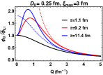
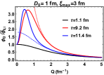
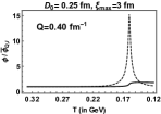
Figure 1: Normalized $\phi_{\bm{Q}}$’s as a function of $Q\equiv|\mathbf{Q}|$ in a fluid cell near the center of the fireball are shown in the first and second plots from the left for $D_{0}$ values of $0.25\,\text{fm}$ and $1\,\text{fm}$ respectively. The thick and dashed black curves in the these plots are the normalized $\phi_{\bm{Q}}$ and $\bar{\phi}_{\bm{Q}}$ at the corresponding proper time $\tau$ values, where $\bar{\phi}_{\bm{Q}}$ denotes the value that $\phi_{\bm{Q}}$ would have if it were in equilibrium. The normalization factor $\bar{\phi}_{\bm{Q}}\equiv\bar{\phi}_{\bm{Q}}(T(\tau_{I}))$. The temperatures at different times are $T(9.2\mbox{ fm})=0.14\mbox{ GeV}$ and $T(11.4\mbox{ fm})=0.16\mbox{ GeV}$. The third and fourth plots from the left show the normalized $\phi_{\bm{Q}}$ and $\bar{\phi}_{\bm{Q}}$ as functions of the temperature (i.e., of time) for $Q=0.4\,\text{fm}^{-1}$.

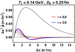
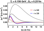
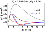
Figure 2: Position-space correlator of $s/n$ fluctuations $\tilde{\phi}$: Here, we plot $\Delta x^{2}\tilde{\phi}$, as a function of the spatial separation $\Delta x$ between the points. We plot results on two different isothermal freeze-out hypersurfaces ($T=0.14$ and $0.156$ GeV) for two values of $D_{0}$’s at two radial coordinates. The dashed black curve is the equilibrium correlator at freeze-out. The dashed brown curve is the equilibrium correlator far from the critical point, i.e., when $\xi=\xi_{0}$. The dotted black curve is the equilibrium correlator at $T=T_{c}$.

The $\phi_{\mathbf{Q}}$’s at various points along the trajectory of a fluid cell near the center of the fireball (radial position $r=0.7\,\text{fm}$ at initial proper time $\tau_{I}=1.1\,\text{fm}$) are shown in Fig. 1 for two relaxation rates (11) characterized by differing values of the parameter $D_{0}$ which specifies the diffusion constant. The curves in Fig. 1 do not evolve at $\bm{Q}=0$ because the conservation of baryon number dictates the diffusive nature of the $\hat{s}$ mode, which is a function of $n$, and its fluctuations $\phi_{\bm{Q}}$. Upon increasing the $D_{0}$ value from 0.25 fm to 1 fm, we see an enhancement in fluctuations as they relax faster to their large equilibrium values near the critical point. In this work, we considered two isothermal freeze-out scenarios namely $T_{f}=0.14\,\text{GeV}$ and $T_{f}=0.156\,\text{GeV}$. The inverse Wigner transform, i.e., the coordinate space correlation function $\tilde{\phi}(\Delta x,x)\equiv\left<\delta\hat{s}(x_{+})\delta\hat{s}(x_{-})\right>$, is plotted for $D_{0}$ equal to 0.25 fm and 1 fm on each of these freezeout surfaces in Fig. 2.

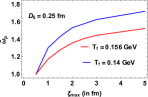
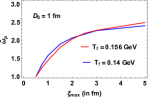
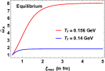
Figure 3: Normalized fluctuation measure $\tilde{\omega}_{A}$ (defined in Eq. (14)) as a function of $\xi_{\text{max}}$ which is the maximum equilibrium correlation length reached during the hydrodynamic evolution. As $D_{0}\rightarrow\infty$, the $\tilde{\omega}_{A}$’s approach their equilibrium values .

We denote the ratio of the variance defined in Eq. (6) to the mean multiplicity defined in Eq. (3) by $\omega_{A}$:

$$\omega_{A}\equiv\frac{\left<\delta N_{A}^{2}\right>_{\sigma}}{\left<N_{A}\right>}\ .$$ (13)

The excess of the critical fluctuations over the non-critical baseline $\omega_{A}^{\text{nc}}$ can be quantified via the ratio

$$\tilde{\omega}_{A}\equiv\frac{\omega_{A}}{\omega_{A}^{\text{nc}}}\ ,$$ (14)

where $\omega_{A}^{\text{nc}}$ is our estimate for the value of $\omega_{A}$ when the correlation length is not enhanced due to proximity to a critical point, namely when it is equal to the non-critical value $\xi_{0}$. $\tilde{\omega}_{A}$ for protons obtained within the Hydro+ framework for the simulation from Ref. [4] is shown in Fig. 3.

4 Discussions and Outlook

In this work, we have introduced an extended Cooper-Frye procedure to freeze out critical fluctuations. We have also implemented it in freezing out a simplified Hydro+ simulation in an azimuthally symmetric and boost invariant background. We observe that due to critical slowing down, the out-of-equilibrium fluctuations did not grow as large near the critical point as they would have if they were able to stay in equilibrium. Helpfully, though, and again due to critical slowing down, we find the fluctuations to be less sensitive to how much lower the freeze-out temperature is than the temperature of the critical point itself than would be the case in equilibrium. This can be seen by comparing the first three panels from the left in Fig. (3) to the right-most panel.

The estimates that we have made in this exploratory study have relied upon many simplifications. They can be made more quantitative by employing more realistic scenarios with more appropriate initial state dynamics, a more realistic equation of state, effects of baryon stopping, and a hadronic afterburner. The coupling constant $g_{A}$, which sets the magnitude of the fluctuations, is not well known. However, one could constrain it by comparing the equation of state of QCD to the equation of state of a hadron resonance gas model. We have also ignored the sub-leading singularities near the critical point and the background terms in the evolution equation for the two-point correlation function. Relaxing these assumptions would be another way to improve the estimates we have presented here. The procedure also remains to be applied to obtain correlations of particles other than protons and pions in the hadron resonance gas model.

All that said, we see it as of paramount importance to extend the application of this procedure to higher-order non-Gauusian cumulants, as they serve as stronger signals of the critical point [14, 12]. While this will be the next immediate step to do, we also hope that the procedure we have developed and presented here can already be implemented within the full paradigm for the numerical simulation of beam energy scan at RHIC [10].

5 Acknowledgement

We gratefully acknowledge the contributions of Ryan Weller, who collaborated with us on this research project during its early stages. This work was supported by the U.S. Department of Energy, Office of Science, Office of Nuclear Physics, within the framework of the Beam Energy Scan Theory (BEST) Topical Collaboration and grants DE-SC0011090 and DE-FG0201ER41195. Y.Y. acknowledges support from the Strategic Priority Research Program of the Chinese Academy of Sciences, Grant No. XDB34000000.

References

- [1]
- [2] F. Cooper and G. Frye, Phys. Rev. D 10, 186 (1974)
- [3] M. S. Pradeep, K. Rajagopal, M. Stephanov and Y. Yin (in preparation)
- [4] K. Rajagopal, G. Ridgway, R. Weller and Y. Yin, Phys. Rev. D 102, no.9, 094025 (2020) [arXiv:1908.08539 [hep-ph]]
- [5] M. A. Stephanov, K. Rajagopal and E. V. Shuryak, Phys. Rev. Lett. 81, 4816-4819 (1998) [arXiv:hep-ph/9806219 [hep-ph]].
- [6] M. A. Stephanov, K. Rajagopal and E. V. Shuryak, Phys. Rev. D 60, 114028 (1999) [arXiv:hep-ph/9903292 [hep-ph]].
- [7] A. Aprahamian, A. Robert, H. Caines, G. Cates, J. A. Cizewski, V. Cirigliano, D. J. Dean, A. Deshpande, R. Ent, et al. “Reaching for the horizon: The 2015 long range plan for nuclear science,” science.energy.gov/ ~/media/np/nsac/pdf/2015LRP/2015_LRPNS_091815.pdf, 2015.
- [8] M. Abdallah et al. [STAR Collaboration], Phys. Rev. C 104, no.2, 024902 (2021) [arXiv:2101.12413 [nucl-ex]].
- [9] M. Bluhm, A. Kalweit, M. Nahrgang, M. Arslandok, P. Braun-Munzinger, S. Floerchinger, E. S. Fraga, M. Gazdzicki, C. Hartnack, C. Herold, et al. Nucl. Phys. A 1003, 122016 (2020) [arXiv:2001.08831 [nucl-th]].
- [10] X. An, M. Bluhm, L. Du, G. V. Dunne, C. Gale, J. Grefa, U. Heinz, A. Huang, J. M. Karthein, D. E. Kharzeev, et al. [arXiv:2108.13867 [nucl-th]].
- [11] M. A. Stephanov, Phys. Rev. D 81, 054012 (2010) [arXiv:0911.1772 [hep-ph]].
- [12] C. Athanasiou, K. Rajagopal and M. Stephanov, Phys. Rev. D 82, 074008 (2010) [arXiv:1006.4636 [hep-ph]].
- [13] M. Stephanov and Y. Yin, Phys. Rev. D 98, no.3, 036006 (2018) [arXiv:1712.10305 [nucl-th]].
- [14] M. A. Stephanov, Phys. Rev. Lett. 102, 032301 (2009) [arXiv:0809.3450 [hep-ph]].