Free Surface in 2D Potential Flow: Singularities, Invariants and Virtual Fluid

Abstract

We study a 2D potential flow of an ideal fluid with a free surface with decaying conditions at infinity. By using the conformal variables approach, we study a particular solution of Euler equations having a pair of square–root branch points in the conformal plane, and find that the analytic continuation of the fluid complex potential and conformal map define a flow in the entire complex plane, excluding a vertical cut between the branch points. The expanded domain is called the “virtual” fluid, and it contains a vortex sheet whose dynamics is equivalent to the equations of motion posed at the free surface. The equations of fluid motion are analytically continued to both sides of the vertical branch cut (the vortex sheet), and additional time–invariants associated with the topology of conformal plane and Kelvin’s theorem for virtual fluid are explored. We called them “winding” and virtual circulation. This result can be generalized to a system of many cuts connecting many branch points, and resulting in a pair of invariants for each pair of branch points. We develop an asymptotic theory that shows how a solution originating from a single vertical cut forms a singularity at the free surface in infinite time, the rate of singularity approach is double-exponential, and supercedes the previous result of the short branch cut theory with finite time singularity formation.

The present work offers a new look at fluid dynamics with free surface by unifying the problem of motion of vortex sheets, and the problem of 2D water waves. A particularly interesting question that arises in this context is whether instabilities of the virtual vortex sheet are related to breaking of steep ocean waves when gravity effects are included.

1 Introduction

Motion of ideal fluid with a free surface is one of the oldest problems in applied mathematics, and emergence of complex analysis can be attributed to the study of potential flows in 2D. A fluid flow that is coupled to the motion of a free boundary as in the motion of waves at the surface of ocean becomes particularly rich and complex. Many classical problems in nonlinear science are tied to the dynamics of ocean surface: the nonlinear Schröedinger equation (NLSE) and the Korteweg–de–Vries equation (KdV) both can be derived as an approximation to water wave motion under distinct assumptions. Yet both models share a particularly striking property: integrability. Integrable systems are quite rare, and one of their special features is dynamics that is uniquely determined by a set of integrals of motion and phases, also referred to as action and angle variables see e.g. [Kolmogorov, 1954]. The state of an integrable system at a given time can be determined by means of the inverse scattering technique, see the works on integrable systems [Gardner et al., 1967, Zakharov and Faddeev, 1971, Shabat and Zakharov, 1972, Zakharov and Shabat, 1974, Ablowitz et al., 1974, Zakharov and Shabat, 1979].

At present many nonlinear systems have been discovered, yet integrability of the full water wave system remains elusive. The search for integrability in water waves is a long standing problem, and it was proven that if it indeed exists it is of a special kind. The Ref. [Dyachenko et al., 1995] applies Zakharov–Schulman technique to water waves and shows that the fluid dynamics is not integrable with time–invariant spectrum. Nevertheless, new nontrivial integrals of motion have been discovered [Tanveer, 1993, Dyachenko et al., 2019, Lushnikov and Zakharov, 2021, Dyachenko et al., 2021]) that suggest presence of hidden structure and suggesting integrability in a broader sense. The new integrals of motion are related to contour integrals in the analytic continuation of the fluid domain, the “virtual fluid” (also sometimes referred to as phantom and/or unphysical), which is an abstraction defining a fluid flow in a maximally extended domain where the analytic functions defining the flow reach their natural boundaries of analyticity. In the preceding work [Dyachenko et al., 2019] the authors found that if a singularity of complex velocity in the virtual fluid is a pole, then its residue is a time invariant. Nevertheless, appearance of isolated singularities in a generic flow is observed under very special circumstances [Polubarinova-Kochina, 1945, Galin, 1945, Zakharov and Dyachenko, 1996]. Even then isolated singularities alone are incompatible with a fluid flow with free surface, see the work [Lushnikov and Zakharov, 2021]. Exact solutions originally found by Dirichlet and described in the reference [Longuet-Higgins, 1972] are second order curves and also contain square–root branch points. A notable exception is a classical work of [Crapper, 1957] who discovered the traveling wave on a free surface subject to forces of surface tension; the Crapper waves are one of the few exact solutions and their singularities are isolated poles, the work Crowdy [2000] discusses the mathematical framework to construction of flows with surface tension and rational solutions in particular. The recent work by [Dyachenko and Mikyoung Hur, 2019] and the following theoretical proof by [Mikyoung Hur and Wheeler, 2020] show that Crapper waves also occur in the vanishing gravity limit for waves over a shear current.

The importance of square-root branch points for potential fluid flow has been first discovered in the work [Tanveer, 1993]. In the work [Baker and Xie, 2011] the authors concluded that square–root branch point approaches the fluid region when a breaking gravity wave becomes overhanging. Formation of square–root singularity and whitecapping was also conjectured in [Dyachenko and Newell, 2016]. The work [Castro et al., 2013] is a study of the formation of multivalued surface through the “splash” mechanism: a scenario in which a free surface becomes self-intersecting; the authors show that splash singularity may appear in finite time while originating from perfectly smooth initial datum. The origin of appearance of branch points is the complex Hopf equation [Kuznetsov et al., 1993, Karabut and Zhuravleva, 2014, Karabut et al., 2020] that governs fluid motion in some approximation. Many nontrivial flows are described by square–root branch points see for example the works [Dyachenko et al., 1996a, b, Zakharov, 2020, Liu and Pego, 2021] for the study of free surface with decaying boundary conditions, and the recent work [Dyachenko et al., 2021] for periodic case. To further the case, a periodic wave that is traveling on a free surface also known as the Stokes wave has square-root branch points as found in the work [Grant, 1973] and numerical study of its singularities in [Dyachenko et al., 2014, 2016] by means of rational approximation [Alpert et al., 2000], and the singularity of the limiting Stokes wave is conjectured to be the result of coalescence of multiple square–root branch points, see the work [Lushnikov, 2016].

2D fluid flows can be studied using the conformal variables approach, which was first introduced in the $19$th century. The pioneering work of [Stokes, 1880] on traveling periodic waves discusses conformal mapping in the context of $120^{\circ}$ at the crest, see also a recent review paper [Haziot et al., 2021] and references therein. The problem of finding standing waves is more mysterious, due to its complicated temporal dynamics. A recent work [Wilkening, 2021] discusses a technique for construction of traveling–standing waves that bridge the gap between traveling and standing waves. The first application of conformal mapping to time-dependent flows can be traced to the work of [Ovsyannikov, 1973], that followed a result of [Zakharov, 1968] who discovered the canonical Hamiltonian variables for fluid flow consist of the free surface and the velocity potential on it.

The conformal mapping technique is not always the most convenient way to study water waves numerically, and we will refer the reader to the work [Wilkening and Vasan, 2015] for other highly efficient methods for 2D fluid dynamics. The recent works [Arsénio et al., 2020, Ambrose et al., 2021] discuss novel methods for simulating Euler equation in 2D, which generalize to 3D water waves. The conformal mapping technique is discussed in the works [Tanveer, 1991, 1993],  [Dyachenko et al., 1996a], [Dyachenko, 2001] and successfully applied numerically by many authors, see e.g. the works [Zakharov et al., 2002, Dyachenko and Newell, 2016].

In the present work we develop an exact theory of a potential 2D flow in Euler equations with a free surface. The theory describes a particular solution that carries a pair of square–root branch points in the analytic continuation of the complex velocity and the conformal map, and offers a pair of newly discovered integrals of motion, the “windng” and “circulation” of virtual fluid. Asymptotic theory is developed that shows double–exponential approach of a square–root branch point to the fluid domain that suggests formation of singularity in infinite time, which is distinct from the short branch–cut theory developed in preceding works.

2 The Square-Root Branch Cut

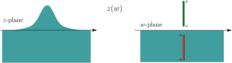
Figure 1: (Schematics of conformal map $z$) The fluid region (green) is mapped to the lower complex plane $\operatorname{Im}w<0$, the branch cut of $R$, $V$ is marked in blue. The branch cuts for complex conjugate functions are marked red.

The nonlinear equations for dynamics of free surface of 2D fluid, written in conformal variables, are known since [Ovsyannikov, 1973, Tanveer, 1991]. We consider the form of these equations given in the work [Dyachenko, 2001]:

$$\dot{R}=i\left(UR^{\prime}-U^{\prime}R\right)$$ (1)

$$\dot{V}=i\left(UV^{\prime}-B^{\prime}R\right)$$ (2)

The functions $R(w,t)$, $V(w,t)$, $U(w,t)$, and $B(w,t)$ are analytic with respect to complex variable $w=u+iv\in\mathbb{C}^{-}$ (the lower half-plane). Here $U(w,t)$ and $B(w,t)$ are analytically continued from the real line, where they are given by the relations:

$$U(u,t)=\hat{P}^{-}[\bar{V}(u,t)R(u,t)+V(u,t)\bar{R}(u,t)],\hskip 20.0ptB(u,t)=\hat{P}^{-}[V(u,t)\bar{V}(u,t)].$$ (3)

Here $\hat{P}^{-}$ is the projection operator from the real axis to the lower half-plane. Given on the real axis

$$\hat{P}^{-}=\frac{1}{2}(1+i\hat{H}),\hskip 10.0pt\hat{H}\hskip 6.0pt\mbox{- is the Hilbert tranform:}\hskip 6.0pt\hat{H}f=p.v.\frac{1}{\pi}\int_{-\infty}^{\infty}\frac{f(u^{\prime},t)du^{\prime}}{u^{\prime}-u}.$$

Let

$$R(w,t)=1+\rho(w,t),\quad\mbox{where}\quad\rho(w\to\infty)\to 0$$ (4)

The four analytic functions have square–root branch points at $w=ia(t)$ and $w=ib(t)$, and thus can be expressed by means of the Cauchy integral formula with the clockwise contour orientation:

$$\rho(w,t)=\frac{1}{2\pi i}\oint\limits_{[ia,ib]}\frac{\rho(s,t)\,ds}{s-w}=\frac{i}{2\pi}\lim\limits_{\varepsilon\to 0^{+}}\int\limits_{ia}^{ib}\frac{\left[\rho(s+\varepsilon)-\rho(s-\varepsilon)\right]ds}{s-w},$$ (5)

and we denote $\rho(s\pm\varepsilon)\to\rho^{\pm}(s)$ as $\varepsilon\to 0^{+}$. Let $\tau=-is\in[a,b]$, then we rewrite the formula as follows:

$$\rho(w,t)=\frac{1}{2\pi}\int\limits_{a}^{b}\frac{\left[\rho^{+}(i\tau)-\rho^{-}(i\tau)\right]d\tau}{-i\tau+w}$$ (6)

and define jumps on the cut for $\rho$ and $V$:

$$r(\tau)=\frac{\rho^{+}(i\tau)-\rho^{-}(i\tau)}{2i}\quad\mbox{and}\quad v(\tau)=\frac{V^{+}(i\tau)-V^{-}(i\tau)}{2i}$$ (7)

and note that $r(a)=r(b)=0$ and $v(a)=v(b)=0$. The associated analytic functions are then given by:

$$R(w,t)=1-\frac{1}{\pi}\int\limits_{a}^{b}\frac{r(\tau)\,d\tau}{\tau+iw}\quad\mbox{and}\quad V(w,t)=-\frac{1}{\pi}\int\limits_{a}^{b}\frac{v(\tau)\,d\tau}{\tau+iw}$$ (8)

We also introduce the two additional functions from the following relations to introduce $U$ and $B$:

$$\bar{R}V+R\bar{V} =V+\bar{V}+\frac{1}{\pi^{2}}\iint\frac{\left[\bar{r}(\tau^{\prime})v(\tau)+r(\tau)\bar{v}(\tau^{\prime})\right]d\tau d\tau^{\prime}}{(\tau+iw)(\tau^{\prime}-iw)},$$ (9)

$$\bar{V}V =\frac{1}{\pi^{2}}\iint\frac{v(\tau)\bar{v}(\tau^{\prime})d\tau d\tau^{\prime}}{(\tau+iw)(\tau^{\prime}-iw)}$$ (10)

We refer the reader to the derivation in Appendix A for derivation of the following formulas:

$$U(w)=-\frac{1}{\pi}\int\frac{u(\tau)d\tau}{\tau+iw}\quad\mbox{and}\quad B(w)=-\frac{1}{\pi}\int\frac{b(\tau)d\tau}{\tau+iw}$$ (11)

where $u(\tau)=v(\tau)\bar{R}(i\tau)+r(\tau)\bar{V}(i\tau)$ and $b(\tau)=v(\tau)\bar{V}(i\tau)$ for $\tau\in[a,b]$.

2.1 Boundary values of analytic function at the cut

Before proceeding, one must be able to evaluate the complex analytic function by its associated jump on the cut. Given $\varepsilon>0$, one finds that

$$R(i\tau\pm\varepsilon)=1-\frac{1}{\pi}\int\limits_{a}^{b}\frac{r(\tau^{\prime})d\tau^{\prime}}{\tau^{\prime}-\tau\pm i\varepsilon}\quad\mbox{and}\quad V(i\tau\pm\varepsilon)=-\frac{1}{\pi}\int\limits_{a}^{b}\frac{v(\tau^{\prime})d\tau^{\prime}}{\tau^{\prime}-\tau\pm i\varepsilon}$$ (12)

and may apply the Sokhotskii–Plemelj theorem to obtain:

$$R^{\pm}(i\tau) =\lim\limits_{\varepsilon\to 0^{+}}R(i\tau\pm\varepsilon)=1-\left(\hat{H}\mp i\right)r(\tau),$$ (13)

$$V^{\pm}(i\tau) =\lim\limits_{\varepsilon\to 0^{+}}V(i\tau\pm\varepsilon)=-\left(\hat{H}\mp i\right)v(\tau),$$ (14)

where we have defined the integral operator $\hat{H}$ as follows:

$$\hat{H}f(\tau)=\frac{1}{\pi}v.p.\int\limits_{a}^{b}\frac{f(\tau^{\prime})d\tau^{\prime}}{\tau^{\prime}-\tau}$$ (15)

Similar relations hold for the functions $U$ and $B$.

2.2 Equations of motion on the cut

The equations of motion in $w$–plane have been derived previously, and are given by:

$$\partial_{t}R =i\left(UR_{w}-U_{w}R\right),$$ (16)

$$\partial_{t}V =i\left(UV_{w}-B_{w}R\right)$$ (17)

and can be written in terms of the jumps of the associated functions as follows:

$$r_{t}+u\hat{H}r^{\prime}+r^{\prime}\hat{H}u+u^{\prime}(1-\hat{H}r)-r\hat{H}u^{\prime} = 0$$ (18)

$$v_{t}+u\hat{H}v^{\prime}+v^{\prime}\hat{H}u+b^{\prime}(1-\hat{H}r)-r\hat{H}b^{\prime} = 0$$ (19)

Given a square-root branch point in $z(w)=\sqrt{w-ia}$, the function $R=1/z_{u}\sim\sqrt{w-ia}$ vanishes at the branch points. Similarly, it is trivial to show that $R(w,t)$ has zeros at the branch points $ia$ and $ib$:

$$R(ia)=R(ib)=0\quad\mbox{and}\quad R(w\to-i\infty)\to 1$$ (20)

as the solution evolves the branch points do not vanish, but move in the complex plane see [Dyachenko et al., 2021].

One can use the shifted Chebyshev basis to efficiently represent the complex analytic functions with a pair of square–root singularities. We introduce the center of the cut, $c(t)=\frac{a(t)+b(t)}{2}$, and its half-length, $l(t)=\frac{b(t)-a(t)}{2}$, and use $f_{n}(w,t)$ as a basis for expansion of the analytic functions $R(w,t)$ and $V(w,t)$. It is convenient to work with the variable $\xi(w,t)=\frac{c+iw}{l}$, then:

$$f_{n}(\xi) =\left[\xi-\sqrt{\xi^{2}-1}\right]^{n}=(-1)^{n}\left[T_{n}(-\xi)+U_{n-1}\left(-\xi\right)\sqrt{\xi^{2}-1}\right],$$ (21)

where $T_{n}(\xi)$ and $U_{n-1}(\xi)$ for $n=1,2,\ldots$ are the Chebyshev polynomials of the first and the second kind respectively. Note that $w\in[ia,ib]$ is mapped to $\xi\in[-1,1]$ for convenience.

2.3 Expansion of $R(w,t)$ and $V(w,t)$

The complex velocity, $V$, and $R$ may be expanded in the form:

$$V(\xi,t)=\sum\limits_{k=1}^{\infty}v_{k}(t)f_{k}(\xi)\quad\mbox{and}\quad R(\xi,t)=1+\sum\limits_{k=1}^{\infty}r_{k}(t)f_{k}(\xi).$$ (22)

In order to satisfy the conditions (20) we have two additional constraints on the coefficients of $R$ that must be satisfied for any $t>0$:

$$\sum\limits_{k=1}^{\infty}r_{k}(t)=\sum\limits_{k=1}^{\infty}(-1)^{k}r_{k}(t)=-1$$

It is convenient to rewrite the series defined in relations (22) and (21) using the following substitution

$$\xi=\cos{\chi}\quad\mbox{or, equivalently}\quad w=ic-il\cos{\chi},\quad\chi=\eta+i\zeta$$ (23)

where $\chi\in[-\pi,\pi]$ is mapped to $\xi\in[-1,1]$. Moreover, the relation (23) defines a conformal mapping for complex $w$, such that $\chi(w\in\mathbb{C})\to\mathbb{C^{-}}$ (see also illustration in Fig 2), and the free surface (blue-white boundary) is located at:

$$\chi(u)=i\ln\left[\xi-\sqrt{\xi^{2}-1}\right],\,\,\,\mbox{where}\,\,\,\xi=\frac{c+iu}{l}.$$ (24)

Note: square root in (24) is so that $\sqrt{a^{2}e^{i\phi}}=|a|e^{i\frac{\phi}{2}}$.

The components of the Chebyshev series:

$$f_{n}(\xi) =\left[\xi-\sqrt{\xi^{2}-1}\right]^{n}=e^{-in\chi},$$ (25)

becomes the standard Fourier series in $\chi$ variable in negative Fourier harmonics. Note that all functions $R$, $V$, $U$, $B$ and their complex conjugates in the $w$-plane can be expanded in the series (25) with $n\geq 0$.

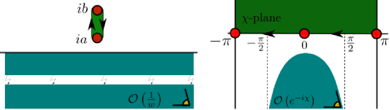
Figure 2: (Schematics of $\chi$-map) A periodic strip $-\pi\leq\operatorname{Re}\chi<\pi$ and $\operatorname{Im}\chi<0$ (right) is mapped to $w\in\mathbb{C}\cap[ia,ib]$ (left), and the $\operatorname{Im}\chi>0$ (right) is mapped to the second sheet of $w$-plane. (Left Panel) The blue region is mapped to the fluid domain (the real fluid), and the upper halfplane marked white excluding the cut is the virtual fluid in the first sheet outside the cut. The red circles mark the location of the branch points, and arrows indicate the positive orientation for a Cauchy-type integral (5). An observer marked with an eye that is located far away from the cut (large distance from real line is illustrated by the lightning symbols) sees the dominant term of a far field $1/w$ whose coefficient is a motion integral defined in (29). The green domain observed on the left is the virtual fluid of the second Riemann sheet which is seen through the cut. (Right Panel) After the conformal map (23) the image of a periodic contour around the cut is mapped to the interval $[-\pi,\pi]$, and the Chebyshev function basis (21) becomes the standard Fourier basis (25). The image of the real fluid is located in the lower complex plane enclosed within vertical asymptotes $\chi=\pm\frac{\pi}{2}$ (dashed lines), and the virtual fluid from the first sheet is mapped to the white region in the lower halfplane. The second Riemann sheet is unfolded into the upper halfplane of the $\chi$-plane. The singularities in the upper half-plane of $\chi$ are located in the second Riemann sheet of $w$-plane, and can be studied numerically and theoretically.

$$V(\chi,t)=\sum\limits_{k=1}^{\infty}v_{k}(t)e^{-ik\chi}\quad\mbox{and}\quad R(\chi,t)=1+\sum\limits_{k=1}^{\infty}r_{k}(t)e^{-ik\chi}.$$ (26)

In order to determine the functions $U$ and $B$ we will first evaluate evaluate the auxiliary functions $u(\tau)$ and $b(\tau)$ at the cut. Then we will use the Sokhotskii-Plemelj Thm to find the values of $U$ and $B$ at the cut, $\chi=\eta+i0\in[-\pi,\pi]$. The values of $R$ and $V$ at the reflection of the contour around the cut in the lower halfplane of $w$ can be determined in the $\chi$-plane. The reflection of the cut is located on the negative imaginary axis at $\chi=0+i\zeta_{cc}(\tau)$ given by the relation:

$$\cos i\zeta_{cc}=\frac{c+\tau}{l},$$

$$\cos i\zeta_{cc}=2+2\frac{a}{l}-\xi=2+2\frac{a}{l}-\cos{\eta}$$

where $\tau\in[a,b]$ (see also the formula (11)). Note that the righthand side of the formula is strictly greater than $1$, and the values of $\zeta_{cc}$ are purely real and negative, given our choice of the mapping $\chi(w)$. Solving for $\zeta_{cc}$, we find:

$$\zeta_{cc}(\xi)=-\ln\left[y+\sqrt{y^{2}-1}\right]=-\operatorname{acosh}{y},$$

where $y=2+2\frac{a}{l}-\xi$. The functions $\bar{R}$ and $\bar{V}$ can then be found on the reflection of the cut $w\in[-ia,-ib]$ (or equivalently $\chi\in i\zeta_{cc}$) by evaluating the formulas:

$$\bar{R}=1-\pi\sum\limits_{k=1}k_{n}\left(\sqrt{y^{2}-1}-y\right)^{k}=1-\pi\sum\limits_{n=1}r_{k}(-1)^{k}e^{k\zeta_{cc}},$$

$$\bar{V}=-\pi\sum\limits_{k=1}v_{k}\left(\sqrt{y^{2}-1}-y\right)^{k}=-\pi\sum\limits_{k=1}v_{k}(-1)^{k}e^{k\zeta_{cc}}.$$

We may now form the functions $u=V\bar{R}+\bar{V}R$ and $b=V\bar{V}$ and find the boundary values of analytic functions $U$ and $B$ as follows:

$$U(\eta)=\frac{1}{2\pi i}\int\limits_{-\pi}^{\pi}\frac{u(-\eta^{\prime})-u(\eta^{\prime})}{2}\cot\frac{\eta^{\prime}-\eta}{2}\,d\eta^{\prime},$$

$$B(\eta)=\frac{1}{2\pi i}\int\limits_{-\pi}^{\pi}\frac{b(-\eta^{\prime})-b(\eta^{\prime})}{2}\cot\frac{\eta^{\prime}-\eta}{2}\,d\eta^{\prime},$$

which can be efficiently computed by means of the fast Fourier transform.

2.4 Equations in $\chi$-plane and integrals of motion

By making additional transformation (23) the equations of motion become particularly simple, and are given by the following relations:

$$-l\sin\eta R_{t}-\left(\dot{c}+\dot{l}\cos\eta\right)R_{\eta}=i\left(UR_{\eta}-U_{\eta}R\right),$$ (27)

$$-l\sin\eta V_{t}-\left(\dot{c}+\dot{l}\cos\eta\right)V_{\eta}=i\left(UV_{\eta}-B_{\eta}R\right).$$ (28)

These equations have two integrals of motion which are equivalent to the ones found in Tanveer [1993]. Indeed, one can integrate equations (27) using expansion (26). As a result, the following expressions are valid:

$$\begin{cases}r_{1}l(t)=-2Q=const\\ v_{1}l(t)\,=-2\Gamma\,=const\end{cases}\Rightarrow\quad e^{-i\chi}=-\frac{l(t)}{2w}\hskip 10.0pt\mbox{as}\hskip 10.0ptw\to\infty$$

or

$$R(w)=1+\frac{Q}{w}+\mathcal{O}\Big{(}\frac{1}{w^{2}}\Big{)},\hskip 20.0ptV(w)=\frac{\Gamma}{w}+\mathcal{O}\Big{(}\frac{1}{w^{2}}\Big{)}\hskip 10.0pt|w|\to\infty$$ (29)

$Q$ and $\Gamma$ are called “winding” and virtual “circulation”. Conservation of circulation can be viewed as Kelvin’s theorem for virtual fluid, and winding is related to the topology of the conformal plane.

2.5 Formation of singularity in infinite time

We shall consider the lowest order expansion so that the initial datum satisfies the constraints (20) and still results in a nontrivial fluid flow. The functions $R$ and $V$ at time $t=0$ are given by:

$$V(\xi) =lf_{1}(\xi)=i\left[w-ic-\sqrt{(w-ic)^{2}+l^{2}}\right]$$ (30)

$$R(\xi) =1-f_{2}(\xi)=\left[1+\frac{1}{l^{2}}\left(w-ic-\sqrt{(w-ic)^{2}+l^{2}}\right)^{2}\right]$$ (31)

It is assumed that at least for some time, these functions are given by convergent series of the form (22), or equivalently the Fourier series (26). This is a crucial assumption that is only based on the results of numerical simulations of the short branch cut [Dyachenko et al., 2021], and preceding theoretical work (see [Tanveer, 1993, Dyachenko et al., 2019]). Vaguely speaking this assumption will hold when the only zeros of $R$ in the first Riemann sheet are located at the branch points. Naturally one must ensure that the initial data (30)-(31) has no additional zeros in the first sheet.

In order to establish the motion of the branch points we seek the complex conjugated functions given by:

$$\tilde{V} =-i\left[w+ic-\sqrt{(w+ic)^{2}+l^{2}}\right],$$ (32)

$$\tilde{R} =\left[1+\frac{1}{l^{2}}\left(w+ic-\sqrt{(w+ic)^{2}+l^{2}}\right)^{2}\right].$$ (33)

Then we must calculate all four functions $V$, $\tilde{V}$, $R$ and $\tilde{R}$ on the imaginary axis by replacing $w\to iv$. We introduce:

$$S =\sqrt{(v-a)(v-b)}=\sqrt{l^{2}-(v-c)^{2}},$$ (34)

$$F =\sqrt{(v+a)(v+b)}=\sqrt{(v+c)^{2}-l^{2}}$$ (35)

Now

$$V =-v+c-iS,$$ (36)

$$\tilde{V} =v+c-F$$ (37)

and we may write

$$R =1-\frac{\left(v-c+iS\right)^{2}}{l^{2}}=\frac{2}{l^{2}}\left[S^{2}-i(v-c)S\right],$$ (38)

$$\tilde{R} =1-\frac{\left(v+c-F\right)^{2}}{l^{2}}=\frac{2}{l^{2}}F\left(v+c-F\right)$$ (39)

Then we introduce

$$Q=R\tilde{V}+\tilde{R}V$$ (40)

to end up with transport velocity $U$:

$$U=P^{-}Q$$ (41)

Notice that the singularities of $Q$ in the upper half–plane are the ones coming from the function $S$. We can replace $Q\to Q_{ess}$ where $Q_{ess}$ only includes the terms proportional to $S$. A simple calculation reveals the following expression:

$$Q_{ess}=\frac{2i}{l^{2}}\left[2lFS-\left(c^{2}+ab+2cv\right)S\right]$$ (42)

Then

$$U=\left(1-i\hat{H}\right)Q_{ess},$$ (43)

where $\hat{H}$ is the Hilbert transform. To calculate the “Hilbert” transform one should remember that after projecting to the lower half–plane $Q_{ess}$ must be replaced by its analytic continuation to the upper half–plane. This is done by restoring the regular part by the corresponding singular part as in formula (21). It amounts to writing:

$$iS \to iS-(v-c),$$ (44)

$$ivS \to ivS-v(v-c)+\frac{1}{2}l^{2}$$ (45)

Collecting all terms together we find following expression for transport velocity $U$:

$$U=Q_{ess}+\frac{2}{l^{2}}\left[2cv^{2}+abv-c\left(c^{2}+\frac{l^{2}}{2}+ab\right)+2cI\right]$$ (46)

where

$$I(v)=\frac{1}{\pi}v.p.\int\limits_{a}^{b}\frac{\sqrt{(s^{2}-a^{2})(b^{2}-s^{2})}\,ds}{s-v}$$ (47)

Now we calculate $U(a)$. As long as $S(a)=0$ this expression is purely real. After tedious calculations we find that

$$U(\varepsilon)=\frac{8b}{(1-\varepsilon)^{2}}\left[-\frac{1}{4}-\varepsilon+\frac{1}{2}\varepsilon^{2}+\varepsilon^{3}+I(\varepsilon)\right],$$ (48)

here $\varepsilon=\frac{a}{b}$ and

$$I(\varepsilon)=\frac{1}{\pi}\int\limits_{\varepsilon}^{1}\sqrt{\frac{(q+\varepsilon)(1-q^{2})}{q-\varepsilon}}\,dq$$ (49)

This integral is expressed in terms of elliptic functions, but we will not provide explicit formulas. We study asymptotic behaviour of $I(\varepsilon)$ at $\varepsilon\to 0$. To do this we use the expansion:

$$\sqrt{\frac{q+\varepsilon}{q-\varepsilon}}=1+\frac{\varepsilon}{q}+\sum\limits_{k=0}^{\infty}c_{k}\left(\frac{\varepsilon}{q}\right)^{k+2}$$ (50)

Thus we must estimate the integral:

$$I(\varepsilon)=\frac{1}{\pi}\int\limits_{\varepsilon}^{1}\left(1+\frac{\varepsilon}{q}+\sum\limits_{k=0}^{\infty}c_{k}\left(\frac{\varepsilon}{q}\right)^{k+2}\right)\sqrt{1-q^{2}}\,dq.$$ (51)

Now we mention that

$$\frac{1}{\pi}\int\limits_{0}^{1}\sqrt{1-q^{2}}\,dq=\frac{1}{4}$$ (52)

One can show that

$$U(\varepsilon)=8b\left(-\frac{1}{4}+\frac{1}{4}+\frac{1}{\pi}\varepsilon\ln\varepsilon+O(\varepsilon)\right),$$ (53)

and therefore:

$$U(\varepsilon)=\frac{8b}{\pi}\varepsilon\ln\varepsilon+O(\varepsilon),$$ (54)

where $O(\varepsilon)$ denote terms of order $\varepsilon$ and all higher orders. It is not necessary to determine them precisely.

We ended up with the following result:

$$U(a)\to\frac{8}{\pi}a\ln\frac{a}{b}+O(a)\,\mbox{at}\,a\to 0.$$ (55)

The differential equation:

$$\dot{a}=\frac{8}{\pi}a\ln\frac{a}{b}$$ (56)

with initial data:

$$\ln\frac{a}{b}=-\ln\frac{b}{a_{0}}=-c$$ (57)

gives solution

$$\ln\frac{a}{b}=-ce^{\frac{8t}{\pi}},$$ (58)

and

$$a=be^{-ce^{\frac{8t}{\pi}}}\,\quad c=-\ln\frac{b}{a_{0}}$$ (59)

It means that singularity $a=0$ is never achieved in a finite time, while it is approaching to the real line faster than exponential estimates predict.

It is important to emphasize that this conclusion will hold only provided that no singularity from the second sheet crosses the branch cut and invalidates the assumptions of single pair of branch points in the first Riemann sheet. Nevertheless, numerical evidence suggests that at least one such solution does exist, see the Fig. $2a$ in [Dyachenko et al., 2021]

3 Conclusion

A potential fluid flow in 2D Euler equations with a free boundary is considered with $V$ and $R$ having a pair of square–root branch points $w=ia$ and $w=ib$ in conformal plane. We obtained the following main results:

• The equations of motion have been transplanted to the cut connecting $ia$ to $ib$ in $w$–plane, and introduced a new conformal mapping $\chi(w)$ that allows the study of singularities in higher Riemann sheets. With the second sheet of $w$-plane unfolded, one can study the singularities in multiple sheets, and possibly obtain new integrals of motion from pairs of cuts in higher sheets. This conjecture will have implications for a further study of integrability of water waves.

• We developed an asymptotic theory based on the exact equations formulated at the cut that shows double–exponential rate of approach of singularity at $w=ia(t)$ to the fluid domain. The presented theory answers a long–standing question about formation of singularity at the free surface in finite vs. infinite time when no gravity or capillarity is present. However, it remains unclear whether a solution with only a single pair of branch points in the first sheet can exist for infinite time.

• The physical fluid can be complemented with a virtual fluid, which is a mathematical object whose motion is defined by the analytic continuation of $R$ and $V$ into $\mathbb{C}^{+}$ excluding the branch cut. The expanded domain contains a virtual fluid vortex sheet, for which Kelvin’s theorem for circulation holds true: a “virtual circulation” is conserved and is one of the two new invariants discovered in this work. The second invariant, the “winding”, is related to the genus of conformal plane of the virtual fluid – the number of holes.

The present work offers a new look at the problem of water waves and illustrates a deeply rooted connection between water waves and vortex sheet problem that was overlooked by the water waves community. Despite the fact that the present work is devoted to only a pair of square–root branch points, one may consider a general system of many pairs of branch points connected by branch cuts, $\gamma_{k}(t)$. The equations for analytic functions $R$ and $V$ are then formed at each $\gamma_{k}(t)$ and fully determine the flow of “virtual fluid”. Each of the branch cuts, $\gamma_{k}(t)$ is equivalent to a “virtual” vortex sheet, whose dynamics is governed by 2D Euler equations. An open question one could address is related to the rolling of a vortex sheet: Is breaking of a steep water wave related to instabilities of a “virtual” vortex sheet? The answer to this question is presently a work in progress.

Each pair of square–root branch points is associated with a new pair of integrals of motion: “winding” and virtual “circulation”. A particle analogy springs into mind. Nevertheless these invariants alone do not fully describe the fluid flow, this follows from equations (27), which requires all Fourier modes to be defined, however “winding” and ”circulation” only define the first Fourier modes of $R$ and $V$. Nevertheless, the conformal domain $\chi(w)$ opens the second Riemann sheet for $R$ and $V$ which must contain more singularities and fully define the analytic functions $R$ and $V$ at the cuts. We conjecture that tracking of all singularities and their associated invariants uniquely describes the fluid flow, and are analogous to the “action” variables in the long standing problem of integrability of 2D potential Euler equations.

4 Acknowledgements

Studies presented in it he subsections 2.4 and 2.5 were supported by the Russian Science Foundation grant no. 19-72-30028. The work of V. E. Zakharov was supported by the National Science Foundation, grant no. DMS-1715323. The work of S. A. Dyachenko was supported by the National Science Foundation, grants no. DMS-1716822 and no. DMS-2039071. This material is based upon the work supported by the National Science Foundation under Grant No. DMS-1439786 while S. A. Dyachenko was in residence at the Institute for Computational and Experimental Research in Mathematics in Providence, RI, during a part of the Hamiltonian Methods in Dispersive and Wave Evolution Equations program.

Declaration of Interests. The authors report no conflict of interest.

Appendix A Derivation of $U$ and $B$

We will provide a derivation for the function $B$, and a calculation for $U$ can be done analogously. Let us consider the product:

$$\bar{V}V=\frac{1}{\pi^{2}}\iint\frac{v(\tau)\bar{v}(\tau^{\prime})d\tau d\tau^{\prime}}{(\tau+iw)(\tau^{\prime}-iw)}$$ (60)

and use the relation:

$$\frac{1}{(\tau+iw)(\tau^{\prime}-iw)}=\frac{1}{\tau+\tau^{\prime}}\left[\frac{1}{\tau+iw}+\frac{1}{\tau^{\prime}-iw}\right].$$ (61)

The product $\bar{V}V$ then becomes:

$$\bar{V}V=\frac{1}{\pi}\int\left[\frac{1}{\pi}\int\frac{\bar{v}(\tau^{\prime})d\tau^{\prime}}{\tau^{\prime}+\tau}\right]\frac{v(\tau)d\tau}{\tau+iw}+\frac{1}{\pi}\int\left[\frac{1}{\pi}\int\frac{v(\tau)d\tau}{\tau+\tau^{\prime}}\right]\frac{\bar{v}(\tau)d\tau^{\prime}}{\tau^{\prime}-iw}$$ (62)

One can observe that the terms enclosed in square bracket are given by the following:

$$V(-i\tau^{\prime})=-\frac{1}{\pi}\int\frac{v(\tau)d\tau}{\tau+\tau^{\prime}}\quad\mbox{and}\quad\bar{V}(i\tau)=-\frac{1}{\pi}\int\frac{\bar{v}(\tau^{\prime})d\tau^{\prime}}{\tau^{\prime}+\tau}$$ (63)

and result in the following formula for $\bar{V}V$:

$$\bar{V}V=-\frac{1}{\pi}\int\frac{v(\tau)\bar{V}(i\tau)d\tau}{\tau+iw}-\frac{1}{\pi}\int\frac{\bar{v}(\tau)V(-i\tau)}{\tau-iw}=\hat{P}^{-}\left[\bar{V}V\right]+\hat{P}^{+}\left[\bar{V}V\right],$$ (64)

Thus the function $B(w)$ is defined in the complex plane via:

$$B(w)=-\frac{1}{\pi}\int\frac{v(\tau)\bar{V}(i\tau)d\tau}{\tau+iw}=-\frac{1}{\pi}\int\frac{b(\tau)d\tau}{\tau+iw}$$ (65)

where we defined $b(\tau):=v(\tau)\bar{V}(i\tau)$ at the interval $\tau\in[a,b]$ to be the jump at the branch cut. Analogous calculation for $U$ results in:

$$U(w)=-\frac{1}{\pi}\int\frac{u(\tau)d\tau}{\tau+iw}=-\frac{1}{\pi}\int\frac{\left[v(\tau)\bar{R}(i\tau)+r(\tau)\bar{V}(i\tau)\right]d\tau}{\tau+iw},$$ (66)

where we defined $u(\tau):=v(\tau)\bar{R}(i\tau)+r(\tau)\bar{V}(i\tau)$ at the interval $\tau\in[a,b]$.

Appendix B Supplemental Relations with Chebyshev Polynomials

We consider an auxiliary contour integral around interval $[-1,1]$ and apply residue theorem:

$$I=\oint\limits_{[-1,1]}\frac{\left(T_{n}(x)+\sqrt{x^{2}-1}\,U_{n-1}(x)\right)\,dx}{x+y}=\oint\limits_{[-1,1]}\frac{\left(x+\sqrt{x^{2}-1}\,\right)^{n}\,dx}{x+y},$$ (67)

where we used the following identity for Chebyshev polynomials:

$$T_{n}(x)+\sqrt{x^{2}-1}\,U_{n-1}(x)=\left(x+\sqrt{x^{2}-1}\right)^{n}.$$ (68)

We consider branch of square–root $\sqrt{x^{2}-1}=i\sqrt{1-x^{2}}$ above the cut, and $\sqrt{x^{2}-1}=-i\sqrt{1-x^{2}}$ below. The axiliary integral $I$ is related to integral of interest by the following formula:

$$\int\limits_{-1}^{1}\frac{\sqrt{1-x^{2}}\,U_{n-1}(x)\,dx}{x+y}=\frac{1}{2i}\oint\limits_{[-1,1]}\frac{\left(T_{n}(x)+\sqrt{x^{2}-1}\,U_{n-1}(x)\right)\,dx}{\xi+y}=\frac{I}{2i},$$ (69)

where we have noted that integral of regular function $\frac{T_{n}(x)}{x+y}$ around a closed curve vanishes. The contour integral $I$ consists of four parts, however circular integrals around $x=\pm 1$ vanish because the integrand has no poles at these points, therefore leaving only the two integrals above and below cut:

$$I=\int\limits_{-1}^{1}\frac{\left(x+i\sqrt{1-x^{2}}\right)^{n}-\left(x-i\sqrt{1-x^{2}}\right)^{n}}{x+y}\,dx.$$ (70)

We make a substitution $x=\cos t$, $0<t<\pi$ and symmetrize the interval of integration:

$$I=\int\limits_{\pi}^{0}\frac{e^{int}-e^{-int}}{\cos(t)+y}(-\sin t)\,dt=\frac{1}{2}\int\limits_{-\pi}^{\pi}\frac{e^{int}-e^{-int}}{\cos t+y}\sin t\,dt,$$ (71)

and after the substitution $z=e^{it}$, $|z|=1$ and $dt=\frac{dz}{iz}$:

$$I=-\frac{1}{2}\oint\limits_{|z|=1}\frac{\left(z^{n}-z^{-n}\right)\left(z-z^{-1}\right)}{z^{2}+2yz+1}\,dz.$$ (72)

The integrand has pole of order $(n+3)$ at $z=0$ and a pair of simple poles at $z=-y\pm\sqrt{y^{2}-1}$. When $y=\xi+2+\frac{2a}{l}>1$ and only the poles at $z=0$ and $z=-y+\sqrt{y^{2}-1}$ lie within the unit circle. Note that if $y<-1$ the poles switch.

Note that poles switch if $y<-1$! Also it is straightforward to obtain result for complex $y$.

The residues at $z=-y\pm\sqrt{y^{2}-1}$ can be computed explicitly and by virtue of (68) are given by:

$$\operatorname*{Res}_{-y\pm\sqrt{y^{2}-1}}\frac{(z^{n}-z^{-n})(z-z^{-1})}{z^{2}+2yz+1}=\pm 2\sqrt{y^{2}-1}\,U_{n-1}(-y),$$ (73)

where we used symmetry for Chebyshev polynomials of even and odd $n$.

For the residue at zero we first note the generating function of Chebyshev polynomials:

$$\frac{(z^{n}-z^{-n})(z-z^{-1})}{1+2yz+z^{2}}=\left(z^{n}-\frac{1}{z^{n}}\right)\left(z-\frac{1}{z}\right)\sum\limits_{k=0}^{\infty}U_{k}(-y)z^{k},$$ (74)

to write Laurent series, and note that only the following terms contribute to the principal part:

$$\frac{1}{z^{n+1}}\sum\limits_{k=0}^{\infty}U_{k}(-y)z^{k}-\frac{1}{z^{n-1}}\sum\limits_{k=0}^{\infty}U_{k}(-y)z^{k},$$ (75)

and the residues are:

$$\begin{cases}U_{1}(-y),&n=1\\ U_{n}(-y)-U_{n-2}(-y),&n>1.\end{cases}$$ (76)

It is convenient to use recursion relations for Chebyshev polynomials $2T_{n}(x)=U_{n}(x)-U_{n-2}(x)$ and $2T_{1}(x)=U_{1}(x)$ to have the residue written in the compact form:

$$\operatorname*{Res}_{z=0}\frac{(z^{n}-z^{-n})(z-z^{-1})}{z^{2}+2yz+1}=2T_{n}(-y).$$ (77)

The final result for $y>1$ is obtained by summing the two residues (73) and (77):

$$\frac{1}{\pi}\int\limits_{-1}^{1}\frac{\sqrt{1-x^{2}}\,U_{n-1}(x)\,dx}{x+y}=-\left[T_{n}(-y)+\sqrt{y^{2}-1}\,U_{n-1}(-y)\right]=-\left(\sqrt{y^{2}-1}-y\right)^{n},$$ (78)

Note that this can be extended for $-1<y<1$, and as follows:

$$\frac{1}{\pi}p.v.\int\limits_{-1}^{1}\frac{\sqrt{1-x^{2}}\,U_{n-1}(x)\,dx}{x-y}=-T_{n}(y).$$ (79)

References

- Kolmogorov [1954] A. N. Kolmogorov. On the conservation of conditionally periodic motions under small perturbation of the hamiltonian. 98(527):2–3, 1954.
- Gardner et al. [1967] C. S. Gardner, J. M. Greene, M. D. Kruskal, and R. M. Miura. Method for solving the korteweg-devries equation. Physical review letters, 19(19):1095, 1967.
- Zakharov and Faddeev [1971] Vladimir Evgen’evich Zakharov and Lyudvig Dmitrievich Faddeev. Korteweg–de vries equation: A completely integrable hamiltonian system. Funktsional’nyi Analiz i ego Prilozheniya, 5(4):18–27, 1971.
- Shabat and Zakharov [1972] Aleksei Shabat and Vladimir Zakharov. Exact theory of two-dimensional self-focusing and one-dimensional self-modulation of waves in nonlinear media. Sov. Phys. JETP, 34(1):62, 1972.
- Zakharov and Shabat [1974] Vladimir Evgen’evich Zakharov and Alexey Borisovich Shabat. A scheme for integrating the nonlinear equations of mathematical physics by the method of the inverse scattering problem. i. Funktsional’nyi Analiz i ego Prilozheniya, 8(3):43–53, 1974.
- Ablowitz et al. [1974] M. J. Ablowitz, D. J. Kaup, A. C. Newell, and H. Segur. The inverse scattering transform-fourier analysis for nonlinear problems. Studies in Applied Mathematics, 53(4):249–315, 1974.
- Zakharov and Shabat [1979] V. E. Zakharov and A. B. Shabat. Integration of nonlinear equations of mathematical physics by the method of inverse scattering. ii. Functional Analysis and Its Applications, 13(3):166–174, 1979.
- Dyachenko et al. [1995] A. I. Dyachenko, Y. V. Lvov, and V. E. Zakharov. Five-wave interaction on the surface of deep fluid. Physica D: Nonlinear Phenomena, 87(1-4):233–261, 1995.
- Tanveer [1993] S. Tanveer. Singularities in the classical rayleigh-taylor flow: formation and subsequent motion. Proceedings of the Royal Society of London A: Mathematical, Physical and Engineering Sciences, 441(1913):501–525, 1993.
- Dyachenko et al. [2019] A. I. Dyachenko, S. A. Dyachenko, P. M. Lushnikov, and V. E. Zakharov. Dynamics of poles in two-dimensional hydrodynamics with free surface: new constants of motion. Journal of Fluid Mechanics, 874:891–925, 2019. 10.1017/jfm.2019.448.
- Lushnikov and Zakharov [2021] P. M. Lushnikov and V. E. Zakharov. Poles and branch cuts in free surface hydrodynamics. Water Waves, 3:251–266, 2021.
- Dyachenko et al. [2021] AI Dyachenko, SA Dyachenko, PM Lushnikov, and VE Zakharov. Short branch cut approximation in two-dimensional hydrodynamics with free surface. Proceedings of the Royal Society A, 477(2249):20200811, 2021.
- Polubarinova-Kochina [1945] P. Ya. Polubarinova-Kochina. On the displacement of the oil-bearing contour. Comptes Rendus (Doklady) de L’Academie des Sciences de l’URSS, 47:250–254, 1945.
- Galin [1945] L. A. Galin. Unsteady filtration with a free surface. Comptes Rendus (Doklady) de L’Academie des Sciences de l’URSS, 47:246––249, 1945.
- Zakharov and Dyachenko [1996] V. E. Zakharov and A. I. Dyachenko. High-jacobian approximation in the free surface dynamics of an ideal fluid. Physica D: Nonlinear Phenomena, 98(2):652–664, 1996.
- Longuet-Higgins [1972] M. S. Longuet-Higgins. A class of exact, time-dependent, free-surface flows. Journal of Fluid Mechanics, 55(3):529–543, 1972.
- Crapper [1957] G. D. Crapper. An exact solution for progressive capillary waves of arbitrary amplitude. Journal of Fluid Mechanics, 2:532–540, 1957. 10.1017/S0022112057000348.
- Crowdy [2000] Darren G Crowdy. A new approach to free surface euler flows with capillarity. Studies in Applied Mathematics, 105(1):35–58, 2000.
- Dyachenko and Mikyoung Hur [2019] S. A. Dyachenko and V. Mikyoung Hur. Stokes waves with constant vorticity: folds, gaps and fluid bubbles. Journal of Fluid Mechanics, 878:502–521, 2019.
- Mikyoung Hur and Wheeler [2020] V. Mikyoung Hur and M. H. Wheeler. Exact free surfaces in constant vorticity flows. Journal of Fluid Mechanics, 896, 2020.
- Baker and Xie [2011] G. R. Baker and C. Xie. Singularities in the complex physical plane for deep water waves. Journal of Fluid Mechanics, 685:83–116, 2011. 10.1017/jfm.2011.283.
- Dyachenko and Newell [2016] S. A. Dyachenko and A. C. Newell. Whitecapping. Studies in Applied Mathematics, 137(2):199–213, 2016.
- Castro et al. [2013] Angel Castro, Diego Córboda, Charles Fefferman, Francisco Gancedo, and Javier Gómez-Serrano. Finite time singularities for the free boundary incompressible euler equations. Annals of Mathematics, pages 1061–1134, 2013.
- Kuznetsov et al. [1993] E. A. Kuznetsov, M. D. Spector, and V. E. Zakharov. Surface singularities of ideal fluid. Physics Letters A, 182(4-6):387–393, 1993.
- Karabut and Zhuravleva [2014] E. A. Karabut and E. N. Zhuravleva. Unsteady flows with a zero acceleration on the free boundary. Journal of Fluid Mechanics, 754:308–331, 2014. 10.1017/jfm.2014.401.
- Karabut et al. [2020] E. A. Karabut, E. N. Zhuravleva, and N. M. Zubarev. Application of transport equations for constructing exact solutions for the problem of motion of a fluid with a free boundary. Journal of Fluid Mechanics, 890, 2020.
- Dyachenko et al. [1996a] A. I. Dyachenko, V. E. Zakharov, and E. A. Kuznetsov. Nonlinear dynamics of the free surface of an ideal fluid. Plasma Physics Reports, 22(10):829–840, 1996a.
- Dyachenko et al. [1996b] A. I. Dyachenko, E. A. Kuznetsov, M. D. Spector, and V. E. Zakharov. Analytical description of the free surface dynamics of an ideal fluid (canonical formalism and conformal mapping). Physics Letters A, 221(1):73 – 79, 1996b.
- Zakharov [2020] V. E. Zakharov. Integration of a deep fluid equation with a free surface. Theoretical & Mathematical Physics, 202(3), 2020.
- Liu and Pego [2021] Jian-Guo Liu and R. L. Pego. In search of local singularities in ideal potential flows with free surface. arXiv preprint arXiv:2108.00445, 2021.
- Grant [1973] M. A. Grant. The singularity at the crest of a finite amplitude progressive stokes wave. Journal of Fluid Mechanics, 59(2):257–262, 1973.
- Dyachenko et al. [2014] S. A. Dyachenko, P. M. Lushnikov, and A. O. Korotkevich. Complex singularity of a stokes wave. JETP letters, 98(11):675–679, 2014.
- Dyachenko et al. [2016] S. A. Dyachenko, P. M. Lushnikov, and A. O. Korotkevich. Branch cuts of stokes wave on deep water. part i: numerical solution and padé approximation. Studies in Applied Mathematics, 137(4):419–472, 2016.
- Alpert et al. [2000] B. Alpert, L. Greengard, and T. Hagström. Rapid evaluation of nonreflecting boundary kernels for time-domain wave propagation. SIAM Journal on Numerical Analysis, 37(4):1138–1164, 2000.
- Lushnikov [2016] P. M. Lushnikov. Structure and location of branch point singularities for stokes waves on deep water. Journal of Fluid Mechanics, 800:557–594, 2016.
- Stokes [1880] G. G. Stokes. Mathematical and Physical Papers, volume 1. Cambridge University Press, 1880.
- Haziot et al. [2021] S. V. Haziot, V. Mikyoung Hur, W. Strauss, J. F. Toland, E. Wahlén, S. Walsh, and M. H. Wheeler. Traveling water waves – the ebb and flow of two centuries. 2021.
- Wilkening [2021] J. Wilkening. Traveling-standing water waves. Fluids, 6(5), 2021. ISSN 2311-5521. 10.3390/fluids6050187.
- Ovsyannikov [1973] L. V. Ovsyannikov. Dynamika sploshnoi sredy, lavrentiev institute of hydrodynamics. Sib. Branch Acad. Sci. USSR, 15:104, 1973.
- Zakharov [1968] V. E. Zakharov. Stability of periodic waves of finite amplitude on the surface of a deep fluid. Journal of Applied Mechanics and Technical Physics, 9(2):190–194, Mar 1968.
- Wilkening and Vasan [2015] J. Wilkening and V. Vasan. Comparison of five methods of computing the dirichlet-neumann operator for the water wave problem. Contemp. Math, 635:175–210, 2015.
- Arsénio et al. [2020] D. Arsénio, E. Dormy, and C. Lacave. The vortex method for two-dimensional ideal flows in exterior domains. SIAM Journal on Mathematical Analysis, 52(4):3881–3961, 2020.
- Ambrose et al. [2021] David M. Ambrose, Roberto Camassa, Jeremy L. Marzuola, Richard M. McLaughlin, Quentin Robinson, and Jon Wilkening. Numerical algorithms for water waves with background flow over obstacles and topography, 2021.
- Tanveer [1991] S. Tanveer. Singularities in water waves and rayleigh–taylor instability. Proceedings of the Royal Society of London. Series A: Mathematical and Physical Sciences, 435(1893):137–158, 1991.
- Dyachenko [2001] A. I. Dyachenko. On the dynamics of an ideal fluid with a free surface. Dokl. Math., 63:115–117, 2001.
- Zakharov et al. [2002] V. E. Zakharov, A. I. Dyachenko, and O. A. Vasilyev. New method for numerical simulation of a nonstationary potential flow of incompressible fluid with a free surface. European Journal of Mechanics - B/Fluids, 21(3):283 – 291, 2002.