Differentially Private Aggregation in the Shuffle Model:
Almost Central Accuracy in Almost a Single Message

Abstract

The shuffle model of differential privacy has attracted attention in the literature due to it being a middle ground between the well-studied central and local models. In this work, we study the problem of summing (aggregating) real numbers or integers, a basic primitive in numerous machine learning tasks, in the shuffle model. We give a protocol achieving error arbitrarily close to that of the (Discrete) Laplace mechanism in the central model, while each user only sends $1+o(1)$ short messages in expectation.

1 Introduction

A principal goal within trustworthy machine learning is the design of privacy-preserving algorithms. In recent years, differential privacy (DP) Dwork et al. (2006b; a) has gained significant popularity as a privacy notion due to the strong protections that it ensures. This has led to several practical deployments including by Google Erlingsson et al. (2014); Shankland (2014), Apple Greenberg (2016); Apple Differential Privacy Team (2017), Microsoft Ding et al. (2017), and the U.S. Census Bureau Abowd (2018). DP properties are often expressed in terms of parameters $\varepsilon$ and $\delta$, with small values indicating that the algorithm is less likely to leak information about any individual within a set of $n$ people providing data. It is common to set $\varepsilon$ to a small positive constant (e.g., $1$), and $\delta$ to inverse-polynomial in $n$.

DP can be enforced for any statistical or machine learning task, and it is particularly well-studied for the real summation problem, where each user $i$ holds a real number $x_{i}\in[0,1]$, and the goal is to estimate $\sum_{i}x_{i}$. This constitutes a basic building block within machine learning, with extensions including (private) distributed mean estimation (see, e.g., Biswas et al., 2020; Girgis et al., 2021), stochastic gradient descent  Song et al. (2013); Bassily et al. (2014); Abadi et al. (2016); Agarwal et al. (2018), and clustering Stemmer & Kaplan (2018); Stemmer (2020).

The real summation problem, which is the focus of this work, has been well-studied in several models of DP. In the central model where a curator has access to the raw data and is required to produce a private data release, the smallest possible absolute error is known to be $O(1/\varepsilon)$; this can be achieved via the ubiquitous Laplace mechanism Dwork et al. (2006b), which is also known to be nearly optimal for the most interesting regime of $\varepsilon\leq 1$. In contrast, for the more privacy-stringent local setting Kasiviswanathan et al. (2008) (also Warner, 1965) where each message sent by a user is supposed to be private, the smallest error is known to be $\Theta_{\varepsilon}(\sqrt{n})$ Beimel et al. (2008); Chan et al. (2012). This significant gap between the achievable central and local utilities has motivated the study of intermediate models of DP. The shuffle model Bittau et al. (2017); Erlingsson et al. (2019); Cheu et al. (2019) reflects the setting where the user reports are randomly permuted before being passed to the analyzer; the output of the shuffler is required to be private. Two variants of the shuffle model have been studied: in the multi-message case (e.g., Cheu et al., 2019), each user can send multiple messages to the shuffler; in the single-message setting each user sends one message (e.g., Erlingsson et al., 2019; Balle et al., 2019).

For the real summation problem, it is known that the smallest possible absolute error in the single-message shuffle model is $\tilde{\Theta}_{\varepsilon}(n^{1/6})$ Balle et al. (2019). In contrast, multi-message shuffle protocols exist with a near-central accuracy of $O(1/\varepsilon)$ Ghazi et al. (2020c); Balle et al. (2020), but they suffer several drawbacks in that the number of messages sent per user is required to be at least $3$, each message has to be substantially longer than in the non-private case, and in particular, the number of bits of communication per user has to grow with $\log(1/\delta)/\log n$. This (at least) three-fold communication blow-up relative to a non-private setting can be a limitation in real-time reporting use cases (where encryption of each message may be required and the associated cost can become dominant) and in federated learning settings (where great effort is undertaken to compress the gradients). Our work shows that near-central accuracy and near-zero communication overhead are possible for real aggregation over sufficiently many users:

Theorem 1.

For any $0<\varepsilon\leq O(1),\zeta,\delta\in(0,1/2)$, there is an $(\varepsilon,\delta)$-DP real summation protocol in the shuffle model whose mean squared error (MSE) is at most the MSE of the Laplace mechanism with parameter $(1-\zeta)\varepsilon$, each user sends $1+\tilde{O}_{\zeta,\varepsilon}\left(\frac{\log(1/\delta)}{\sqrt{n}}\right)$ messages in expectation, and each message contains $\tfrac{1}{2}\log n+O(\log\frac{1}{\zeta})$ bits.

Note that $\tilde{O}_{\zeta,\varepsilon}$ hides a small $\mathrm{poly}(\log n,1/\varepsilon,1/\zeta)$ term. Moreover, the number of bits per message is equal, up to lower order terms, to that needed to achieve MSE $O(1)$ even without any privacy constraints.

Theorem 1 follows from an analogous result for the case of integer aggregation, where each user is given an element in the set $\{0,1,...,\Delta\}$ (with $\Delta$ an integer), and the goal of the analyzer is to estimate the sum of the users’ inputs. We refer to this task as the $\Delta$-summation problem.

For $\Delta$-summation, the standard mechanism in the central model is the Discrete Laplace (aka Geometric) mechanism, which first computes the true answer and then adds to it a noise term sampled from the Discrete Laplace distribution with parameter $\varepsilon/\Delta$ Ghosh et al. (2012). We can achieve an error arbitrarily close to this mechanism in the shuffle model, with minimal communication overhead:

Theorem 2.

For any $0<\varepsilon\leq O(1),\gamma,\delta\in(0,1/2),\Delta\in\mathbb{N}$, there is an $(\varepsilon,\delta)$-DP $\Delta$-summation protocol in the shuffle model whose MSE is at most that of the Discrete Laplace mechanism with parameter $(1-\gamma)\varepsilon/\Delta$, and where each user sends $1+\tilde{O}\left(\frac{\Delta\log(1/\delta)}{\gamma\varepsilon n}\right)$ messages in expectation, with each message containing $\lceil\log\Delta\rceil+1$ bits.

In Theorem 2, the $\tilde{O}(\cdot)$ hides a $\mathrm{poly}\log\Delta$ factor. We also note that the number of bits per message in the protocol is within a single bit from the minimum message length needed to compute the sum without any privacy constraints. Incidentally, for $\Delta=1$, Theorem 2 improves the communication overhead obtained by Ghazi et al. (2020b) from $O\left(\frac{\log^{2}(1/\delta)}{\varepsilon^{2}n}\right)$ to $O\left(\frac{\log(1/\delta)}{\varepsilon n}\right)$. (This improvement turns out to be crucial in practice, as our experiments show.)

Using Theorem 1 as a black-box, we obtain the following corollary for the $1$-sparse vector summation problem, where each user is given a $1$-sparse (possibly high-dimensional) vector of norm at most $1$, and the goal is to compute the sum of all user vectors with minimal $\ell_{2}$ error.

Corollary 3.

For every $d\in\mathbb{N}$, and $0<\varepsilon\leq O(1),\zeta,\delta\in(0,1/2)$, there is an $(\varepsilon,\delta)$-DP algorithm for $1$-sparse vector summation in $d$ dimensions in the shuffle model whose $\ell_{2}$ error is at most that of the Laplace mechanism with parameter $(1-\zeta)\varepsilon/2$, and where each user sends $1+\tilde{O}_{\zeta,\varepsilon}\left(\frac{d\log(1/\delta)}{\sqrt{n}}\right)$ messages in expectation, and each message contains $\log{d}+\tfrac{1}{2}\log n+O(\log\frac{1}{\zeta})$ bits.

1.1 Technical Overview

We will now describe the high-level technical ideas underlying our protocol and its analysis. Since the real summation protocol can be obtained from the $\Delta$-summation protocol using known randomized discretization techniques (e.g., from Balle et al. (2020)), we focus only on the latter. For simplicity of presentation, we will sometimes be informal here; everything will be formalized later.

Infinite Divisibility.

To achieve a similar performance to the central-DP Discrete Laplace mechanism (described before Theorem 2) in the shuffle model, we face several obstacles. To begin with, the noise has to be divided among all users, instead of being added centrally. Fortunately, this can be solved through the infinite divisibility of Discrete Laplace distributions: there is a distribution $\mathcal{D}^{\prime}$ for which, if each user $i$ samples a noise $z_{i}$ independently from $\mathcal{D}^{\prime}$, then $z_{1}+\cdots+z_{n}$ has the same distribution as $\operatorname{DLap}(\varepsilon/\Delta)$.

To implement the above idea in the shuffle model, each user has to be able to send their noise $z_{i}$ to the shuffler. Following Ghazi et al. (2020b), we can send such a noise in unary, i.e., if $z_{i}>0$ we send the $+1$ message $z_{i}$ times and otherwise we send the $-1$ message $-z_{i}$ times. This is in addition to user $i$ sending their own input $x_{i}$ (in binary, as a single message) if it is non-zero. The analyzer is simple: sum up all the messages.

Unfortunately, this zero-sum noise approach is not shuffle DP for $\Delta>1$ because, even after shuffling, the analyzer can still see $u_{j}$, the number of messages $j$, which is exactly the number of users whose input is equal to $j$ for $j\in\{2,\dots,\Delta\}$.

Zero-Sum Noise over Non-Binary Alphabets.

To overcome this issue, we have to ‘noise” the values $u_{j}$ themselves, while at the same time preserving the accuracy. We achieve this by making some users send additional messages whose sum is equal to zero; e.g., a user may send $-1,-1,+2$ in conjunction with previously described messages. Since the analyzer just sums up all the messages, this additional zero-sum noise still does not affect accuracy.

The bulk of our technical work is in the privacy proof of such a protocol. To understand the challenge, notice that the analyzer still sees the $u_{j}$’s, which are now highly correlated due to the zero-sum noise added. This is unlike most DP algorithms in the literature where noise terms are added independently to each coordinate. Our main technical insight is that, by a careful change of basis, we can “reduce” the view to the independent-noise case.

To illustrate our technique, let us consider the case where $\Delta=2$. In this case, there are two zero-sum “noise atoms” that a user might send: $(-1,+1)$ and $(-1,-1,+2)$. These two kinds of noise are sent independently, i.e., whether the user sends $(-1,+1)$ does not affect whether $(-1,-1,+2)$ is also sent. After shuffling, the analyzer sees $(u_{-1},u_{+1},u_{+2})$. Observe that there is a one-to-one mapping between this and $(v_{1},v_{2},v_{3})$ defined by $v_{1}:=u_{-1}-2\cdot u_{+2},v_{2}:=u_{-1}-u_{+1}-u_{+2},v_{3}:=-u_{-1}+u_{+1}+2\cdot u_{+2}$, meaning that we may prove the privacy of the latter instead. Consider the effect of sending the $(+1,-1)$ noise: $v_{1}$ is increased by one, whereas $v_{2},v_{3}$ are completely unaffected. Similarly, when we send $(-1,-1,+2)$ noise, $v_{2}$ is increased by one, whereas $v_{1},v_{3}$ are completely unaffected. Hence, the noise added to $v_{1},v_{2}$ are now independent! Finally, $v_{3}$ is exactly the sum of all messages, which was noised by the $\operatorname{DLap}$ noise explained earlier.

A vital detail omitted in the previous discussion is that the $\operatorname{DLap}$ noise, which affects $u_{-1},u_{+1}$, is not canceled out in $v_{1},v_{2}$. Indeed, in our formal proof we need a special argument (Lemma 9) to deal with this noise.

Moreover, generalizing this approach to larger values of $\Delta$ requires overcoming additional challenges: (i) the basis change has to be carried out over the integers, which precludes a direct use of classic tools from linear algebra such as the Gram–Schmidt process, and (ii) special care has to be taken when selecting the new basis so as to ensure that the sensitivity does not significantly increase, which would require more added noise (this complication leads to the usage of the $\mathbf{Q}$-linear query problem in Section 4).

1.2 Related Work

Summation in the Shuffle Model.

Our work is most closely related to that of Ghazi et al. (2020b) who gave a protocol for the case where $\Delta=1$ (i.e., binary summation) and our protocol can be viewed as a generalization of theirs. As explained above, this requires significant novel technical and conceptual ideas; for example, the basis change was not (directly) required by Ghazi et al. (2020b).

The idea of splitting the input into multiple additive shares dates back to the “split-and-mix” protocol of Ishai et al. (2006) whose analysis was improved in Ghazi et al. (2020c); Balle et al. (2020) to get the aforementioned shuffle DP algorithms for aggregation. These analyses all crucially rely on the addition being over a finite group. Since we actually want to sum over integers and there are $n$ users, this approach requires the group size to be at least $n\Delta$ to prevent an “overflow”. This also means that each user needs to send at least $\log(n\Delta)$ bits. On the other hand, by dealing with integers directly, each of our messages is only $\lceil\log\Delta\rceil+1$ bits, further reducing the communication.

From a technical standpoint, our approach is also different from that of Ishai et al. (2006) as we analyze the privacy of the protocol, instead of its security as in their paper. This allows us to overcome the known lower bound of $\Omega(\frac{\log(1/\delta)}{\log{n}})$ on the number of messages for information-theoretic security Ghazi et al. (2020c), and obtain a DP protocol with $\tilde{O}_{\zeta,\varepsilon}\left(\frac{\log(1/\delta)}{\sqrt{n}}\right)$ messages (where $\zeta$ is as in Theorem 1).

The Shuffle DP Model.

Recent research on the shuffle model of DP includes work on aggregation mentioned above Balle et al. (2019); Ghazi et al. (2020c); Balle et al. (2020), analytics tasks including computing histograms and heavy hitters Ghazi et al. (2021a); Balcer & Cheu (2020); Ghazi et al. (2020a; b); Cheu & Zhilyaev (2021), counting distinct elements Balcer et al. (2021); Chen et al. (2021) and private mean estimation Girgis et al. (2021), as well as $k$-means clustering Chang et al. (2021).

Aggregation in Machine Learning.

We note that communication-efficient private aggregation is a core primitive in federated learning (see Section $4$ of Kairouz et al. (2019) and the references therein). It is also naturally related to mean estimation in distributed models of DP (e.g., Gaboardi et al., 2019). Finally, we point out that communication efficiency is a common requirement in distributed learning and optimization, and substantial effort is spent on compression of the messages sent by users, through multiple methods including hashing, pruning, and quantization (see, e.g., Zhang et al., 2013; Alistarh et al., 2017; Suresh et al., 2017; Acharya et al., 2019; Chen et al., 2020).

1.3 Organization

We start with some background in Section 2. Our protocol is presented in Section 3. Its privacy property is established and the parameters are set in Section 4. Experimental results are given in Section 5. We discuss some interesting future directions in Section 6. All missing proofs can be found in the Supplementary Material (SM).

2 Preliminaries and Notation

We use $[m]$ to denote $\{1,\dots,m\}$.

Probability.

For any distribution $\mathcal{D}$, we write $z\sim\mathcal{D}$ to denote a random variable $z$ that is distributed as $\mathcal{D}$. For two distributions $\mathcal{D}_{1},\mathcal{D}_{2}$, let $\mathcal{D}_{1}+\mathcal{D}_{2}$ (resp., $\mathcal{D}_{1}-\mathcal{D}_{2}$) denote the distribution of $z_{1}+z_{2}$ (resp., $z_{1}-z_{2}$) where $z_{1}\sim\mathcal{D}_{1},z_{2}\sim\mathcal{D}_{2}$ are independent. For $k\in\mathbb{R}$, we use $k+\mathcal{D}$ to denote the distribution of $k+z$ where $z\sim\mathcal{D}$.

A distribution $\mathcal{D}$ over non-negative integers is said to be infinitely divisible if and only if, for every $n\in\mathbb{N}$, there exists a distribution $\mathcal{D}_{/n}$ such that $\mathcal{D}_{/n}+\cdots+\mathcal{D}_{/n}$ is identical to $\mathcal{D}$, where the sum is over $n$ distributions.

The negative binomial distribution with parameters $r>0$, $p\in[0,1]$, denoted $\operatorname{NB}(r,p)$, has probability mass $\binom{k+r-1}{k}(1-p)^{r}p^{k}$ at all $k\in\mathbb{Z}_{\geq 0}$. $\operatorname{NB}(r,p)$ is infinitely divisible; specifically, $\operatorname{NB}(r,p)_{/n}=\operatorname{NB}(r/n,p)$.

Differential Privacy.

Two input datasets $X=(x_{1},\dots,x_{n})$ and $X^{\prime}=(x^{\prime}_{1},\dots,x^{\prime}_{n})$ are said to be neighboring if and only if they differ on at most a single user’s input, i.e., $x_{i}=x^{\prime}_{i}$ for all but one $i\in[n]$.

Definition 4 (Differential Privacy (DP) Dwork et al. (2006b; a)).

Let $\varepsilon,\delta\in\mathbb{R}_{\geq 0}$. A randomized algorithm $\mathcal{A}$ taking as input a dataset is said to be $(\varepsilon,\delta)$-differentially private ($(\varepsilon,\delta)$-DP) if for any two neighboring datasets $X$ and $X^{\prime}$, and for any subset $S$ of outputs of $\mathcal{A}$, it holds that $\Pr[\mathcal{A}(X)\in S]\leq e^{\varepsilon}\cdot\Pr[\mathcal{A}(X^{\prime})\in S]+\delta$.

Shuffle DP Model.

A protocol over $n$ inputs in the shuffle DP model Bittau et al. (2017); Erlingsson et al. (2019); Cheu et al. (2019) consists of three procedures. A local randomizer takes an input $x_{i}$ and outputs a set of messages. The shuffler takes the multisets output by the local randomizer applied to each of $x_{1},\dots,x_{n}$, and produces a random permutation of the messages as output. Finally, the analyzer takes the output of the shuffler and computes the output of the protocol. Privacy in the shuffle model is enforced on the output of the shuffler when a single input is changed.

3 Generic Protocol Description

Below we describe the protocol for $\Delta$-summation that is private in the shuffle DP model. In our protocol, the randomizer will send messages, each of which is an integer in $\{-\Delta,\dots,+\Delta\}$. The analyzer simply sums up all the incoming messages. The messages sent from the randomizer can be categorized into three classes:

• Input: each user $i$ will send $x_{i}$ if it is non-zero.

• Central Noise: This is the noise whose sum is equal to the Discrete Laplace noise commonly used algorithms in the central DP model. This noise is sent in “unary” as $+1$ or $-1$ messages.

• Zero-Sum Noise: Finally, we “flood” the messages with noise that cancels out. This noise comes from a carefully chosen sub-collection $\mathcal{S}$ of the collection of all multisets of $\{-\Delta,\dots,+\Delta\}\setminus\{0\}$ whose sum of elements is equal to zero (e.g., $\{-1,-1,+2\}$ may belong to $\mathcal{S}$). For more details, see Theorem 12 and the paragraph succeeding it. We will refer to each $\mathbf{s}\in\mathcal{S}$ as a noise atom.

Algorithms 1 and 2 show the generic form of our protocol, which we refer to as the Correlated Noise mechanism. The protocol is specified by the following infinitely divisible distributions over $\mathbb{Z}_{\geq 0}$: the “central” noise distribution $\mathcal{D}^{\mathrm{central}}$, and for every $\mathbf{s}\in\mathcal{S}$, the “flooding” noise distribution $\mathcal{D}^{\mathbf{s}}$.

Algorithm 1 $\Delta$-Summation Randomizer

1:  procedure CorrNoiseRandomizer${}_{n}(x_{i})$

2:     if $x_{i}\neq 0$

3:        Send $x_{i}$

4:     Sample $z^{+1}_{i},z^{-1}_{i}\sim\mathcal{D}^{\mathrm{central}}_{/n}$

5:     Send $z^{+1}_{i}$ copies of $+1$, and $z^{-1}_{i}$ copies of $-1$

6:     for $\mathbf{s}\in\mathcal{S}$

7:        Sample $z^{\mathbf{s}}_{i}\sim\mathcal{D}^{\mathbf{s}}_{/n}$

8:        for $m\in\mathbf{s}$

9:           Send $z^{\mathbf{s}}_{i}$ copies of $m$

Algorithm 2 $\Delta$-Summation Analyzer

1:  procedure CorrNoiseAnalyzer

2:     $R\leftarrow$ multiset of messages received

3:     return $\sum_{y\in R}y$

Note that since $\mathbf{s}$ is a multiset, Line 8 goes over each element the same number of times it appears in $\mathbf{s}$; e.g., if $\mathbf{s}=\{-1,-1,+2\}$, the iteration $m=-1$ is executed twice.

3.1 Error and Communication Complexity

We now state generic forms for the MSE and communication cost of the protocol:

Observation 5.

MSE is $2\operatorname{Var}(\mathcal{D}^{\mathrm{central}})$.

We stress here that the distribution $\mathcal{D}^{\mathrm{central}}$ itself is not the Discrete Laplace distribution; we pick it so that $\mathcal{D}^{\mathrm{central}}-\mathcal{D}^{\mathrm{central}}$ is $\operatorname{DLap}$. As a result, $2\operatorname{Var}(\mathcal{D}^{\mathrm{central}})$ is indeed equal to the variance of the Discrete Laplace noise.

Observation 6.

Each user sends at most $1+$ $\frac{1}{n}\left(2\mathbb{E}[\mathcal{D}^{\mathrm{central}}]+\sum_{\mathbf{s}\in\mathcal{S}}|\mathbf{s}|\cdot\mathbb{E}[\mathcal{D}^{\mathbf{s}}]\right)$ messages in expectation, each consisting of $\lceil\log\Delta\rceil+1$ bits.

4 Parameter Selection and Privacy Proof

The focus of this section is on selecting concrete distributions to initiate the protocol and formalize its privacy guarantees, ultimately proving Theorem 2. First, in Section 4.1, we introduce additional notation and reduce our task to proving a privacy guarantee for a protocol in the central model. With these simplifications, we give a generic form of privacy guarantees in Section 4.2. Section 4.3 and Section 4.4 are devoted to a more concrete selection of parameters. Finally, Theorem 2 is proved in Section 4.5.

4.1 Additional Notation and Simplifications

Matrix-Vector Notation.

We use boldface letters to denote vectors and matrices, and standard letters to refer to their coordinates (e.g., if $\mathbf{u}$ is a vector, then $u_{i}$ refers to its $i$th coordinate). For convenience, we allow general index sets for vectors and matrices; e.g., for an index set $\mathcal{I}$, we write $\mathbf{u}\in\mathbb{R}^{\mathcal{I}}$ to denote the tuple $(u_{i})_{i\in\mathcal{I}}$. Operations such as addition, scalar-vector/matrix multiplication or matrix-vector multiplication are defined naturally.

For $i\in\mathcal{I}$, we use $\mathbf{1}_{i}$ to denote the $i$th vector in the standard basis; that is, its $i$-indexed coordinate is equal to $1$ and each of the other coordinates is equal to $0$. Furthermore, we use $\mathbf{0}$ to denote the all-zeros vector.

Let $[-\Delta,\Delta]$ denote $\{-\Delta,\dots,+\Delta\}\setminus\{0\}$, and $\mathbf{v}\in\mathbb{Z}^{[-\Delta,\Delta]}$ denote the vector $v_{i}:=i$. Recall that a noise atom $\mathbf{s}$ is a multiset of elements from $[-\Delta,\Delta]$. It is useful to also think of $\mathbf{s}$ as a vector in $\mathbb{Z}_{\geq 0}^{[-\Delta,\Delta]}$ where its $i$th entry denotes the number of times $i$ appears in $\mathbf{s}$. We overload the notation and use $\mathbf{s}$ to both represent the multiset and its corresponding vector.

Let $\mathbf{A}\in\mathbb{Z}^{[-\Delta,\Delta]\times\mathcal{S}}$ denote the matrix whose rows are indexed by $[-\Delta,\Delta]$ and whose columns are indexed by $\mathcal{S}$ where $A_{i,\mathbf{s}}=s_{i}$. In other words, $\mathbf{A}$ is a concatenation of column vectors $\mathbf{s}$. Furthermore, let $[-\Delta,\Delta]_{-1}$ denote $[-\Delta,\Delta]\setminus\{1\}$, and $\tilde{\mathbf{A}}\in\mathbb{Z}^{[-\Delta,\Delta]_{-1}\times\mathcal{S}}$ denote the matrix $\mathbf{A}$ with row $1$ removed.

Next, we think of each input dataset $(x_{1},\dots,x_{n})$ as its histogram $\mathbf{h}\in\mathbb{Z}_{\geq 0}^{[\Delta]}$ where $h_{j}$ denotes the number of $i\in[n]$ such that $x_{i}=j$. Under this notation, two input datasets $\mathbf{h},\mathbf{h}^{\prime}$ are neighbors iff $\|\mathbf{h}-\mathbf{h}^{\prime}\|_{\infty}\leq 1$ and $\|\mathbf{h}-\mathbf{h}^{\prime}\|_{1}\leq 2$. For each histogram $\mathbf{h}\in\mathbb{Z}_{\geq 0}^{[\Delta]}$, we write $\mathbf{h}^{\mathrm{ext}}\in\mathbb{Z}_{\geq 0}^{[-\Delta,\Delta]}$ to denote the vector resulting from appending $\Delta$ zeros to the beginning of $\mathbf{h}$; more formally, for every $i\in[-\Delta,\Delta]$, we let $h^{\mathrm{ext}}_{i}=h_{i}$ if $i>0$ and $h^{\mathrm{ext}}_{i}=0$ if $i<0$.

An Equivalent Central DP Algorithm.

A benefit of using infinitely divisible noise distributions is that they allow us to translate our protocols to equivalent ones in the central model, where the total sum of the noise terms has a well-understood distribution. In particular, with the notation introduced above, Algorithm 1 corresponds to Algorithm 3 in the central model:

Algorithm 3 Central Algorithm (Matrix-Vector Notation)

1:  procedure CorrNoiseCentral($\mathbf{h}$)

2:     Sample $z^{+1},z^{-1}\sim\mathcal{D}^{\mathrm{central}}$

3:     for $\mathbf{s}\in\mathcal{S}$

4:        Sample $z^{\mathbf{s}}\sim\mathcal{D}^{\mathbf{s}}$

5:     $\mathbf{z}\leftarrow(z^{\mathbf{s}})_{\mathbf{s}\in\mathcal{S}}$

6:     return $\mathbf{h}^{\mathrm{ext}}+z^{+1}\cdot\mathbf{1}_{1}+z^{-1}\cdot\mathbf{1}_{-1}+\mathbf{A}\mathbf{z}$.

Observation 7.

CorrNoiseRandomizer is $(\varepsilon,\delta)$-DP in the shuffle model if and only if CorrNoiseCentral is $(\varepsilon,\delta)$-DP in the central model.

Given 7, we can focus on proving the privacy guarantee of CorrNoiseCentral in the central model, which will be the majority of this section.

Noise Addition Mechanisms for Matrix-Based Linear Queries.

The $\mathcal{D}$-noise addition mechanism for $\Delta$-summation (as defined in Section 1) works by first computing the summation and adding to it a noise random variable sampled from $\mathcal{D}$, where $\mathcal{D}$ is a distribution over integers. Note that under our vector notation above, the $\mathcal{D}$-noise addition mechanism simply outputs $\left<\mathbf{v},\mathbf{h}\right>+z$ where $z\sim\mathcal{D}$.

It will be helpful to consider a generalization of the $\Delta$-summation problem, which allows $\mathbf{v}$ above to be changed to any matrix (where the noise is now also a vector).

To define such a problem formally, let $\mathcal{I}$ be any index set. Given a matrix $\mathbf{Q}\in\mathbb{Z}^{\mathcal{I}\times[\Delta]}$, the $\mathbf{Q}$-linear query problem is to compute, given an input histogram $\mathbf{h}\in\mathbb{Z}^{[\Delta]}_{\geq 0}$, an estimate of $\mathbf{Q}\mathbf{h}\in\mathbb{Z}^{\mathcal{I}}$. (Equivalently, one can think of each user as holding a column vector of $\mathbf{Q}$ or the all-zeros vector $\mathbf{0}$, and the goal is to compute the sum of these vectors.)

The noise addition algorithms for $\Delta$-summation can be easily generalized to the $\mathbf{Q}$-linear query case: for a collection $\mathbfcal{D}=(\mathcal{D}^{i})_{i\in\mathcal{I}}$ of distributions, the $\mathbfcal{D}$-noise addition mechanism samples $\mathbf{z}\sim\mathbfcal{D}$ and then outputs $\mathbf{Q}\mathbf{h}+\mathbf{z}$.

4.2 Generic Privacy Guarantee

With all the necessary notation ready, we can now state our main technical theorem, which gives a privacy guarantee in terms of a right inverse of the matrix $\tilde{\mathbf{A}}$:

Theorem 8.

Let $\mathbf{C}\in\mathbb{Z}^{\mathcal{S}\times[-\Delta,\Delta]_{-1}}$ denote any right inverse of $\tilde{\mathbf{A}}$ (i.e., $\tilde{\mathbf{A}}\mathbf{C}=\mathbf{I}$) whose entries are integers. Suppose that the following holds:

• The $\hat{\mathcal{D}}$-noise addition mechanism is $(\varepsilon_{1},\delta_{1})$-DP for $\Delta$-summation.

• The $(\tilde{\mathcal{D}}^{\mathbf{s}})_{\mathbf{s}\in\mathcal{S}}$-noise addition mechanism is $(\varepsilon_{2},\delta_{2})$-DP for the $\left[\mathbf{0}~{}\mathbf{c}_{2}~{}\cdots~{}\mathbf{c}_{\Delta}\right]$-linear query problem, where $\mathbf{c}_{i}$ denotes the $i$th column of $\mathbf{C}$.

Then, CorrNoiseCentral with the following parameter selections is $(\varepsilon^{*}+\varepsilon_{1}+\varepsilon_{2},\delta_{1}+\delta_{2})$-DP for $\Delta$-summation:

• $\mathcal{D}^{\mathrm{central}}=\operatorname{NB}(1,e^{-\varepsilon^{*}/\Delta})$.

• $\mathcal{D}^{\{-1,+1\}}=\tilde{\mathcal{D}}^{\{-1,+1\}}+\hat{\mathcal{D}}$.

• $\mathcal{D}^{\mathbf{s}}=\tilde{\mathcal{D}}^{\mathbf{s}}$ for all $\mathbf{s}\in\mathcal{S}\setminus\{\{-1,+1\}\}$.

The right inverse $\mathbf{C}$ indeed represents the “change of basis” alluded to in the introduction. It will be specified in the next subsections along with the noise distributions $\hat{\mathcal{D}},(\tilde{\mathcal{D}}^{\mathbf{s}})_{\mathbf{s}\in\mathcal{S}}$.

As one might have noticed from Theorem 8, $\{-1,+1\}$ is somewhat different that other noise atoms, as its noise distribution $\mathcal{D}^{\{-1,+1\}}$ is the sum of $\hat{\mathcal{D}}$ and $\tilde{\mathcal{D}}^{\{-1,+1\}}$. A high-level explanation for this is that our central noise is sent as $-1,+1$ messages and we would like to use the noise atom $\{-1,+1\}$ to “flood out” the correlations left in $-1,+1$ messages. A precise version of this statement is given below in Lemma 9. We remark that the first output coordinate $z^{+1}-z^{-1}+\left<\mathbf{v},\mathbf{h}\right>$ alone has exactly the same distribution as the $\operatorname{DLap}(\varepsilon^{*}/\Delta)$-noise addition mechanism. The main challenge in this analysis is that the two coordinates are correlated through $z^{-1}$; indeed, this is where the $\tilde{z}^{-1,+1}$ random variable helps “flood out” the correlation.

Lemma 9.

Let $\mathcal{M}_{\mathrm{cor}}$ be a mechanism that, on input histogram $\mathbf{h}\in\mathbb{Z}_{\geq 0}^{[\Delta]}$, works as follows:

• Sample $z^{+1},z^{-1}$ independently from $\operatorname{NB}(1,e^{-\varepsilon^{*}/\Delta})$.

• Sample $\tilde{z}^{-1,+1}$ from $\hat{\mathcal{D}}$.

• Output $\left(z^{+1}-z^{-1}+\left<\mathbf{v},\mathbf{h}\right>,z^{-1}+\tilde{z}^{-1,+1}\right)$.

If the $\hat{\mathcal{D}}$-noise addition mechanism is $(\varepsilon_{1},\delta_{1})$-DP for $\Delta$-summation, then $\mathcal{M}_{\mathrm{cor}}$ is $(\varepsilon^{*}+\varepsilon_{1},\delta_{1})$-DP.

Lemma 9 is a direct improvement over the main analysis of Ghazi et al. (2020b), whose proof (which works only for $\Delta=1$) requires the $\hat{\mathcal{D}}$-noise addition mechanism to be $(\varepsilon_{1},\delta_{1})$-DP for $O(\log(1/\delta)/\varepsilon)$-summation; we remove this $\log(1/\delta)/\varepsilon$ factor. Our novel insight is that when conditioned on $z^{+1}+z^{-1}=c$, rather than conditioned on $z^{+1}+z^{-1}=c-\kappa$ for some $c,\kappa\in\mathbb{Z}$, the distributions of $z^{-1}$ are quite similar, up to a “shift” of $\kappa$ and a multiplicative factor of $e^{-\kappa\varepsilon^{*}/\Delta}$. This allows us to “match” the two probability masses and achieve the improvement. The full proof of Lemma 9 is deferred to SM.

Let us now show how Lemma 9 can be used to prove Theorem 8. At a high-level, we run the mechanism $\mathcal{M}_{\mathrm{cor}}$ from Lemma 9 and the $(\tilde{\mathcal{D}}^{\mathbf{s}})_{\mathbf{s}\in\mathcal{S}}$-noise addition mechanism, and argue that we can use their output to construct the output for CorrNoiseCentral. The intuition behind this is that the first coordinate of the output of $\mathcal{M}_{\mathrm{cor}}$ gives the weighted sum of the desired output, and the second coordinate gives the number of $-1$ messages used to flood the central noise. As for the $(\tilde{\mathcal{D}}^{\mathbf{s}})_{\mathbf{s}\in\mathcal{S}}$-noise addition mechanism, since $\mathbf{C}$ is a right inverse of $\tilde{\mathbf{A}}$, we can use them to reconstruct the number of messages $-\Delta,\dots,-1,2,\dots,\Delta$. The number of 1 messages can then be reconstructed from the weighted sum and all the numbers of other messages. These ideas are encapsulated in the proof below.

Proof of Theorem 8.

Consider $\mathcal{M}_{\mathrm{sim}}$ defined as follows:

1. First, run $\mathcal{M}_{\mathrm{cor}}$ from Lemma 9 on input histogram $\mathbf{h}$ to arrive at an output $(b_{\mathrm{sum}},b_{\{-1,+1\}})$

2. Second, run $(\tilde{\mathcal{D}}^{\mathbf{s}})_{\mathbf{s}\in\mathcal{S}}$-mechanism for $\left[\mathbf{0}~{}\mathbf{c}_{2}~{}\cdots~{}\mathbf{c}_{\Delta}\right]$-linear query on $\mathbf{h}$ to get an output $\mathbf{y}=(y_{\mathbf{s}})_{\mathbf{s}\in\mathcal{S}}$.

3. Output $\mathbf{u}=(u_{-\Delta},\dots,u_{-1},u_{1},\dots,u_{\Delta})$ computed by letting $\mathbf{w}=\tilde{\mathbf{A}}(\mathbf{y}+b_{\{-1,1\}}\cdot\mathbf{1}_{\{-1,+1\}})$ and then

   $$u_{i}=\begin{cases}w_{i}&\text{ if }i\neq 1,\\ b_{\mathrm{sum}}-\sum_{i\in[-\Delta,\Delta]_{-1}}i\cdot w_{i}&\text{ if }i=1.\end{cases}$$

From Lemma 9 and our assumption on $\hat{\mathcal{D}}$, $\mathcal{M}_{\mathrm{cor}}$ is $(\varepsilon^{*}+\varepsilon_{1},\delta_{1})$-DP. By assumption that the $(\tilde{\mathcal{D}}^{\mathbf{s}})_{\mathbf{s}\in\mathcal{S}}$-noise addition mechanism is $(\varepsilon_{2},\delta_{2})$-DP for $\left[\mathbf{0}~{}\mathbf{c}_{2}~{}\cdots~{}\mathbf{c}_{\Delta}\right]$-linear query and by the basic composition theorem, the first two steps of $\mathcal{M}_{\mathrm{sim}}$ are $(\varepsilon^{*}+\varepsilon_{1}+\varepsilon_{2},\delta_{1}+\delta_{2})$-DP. The last step of $\mathcal{M}_{\mathrm{sim}}$ only uses the output from the first two steps; hence, by the post-processing property of DP, we can conclude that $\mathcal{M}_{\mathrm{sim}}$ is indeed $(\varepsilon^{*}+\varepsilon_{1}+\varepsilon_{2},\delta_{1}+\delta_{2})$.

Next, we claim that $\mathcal{M}_{\mathrm{sim}}(\mathbf{h})$ has the same distribution as $\textsc{CorrNoiseCentral}(\mathbf{h})$ with the specified parameters. To see this, recall from $\mathcal{M}_{\mathrm{cor}}$ that we have $b_{\mathrm{sum}}=\left<\mathbf{v},\mathbf{h}\right>+z^{+1}-z^{-1}$, and $b_{\{-1,+1\}}=z^{-1}+\tilde{z}^{\{-1,+1\}}$, where $z^{+1},z^{-1}\sim\operatorname{NB}(1,e^{-\varepsilon^{*}/\Delta})$ and $\tilde{z}^{\{-1,+1\}}\sim\hat{\mathcal{D}}$ are independent. Furthermore, from the definition of the $(\tilde{\mathcal{D}}^{\mathbf{s}})_{\mathbf{s}\in\mathcal{S}}$-noise addition mechanism, we have

$$Y=\left[\mathbf{0}~{}\mathbf{c}_{2}~{}\cdots~{}\mathbf{c}_{\Delta}\right]\mathbf{h}+\mathbf{f}=\mathbf{C}\tilde{\mathbf{h}}^{\mathrm{ext}}+\mathbf{f},$$

where $f_{\mathbf{s}}\sim\tilde{\mathcal{D}}^{\mathbf{s}}$ are independent, and $\tilde{\mathbf{h}}^{\mathrm{ext}}$ denotes $\mathbf{h}^{\mathrm{ext}}$ after replacing its first coordinate with zero.

Notice that $\tilde{\mathbf{A}}\mathbf{1}_{\{-1,+1\}}=\mathbf{1}_{-1}$. Using this and our assumption that $\tilde{\mathbf{A}}\mathbf{C}=\mathbf{I}$, we get

$$\mathbf{w} =\tilde{\mathbf{A}}\left(\mathbf{C}\tilde{\mathbf{h}}^{\mathrm{ext}}+\mathbf{f}+b_{\{-1,1\}}\cdot\mathbf{1}_{\{-1,+1\}}\right)$$

$$=\tilde{\mathbf{h}}^{\mathrm{ext}}+z^{-1}\cdot\mathbf{1}_{-1}+\tilde{\mathbf{A}}(\mathbf{f}+\tilde{z}^{\{-1,+1\}}\cdot\mathbf{1}_{\{-1,+1\}}).$$

Let $\mathbf{z}=\mathbf{f}+\tilde{Z}^{\{-1,+1\}}\cdot\mathbf{1}_{\{-1,+1\}}$; we can see that each entry $z_{\mathbf{s}}$ is independently distributed as $\mathcal{D}^{\mathbf{s}}$. Finally, we have

$$u_{1} =\left<\mathbf{v},\mathbf{h}\right>+z^{+1}-z^{-1}-\sum_{i\in[-\Delta,\Delta]_{-1}}i\cdot w_{i}$$

$$=\left(\sum_{i\in[\Delta]}i\cdot h_{i}\right)+z^{+1}-z^{-1}-\sum_{i\in[-\Delta,\Delta]_{-1}}i\cdot\left(\tilde{\mathbf{h}}^{\mathrm{ext}}+z^{-1}\cdot\mathbf{1}_{-1}+\tilde{\mathbf{A}}\mathbf{z}\right)_{i}$$

$$=\left(\sum_{i\in[\Delta]}i\cdot h_{i}\right)+z^{+1}-z^{-1}-\left(\sum_{i\in\{2,\dots,\Delta\}}i\cdot h_{i}\right)+z^{-1}-\left(\sum_{i\in[-\Delta,\Delta]_{-1}}i\cdot\left(\tilde{\mathbf{A}}\mathbf{z}\right)_{i}\right)$$

$$=h_{1}+z^{+1}-\left(\sum_{i\in[-\Delta,\Delta]_{-1}}i\cdot\left(\tilde{\mathbf{A}}\mathbf{z}\right)_{i}\right)$$

$$=h_{1}+z^{+1}-\left(\sum_{i\in[-\Delta,\Delta]_{-1}}i\cdot\left(\sum_{\mathbf{s}\in\mathcal{S}}s_{i}\cdot z_{\mathbf{s}}\right)\right)$$

$$=h_{1}+z^{+1}-\left(\sum_{\mathbf{s}\in\mathcal{S}}z_{\mathbf{s}}\cdot\left(\sum_{i\in[-\Delta,\Delta]_{-1}}i\cdot s_{i}\right)\right).$$

Recall that $\sum_{i\in[-\Delta,\Delta]}i\cdot s_{i}=0$ for all $\mathbf{s}\in\mathcal{S}$; equivalently, $\sum_{i\in[-\Delta,\Delta]_{-1}}i\cdot s_{i}=-s_{1}$. Thus, we have

$$u_{1}=h_{1}+z^{+1}+\left(\sum_{\mathbf{s}\in\mathcal{S}}z_{\mathbf{s}}\cdot s_{1}\right)=h_{1}+z^{+1}+(\mathbf{A}\mathbf{z})_{1}.$$

Hence, we can conclude that $\mathbf{u}=\mathbf{h}^{\mathrm{ext}}+z^{+1}\cdot\mathbf{1}_{1}+z^{-1}\cdot\mathbf{1}_{-1}+\mathbf{A}\mathbf{z}$; this implies that $\mathcal{M}_{\mathrm{sim}}(\mathbf{h})$ has the same distribution as the mechanism $\textsc{CorrNoiseCentral}(\mathbf{h})$. ∎

4.3 Negative Binomial Mechanism

Having established a generic privacy guarantee of our algorithm, we now have to specify the distributions $\hat{\mathcal{D}},\tilde{\mathcal{D}}^{\mathbf{s}}$ that satisfy the conditions in Theorem 8 while keeping the number of messages sent for the noise small. Similar to Ghazi et al. (2020b), we use the negative binomial distribution. Its privacy guarantee is summarized below.

Theorem 10 (Ghazi et al. (2020b)).

For any $\varepsilon,\delta\in(0,1)$ and $\Delta\in\mathbb{N}$, let $p=e^{-0.2\varepsilon/\Delta}$ and $r=3(1+\log(1/\delta))$. The $\operatorname{NB}(r,p)$-additive noise mechanism is $(\varepsilon,\delta)$-DP for $\Delta$-summation.

We next extend Theorem 10 to the $\mathbf{Q}$-linear query problem. To state the formal guarantees, we say that a vector $\mathbf{x}\in\mathbb{Z}^{\mathcal{I}}$ is dominated by vector $\mathbf{y}\in\mathbb{N}^{\mathcal{I}}$ iff $\sum_{i\in\mathcal{I}}|x_{i}|/y_{i}\leq 1$. (We use the convention $0/0=0$ and $a/0=\infty$ for all $a>0$.)

Corollary 11.

Let $\varepsilon,\delta\in(0,1)$. Suppose that every column of $\mathbf{Q}\in\mathbb{Z}^{\mathcal{I}\times[\Delta]}$ is dominated by $\mathbf{t}\in\mathbb{N}^{\mathcal{I}}$. For each $i\in\mathcal{I}$, let $p_{i}=e^{-0.2\varepsilon/(2\mathbf{t}_{i})}$, $r_{i}=3(1+\log(|\mathcal{I}|/\delta))$ and $\mathcal{D}^{i}=\operatorname{NB}(r_{i},p_{i})$. Then, $(\mathcal{D}^{i})_{i\in\mathcal{I}}$-noise addition mechanism is $(\varepsilon,\delta)$-DP for $\mathbf{Q}$-linear query.

4.4 Finding a Right Inverse

A final step before we can apply Theorem 8 is to specify the noise atom collection $\mathcal{S}$ and the right inverse $\mathbf{C}$ of $\tilde{\mathbf{A}}$. Below we give such a right inverse where every column is dominated by a vector $\mathbf{t}$ that is “small”. This allows us to then use the negative binomial mechanism in the previous section with a “small” amount of noise. How “small” $\mathbf{t}$ is depends on the expected number of messages sent; this is governed by $\|\mathbf{t}\|_{\mathcal{S}}:=\sum_{\mathbf{s}\in\mathcal{S}}\|\mathbf{s}\|_{1}\cdot|\mathbf{t}_{\mathbf{s}}|$. With this notation, the guarantee of our right inverse can be stated as follows. (We note that in our noise selection below, every $\mathbf{s}\in\mathcal{S}$ has at most three elements. In other words, $\|\mathbf{t}\|_{\mathcal{S}}$ and $\|\mathbf{t}\|_{1}$ will be within a factor of three of each other.)

Theorem 12.

There exist $\mathcal{S}$ of size $O(\Delta)$, $\mathbf{C}\in\mathbb{Z}^{\mathcal{S}\times[-\Delta,\Delta]_{-1}}$ with $\tilde{\mathbf{A}}\mathbf{C}=\mathbf{I}$ and $\mathbf{t}\in\mathbb{N}^{\mathcal{S}}$ such that $\|\mathbf{t}\|_{\mathcal{S}}\leq O(\Delta\log^{2}\Delta)$ and every column of $\mathbf{C}$ is dominated by $\mathbf{t}$.

The full proof of Theorem 12 is deferred to SM. The main idea is to essentially proceed via Gaussian elimination on $\tilde{\mathbf{A}}$. However, we have to be careful about our choice of orders of rows/columns to run the elimination on, as otherwise it might produce a non-integer matrix $\mathbf{C}$ or one whose columns are not “small”. In our proof, we order the rows based on their absolute values, and we set $\mathcal{S}$ to be the collection of $\{-1,+1\}$ and $\{i,-\lceil i/2\rceil,-\lfloor i/2\rfloor\}$ for all $i\in\{-\Delta,\dots,-2,2,\dots,\Delta\}$. In other words, these are the noise atoms we send in our protocol.

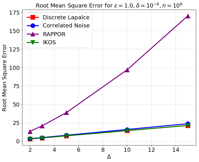
(a) RMSEs for varying $\Delta$

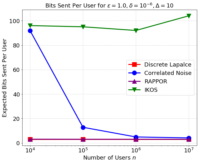
(b) Expected bits sent for varying $n$

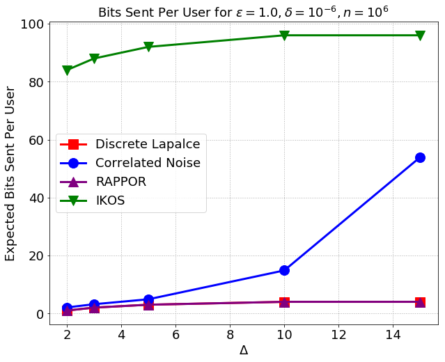
(c) Expected bits sent for varying $\Delta$

Figure 1: Error and communication complexity of our “correlated noise” $\Delta$-summation protocol compared to other protocols.

4.5 Specific Parameter Selection: Proof of Theorem 2

Proof of Theorem 2.

Let $\mathcal{S},\mathbf{C},\mathbf{t}$ be as in Theorem 12, $\varepsilon^{*}=(1-\gamma)\varepsilon,\varepsilon_{1}=\varepsilon_{2}=\min\{1,\gamma\varepsilon\}/2,\delta_{1}=\delta_{2}=\delta/2$, and,

• $\mathcal{D}^{\mathrm{central}}=\operatorname{NB}(1,e^{-\varepsilon^{*}/\Delta})$,

• $\hat{\mathcal{D}}=\operatorname{NB}(\hat{r},\hat{p})$ where $\hat{p}=e^{-0.2\varepsilon_{1}/\Delta}$ and $\hat{r}=3(1+\log(1/\delta_{1}))$,

• $\tilde{\mathcal{D}}^{\mathbf{s}}=\operatorname{NB}(r_{\mathbf{s}},p_{\mathbf{s}})$ where $p_{\mathbf{s}}=e^{-0.2\varepsilon_{2}/(2t_{\mathbf{s}})}$ and $r^{\mathbf{s}}=3(1+\log(|\mathcal{S}|/\delta_{2}))$ for all $\mathbf{s}\in\mathcal{S}$.

From Theorem 10, the $\hat{\mathcal{D}}$-noise addition mechanism is $(\varepsilon_{1},\delta_{1})$-DP for $\Delta$-summation. Corollary 11 implies that the $(\tilde{\mathcal{D}}^{\mathbf{s}})_{\mathbf{s}\in\mathcal{S}}$-noise addition mechanism is $(\varepsilon_{2},\delta_{2})$-DP for $[\mathbf{0}~{}\mathbf{c}_{2}~{}\cdots~{}\mathbf{c}_{\Delta}]$-linear query. As a result, since $\varepsilon^{*}+\varepsilon_{1}+\varepsilon_{2}\leq\varepsilon$ and $\delta_{1}+\delta_{2}=\delta$, Theorem 8 ensures that CorrNoiseCentral with parameters as specified in the theorem is $(\varepsilon,\delta)$-DP.

The error claim follows immediately from 5 together with the fact that $\operatorname{NB}(1,e^{-\varepsilon^{*}/\Delta})-\operatorname{NB}(1,e^{-\varepsilon^{*}}/\Delta)=\operatorname{DLap}(\varepsilon^{*}/\Delta)$. Using 6, we can also bound the expected number of messages as

$$1+\frac{1}{n}\left(2\mathbb{E}[\mathcal{D}^{\mathrm{central}}]+\sum_{\mathbf{s}\in\mathcal{S}}|\mathbf{s}|\cdot\mathbb{E}[\mathcal{D}^{\mathbf{s}}]\right)$$

$$\leq 1+O\left(\frac{\Delta}{\varepsilon^{*}n}\right)+\frac{1}{n}\left(\frac{2\hat{r}}{1-\hat{p}}+\sum_{\mathbf{s}\in\mathcal{S}}\frac{|\mathbf{s}|r_{\mathbf{s}}}{1-p_{\mathbf{s}}}\right)$$

$$=1+O\left(\frac{\Delta\log(1/\delta)}{\gamma\varepsilon n}\right)+O\left(\frac{\|\mathbf{t}\|_{\mathcal{S}}\cdot\log(\Delta/\delta)}{\varepsilon_{2}n}\right)$$

$$\leq 1+O\left(\frac{\Delta\log(1/\delta)}{\gamma\varepsilon n}\right)+O\left(\frac{\Delta\log^{2}\Delta\cdot\log(\Delta/\delta)}{\gamma\varepsilon n}\right),$$

where each message consists of $\lceil\log\Delta\rceil+1$ bits. ∎

5 Experimental Evaluation

We compare our “correlated noise” $\Delta$-summation protocol (Algorithms 1, 2) against known algorithms in the literature, namely the IKOS “split-and-mix” protocol Ishai et al. (2006); Balle et al. (2020); Ghazi et al. (2020c) and the fragmented version of RAPPOR Erlingsson et al. (2014; 2020). We also include the Discrete Laplace mechanism Ghosh et al. (2012) in our plots for comparison, although it is not directly implementable in the shuffle model. We do not include the generalized (i.e., $\Delta$-ary) Randomized Response algorithm Warner (1965) as it always incurs at least as large error as RAPPOR.

For our protocol, we set $\varepsilon^{*}$ in Theorem 8 to $0.9\varepsilon$, meaning that its MSE is that of $\operatorname{DLap}(0.9\varepsilon/\Delta)$. While the parameters set in our proofs give a theoretically vanishing overhead guarantee, they turn out to be rather impractical; instead, we resort to a tighter numerical approach to find the parameters. We discuss this, together with the setting of parameters for the other alternatives, in the SM.

For all mechanisms the root mean square error (RMSE) and the (expected) communication per user only depends on $n,\varepsilon,\delta,\Delta$, and is independent of the input data. We next summarize our findings.

Error.

The IKOS algorithm has the same error as the Discrete Laplace mechanism (in the central model), whereas our algorithm’s error is slightly larger due to $\varepsilon^{*}$ being slightly smaller than $\varepsilon$. On the other hand, the RMSE for RAPPOR grows as $1/\delta$ increases, but it seems to converge as $n$ becomes larger. (For $\delta=10^{-6}$ and $n=10^{4},\dots,10^{7}$, we found that RMSEs differ by less than 1%.)

However, the key takeaway here is that the RMSEs of IKOS, Discrete Laplace, and our algorithm grow only linearly in $\Delta$, but the RMSE of RAPPOR is proportional to $\Theta(\Delta^{3/2})$. This is illustrated in Figure 1(a).

Communication.

While the IKOS protocol achieves the same accuracy as the Discrete Laplace mechanism, it incurs a large communication overhead, as each message sent consists of $\lceil\log(n\Delta)\rceil$ bits and each user needs to send multiple messages. By contrast, when fixing $\Delta$ and taking $n\to\infty$, both RAPPOR and our algorithm only send $1+o(1)$ messages, each of length $\lceil\log\Delta\rceil$ and $\lceil\log\Delta\rceil+1$ respectively. This is illustrated in Figure 1(b). Note that the number of bits sent for IKOS is indeed not a monotone function since, as $n$ increases, the number of messages required decreases but the length of each message increases.

Finally, we demonstrate the effect of varying $\Delta$ in Figure 1(c) for a fixed value of $n$. Although Theorem 2 suggests that the communication overhead should grow roughly linearly with $\Delta$, we have observed larger gaps in the experiments. This seems to stem from the fact that, while the $\tilde{O}(\Delta)$ growth would have been observed if we were using our analytic formula, our tighter parameter computation (detailed in Appendix H.1 of SM) finds a protocol with even smaller communication, suggesting that the actual growth might be less than $\tilde{O}(\Delta)$ though we do not know of a formal proof of this. Unfortunately, for large $\Delta$, the optimization problem for the parameter search gets too demanding and our program does not find a good solution, leading to the “larger gap” observed in the experiments.

6 Conclusions

In this work, we presented a DP protocol for real and $1$-sparse vector aggregation in the shuffle model with accuracy arbitrarily close to the best possible central accuracy, and with relative communication overhead tending to $0$ with increasing number of users. It would be very interesting to generalize our protocol and obtain qualitatively similar guarantees for dense vector summation.

We also point out that in the low privacy regime ($\varepsilon\gg 1$), the staircase mechanism is known to significantly improve upon the Laplace mechanism Geng & Viswanath (2016); Geng et al. (2015); the former achieves MSE that is exponentially small in $\Theta(\varepsilon)$ while the latter has MSE $O(1/\varepsilon^{2})$. An interesting open question is to achieve such a gain in the shuffle model.

Supplementary Material

Appendix A Additional Preliminaries

We start by introducing a few additional notation and lemmas that will be used in our proofs.

Definition 13.

The $\varepsilon$-hockey stick divergence of two (discrete) distributions $\mathcal{D},\mathcal{D}^{\prime}$ is defined as

$$d_{\varepsilon}(\mathcal{D}\|\mathcal{D}^{\prime}):=\sum_{v\in\operatorname{supp}(\mathcal{D})}\left[\Pr_{x\sim\mathcal{D}}[x=v]-e^{\varepsilon}\cdot\Pr_{x\sim\mathcal{D}^{\prime}}[x=v]\right]_{+}$$

where $[y]_{+}:=\max\{y,0\}$.

The following is a (well-known) simple restatement of DP in terms of hockey stick divergence:

Lemma 14.

An algorithm $\mathcal{A}$ is $(\varepsilon,\delta)$-DP iff for any neighboring datasets $X$ and $X^{\prime}$, it holds that $d_{\varepsilon}(\mathcal{A}(X),\mathcal{A}(X^{\prime}))\leq\delta$.

We will also use the following result in (Ghazi et al., 2020b, Lemma 21), which allows us to easily compute differential privacy parameters noise addition algorithms for $\Delta$-summation.

Lemma 15 (Ghazi et al. (2020b)).

An $\mathcal{D}$-noise addition mechanism for $\Delta$-summation is $(\varepsilon,\delta)$-DP iff $d_{\varepsilon}(\mathcal{D}\|k+\mathcal{D})\leq\delta$ for all $k\in\{-\Delta,\dots,+\Delta\}$.

Finally, we will also use the following lemma, which can be viewed as an alternative formulation of the basic composition theorem.

Lemma 16.

Let $\mathcal{D}_{1},\dots,\mathcal{D}_{k},\mathcal{D}^{\prime}_{1},\dots,\mathcal{D}^{\prime}_{k}$ be any distributions and $\varepsilon_{1},\dots,\varepsilon_{k}$ any non-negative real numbers. Then, we have $d_{\varepsilon_{1}+\cdots+\varepsilon_{k}}(\mathcal{D}_{1}\times\cdots\times\mathcal{D}_{k}\|\mathcal{D}^{\prime}_{1}\times\cdots\times\mathcal{D}^{\prime}_{k})\leq\sum_{i\in[k]}d_{\varepsilon_{i}}(\mathcal{D}_{i}\|\mathcal{D}^{\prime}_{i})$.

Appendix B On the Near Optimality of (Discrete) Laplace Mechanism

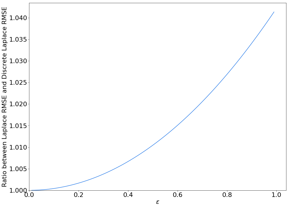
Figure 2: Comparison between RMSE of the Laplace Mechanism and RMSE of the Discrete Laplace Mechanism when varing $\varepsilon$.

In this section, we briefly discuss the near-optimality of Laplace mechanism in the central model. First, we recall that it follows from Ghosh et al. (2012) that the smallest MSE of any $\varepsilon$-DP algorithm (in the central model) for binary summation (i.e., 1-summation) is at least that of the Discrete Laplace mechanism minus a term that converges to zero as $n\to\infty$. In other words, RMSE of the Discrete Laplace mechanism, up to an $o(1)$ additive factor, forms a lower bound for binary summation. Notice that a lower bound on the RMSE for binary summation also yields a lower bound on the RMSE for real summation, since the latter is a more general problem. We plot the comparison between RMSE of the Discrete Laplace mechanism and RMSE of the Laplace mechanism in Figure 2 for $\varepsilon\in[0,1]$. Since the former is a lower bound on RMSE of any $\varepsilon$-DP algorithm for real summation, this plot shows how close the Laplace mechanism is to the lower bound. Specifically, we have found that, in this range of $\varepsilon<1$, the Laplace mechanism is within $5\%$ of the optimal error (assuming $n$ is sufficiently large). Finally, note that our real summation algorithm (Theorem 1) can achieve accuracy arbitrarily close to the Laplace mechanism, and hence our algorithm can also get to within $5\%$ of the optimal error for any $\varepsilon\in[0,1]$.

Appendix C Missing Proofs from Section 3

Below we provide (simple) proofs of the generic form of the error (5) and the communication cost (6) of our protocol.

Proof of 5.

Consider each user $i$. The sum of its output is not affected by the noise from $\mathcal{S}$ since the sum of their messages are zero; in other words, the sum is simply $x_{i}+Z^{+1}_{i}-Z^{-1}_{i}$. As a result, the total error is exactly equal to $\left(\sum_{i\in[n]}Z^{+1}_{i}\right)-\left(\sum_{i\in[n]}Z^{-1}_{i}\right)$. Since each of $Z^{+1}_{i},Z^{-1}_{i}$ is an i.i.d. random variable distributed as $\mathcal{D}^{\mathrm{central}}_{/n}$, the error is distributed as $\mathcal{D}^{\mathrm{central}}-\mathcal{D}^{\mathrm{central}}$. ∎

Proof of 6.

Each user sends at most one message corresponding to its input; in addition to this, the expected number of messages sent in the subsequent steps is equal to

$$\mathbb{E}\left[Z^{+1}_{i}+Z^{-1}_{i}+\sum_{\mathbf{s}\in\mathcal{S}}\sum_{m\in\mathbf{s}}Z^{\mathbf{s}}_{i}\right] =\mathbb{E}[\mathcal{D}^{\mathrm{central}}_{/n}]+\mathbb{E}[\mathcal{D}^{\mathrm{central}}_{/n}]+\sum_{\mathbf{s}\in\mathcal{S}}\sum_{m\in\mathbf{s}}\mathbb{E}[\mathcal{D}^{\mathbf{s}}_{/n}]$$

$$=2\mathbb{E}[\mathcal{D}^{\mathrm{central}}_{/n}]+\sum_{\mathbf{s}\in\mathcal{S}}|\mathbf{s}|\cdot\mathbb{E}[\mathcal{D}^{\mathbf{s}}_{/n}]$$

$$=\frac{1}{n}\left(2\mathbb{E}[\mathcal{D}^{\mathrm{central}}]+\sum_{\mathbf{s}\in\mathcal{S}}|\mathbf{s}|\cdot\mathbb{E}[\mathcal{D}^{\mathbf{s}}]\right)$$

Finally, since each message is a number from $[-\Delta,\Delta]$, it can be represented using $\lceil\log_{2}\Delta\rceil+1$ bits as desired. ∎

Appendix D Missing Proofs from Section 4

D.1 From Shuffle Model to Central Model

Let us restate Algorithm 3 in a slightly different notation where each user’s input $x_{1},\dots,x_{n}$ is represented explicitly in the algorithm (instead of the histogram as in Algorithm 3):

Algorithm 4 Central Algorithm

1:  procedure CorrNoise($x_{1},\dots,x_{n}$)

2:        $u_{-\Delta},\dots,u_{-1}\leftarrow 0$

3:     for $j\in[\Delta]$

4:        $u_{j}\leftarrow|\{i\in[n]\mid x_{i}=j\}|$

5:     Sample $z^{+1}\sim\mathcal{D}^{\mathrm{central}}$

6:     $u_{+1}\leftarrow u_{+1}+Z^{1}$

7:     Sample $z^{-1}\sim\mathcal{D}^{\mathrm{central}}$

8:     $u_{-1}\leftarrow u_{-1}+Z^{-1}$

9:     for $\mathbf{s}\in\mathcal{S}$

10:        Sample $z^{\mathbf{s}}\sim\mathcal{D}^{\mathbf{s}}$

11:        for $m\in\mathbf{s}$

12:           $u_{m}\leftarrow u_{m}+z^{\mathbf{s}}$

13:     return $(u_{-\Delta},\dots,u_{-1},u_{+1},\dots,u_{+\Delta})$.

Observation 17.

CorrNoiseRandomizer is $(\varepsilon,\delta)$-DP in the shuffle model iff CorrNoise is $(\varepsilon,\delta)$-DP in the central model.

Proof.

Consider the analyzer’s view for CorrNoiseRandomizer; all the analyzer sees is a number of messages $-\Delta,\dots,-1,+1,\dots,+\Delta$. Let $u_{i}$ denote the number of messages $i$, for a non-zero integer $i\in[-\Delta,\Delta]$. We will argue that $(u_{-\Delta},\dots,u_{-1},u_{+1},\dots,u_{+\Delta})$ has the same distribution as the output of CorrNoise, from which the observation follows. To see this, notice that the total number of noise atoms $\mathbf{s}$ in CorrNoiseRandomizer across all users is $z^{\mathbf{s}}_{1}+\cdots+z^{\mathbf{s}}_{n}$ which is distributed as $\mathcal{D}^{\mathbf{s}}$. Similarly, the number of additional $-1$ messages and that of $+1$ messages (from Line 5 of CorrNoiseRandomizer) are both distributed as (independent) $\mathcal{D}^{\mathrm{central}}$ random variables. As a result, $(u_{-\Delta},\dots,u_{-1},u_{+1},\dots,u_{+\Delta})$ has the same distribution as the output of CorrNoise. ∎

7 then immediately follows from 17 and the fact that the two algorithms are equivalent.

D.2 Flooding Central Noise: Proof of Lemma 9

Proof of Lemma 9.

Consider any two input neighboring datasets $\mathbf{h},\mathbf{h}^{\prime}$. Let $\varepsilon:=\varepsilon^{*}+\varepsilon_{1}$. From Lemma 14, it suffices to show that $d_{\varepsilon}(\mathcal{M}_{\mathrm{cor}}(\mathbf{h}),\mathcal{M}_{\mathrm{cor}}(\mathbf{h}^{\prime}))\leq\delta_{1}$. Let $\kappa=\left<\mathbf{v},\mathbf{h}\right>-\left<\mathbf{v},\mathbf{h}^{\prime}\right>$; note that by definition of neighboring datasets, we have $-\Delta\leq\kappa\leq\Delta$. We may simplify $d_{\varepsilon}(\mathcal{M}_{\mathrm{cor}}(\mathbf{h}),\mathcal{M}_{\mathrm{cor}}(\mathbf{h}^{\prime}))$ as

$$d_{\varepsilon}(\mathcal{M}_{\mathrm{cor}}(\mathbf{h}),\mathcal{M}_{\mathrm{cor}}(\mathbf{h}^{\prime}))$$

$$=\sum_{a,b\in\mathbb{Z}}\Big{[}\Pr[z^{+1}-z^{-1}+\left<\mathbf{v},\mathbf{h}\right>=a,z^{-1}+\tilde{z}^{-1,+1}=b]-e^{\varepsilon}\Pr[z^{1}-z^{-1}+\left<\mathbf{v},\mathbf{h}^{\prime}\right>=a,z^{-1}+\tilde{z}^{-1,+1}=b]\Big{]}_{+}$$

$$=\sum_{c,b\in\mathbb{Z}}\Big{[}\Pr[z^{+1}-z^{-1}=c-\kappa,z^{-1}+\tilde{z}^{-1,+1}=b]-e^{\varepsilon}\Pr[z^{+1}-z^{-1}=c,z^{-1}+\tilde{z}^{-1,+1}=b]\Big{]}_{+},$$ (1)

where the second equality comes from simply substituting $c=a-\left<\mathbf{v},\mathbf{h}^{\prime}\right>$.

For convenience, let $\lambda_{c}:=\max\{0,\kappa-c\}$. We may expand the first probability above as

$$\Pr[z^{+1}-z^{-1}=c-\kappa,z^{-1}+\tilde{z}^{-1,+1}=b]$$

$$=\sum_{d=\lambda_{c}}^{\infty}\Pr[z^{+1}=c-\kappa+d]\Pr[z^{-1}=d]\Pr[\tilde{z}^{\{-1,+1\}}=b-d].$$ (2)

Similarly, let $\gamma_{c}:=\max\{0,c\}$. We may expand the second probability above as

$$\Pr[z^{+1}-z^{-1}=c,z^{-1}+\tilde{z}^{-1,+1}=b]$$

$$=\sum_{d^{\prime}=\gamma_{c}}^{\infty}\Pr[z^{+1}=c+d^{\prime}]\Pr[z^{-1}=d^{\prime}]\Pr[\tilde{z}^{\{-1,+1\}}=b-d^{\prime}]$$

$$=\sum_{d=\lambda_{c}}^{\infty}\Pr[z^{+1}=c+d-(\lambda_{c}-\gamma_{c})]\Pr[z^{-1}=d-(\lambda_{c}-\gamma_{c})]\Pr[\tilde{z}^{\{-1,+1\}}=b-d+(\lambda_{c}-\gamma_{c})].$$ (3)

Next, notice that for $d\geq\lambda_{c}$, we have

$$\frac{\Pr[z^{+1}=c+d-(\lambda_{c}-\gamma_{c})]\Pr[z^{-1}=d-(\lambda_{c}-\gamma_{c})]}{\Pr[z^{+1}=c-\kappa+d]\Pr[z^{-1}=d]}$$

$$=\frac{\exp\left(-\frac{\varepsilon^{*}}{\Delta}(c+d-(\lambda_{c}-\gamma_{c}))\right)\exp\left(-\frac{\varepsilon^{*}}{\Delta}(d-(\lambda_{c}-\gamma_{c}))\right)}{\exp\left(-\frac{\varepsilon^{*}}{\Delta}(c-\kappa+d)\right)\exp\left(-\frac{\varepsilon^{*}}{\Delta}(d)\right)}$$

$$=\exp\left(-\frac{\varepsilon^{*}}{\Delta}(\kappa-2(\lambda_{c}-\gamma_{c}))\right)$$

$$\geq\exp(-\varepsilon^{*}),$$

where the last inequality employs a simple observation that $(\lambda_{c}-\gamma_{c})\leq\kappa\leq\Delta$.

Plugging the above back into (3), we get

$$\Pr[z^{+1}-z^{-1}=c,z^{-1}+\tilde{z}^{-1,+1}=b]$$ (4)

$$\geq e^{-\varepsilon^{*}}\cdot\sum_{d=\lambda_{c}}^{\infty}\Pr[z^{+1}=c-\kappa+d]\Pr[z^{-1}=d]\Pr[\tilde{z}^{\{-1,+1\}}=b-d+(\lambda_{c}-\gamma_{c})].$$ (5)

Then, plugging both (2) and (5) into (1), we arrive at

$$d_{\varepsilon}(\mathcal{M}_{\mathrm{cor}}(\mathbf{h}),\mathcal{M}_{\mathrm{cor}}(\mathbf{h}^{\prime}))$$

$$\leq\sum_{c,b\in\mathbb{Z}}\left[\sum_{d=\lambda_{c}}^{\infty}\Pr[z^{+1}=c-\kappa+d]\Pr[z^{-1}=d]\right.$$

$$\qquad\qquad\left(\Pr[\tilde{z}^{\{-1,+1\}}=b-d]-e^{\varepsilon_{1}}\Pr[\tilde{z}^{\{-1,+1\}}=b-d+(\lambda_{c}-\gamma_{c})]\right)\Bigg{]}_{+}$$

$$\leq\sum_{c,b\in\mathbb{Z}}\sum_{d=\lambda_{c}}^{\infty}\Pr[z^{+1}=c-\kappa+d]\Pr[z^{-1}=d]$$

$$\qquad\qquad\cdot\left[\Pr[\tilde{z}^{\{-1,+1\}}=b-d]-e^{\varepsilon_{1}}\Pr[\tilde{z}^{\{-1,+1\}}=b-d+(\lambda_{c}-\gamma_{c})]\right]_{+}$$

$$=\sum_{c\in\mathbb{Z}}\sum_{d=\lambda_{c}}^{\infty}\Pr[z^{+1}=c-\kappa+d]\Pr[z^{-1}=d]$$

$$\qquad\qquad\left(\sum_{b\in\mathbb{Z}}\left[\Pr[\tilde{z}^{\{-1,+1\}}=b-d]-e^{\varepsilon_{1}}\Pr[\tilde{z}^{\{-1,+1\}}=b-d+(\lambda_{c}-\gamma_{c})]\right]_{+}\right)$$

$$=\sum_{c\in\mathbb{Z}}\sum_{d=\lambda_{c}}^{\infty}\Pr[z^{+1}=c-\kappa+d]\Pr[z^{-1}=d]\cdot d_{\varepsilon_{1}}(\hat{\mathcal{D}}\|\hat{\mathcal{D}}+(\gamma_{c}-\lambda_{c})).$$

Now, recall that $|\gamma_{c}-\lambda_{c}|\leq|\kappa|\leq\Delta$. Thus, from our assumption that the $\hat{\mathcal{D}}$-mechanism is $(\varepsilon_{1},\delta_{1})$-DP for $\Delta$-summation and Lemma 15, we can conclude that $d_{\varepsilon_{1}}(\hat{\mathcal{D}}\|\hat{\mathcal{D}}+(\gamma_{c}-\lambda_{c}))\leq\delta_{1}$. Hence, we can further bound $d_{\varepsilon}(\mathcal{M}_{\mathrm{cor}}(\mathbf{h}),\mathcal{M}_{\mathrm{cor}}(\mathbf{h}^{\prime}))$ as

$$d_{\varepsilon}(\mathcal{M}_{\mathrm{cor}}(\mathbf{h}),\mathcal{M}_{\mathrm{cor}}(\mathbf{h}^{\prime}))\leq\delta_{1}\cdot\left(\sum_{c\in\mathbb{Z}}\sum_{d=\lambda_{c}}^{\infty}\Pr[z^{+1}=c-\kappa+d]\Pr[z^{-1}=d]\right)=\delta_{1}.$$

This implies that $\mathcal{M}_{\mathrm{cor}}$ is $(\varepsilon^{*}+\varepsilon_{1},\delta_{1})$-DP as desired. ∎

D.3 Finding a Right Inverse: Proof of Theorem 12

Proof of Theorem 12.

We first select $\mathcal{S}$ to be the collection $\{-1,+1\}$ and all multisets of the form $\{i,-\lfloor i/2\rfloor,-\lceil i/2\rceil\}$ for all $i\in\{-\Delta,\dots,-2,+2,\dots,+\Delta\}$.

Throughout this proof, we write $\mathbf{c}_{i}$ to denote the $i$th column of $\mathbf{C}$. We construct a right inverse $\mathbf{C}$ by constructing its columns iteratively as follows:

• First, we let $\mathbf{c}_{-1}=\mathbf{1}_{\{-1,+1\}}$ denote the indicator vector of coordinate $\mathbf{s}=\{-1,+1\}$.

• For convenience, we let $\mathbf{c}_{1}=\mathbf{0}$ although this column is not present in the final matrix $\mathbf{C}$.

• For each $i\in\{2,\dots,\Delta\}$:

  • Let $i_{1}=\lfloor i/2\rfloor$ and $i_{2}=\lceil i/2\rceil$.

  • Let $\mathbf{c}_{i}$ be $\mathbf{1}_{\{i,-i_{1},-i_{2}\}}-\mathbf{c}_{-i_{1}}-\mathbf{c}_{-i_{2}}$.

  • Let $\mathbf{c}_{-i}$ be $\mathbf{1}_{\{-i,i_{1},i_{2}\}}-\mathbf{c}_{i_{1}}-\mathbf{c}_{i_{2}}$.

We will now show by induction that $\mathbf{C}$ as constructed above indeed satisfies $\tilde{\mathbf{A}}\mathbf{C}=\mathbf{I}$. Let $\tilde{\mathbf{A}}_{i,*}$ denote the $i$th row of $\tilde{\mathbf{A}}$. Equivalently, we would like to show that

$$\tilde{\mathbf{A}}_{i^{\prime},*}\mathbf{c}_{i}=\mathbf{1}[i^{\prime}=i],$$ (6)

for all $[-\Delta,\Delta]_{-1}$. We will prove this by induction on $|i|$.

(Base Case)

We will show that this holds for $i=-1$. Since $\mathbf{c}_{1}=\mathbf{1}_{\{-1,1\}}$, we have

$$\tilde{\mathbf{A}}_{i^{\prime},*}\mathbf{c}_{i}=\tilde{\mathbf{A}}_{i,\{-1,1\}}=\mathbf{1}[i\in\{-1,1\}]=\mathbf{1}[i=-1].$$

(Inductive Step)

Now, suppose that (6) holds for all $i$ such that $|i|<m$ for some $m\in\mathbb{N}\setminus\{1\}$. We will now show that it holds for $i=m,-m$ as well. Let $m_{1}=\lfloor m/2\rfloor$ and $m_{2}=\lceil m/2\rceil$. For $i=m$, let $\mathbf{s}=\{m,-m_{1},-m_{2}\}$; we have

$$\mathbf{A}_{i^{\prime},*}\mathbf{c}_{i} =\mathbf{A}_{i^{\prime},*}\left(\mathbf{1}_{\mathbf{s}}-\mathbf{c}_{-m_{1}}-\mathbf{c}_{-m_{2}}\right)$$

(From inductive hypothesis) $$=\mathbf{A}_{i^{\prime},*}\mathbf{1}_{\mathbf{s}}-\mathbf{1}[i^{\prime}=-m_{1}]-\mathbf{1}[i^{\prime}=-m_{2}]$$

$$=\mathbf{s}_{i^{\prime}}-\mathbf{1}[i^{\prime}=-m_{1}]-\mathbf{1}[i^{\prime}=-m_{2}]$$

$$=\mathbf{1}[i=i^{\prime}],$$

where the last inequality follows from the definition of $\mathbf{s}$.

The case where $i=-m$ is similar. Specifically, letting $\mathbf{s}=\{-m,m_{1},m_{2}\}$, we have

$$\mathbf{A}_{i^{\prime},*}\mathbf{c}_{i} =\mathbf{A}_{i^{\prime},*}\left(\mathbf{1}_{\mathbf{s}}-\mathbf{c}_{m_{1}}-\mathbf{c}_{m_{2}}\right)$$

(From inductive hypothesis) $$=\mathbf{A}_{i^{\prime},*}\mathbf{1}_{\mathbf{s}}-\mathbf{1}[i^{\prime}=m_{1}]-\mathbf{1}[i^{\prime}=m_{2}]$$

$$=\mathbf{s}_{i^{\prime}}-\mathbf{1}[i^{\prime}=m_{1}]-\mathbf{1}[i^{\prime}=m_{2}]$$

$$=\mathbf{1}[i=i^{\prime}].$$

Let $\Gamma=\Delta\cdot\lceil 1+\log\Delta\rceil$. Let $\mathbf{t}\in\mathbb{Z}^{\mathcal{S}}$ be defined by

$$\mathbf{t}_{\mathbf{s}}=\begin{cases}\Gamma&\text{ if }\mathbf{s}=\{-1,1\}\\ \lceil\Gamma/m\rceil&\text{ if }\mathbf{s}=\{m,-\lceil m/2\rceil,-\lfloor m/2\rfloor\}\text{ or }\mathbf{s}=\{-m,\lceil m/2\rceil,\lfloor m/2\rfloor\}\text{ for some }m\in\{2,\dots,\Delta\}.\end{cases}$$

Since $\|\mathbf{s}\|_{1}\leq 3$ for all $\mathbf{s}\in\mathcal{S}$, we have

$$\|\mathbf{t}\|_{\mathcal{S}}\leq 3\cdot\|\mathbf{t}\|_{1}=\Gamma+\sum_{m=2,\dots,\Delta}\lceil\Gamma/m\rceil=\Gamma\cdot O(\log\Delta)=O(\Delta\log^{2}\Delta),$$

as desired.

Finally, we will show via induction on $|i|$ that

$$\sum_{\mathbf{s}\in\mathcal{S}}\frac{|\mathbf{C}_{\mathbf{s},i}|}{\mathbf{t}_{\mathbf{s}}}\leq\frac{|i|\cdot\lceil 1+\log|i|\rceil}{\Gamma},$$ (7)

which, from our choice of $\Gamma$, implies the last property.

(Base Case)

We have

$$\sum_{\mathbf{s}\in\mathcal{S}}\frac{|\mathbf{C}_{\mathbf{s},-1}|}{\mathbf{t}_{\mathbf{s}}}=\frac{1}{\mathbf{t}_{\{-1,+1\}}}=\frac{1}{\Gamma}.$$

(Inductive Step)

For convenience, in the derivation below, we think of $\mathbf{C}_{\mathbf{s},1}$ as 0 for all $\mathbf{s}\in\mathcal{S}$; note that in fact, row $1$ does not exist for $\mathbf{C}$.

Suppose that (7) holds for all $i\in[-\Delta,\Delta]_{-1}$ such that $|i|<m$ for some $m\in\mathbb{N}\setminus\{1\}$. Now, consider $i=m$; letting $m_{1}=\lceil m/2\rceil,m_{2}=\lfloor m/2\rfloor$from the definition of $\mathbf{c}_{i}$, we have

$$\sum_{\mathbf{s}\in\mathcal{S}}\frac{|\mathbf{C}_{\mathbf{s},i}|}{\mathbf{t}_{\mathbf{s}}} \leq\frac{1}{\mathbf{t}_{\{m,-m_{1},-m_{2}\}}}+\sum_{\mathbf{s}\in\mathcal{S}}\frac{|\mathbf{C}_{\mathbf{s},m_{1}}|}{\mathbf{t}_{\mathbf{s}}}+\sum_{\mathbf{s}\in\mathcal{S}}\frac{|\mathbf{C}_{\mathbf{s},m_{2}}|}{\mathbf{t}_{\mathbf{s}}}$$

$$(\text{From inductive hypothesis}) \leq\frac{1}{\mathbf{t}_{\{m,-m_{1},-m_{2}\}}}+\frac{m_{1}\lceil 1+\log m_{1}\rceil}{\Gamma}+\frac{m_{2}\lceil 1+\log m_{2}\rceil}{\Gamma}$$

$$\leq\frac{1}{\mathbf{t}_{\{m,-m_{1},-m_{2}\}}}+\frac{m_{1}\lceil\log m\rceil}{\Gamma}+\frac{m_{2}\lceil\log m\rceil}{\Gamma}$$

$$=\frac{1}{\mathbf{t}_{\{m,-m_{1},-m_{2}\}}}+\frac{m\lceil\log m\rceil}{\Gamma}$$

$$(\text{From our choice of }\mathbf{t}_{\{m,-m_{1},-m_{2}\}}) \leq\frac{m}{\Gamma}+\frac{m\lceil\log m\rceil}{\Gamma}$$

$$=\frac{m\lceil 1+\log m\rceil}{\Gamma}.$$

Similarly, for $i=-m$, we have

$$\sum_{\mathbf{s}\in\mathcal{S}}\frac{|\mathbf{C}_{\mathbf{s},i}|}{\mathbf{t}_{\mathbf{s}}} \leq\frac{1}{\mathbf{t}_{\{-m,m_{1},m_{2}\}}}+\sum_{\mathbf{s}\in\mathcal{S}}\frac{|\mathbf{C}_{\mathbf{s},-m_{1}}|}{\mathbf{t}_{\mathbf{s}}}+\sum_{\mathbf{s}\in\mathcal{S}}\frac{|\mathbf{C}_{\mathbf{s},-m_{2}}|}{\mathbf{t}_{\mathbf{s}}}$$

$$(\text{From inductive hypothesis}) \leq\frac{1}{\mathbf{t}_{\{-m,m_{1},m_{2}\}}}+\frac{m_{1}\lceil 1+\log m_{1}\rceil}{\Gamma}+\frac{m_{2}\lceil 1+\log m_{2}\rceil}{\Gamma}$$

$$\leq\frac{1}{\mathbf{t}_{\{-m,m_{1},m_{2}\}}}+\frac{m_{1}\lceil\log m\rceil}{\Gamma}+\frac{m_{2}\lceil\log m\rceil}{\Gamma}$$

$$=\frac{1}{\mathbf{t}_{\{-m,m_{1},m_{2}\}}}+\frac{m\lceil\log m\rceil}{\Gamma}$$

$$(\text{From our choice of }\mathbf{t}_{\{-m,m_{1},m_{2}\}}) \leq\frac{m}{\Gamma}+\frac{m\lceil\log m\rceil}{\Gamma}$$

$$=\frac{m\lceil 1+\log m\rceil}{\Gamma}.\qed$$

D.4 Negative Binomial Mechanism for Linear Queries: Proof of Corollary 11

Proof of Corollary 11.

We denote the $(\mathcal{D}^{i})_{i\in\mathcal{I}}$-noise addition mechanism by $\mathcal{M}$. Furthermore, we write $\mathbfcal{D}$ to denote the noise distribution (i.e., distribution of $\mathbf{z}$ where $z_{i}\sim\mathcal{D}^{i}$).

Consider two neighboring datasets $\mathbf{h},\mathbf{h}^{\prime}$. We have

$$d_{\varepsilon}(\mathcal{M}(\mathbf{h})\|\mathcal{M}(\mathbf{h}^{\prime})) =d_{\varepsilon}\left(\mathbf{Q}\mathbf{h}+\mathbfcal{D}\middle\|\mathbf{Q}\mathbf{h}^{\prime}+\mathbfcal{D}\right)$$

$$=d_{\varepsilon}\left(\mathbfcal{D}\|\mathbf{Q}(\mathbf{h}^{\prime}-\mathbf{h})+\mathbfcal{D}\right)$$

$$=d_{\varepsilon}\left(\prod_{i\in\mathcal{I}}\mathcal{D}^{i}\middle\|\prod_{i\in\mathcal{I}}((\mathbf{Q}(\mathbf{h}^{\prime}-\mathbf{h}))_{i}+\mathcal{D}^{i})\right).$$

Now, notice that $\mathbf{Q}(\mathbf{h}^{\prime}-\mathbf{h})$ is dominated by $2\mathbf{t}$. Let $\varepsilon_{i}:=\varepsilon\cdot\frac{|(\mathbf{Q}(\mathbf{h}^{\prime}-\mathbf{h}))_{i}|}{2\mathbf{t}_{i}}$ for all $i\in\mathcal{I}$; we have $\sum_{i\in\mathcal{I}}\varepsilon_{i}\leq\varepsilon$. As a result, applying Lemma 16, we get

$$d_{\varepsilon}(\mathcal{M}(\mathbf{h})\|\mathcal{M}(\mathbf{h}^{\prime})) \leq\sum_{i\in\mathcal{I}}d_{\varepsilon_{i}}(\mathcal{D}^{i}\|(\mathbf{Q}(\mathbf{h}^{\prime}-\mathbf{h}))_{i}+\mathcal{D}^{i})$$

$$(\text{From \lx@cref{creftypecap~refnum}{thm:nb-scalar} and our choice of }\varepsilon_{i},p_{i},r_{i}) \leq\sum_{i\in\mathcal{I}}\delta/|\mathcal{I}|$$

$$=\delta,$$

which concludes our proof. ∎

D.5 From Integers to Real Numbers: Proof of Theorem 1

We now prove Theorem 1. The proof follows the discretization via randomized rounding of Balle et al. (2020).

Proof of Theorem 1.

The algorithm for real summation works as follows:

• Let $\Delta=\lceil\frac{\varepsilon}{2}\cdot\sqrt{n/\zeta}\rceil$.

• Each user randomly round the input $x_{i}\in[0,1]$ to $y_{i}\in\{0,\dots,\Delta\}$ such that

  $$y_{i}=\begin{cases}\lfloor x_{i}\Delta\rfloor&\text{ with probability }1-(x_{i}-\lfloor x_{i}\Delta\rfloor),\\ \lfloor x_{i}\Delta\rfloor+1&\text{ with probability }x_{i}-\lfloor x_{i}\Delta\rfloor.\\ \end{cases}$$

• Run $\Delta$-summation algorithm from Theorem 2 on the inputs $y_{1},\dots,y_{n}$ with $\gamma=\zeta/2$ to get an estimated sum $s$.

• Output $s/\Delta$.

Using the communication guarantee of Theorem 2, we can conclude that, in the above algorithm, each user sends

$$1+\left(\frac{\Delta}{\gamma\varepsilon n}\right)\cdot O\left(\log(1/\delta)+\log^{2}\Delta\cdot\log(\Delta/\delta)\right)=1+\left(\frac{1}{\zeta\sqrt{\zeta n}}\right)O\left(\log(1/\delta)+\log^{2}(n/\zeta)\cdot\log(n/(\zeta\delta))\right)$$

messages in expectation and that each message contains

$$\lceil\log\Delta\rceil+1=\left\lceil\log\left(\frac{\varepsilon}{2}\cdot\sqrt{n/\zeta}\right)\right\rceil+1\leq 0.5(\log n+\log(1/\zeta))+O(1)$$

bits.

We will next analyze the MSE of the protocol. As guaranteed by Theorem 2, $s$ can be written as $y_{1}+\cdots+y_{n}+e$ where $e$ is distributed as $\operatorname{DLap}((1-\gamma)\varepsilon/\Delta)$. Since $e,\Delta x_{1}-y_{1},\dots,\Delta x_{n}-y_{n}$ are all independent and have zero mean, the MSE can be rearranged as

$$\mathbb{E}[(x_{1}+\cdots+x_{n}-s/\Delta)^{2}] =\frac{1}{\Delta^{2}}\cdot\mathbb{E}[((\Delta x_{1}-y_{1})+\cdots+(\Delta x_{n}-y_{n})-e)^{2}]$$

$$=\frac{1}{\Delta^{2}}\left(\mathbb{E}[e^{2}]+\sum_{i=1}^{n}\mathbb{E}[(\Delta x_{i}-y_{i})^{2}]\right).$$

Recall that $\mathbb{E}[e^{2}]$ is simply the variance of the discrete Laplace distribution with parameter $(1-\gamma)\varepsilon/\Delta$, which is at most $\frac{2\Delta^{2}}{(1-\gamma)^{2}\varepsilon^{2}}$. Moreover, for each $i$, $\mathbb{E}[(\Delta x_{i}-y_{i})^{2}]=(x_{i}-\lfloor x_{i}\Delta\rfloor)(1-(x_{i}-\lfloor x_{i}\Delta\rfloor))\leq 1/4$. Plugging this to the above equality, we have

$$\mathbb{E}[(x_{1}+\cdots+x_{n}-s/\Delta)^{2}]=\frac{1}{\Delta^{2}}\left(\frac{2\Delta^{2}}{(1-\gamma)^{2}\varepsilon^{2}}+\frac{n}{4}\right)\leq\frac{2}{(1-\zeta)^{2}\varepsilon^{2}},$$

where the inequality follows from our parameter selection. The right hand side of the above inequality is indeed the MSE of Laplace mechanism with parameter $(1-\zeta)\varepsilon$. This concludes our proof. ∎

Appendix E From Real Summation to 1-Sparse Vector Summation: Proof of Corollary 3

In this section, we prove our result for 1-Sparse Vector Summation (Corollary 3). The idea, formalized below, is to run our real-summation randomizer in each coordinate independently.

Proof of Corollary 3.

Let $v^{i}\in\mathbb{R}^{d}$ denote the (1-sparse) vector input to the $i$th user. The randomizer simply runs the real summation randomizer on each coordinate of $v^{i}$, which gives the messages to send. It then attaches to each message the coordinate, as to distinguish the different coordinates. We stress that the randomizer for each coordinate is run with privacy parameters $(\varepsilon/2,\delta/2)$ instead of $(\varepsilon,\delta)$.

Algorithm 5 1-Sparse Vector Randomizer

1:  procedure SparseVectorCorrNoiseRandomizer${}_{n}(v^{i})$

2:     for $j\in[d]$

3:        $S_{j}\leftarrow\textsc{CorrNoiseRandomizer}^{\varepsilon/2,\delta/2}(v^{i}_{j})$

4:        for $m\in S_{j}$

5:           Send $(i,m)$

The analyzer simply separates the messages based on the coordinates attached to them. Once this is done, messages corresponding to each coordinate are then plugged into the real summation randomizer (that just sums them up), which gives us the estimate of that coordinate. (Note that, similar to $R$, each $R_{j}$ is a multiset.)

Algorithm 6 1-Sparse Vector Randomizer

1:  procedure SparseVectorCorrNoiseAnalyzer

2:     $R\leftarrow$ multiset of messages received

3:     for $j\in[d]$

4:        $R_{j}\leftarrow\{m\mid(j,m)\in R_{j}\}$

5:     return $(\textsc{CorrNoiseAnalyzer}(R_{1}),\dots,\textsc{CorrNoiseAnalyzer}(R_{d}))$

The accuracy claim follows trivially from that of the real summation accuracy in Theorem 1 with $(\varepsilon/2,\delta/2)$-DP. In terms of the communication complexity, since $v^{i}$ is non-zero in only one coordinate and that the expected number of messages sent for CorrNoiseRandomizer with zero input is only $\tilde{O}_{\zeta,\varepsilon}\left(\frac{\log(1/\delta)}{\sqrt{n}}\right)$, the total expected number of messages sent by SparseVectorCorrNoiseRandomizer is

$$1+d\cdot\tilde{O}_{\zeta,\varepsilon}\left(\frac{\log(1/\delta)}{\sqrt{n}}\right)$$

as desired. Furthermore, each message is the real summation message, which consists of only $\tfrac{1}{2}\log n+O(\log\frac{1}{\zeta})$ bits, appended with a coordinate, which can be represented in $\lceil\log d\rceil$ bits. Hence, the total number of bits required to represent each message of SparseVectorCorrNoiseRandomizer is $\log{d}+\tfrac{1}{2}\log n+O(\log\frac{1}{\zeta})$.

We will finally prove that the algorithm is $(\varepsilon/2,\delta/2)$-DP. Consider any two neighboring input datasets $X=(v_{1},\dots,v_{n})$ and $X^{\prime}=(v_{1},\dots,v_{n-1},v^{\prime}_{n})$ that differs only on the last user’s input. Let $J\subseteq[d]$ denote the set of coordinates that $v_{n},v^{\prime}_{n}$ differ on. Since $v_{n},v^{\prime}_{n}$ are both 1-sparse, we can conclude that $|J|\leq 2$. Notice that the view of the analyzer is $R_{1},\dots,R_{d}$; let $\mathcal{D}_{1},\dots,\mathcal{D}_{d}$ be the distributions of $R_{1},\dots,R_{d}$ respectively for the input dataset $X$, and $\mathcal{D}^{\prime}_{1},\dots,\mathcal{D}^{\prime}_{d}$ be the respective distributions for the input dataset $X^{\prime}$. We have

$$d_{\varepsilon}(\mathcal{D}_{1}\times\cdots\times\mathcal{D}_{d}\|\mathcal{D}^{\prime}_{1}\times\cdots\times\mathcal{D}^{\prime}_{d}) =d_{\varepsilon}\left(\prod_{j\in J}\mathcal{D}_{j}\middle\|\prod_{j\in J}\mathcal{D}^{\prime}_{j}\right)$$

$$(\text{From \lx@cref{creftypecap~refnum}{lem:basic-composition-hockeystick} and }|J|\leq 2) \leq\sum_{j\in J}d_{\varepsilon/2}\left(\mathcal{D}_{j}\|\mathcal{D}^{\prime}_{j}\right)$$

$$(\text{Since {CorrNoiseRandomizer}\ is }(\varepsilon/2,\delta/2)\text{-DP}) \leq\sum_{i\in J}\delta/2$$

$$\leq\delta.$$

From this and since $R_{1},\dots,R_{d}$ are independent, we can conclude that the algorithm is $(\varepsilon,\delta)$-DP as claimed. ∎

Appendix F Concrete Parameter Computations

In this section, we describe modifications to the above proofs that result in a more practical set of parameters. As explained in the next section, these are used in our experiments to get a smaller amount of noise than the analytic bounds.

F.1 Tight Bound for Matrix-Specified Linear Queries

By following the definition of differential privacy, one can arrive at a compact description of when the mechanism is differentially private:

Lemma 18.

The $\mathbfcal{D}$-noise addition mechanism is $(\varepsilon,\delta)$-DP for $\mathbf{Q}$-linear query problem if the following holds for every pair of columns $j,j^{\prime}\in[\Delta]$ of $\mathbf{Q}$:

$$d_{\varepsilon}\left(\prod_{i\in\mathcal{I}}(\mathcal{D}^{i}+Q_{i,j}-Q_{i,j^{\prime}})\middle\|\prod_{i\in\mathcal{I}}\mathcal{D}^{i}\right)\leq\delta.$$

Proof.

This follows from the fact that the output distribution is $\prod_{i\in\mathcal{I}}(\mathcal{D}^{i}+\mathbf{Q}_{i,*}\mathbf{h})$, $d_{\varepsilon}$ is shift-invariant, and Lemma 14. ∎

Plugging the above into the negative binomial mechanism, we get:

Lemma 19.

Suppose that $\mathcal{D}^{i}=\operatorname{NB}(r_{i},p_{i})$ for each $i\in\mathcal{I}$. The $(\mathcal{D}^{i})_{\mathcal{I}}$-mechanism is $(\varepsilon,\delta)$-DP for $\mathbf{Q}$-linear query problem if the following holds for every pair of columns $i,i^{\prime}\in[q]$ of $\mathbf{Q}$:

$$d_{\varepsilon}\left(\prod_{i\in\mathcal{I}}(\operatorname{NB}(r_{i},p_{i})+\mathbf{Q}_{i,j}-\mathbf{Q}_{i,j^{\prime}})\middle\|\prod_{i\in\mathcal{I}}\operatorname{NB}(r_{i},p_{i})\right)\leq\delta.$$

Appendix G Refined Analytic Bounds

We use the following analytic bound, which is a more refined version of Corollary 11. Notice below that we may select $\mathbf{t}^{\prime}=2\mathbf{t}$ where $\mathbf{t}$ is as in Corollary 11 and satisfies the requirement. However, the following bound allows us greater flexibility in choosing $\mathbf{t}^{\prime}$. By optimizing for $\mathbf{t}^{\prime}$, we get 30-50% reduction in the noise magnitude compared to using Corollary 11 together with the explicitly constructed $\mathbf{t}$ from the proof of Theorem 12.

Lemma 20.

Suppose that, for every pair of columns $\mathbf{q}_{j},\mathbf{q}_{j^{\prime}}$ of $\mathbf{Q}\in\mathbb{Z}^{\mathcal{I}\times[\Delta]}$, $\mathbf{q}_{j}-\mathbf{q}_{j^{\prime}}$ is dominated by $\mathbf{t}^{\prime}\in\mathbb{R}^{\mathcal{I}}_{+}$. For each $i\in\mathcal{I}$, let $p_{i}=e^{-0.2\varepsilon/t^{\prime}_{i})}$, $r_{i}=3(1+\log(|\mathcal{I}|/\delta))$ and $\mathcal{D}^{i}=\operatorname{NB}(r_{i},p_{i})$. Then, $(\mathcal{D}^{i})_{i\in\mathcal{I}}$-noise addition mechanism is $(\varepsilon,\delta)$-DP for $\mathbf{Q}$-linear query.

Proof.

We denote the $(\mathcal{D}^{i})_{i\in\mathcal{I}}$-noise addition mechanism by $\mathcal{M}$. Furthermore, we write $\mathbfcal{D}$ to denote the noise distribution (i.e., distribution of $\mathbf{z}$ where $z_{i}\sim\mathcal{D}^{i}$).

Consider two neighboring datasets $\mathbf{h},\mathbf{h}^{\prime}$. We have

$$d_{\varepsilon}(\mathcal{M}(\mathbf{h})\|\mathcal{M}(\mathbf{h}^{\prime})) =d_{\varepsilon}\left(\mathbf{Q}\mathbf{h}+\mathbfcal{D}\middle\|\mathbf{Q}\mathbf{h}^{\prime}+\mathbfcal{D}\right)$$

$$=d_{\varepsilon}\left(\mathbfcal{D}\|\mathbf{Q}(\mathbf{h}^{\prime}-\mathbf{h})+\mathbfcal{D}\right)$$

$$=d_{\varepsilon}\left(\prod_{i\in\mathcal{I}}\mathcal{D}^{i}\middle\|\prod_{i\in\mathcal{I}}((\mathbf{Q}(\mathbf{h}^{\prime}-\mathbf{h}))_{i}+\mathcal{D}^{i})\right).$$

Now, notice that our assumption implies that $\mathbf{Q}(\mathbf{h}^{\prime}-\mathbf{h})$ is dominated by $\mathbf{t}^{\prime}$. Let $\varepsilon_{i}:=\varepsilon\cdot\frac{|(\mathbf{Q}(\mathbf{h}^{\prime}-\mathbf{h}))_{i}|}{t^{\prime}_{i}}$ for all $i\in\mathcal{I}$; we have $\sum_{i\in\mathcal{I}}\varepsilon_{i}\leq\varepsilon$. As a result, applying Lemma 16, we get

$$d_{\varepsilon}(\mathcal{M}(\mathbf{h})\|\mathcal{M}(\mathbf{h}^{\prime})) \leq\sum_{i\in\mathcal{I}}d_{\varepsilon_{i}}(\mathcal{D}^{i}\|(\mathbf{Q}(\mathbf{h}^{\prime}-\mathbf{h}))_{i}+\mathcal{D}^{i})$$

$$(\text{From \lx@cref{creftypecap~refnum}{thm:nb-scalar} and our choice of }\varepsilon_{i},p_{i},r_{i}) \leq\sum_{i\in\mathcal{I}}\delta/|\mathcal{I}|$$

$$=\delta,$$

which concludes our proof. ∎

Appendix H Experimental Evaluation: Additional Details and Results

In this section, we give additional details on how to set the parameters and provide additional experimental results, including the effects of $\varepsilon,\delta$ on the $\Delta$-summation protocols and an experiment on the real summation problem on a census dataset.

H.1 Noise parameter settings.

Our Correlated Noise Protocol.

Recall that the notions of $\mathcal{D}^{\mathrm{central}},\hat{\mathcal{D}},\tilde{\mathcal{D}}^{\mathbf{s}},\varepsilon^{*},\varepsilon_{1},\varepsilon_{2},\delta_{1},\delta_{2}$ from Theorem 2. We always set $\varepsilon^{*}$ beforehand: in the $\Delta$-summation experiments (where the entire errors come from the Discrete Laplace noises), $\varepsilon^{*}$ is set to be $0.9\varepsilon$ as to minimize the noise. On the other hand, for real summation experiments where most of the errors are from discretization, we set $\varepsilon^{*}$ to be $0.1\varepsilon$; this is also to help reduce the number of messages as there is now more privacy budget allocated for the $\hat{\mathcal{D}}$ and $\tilde{\mathcal{D}}^{\mathbf{s}}$ noise. Once $\varepsilon^{*}$ is set, we split the remaining $\varepsilon-\varepsilon^{*}$ among $\varepsilon_{1}$ and $\varepsilon_{2}$; we give between 50% and 90% to $\varepsilon_{1}$ depending on the other parameters, so as to minimize the number of messages.

Once the privacy budget is split, we first use Lemma 20 to set $\hat{\mathcal{D}}=\operatorname{NB}(\hat{r},\hat{p}),\tilde{\mathcal{D}}^{\mathbf{s}}=\operatorname{NB}(r^{\mathbf{s}},p^{\mathbf{s}})$; the latter also involves an optimization problem over $\mathbf{t}^{\prime}$, which turns out to be solvable in a relatively short amount of time for moderate values of $\Delta$. This gives us the “initial” parameters for $\mathbf{r},\hat{p},r^{\mathbf{s}},p^{\mathbf{s}}$. We then formulate a generic optimization problem, together with the condition in Lemma 19, and use it to further search for improved parameters. This last search for parameters works well for small values of $\Delta$ and results in as much as $40-80\%$ reduction in the expected number of messages. However, as $\Delta$ grows, this gain becomes smaller since the number of parameters grows linearly with $\Delta$ and the condition in Lemma 19 also takes more resources to compute; thus, the search algorithm fails to yield parameters significantly better than the initial parameters.

Fragmented RAPPOR.

We use the same approach as Ghazi et al. (2020b) to set the parameter (i.e., flip probability) of Fragmented RAPPOR. At a high level, we set a parameter in an “optimistic” manner, meaning that the error and expected number of messages reported might be even lower than the true flip probability that is $(\varepsilon,\delta)$-DP. Roughly speaking, when we would like to check whether a flip probability is feasible, we take two explicit input datasets $X,X^{\prime}$ and check whether $d_{\varepsilon}(\mathcal{M}(X)\|\mathcal{M}(X^{\prime}))\leq\delta$. This is “optimistic” because, even if the parameter passes this test, it might still not be $(\varepsilon,\delta)$-DP due to some other pair of datasets. For more information, please refer to Appendix G.3 of Ghazi et al. (2020b).

H.2 Effects of $\varepsilon$ and $\delta$ on $\Delta$-Summation Results

Recall that in Section 5, we consider the RMSEs and the communication complexity as $\Delta$ changes, and for the latter also as $n$ changes. In this section, we extend the study to the effect of $\varepsilon,\delta$. Here, we fix $n=10^{6}$ and $\Delta=5$ throughout. When $\delta$ varies, we fix $\varepsilon=1$; when $\varepsilon$ varies, we fix $\delta=10^{-6}$.

Error.

In terms of the error, RAPPOR’s error slowly increases as $\delta$ decreases, while other algorithms’ errors remain constant. As $\varepsilon$ decreases, all algorithms’ errors also increase. These are shown in Figure 3.

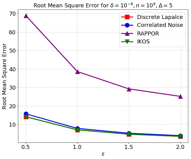
(a) RMSEs for varying $\varepsilon$

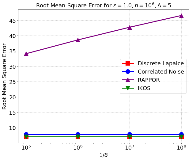
(b) RMSEs for varying $\delta$

Figure 3: Error of our “correlated noise” real-summation protocol compared to other protocols on the rent dataset when varying $\varepsilon$ or $\delta$.

Communication.

The number of bits required for the central DP algorithm remains constant (i.e., $\lceil\log\Delta\rceil$) regardless of the values of $\delta$ or $\varepsilon$. In all other algorithms, the expected number of bits sent per user decreases when $\delta$ or $\varepsilon$ increases. These are demonstrated in Figure 4. We remark that this also holds for RAPPOR, even thought it might be hard to see from the plots because, in our regime of parameters, RAPPOR is within 0.1% of the central DP algorithm.

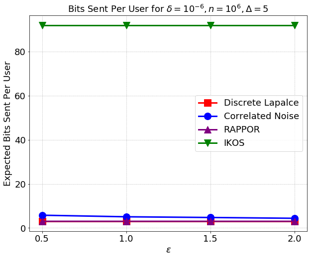
(a) Expected bits sent for varying $\varepsilon$

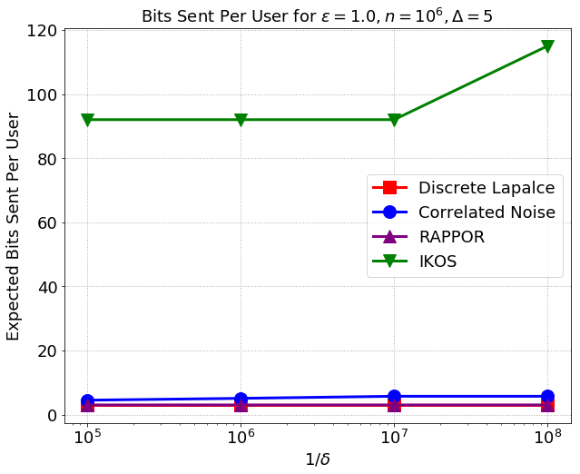
(b) Expected bits sent for varying $\delta$

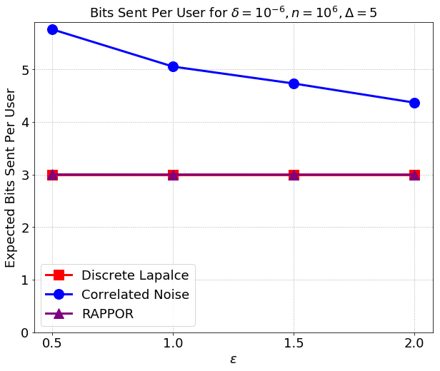
(c) Expected bits sent for varying $\varepsilon$ (without IKOS)

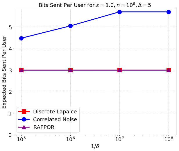
(d) Expected bits sent for varying $\delta$ (without IKOS)

Figure 4: Communication complexity of our “correlated noise” real-summation protocol compared to other protocols on the rent dataset when varying $\varepsilon$ or $\delta$. Since the number of bits sent in the IKOS algorithm is usually very large, it is hard to distinguish the other three lines in the plots where it is included; so we provide the plots without the IKOS algorithm as well.

H.3 Experiments on Real Summation

We evaluate our algorithm on the public $1940$ US Census IPUMS dataset Ruggles et al. (2020). We consider the household rent feature in this dataset; and consider the task of computing the average rent. We restrict to the rents below $\$400$; this reduced the number of reported rents from $68,290,222$ to $66,994,267$, preserving more than $98\%$ of the data. We use randomized rounding (see the proof of Theorem 1) with number of discretization levels $\Delta=20,50,100,200$. Note that 200 is the highest “natural” discretization that is non-trivial in our dataset, since the dataset only contains integers between 0 and 400.

We remark that, for all algorithms, the RMSE is input-dependent but there is still an explicit formula for it; the plots shown below use this formula. On the other hand, the communication bounds do not depend on the input dataset.

Error.

In terms of the errors, unfortunately all of the shuffle DP mechanisms incur significantly higher errors than the Laplace mechanism in central DP. The reason is that the discretization (i.e., randomized rounding) error is already very large, even for the largest discretization level of $\Delta=200$. Nonetheless, the errors for both our algorithm and IKOS decrease as the discretization level increases. Specifically, when $\Delta=200$, the RMSEs for both of these mechanisms are less than half the RMSE of RAPPOR for any number of discretization levels. Notice also that the error for RAPPOR increases for large $\Delta$; the reason is that, as shown in Section 5, the error of RAPPOR grows with $\Delta$ even without discretization. These results are shown in Figure 5(a).

Communication.

In terms of communication, we compare to the non-private “Discretized” algorithm that just discretizes the input into $\Delta$ levels and sends it to the analyzer; it requires only one message of $\lceil\log\Delta\rceil$ bits. RAPPOR incurs little (less than $1\%$) overhead, in expected number of bits sent, compared to this baseline. When $\Delta$ is small, our correlated noise algorithm incurs a small amount of overhead (less than $20\%$ for $\Delta=25$), but this overhead grows moderately as $\Delta$ grows (i.e., to less than $60\%$ for $\Delta=200$). Finally, we note that, since the number $n$ of users is very large, the message length of IKOS (which must be at least $\log n\Delta$) is already large and thus the number of bits sent per user is very large — more than 10 times the baseline.

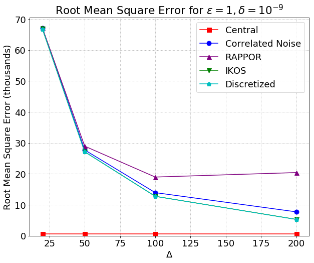
(a) RMSEs for varying $\Delta$

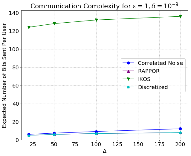
(b) Expected bits sent for varying $\Delta$

Figure 5: Error and communication complexity of our “correlated noise” real-summation protocol compared to other protocols on the rent dataset. The Laplace mechanism is included for comparison in the RMSE plot, even though it is not implementable in the shuffle model; it is not included in the communication plot since the communication is not well-defined. For both plots, we also include “Discretized” which is a non-private algorithm that just discretizes the input and sends it to the analyzer, which then sums up all the incoming messages.

References

- Abadi et al. (2016) Abadi, M., Chu, A., Goodfellow, I., McMahan, H. B., Mironov, I., Talwar, K., and Zhang, L. Deep learning with differential privacy. In CCS, pp. 308–318, 2016.
- Abowd (2018) Abowd, J. M. The US Census Bureau adopts differential privacy. In KDD, pp. 2867–2867, 2018.
- Acharya et al. (2019) Acharya, J., Sun, Z., and Zhang, H. Hadamard response: Estimating distributions privately, efficiently, and with little communication. In AISTATS, pp. 1120–1129, 2019.
- Agarwal et al. (2018) Agarwal, N., Suresh, A. T., Yu, F., Kumar, S., and McMahan, H. B. cpSGD: communication-efficient and differentially-private distributed SGD. In NeurIPS, pp. 7575–7586, 2018.
- Alistarh et al. (2017) Alistarh, D., Grubic, D., Li, J., Tomioka, R., and Vojnovic, M. QSGD: communication-efficient SGD via gradient quantization and encoding. In NIPS, pp. 1709–1720, 2017.
- Apple Differential Privacy Team (2017) Apple Differential Privacy Team. Learning with privacy at scale. Apple Machine Learning Journal, 2017.
- Balcer & Cheu (2020) Balcer, V. and Cheu, A. Separating local & shuffled differential privacy via histograms. In ITC, pp. 1:1–1:14, 2020.
- Balcer et al. (2021) Balcer, V., Cheu, A., Joseph, M., and Mao, J. Connecting robust shuffle privacy and pan-privacy. In SODA, pp. 2384–2403, 2021.
- Balle et al. (2019) Balle, B., Bell, J., Gascón, A., and Nissim, K. The privacy blanket of the shuffle model. In CRYPTO, pp. 638–667, 2019.
- Balle et al. (2020) Balle, B., Bell, J., Gascón, A., and Nissim, K. Private summation in the multi-message shuffle model. In CCS, pp. 657–676, 2020.
- Bassily et al. (2014) Bassily, R., Smith, A., and Thakurta, A. Private empirical risk minimization: Efficient algorithms and tight error bounds. In FOCS, pp. 464–473, 2014.
- Beimel et al. (2008) Beimel, A., Nissim, K., and Omri, E. Distributed private data analysis: Simultaneously solving how and what. In CRYPTO, pp. 451–468, 2008.
- Biswas et al. (2020) Biswas, S., Dong, Y., Kamath, G., and Ullman, J. R. Coinpress: Practical private mean and covariance estimation. In NeurIPS, 2020.
- Bittau et al. (2017) Bittau, A., Erlingsson, Ú., Maniatis, P., Mironov, I., Raghunathan, A., Lie, D., Rudominer, M., Kode, U., Tinnés, J., and Seefeld, B. Prochlo: Strong privacy for analytics in the crowd. In SOSP, pp. 441–459, 2017.
- Chan et al. (2012) Chan, T. H., Shi, E., and Song, D. Optimal lower bound for differentially private multi-party aggregation. In ESA, pp. 277–288, 2012.
- Chang et al. (2021) Chang, A., Ghazi, B., Kumar, R., and Manurangsi, P. Locally private -means in one round. In ICML, 2021.
- Chen et al. (2021) Chen, L., Ghazi, B., Kumar, R., and Manurangsi, P. On distributed differential privacy and counting distinct elements. In ITCS, 2021.
- Chen et al. (2020) Chen, W.-N., Kairouz, P., and Özgür, A. Breaking the communication-privacy-accuracy trilemma. In NeurIPS, 2020.
- Cheu & Zhilyaev (2021) Cheu, A. and Zhilyaev, M. Differentially private histograms in the shuffle model from fake users. CoRR, abs/2104.02739, 2021.
- Cheu et al. (2019) Cheu, A., Smith, A. D., Ullman, J., Zeber, D., and Zhilyaev, M. Distributed differential privacy via shuffling. In EUROCRYPT, pp. 375–403, 2019.
- Ding et al. (2017) Ding, B., Kulkarni, J., and Yekhanin, S. Collecting telemetry data privately. In NIPS, pp. 3571–3580, 2017.
- Dwork et al. (2006a) Dwork, C., Kenthapadi, K., McSherry, F., Mironov, I., and Naor, M. Our data, ourselves: Privacy via distributed noise generation. In EUROCRYPT, pp. 486–503, 2006a.
- Dwork et al. (2006b) Dwork, C., McSherry, F., Nissim, K., and Smith, A. Calibrating noise to sensitivity in private data analysis. In TCC, pp. 265–284, 2006b.
- Erlingsson et al. (2014) Erlingsson, Ú., Pihur, V., and Korolova, A. RAPPOR: Randomized aggregatable privacy-preserving ordinal response. In CCS, pp. 1054–1067, 2014.
- Erlingsson et al. (2019) Erlingsson, Ú., Feldman, V., Mironov, I., Raghunathan, A., Talwar, K., and Thakurta, A. Amplification by shuffling: From local to central differential privacy via anonymity. In SODA, pp. 2468–2479, 2019.
- Erlingsson et al. (2020) Erlingsson, Ú., Feldman, V., Mironov, I., Raghunathan, A., Song, S., Talwar, K., and Thakurta, A. Encode, shuffle, analyze privacy revisited: Formalizations and empirical evaluation. CoRR, abs/2001.03618, 2020.
- Gaboardi et al. (2019) Gaboardi, M., Rogers, R., and Sheffet, O. Locally private mean estimation: -test and tight confidence intervals. In AISTATS, pp. 2545–2554, 2019.
- Geng & Viswanath (2016) Geng, Q. and Viswanath, P. The optimal noise-adding mechanism in differential privacy. IEEE TOIT, 62(2):925–951, 2016.
- Geng et al. (2015) Geng, Q., Kairouz, P., Oh, S., and Viswanath, P. The staircase mechanism in differential privacy. IEEE J. Sel. Top. Signal Process., 9(7):1176–1184, 2015.
- Ghazi et al. (2020a) Ghazi, B., Golowich, N., Kumar, R., Manurangsi, P., Pagh, R., and Velingker, A. Pure differentially private summation from anonymous messages. In ITC, 2020a.
- Ghazi et al. (2020b) Ghazi, B., Kumar, R., Manurangsi, P., and Pagh, R. Private counting from anonymous messages: Near-optimal accuracy with vanishing communication overhead. In ICML, pp. 3505–3514, 2020b.
- Ghazi et al. (2020c) Ghazi, B., Manurangsi, P., Pagh, R., and Velingker, A. Private aggregation from fewer anonymous messages. In EUROCRYPT, pp. 798–827, 2020c.
- Ghazi et al. (2021a) Ghazi, B., Golowich, N., Kumar, R., Pagh, R., and Velingker, A. On the power of multiple anonymous messages. In EUROCRYPT, 2021a.
- Ghazi et al. (2021b) Ghazi, B., Kumar, R., Manurangsi, P., and Pagh, R. Private counting from anonymous messages: Near-optimal accuracy with vanishing communication overhead. CoRR, abs/2106.04247, 2021b. This version contains a correction of calculation errors in Theorem 13 of Ghazi et al. (2020b).
- Ghosh et al. (2012) Ghosh, A., Roughgarden, T., and Sundararajan, M. Universally utility-maximizing privacy mechanisms. SIAM J. Comput., 41(6):1673–1693, 2012.
- Girgis et al. (2021) Girgis, A. M., Data, D., Diggavi, S., Kairouz, P., and Suresh, A. T. Shuffled model of federated learning: Privacy, communication and accuracy trade-offs. In AISTATS, 2021.
- Goryczka & Xiong (2017) Goryczka, S. and Xiong, L. A comprehensive comparison of multiparty secure additions with differential privacy. IEEE Trans. Dependable Secur. Comput., 14(5):463–477, 2017.
- Greenberg (2016) Greenberg, A. Apple’s “differential privacy” is about collecting your data – but not your data. Wired, June, 13, 2016.
- Ishai et al. (2006) Ishai, Y., Kushilevitz, E., Ostrovsky, R., and Sahai, A. Cryptography from anonymity. In FOCS, pp. 239–248, 2006.
- Kairouz et al. (2019) Kairouz, P., McMahan, H. B., Avent, B., Bellet, A., Bennis, M., Bhagoji, A. N., Bonawitz, K., Charles, Z., Cormode, G., Cummings, R., et al. Advances and open problems in federated learning. CoRR, abs/1912.04977, 2019.
- Kasiviswanathan et al. (2008) Kasiviswanathan, S. P., Lee, H. K., Nissim, K., Rashkodnikova, S., and Smith, A. What can we learn privately? In FOCS, pp. 531–540, 2008.
- Nikolov et al. (2013) Nikolov, A., Talwar, K., and Zhang, L. The geometry of differential privacy: the sparse and approximate cases. In STOC, pp. 351–360, 2013. doi: 10.1145/2488608.2488652. URL https://doi.org/10.1145/2488608.2488652.
- Ruggles et al. (2020) Ruggles, S., Flood, S., Goeken, R., Grover, J., Meyer, E., Pacas, J., and Sobek, M. Integrated public use microdata series (IPUMS) USA: Version 10.0 [dataset]. Minneapolis, MN, 2020. URL https://doi.org/10.18128/D010.V10.0.
- Shankland (2014) Shankland, S. How Google tricks itself to protect Chrome user privacy. CNET, October, 2014.
- Song et al. (2013) Song, S., Chaudhuri, K., and Sarwate, A. D. Stochastic gradient descent with differentially private updates. In GlobalSIP, pp. 245–248, 2013.
- Stemmer (2020) Stemmer, U. Locally private k-means clustering. In SODA, pp. 548–559, 2020.
- Stemmer & Kaplan (2018) Stemmer, U. and Kaplan, H. Differentially private -means with constant multiplicative error. In NeurIPS, pp. 5436–5446, 2018.
- Suresh et al. (2017) Suresh, A. T., Felix, X. Y., Kumar, S., and McMahan, H. B. Distributed mean estimation with limited communication. In ICML, pp. 3329–3337, 2017.
- Warner (1965) Warner, S. L. Randomized response: A survey technique for eliminating evasive answer bias. JASA, 60(309):63–69, 1965.
- Zhang et al. (2013) Zhang, Y., Duchi, J. C., Jordan, M. I., and Wainwright, M. J. Information-theoretic lower bounds for distributed statistical estimation with communication constraints. In NIPS, pp. 2328–2336, 2013.