The motion of an unbalanced circular foil in the field of a point source

¹Ural Mathematical Center, Udmurt State University, Universitetskaya 1, Izhevsk, 426034 Russia

²Kalashnikov Izhevsk State Technical University, Studencheskaya 7, Izhevsk 426069, Russia

^∗liz-artemova2014@yandex.ru ⁺eugene186@mail.ru

Abstract.

Describing the phenomena of the surrounding world is an interesting task that has long attracted the attention of scientists. However, even in seemingly simple phenomena, complex dynamics can be revealed. In particular, leaves on the surface of various bodies of water exhibit complex behavior. This paper addresses an idealized description of the mentioned phenomenon. Namely, the problem of the plane-parallel motion of an unbalanced circular disk moving in a stream of simple structure created by a point source is considered. Note that using point sources, it is possible to approximately simulate the work of skimmers used for cleaning swimming pools. Equations of joint motion of the unbalanced circular disk and the point source. It is shown that in the case of a fixed source of constant intensity the equations of motion of the disk are Hamiltonian. In addition, in the case of a balanced circular disk the equations of motion are integrable. A bifurcation analysis of the integrable case is carried out. Using a scattering map, it is shown that the equations of motion of the unbalanced disk are nonintegrable. The nonintegrability found here can explain the complex motion of leaves in surface streams of bodies of water.

1 Introduction

The study of the motion of point singularities constitutes a fairly large part of theoretical hydrodynamics. In this field, one of the classical problems going back to the works of Helmholtz [1] and Kirchhoff [2] is that of the motion of rectilinear parallel vortex filaments in an ideal fluid, which is also called the problem of the motion of $N$ point vortices on a plane. It should be noted that the equations of motion are integrable for $N\leq 3$, and in the case $N\geq 4$ this system is nonintegrable and can exhibit chaotic behavior [3, 4].

The conception of a point vortex was applied in various problem statements. For example, this model was used to address the problem of the stability of polygonal vortex configurations on a plane [5], on a sphere [6], in spaces of constant curvature [7], and in a circle [8]. A wide review of research results on vortex dynamics is presented in the monograph [9]. The problem of the perturbation of the motion of two point vortices by an acoustic wave is dealt with in [10]. A similar problem with addition of background shear flow is treated in [11].

Equations similar to the equations of motion of point vortices arise in the description of the motion of point singularities in a Bose – Einstein condensate [12, 13, 14] and hetons [15, 16], oceanic vortex structures existing in a stratified fluid. The description of the motion of vortex rings also involves equations similar to the equations of motion of point vortices [17, 18, 19, 20].

The point vortex model is also brought to bear to derive finite-dimensional equations describing the joint motion of vortex structures and a rigid body. The equations of motion of a balanced circular foil in the presence of point vortices were obtained for the first time in [21, 22, 23]. The motion of an unbalanced circular foil in the presence of point vortices has recently been examined in [24]. We note that the displacement of the center of mass of the circular foil leads to the loss of additional symmetry and gives rise to obstructions to integrability. In particular, the problem of the motion of a balanced circular foil and a point vortex is integrable, and in the case of a circular foil with a displaced center of mass the system becomes nonintegrable and can exhibit chaotic behavior.

We note that the model of a point vortex can be used for a phenomenological description of the shedding of vortices from a sharp edge of a rigid body performing unsteady motion [25, 26, 27].

In addition to point vortices, one considers (fairly rarely) the motion of other point singularities in a fluid, such as sources, vortex sources, and dipoles [28, 29, 30, 31]. In our recent paper [32], we proposed a finite-dimensional model describing the motion of a balanced circular foil in the field of a fixed source. It was shown that the system is integrable and admits one unstable periodic solution. It was shown that this solution can be stabilized by changing the intensity of the source via feedback.

In this paper we develop the study presented in [32], and consider the motion of an unbalanced circular foil in the field of a point source. We derive equations of joint motion of motion of a source whose intensity depends on time and of an unbalanced circular foil. We show that, in the case of a fixed source of constant intensity, the equations of motion of the circular foil are Hamiltonian. We perform a bifurcation analysis of the dynamics for the case of a balanced foil. In the system under consideration we have found no stable compact trajectories, and therefore we carry out its numerical investigation using a scattering map instead of the traditional Poincaré map. Using such a map, we show that, in the case of an unbalanced foil, the equations of motion are nonintegrable.

The model presented in this paper can be considered as an idealized description of the motion of leaves in streams on the surface of water bodies. Unconditionally, natural flows have a complex structure that is significantly different from the structure of the flow created by a point source. Nevertheless, even in the case of the considered simple flow, the derived equations of motion turn out to be nonintegrable. The nonintegrability found here can be used as an explanation of the complex motion of leaves in streams observed in nature.

2 A mathematical model

2.1 The case of a moving source of variable intensity

Consider the plane-parallel motion of an unbalanced circular foil in the presence of a point source in an unbounded volume of an ideal incompressible fluid. We assume that the fluid performs potential noncircular motion and is at rest at infinity.

To construct a mathematical model, we introduce the following notation for the system parameters:

• $m_{c}$ is the mass of the foil,

• $I_{c}$ is the central moment of inertia of the foil,

• $R$ is the radius of the foil,

• $d$ is the distance between the geometric center of the foil and the center of mass,

• $q$ is the intensity of the source, which is generally a given function of time.

Since we consider the plane-parallel motion, we will assume the parameters $m_{c}$, $I_{c}$ and $q$ to be related to the unit of length of the foil.

To describe the motion of the system, we introduce three coordinate systems: a fixed (inertial) system $OXY$, a moving system $Cx^{\prime}y^{\prime}$, rigidly attached to the foil, and a coordinate system $Oxy$ rotating synchronously with the foil (see Fig. 1). We will assume that the origin of the moving coordinate system $C$ is at the geometric center of the foil and that the center of mass of the foil lies on the positive part of the axis $Cx^{\prime}$.

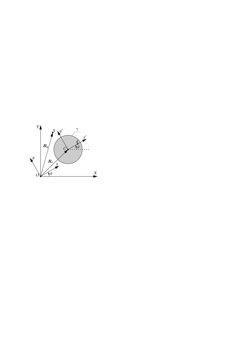
Figure 1: A schematic diagram of an unbalanced circular foil and a point source.

We will specify the position of the foil relative to the fixed coordinate system by the radius vector of its geometric center $\boldsymbol{R}_{c}=(X_{c},\,Y_{c})$, and the orientation of the foil, by the angle $\vartheta$ between the positive directions of the axes $OX$ and $Cx^{\prime}$. The position of the source relative to the fixed coordinate system will be specified by the radius vector $\boldsymbol{R}_{q}=(X_{q},\,Y_{q})$. Thus, the configuration space of the system is five-dimensional and is $\mathcal{Q}=\bigl{\{}\left(X_{q},\,Y_{q},\,X_{c},\,Y_{c},\,\vartheta\right)\ |\ (X_{q}-X_{c})^{2}+(Y_{q}-Y_{c})^{2}>R^{2}\bigr{\}}\approx\mathbb{R}^{3}\times\mathbb{T}^{2}$. The quantities defining the configuration of the system are shown in Fig. 1.

The motion of the system is determined by the interaction of the foil and the source with the surrounding fluid. Since the motion of the fluid is assumed to be potential, it can be completely described by a complex potential. To construct the complex potential, to each point of the plane $OXY$ we associate the complex number $Z=X+iY$. Then the complex potential can be written as

$$W=-\frac{R^{2}\dot{Z}_{c}}{Z-Z_{c}}+\frac{q}{2\pi}\ln(Z-Z_{q})+\frac{q}{2\pi}\ln\biggl{(}\frac{R^{2}}{Z-Z_{c}}-\overline{Z_{q}-Z_{c}}\biggr{)},$$ (1)

where $Z_{c}=X_{c}+iY_{c}$, $Z_{q}=X_{q}+iY_{q}$ are complex-valued functions of time which define the position of the center of the foil and the source, respectively.

Remark 1.

The first and second terms in the expression (1) are complex potentials of the moving cylinder and the source, respectively [33]. The third term in the expression (1) arises by applying the Milne – Thomson theorem [34] and describes the change of the flow created by the source, which occurs due to a circular foil being added to it.

To construct the equations of motion, we introduce the following quantities:

$$\begin{gathered}P_{x}=m_{c}\dot{X}_{c}-m_{c}d\dot{\vartheta}\sin\vartheta,\quad P_{y}=m_{c}\dot{Y}_{c}+m_{c}d\dot{\vartheta}\cos\vartheta,\\ P_{\vartheta}=m_{c}d(-\dot{X}_{c}\sin\vartheta+\dot{Y}_{c}\cos\vartheta)+(I_{c}+m_{c}d^{2})\dot{\vartheta},\end{gathered}$$ (4)

where $P_{x}$ and $P_{y}$ are the projections of the momentum of the foil onto the axes of the fixed coordinate system and $P_{\vartheta}$ is the angular momentum of the foil relative to its geometric center.

The change in the momentum of the foil is defined by the principal vector of pressure forces $\boldsymbol{F}=(F_{x},\,F_{y})$ acting on it from the fluid. The components of the vector $\boldsymbol{F}$ can be calculated from Sedov’s formula [35]:

$$F_{x}+iF_{y}=\overline{\frac{i\rho}{2}\oint\limits_{\gamma}\bigg{(}\frac{dW}{dZ}\bigg{)}^{2}dZ}+\frac{d}{dt}\bigg{(}\rho\frac{dSZ_{c}}{dt}+i\rho\oint\limits_{\gamma}Z\frac{dW}{dZ}dZ\bigg{)}.$$ (5)

Here $\rho$ is the density of the fluid, $S=\pi R^{2}$ is the area of the foil, and $\gamma$ is the boundary of the circular foil. Since the motion of the fluid is assumed to be noncircular, the terms related to circulation are omitted in the formula (5).

Substituting the potential (1) into the formula (5), we obtain an explicit expression for the components of the principal pressure force vector:

$$F_{x}+iF_{y}=\rho qR^{2}\frac{(Z_{q}-Z_{c})^{2}}{|Z_{q}-Z_{c}|^{4}}\dot{\overline{Z_{q}}}-\rho\dot{q}R^{2}\frac{Z_{q}-Z_{c}}{|Z_{q}-Z_{c}|^{2}}+\\ +\frac{\rho q^{2}R^{2}}{2\pi}\frac{(Z_{q}-Z_{c})}{(|Z_{q}-Z_{c}|^{2}-R^{2})|Z_{q}-Z_{c}|^{2}}-\rho\pi R^{2}\ddot{Z}_{c}.$$ (6)

The components $F_{x}$ and $F_{y}$ thus calculated are related to the unit of length of the cylinder. The last term in the expression (6) coincides with the classical expression for the force due to the effect of added masses [36] and acting on the circular foil when it performs accelerated motion.

Remark 2.

We note that the calculation of the forces (6) can also be performed in the real form

$$F_{x}=-\oint\limits_{\gamma}pdy,\quad F_{x}=\oint\limits_{\gamma}pdx,$$

where the pressure $p$ is unambiguously calculated using the Cauchy – Lagrange integral [33]. However, calculations in complex form with the aid of the formula (5) are simpler in practice.

Since the foil is circular, the pressure torque calculated relative to the geometric center of the foil is zero. In this case, the angular momentum $P_{\vartheta}$ can change only due to the rotation of the foil. Thus, the equations of motion of the foil take the form

$$\dot{P}_{x}=F_{x},\quad\dot{P}_{y}=F_{y},\quad\dot{P}_{\vartheta}+d(P_{x}\cos\vartheta+P_{y}\sin\vartheta)\dot{\vartheta}=0.$$ (7)

We supplement equations (7) with the equations of motion of the source. According to [28], the velocity of the motion of the source is equal to the velocity of the fluid at the point $Z=Z_{q}$ calculated from the regular part of the potential (1) at the same point:

$$\dot{Z}_{q}=\overline{\left(\frac{dW^{*}}{dZ}\right)}\bigg{|}_{Z=Z_{q}},\quad W^{*}=W-\frac{q}{2\pi}\ln(Z-Z_{q}).$$ (8)

Equations (4), (7) and (8) are a closed system and completely describe the joint motion of the circular foil and the point source of variable intensity in an ideal fluid.

2.2 The case of a moving source of constant intensity

In the case of a source of constant intensity ($\dot{q}=0$) the equations of motion of the foil (7) can be represented in the Lagrangian form

$$\frac{d}{dt}\frac{\partial L}{\partial\dot{X}_{c}}-\frac{\partial L}{\partial X_{c}}=0,\quad\frac{d}{dt}\frac{\partial L}{\partial\dot{Y}_{c}}-\frac{\partial L}{\partial Y_{c}}=0,\quad\frac{d}{dt}\frac{\partial L}{\partial\dot{\vartheta}}-\frac{\partial L}{\partial\vartheta}=0$$ (9)

with the Lagrangian

$$L=T-U-\left(\boldsymbol{A},\,\dot{\boldsymbol{R}}_{c}\right),$$ (10)

where the following notation has been introduced:

1. $T$ is the kinetic energy of the foil and the fluid

   $$T=\frac{1}{2}\left(m_{c}+\rho\pi R^{2}\right)\left(\dot{X}_{c}^{2}+\dot{Y}_{c}^{2}\right)+m_{c}d\left(-\sin\vartheta\dot{X}_{c}+\cos\vartheta\dot{Y}_{c}\right)\dot{\vartheta}+\frac{1}{2}\left(I_{c}+m_{c}d^{2}\right)\dot{\vartheta}^{2},$$

2. $U$ is the scalar potential

   $$U=-\frac{\rho q^{2}}{4\pi}\Bigl{(}\ln\bigl{(}(X_{c}-X_{q})^{2}+(Y_{c}-Y_{q})^{2}\bigr{)}-\ln\bigl{(}(X_{c}-X_{q})^{2}+(Y_{c}-Y_{q})^{2}-R^{2}\bigr{)}\Bigr{)},$$

3. $\boldsymbol{A}$ is the vector potential

   $$\boldsymbol{A}=-\frac{\rho qR^{2}}{(X_{q}-X_{c})^{2}+(Y_{q}-Y_{c})^{2}}\left(\boldsymbol{R}_{q}-\boldsymbol{R}_{c}\right).$$

The right-hand sides of the equations of motion of the source (8) are also expressed in terms of the Lagrangian (10) as follows:

$$\dot{X}_{q}=-\frac{1}{\rho q}\frac{\partial L}{\partial X_{q}},\quad\dot{Y}_{q}=-\frac{1}{\rho q}\frac{\partial L}{\partial Y_{q}}.$$ (11)

Thus, we have obtained a system of equations (9) and (11) in a partially Lagrangian form which describes the joint motion of the circular foil and the source of constant intensity.

2.3 The case of a fixed source of constant intensity

In the case of a fixed source of constant intensity ($\dot{X}_{q}=0$, $\dot{Y}_{q}=0$, $\dot{q}=0$) the equations of motion of the foil (9) can be represented in Hamiltonian form. In this case, we will assume without loss of generality that the source lies at the origin of the fixed coordinate system ($X_{q}=Y_{q}=0$). These conditions can always be enforced by making the change of variables

$$X_{c}\to X_{c}-X_{q},\quad Y_{c}\to Y_{c}-Y_{q}.$$

To reduce equations (9) to Hamiltonian form, we introduce new generalized momenta $\Pi_{x}$, $\Pi_{y}$ and $\Pi_{\vartheta}$ as follows:

$$\Pi_{x}=\frac{\partial L}{\partial\dot{X}_{c}}=P_{x}+\rho\pi R^{2}\dot{X}_{c}-A_{x},\quad\Pi_{y}=\frac{\partial L}{\partial\dot{Y}_{c}}=P_{y}+\rho\pi R^{2}\dot{Y}_{c}-A_{y},\quad\Pi_{\vartheta}=\frac{\partial L}{\partial\dot{\vartheta}}=P_{\vartheta},$$ (12)

$$A_{x}=\frac{\rho qR^{2}X_{c}}{X_{c}^{2}+Y_{c}^{2}},\quad A_{y}=\frac{\rho qR^{2}Y_{c}}{X_{c}^{2}+Y_{c}^{2}}$$

and perform the Legendre transformation

$$H=\Pi_{x}\dot{X}_{c}+\Pi_{y}\dot{Y}_{c}+\Pi_{\vartheta}\dot{\vartheta}-L\Big{|}_{\dot{X}_{c},\,\dot{Y}_{c},\,\dot{\vartheta}\to\Pi_{x},\,\Pi_{y},\,\Pi_{\vartheta}}.$$ (13)

Then the equations of motion of the circular foil (9) take the form

$$\begin{gathered}\dot{X}_{c}=\frac{\partial H}{\partial\Pi_{x}},\quad\dot{Y}_{c}=\frac{\partial H}{\partial\Pi_{y}},\quad\dot{\vartheta}=\frac{\partial H}{\partial\Pi_{\vartheta}}\\ \dot{\Pi}_{x}=-\frac{\partial H}{\partial X_{c}},\quad\dot{\Pi}_{y}=-\frac{\partial H}{\partial Y_{c}},\quad\dot{\Pi}_{\vartheta}=-\frac{\partial H}{\partial\vartheta},\end{gathered}$$ (16)

where the Hamiltonian $H$ is given by the following expression:

$$H=\frac{1}{2}\big{(}\boldsymbol{\mathcal{P}},\mathbb{Q}^{-1}\boldsymbol{\mathcal{P}}\big{)}-\frac{\rho q^{2}}{4\pi}\Bigl{(}\ln\bigl{(}X_{c}^{2}+Y_{c}^{2}\bigr{)}-\ln\bigl{(}X_{c}^{2}+Y_{c}^{2}-R^{2}\bigr{)}\Bigr{)},$$ (17)

$$\boldsymbol{\mathcal{P}}=\begin{pmatrix}\Pi_{x}+A_{x}\\ \Pi_{y}+A_{y}\\ \Pi_{\vartheta}\end{pmatrix},\quad\mathbb{Q}=\begin{pmatrix}m_{c}+\rho\pi R^{2}&0&-m_{c}d\sin\vartheta\\ 0&m_{c}+\rho\pi R^{2}&m_{c}d\cos\vartheta\\ -m_{c}d\sin\vartheta&m_{c}d\cos\vartheta&I_{c}+m_{c}d^{2}\end{pmatrix}.$$

Remark 3.

It has not been possible for us to represent in Hamiltonian form the complete system of equations (9) and (11), which describes the joint motion of the circular foil and the point source of constant intensity. The form of the Lagrangian (10) and the form of equations (11) are obstructions to such a representation.

We note that, in a similar system governing the motion of the circular foil in the presence of point vortices [37], representation in Hamiltonian form does turn out to be possible.

Equations (16) admit two first integrals: an energy integral coinciding with the Hamiltonian (17) and the integral of the angular momentum

$$K=\Pi_{\vartheta}+\Pi_{y}X_{c}-\Pi_{x}Y_{c}=\mathrm{const}\,,$$ (18)

which is a consequence of the existence of a symmetry field

$$\boldsymbol{u}=-Y_{c}\frac{\partial}{\partial X_{c}}+X_{c}\frac{\partial}{\partial Y_{c}}+\frac{\partial}{\partial\vartheta}-\Pi_{y}\frac{\partial}{\partial\Pi_{x}}+\Pi_{x}\frac{\partial}{\partial\Pi_{y}}.$$ (19)

We next investigate the dynamics of the system and the properties of equations (16) in the following two cases:

• the case of a balanced foil ($d=0$);

• the case of an unbalanced foil ($d\neq 0$).

3 A balanced cylinder

Consider the motion of a balanced ($d=0$) circular foil in the field of a fixed source of constant intensity. It turns out that in this case a complete qualitative dynamics analysis can be carried out.

If $d=0$, the Hamiltonian (17) takes the form

$$H=H_{rot}+H_{trans},$$ (20)

$$H_{rot}=\frac{1}{2}\frac{\mathcal{P}_{\vartheta}^{2}}{I_{c}},$$ (21)

$$H_{trans}=\frac{1}{2}\left(\frac{\mathcal{P}_{x}^{2}}{m}+\frac{\mathcal{P}_{y}^{2}}{m}\right)-\frac{\rho q^{2}}{4\pi}\Bigl{(}\ln\bigl{(}X_{c}^{2}+Y_{c}^{2}\bigr{)}-\ln\bigl{(}X_{c}^{2}+Y_{c}^{2}-R^{2}\bigr{)}\Bigr{)},$$ (22)

where the following notation has been introduced:

$$\mathcal{P}_{x}=m\dot{X}_{c},\quad\mathcal{P}_{y}=m\dot{Y}_{c},\quad\mathcal{P}_{\vartheta}=m\dot{\vartheta},\quad m=m_{c}+\rho\pi R^{2}.$$ (23)

In this case, equations (16) decouple into two independent subsystems governing the rotational motion

$$\begin{gathered}\quad\dot{\vartheta}=\frac{\partial H}{\partial\mathcal{P}_{\vartheta}}=\frac{\partial H_{rot}}{\partial\mathcal{P}_{\vartheta}},\quad\dot{\mathcal{P}}_{\vartheta}=-\frac{\partial H}{\partial\vartheta}=-\frac{\partial H_{rot}}{\partial\vartheta}\end{gathered}$$ (25)

and the translational motion of the foil

$$\begin{gathered}\dot{X}_{c}=\frac{\partial H}{\partial\mathcal{P}_{x}}=\frac{\partial H_{trans}}{\partial\mathcal{P}_{x}},\quad\dot{\mathcal{P}}_{x}=-\frac{\partial H}{\partial X_{c}}=-\frac{\partial H_{trans}}{\partial X_{c}}\\ \dot{Y}_{c}=\frac{\partial H}{\partial\mathcal{P}_{y}}=\frac{\partial H_{trans}}{\partial\mathcal{P}_{y}},\quad\dot{\mathcal{P}}_{y}=-\frac{\partial H}{\partial Y_{c}}=-\frac{\partial H_{trans}}{\partial Y_{c}}\end{gathered}$$ (28)

with the Hamiltonians (21) and (22), respectively.

We first consider the subsystem (25). Since the Hamiltonian (21) does not explicitly depend on $\vartheta$, this variable is cyclic and the corresponding generalized momentum is a first integral:

$$C=\mathcal{P}_{\vartheta}=\mathrm{const}\,.$$ (29)

On the fixed level set $C=c$ of the first integral (29), the solution of the subsystem (25) can be represented as

$$\mathcal{P}_{\vartheta}=c=\mathrm{const}\,,\quad\vartheta(t)=\vartheta(0)+\frac{c}{I_{c}}t.$$ (30)

Next, we consider the subsystem (28), which can be investigated more conveniently by transforming to the polar coordinates:

$$X_{c}=s\cos\alpha,\quad Y_{c}=s\sin\alpha.$$ (31)

In this case, we define the generalized momenta, which correspond to the coordinates $s$ and $\alpha$, as follows:

$$\mathcal{P}_{s}=m\dot{s},\quad\mathcal{P}_{\alpha}=ms^{2}\dot{\alpha}.$$ (32)

The equations of motion (28) in the new variables (31) and (32) remain canonical:

$$\dot{s}=\frac{\partial H_{trans}}{\partial\mathcal{P}_{s}},\quad\dot{\alpha}=\frac{\partial H_{trans}}{\partial\mathcal{P}_{\alpha}},\quad\dot{\mathcal{P}}_{s}=-\frac{\partial H_{trans}}{\partial s},\quad\dot{\mathcal{P}}_{\alpha}=-\frac{\partial H_{trans}}{\partial\alpha},$$ (33)

where the Hamiltonian (22) takes the form

$$H_{trans}=\frac{1}{2m}\left(\mathcal{P}_{s}^{2}+\frac{\mathcal{P}_{\alpha}^{2}}{s^{2}}\right)+\frac{\rho q^{2}}{4\pi}\ln\biggl{(}1-\frac{R^{2}}{s^{2}}\biggr{)}.$$ (34)

The Hamiltonian (34) does not explicitly depend on the angle $\alpha$. Hence, the generalized momentum $\mathcal{P}_{\alpha}$ is a first integral:

$$F=\mathcal{P}_{\alpha}=\mathrm{const}\,.$$ (35)

Remark 4.

In the case considered here ($d=0$), using the expressions (31) and (32), the first integral (18) can be represented as

$$K=\mathcal{P}_{\vartheta}+\mathcal{P}_{\alpha}=C+F=\mathrm{const}\,.$$

On the fixed level set $F=f$ of the first integral (35) the equations for $s$ and $\mathcal{P}_{s}$ decouple from the system (33) and take the form

$$\dot{s}=\frac{\mathcal{P}_{s}}{m},\quad\dot{\mathcal{P}}_{s}=\frac{f^{2}}{ms^{3}}-\frac{\rho q^{2}R^{2}}{2\pi s(s^{2}-R^{2})}.$$ (36)

In this case, the evolution of the phase variable $\alpha$ is expressed by the quadrature

$$\alpha(t)=\alpha(0)+\frac{f}{m}\int\limits_{0}^{t}\frac{d\tau}{s^{2}(\tau)}.$$

This quadrature is necessary for reconstruction of the foil’s motion relative to the fixed coordinate system.

Equations (36) admit the first integral

$$H_{trans}=\frac{1}{2m}\mathcal{P}_{s}^{2}+U(s),$$ (37)

$$U(s)=\frac{1}{2m}\frac{f^{2}}{s^{2}}+\frac{\rho q^{2}}{4\pi}\ln\biggl{(}1-\frac{R^{2}}{s^{2}}\biggr{)},$$ (38)

which is a restriction of the Hamiltonian (34) to the fixed level set $F=f$ of the integral (35). Also, equations (36) have the involution

$$t\to-t,\quad s\to s,\quad\mathcal{P}_{s}\to-\mathcal{P}_{s}.$$ (39)

Remark 5.

The motions of the reduced system (36) with $F=f>0$ are identical with those with $F=-f$. Consequently, it suffices to analyze the dynamics for $f>0$.

Equations (36) are a Hamiltonian system with one degree of freedom. In our analysis of this system we will use the classical approach of theoretical mechanics which is based on the study of the level lines of the Hamiltonian (phase portrait) of the system and bifurcations arising as the parameter values are varied [38, 39].

We first note that the Hamiltonian (37) is defined for $s>R$ and, regardless of the parameter values, possesses the following property:

$$\lim\limits_{s\to R+0}H_{trans}(s,\mathcal{P}_{s})=-\infty.$$ (40)

Also, the Hamiltonian (37) is an even function of $\mathcal{P}_{s}$, i.e., $H_{trans}(s,-\mathcal{P}_{s})=H_{trans}(s,\mathcal{P}_{s})$, and hence the phase portrait of the system will be symmetric relative to the line $\mathcal{P}_{s}=0$. It is seen from equations (36) that the fixed points of the system can lie only on the line $\mathcal{P}_{s}=0$ and that they correspond to the critical points of the potential (38).

Two qualitatively different cases can be singled out:

• The potential $U(s)$ (see Fig. 2b) has a maximum at the point

  $$s_{0}=R|f|\sqrt{\frac{2\pi}{2\pi f^{2}-\rho mq^{2}R^{2}}}$$ (41)

  for $f>f_{cr}$, where

  $$f_{cr}=|q|R\sqrt{\frac{\rho m}{2\pi}}.$$

  The maximum point (41) corresponds to the fixed saddle point of the system (36):

  $$s=s_{0},\quad\mathcal{P}_{s}=0.$$ (42)

  A typical view of the phase portrait of the system for $f>f_{cr}$ is shown in Fig. 2d. The red dashed lines in Fig. 2d indicate stable and unstable manifolds of the saddle point (42). The dashed line $s=R$ corresponds to the singularity (40).

• If $f<f_{cr}$, the potential $U(s)$ is a monotonically increasing function on the interval $s\in(R,+\infty)$ (see Fig. 2a). Hence, the system has no fixed points. A typical view of the phase portrait of the system for $f<f_{cr}$ is shown in Fig. 2c. The red dashed lines in Fig. 2c denote the critical trajectories separating different types of motion. The dashed line $s=R$ corresponds to the singularity (40).

It can be seen from the phase portraits (see Fig. 2c and 2d) that all trajectories of the system (36) either go to infinity or “fall” on a source, except for one trajectory corresponding to a fixed point when $f>f_{cr}$.

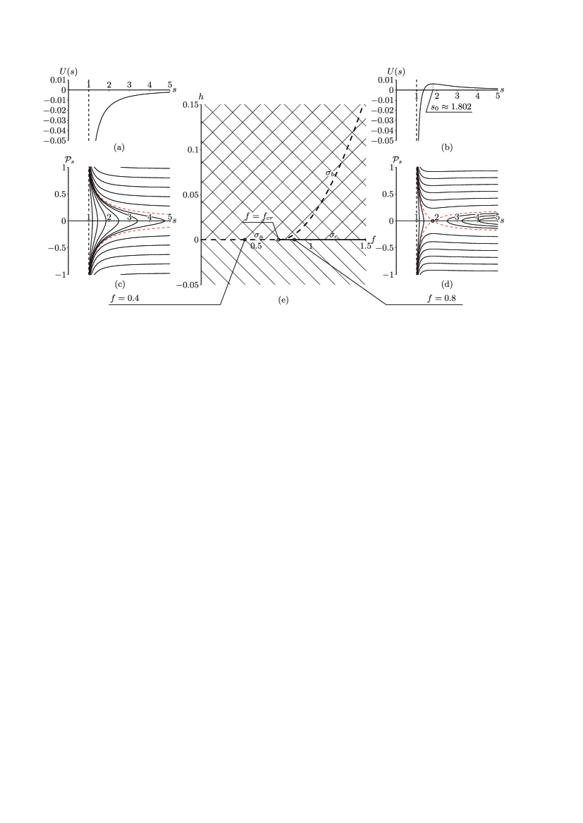
Figure 2: A typical view of a) the potential (38) for $f<f_{cr}$, b) the potential (38) for $f>f_{cr}$, c) the phase portrait of the system for $f<f_{cr}$, and d) the phase portrait of the system for $f>f_{cr}$. e) Bifurcation diagram. The parameter values: $m_{c}=1$, $R=1$, $q=1$, $\rho=1$.

A bifurcation diagram of the system on the plane of first integrals $(f,\,h)$, where $h$ is a level set of the integral (37), is shown in Fig. 2e. In view of Remark 5 we have presented only a part of the bifurcation diagram which corresponds to the values $f>0$.

If $f$ is fixed, to each value of $h>0$ (the double hatched area in Fig. 2e) there correspond two phase trajectories, and to the value of $h<0$ (the single hatched area in Fig. 2e), one phase trajectory. The bifurcation diagram 2e corresponds to the bifurcation complex shown in Fig. 3.

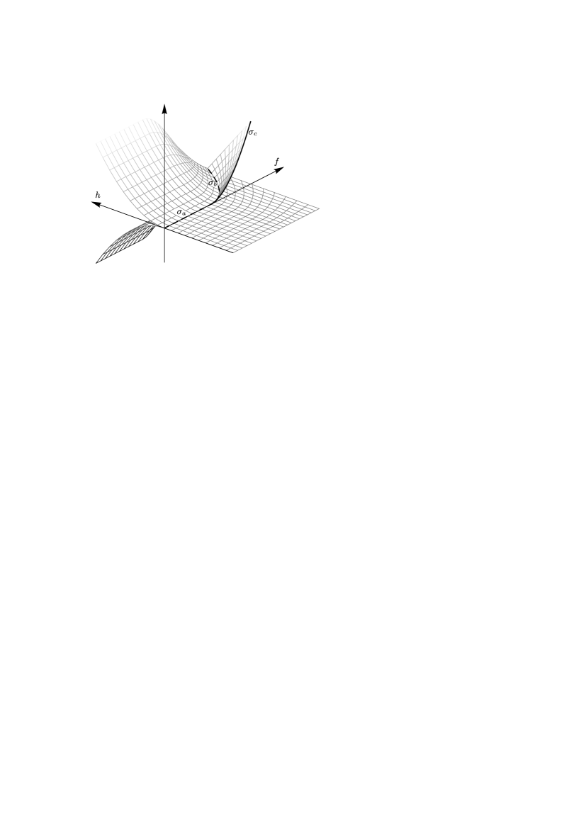
Figure 3: Bifurcation complex. The vertical axis in this picture has no physical meaning and is used merely for convenience of visualization of different leaves

The line $\sigma_{a}$ corresponds to critical trajectories of the system which arise in the system for $f<f_{cr}$. The line $\sigma_{b}$ corresponds to the fixed point (42) and to its stable and unstable manifolds. The line $\sigma_{c}$ corresponds to the boundary of the leaf.

Remark 6.

We note that the fixed point (42) of the reduced system (36) can be stabilized via feedback [32]. In this case, the equations of motion cease to be Hamiltonian.

4 An unbalanced cylinder

We now turn to an analysis of the motion of an unbalanced ($d>0$) circular foil in the field of a fixed source of constant intensity. It turns out that, as in the previous case ($d=0$), examination of the system (16) in the case $d>0$ by analytical methods reveals only a finite number of compact trajectories. Numerical experiments show that the other trajectories of the system are noncompact, i.e., they either go to infinity or “fall” on the source. In addition, when $d>0$, the equations of motion (16) become nonintegrable.

4.1 The hypothesis of noncompactness of phase trajectories

To show the noncompactness of the phase trajectories of the system considered, we single out the effective potential from the Hamiltonian (17). To do so, we make the change of variables

$$x=X_{c}\cos\vartheta+Y_{c}\sin\vartheta,\quad y=-X_{c}\sin\vartheta+Y_{c}\cos\vartheta$$ (43)

and express the Hamiltonian (17) in terms of the derivatives of the coordinates $x$, $y$ and the angle $\vartheta$:

$$\mathcal{H}=\frac{1}{2}\left(\boldsymbol{v},\,\widetilde{\mathbb{Q}}\boldsymbol{v}\right)+\frac{\rho q^{2}}{4\pi}\ln\left(1-\frac{R^{2}}{x^{2}+y^{2}}\right),$$ (44)

$$\widetilde{\mathbb{Q}}=\begin{pmatrix}m&0&0\\ 0&m&m_{c}d\\ 0&m_{c}d&I_{c}+m_{c}d^{2}\end{pmatrix},\quad\boldsymbol{v}=\begin{pmatrix}\dot{x}-y\dot{\vartheta}\\ \dot{y}+x\dot{\vartheta}\\ \dot{\vartheta}\end{pmatrix}.$$

The change of variables (43) enables us to transform to the coordinate system $Oxy$, which rotates synchronously with the foil, and to eliminate the angle variable $\vartheta$ from the Hamiltonian.

We fix the level set $K=k$ of the first integral (18) and express from it the derivative $\dot{\vartheta}$:

$$\dot{\vartheta}=\frac{k+my\dot{x}-(mx+m_{c}d)\dot{y}}{m(x^{2}+y^{2})+2m_{c}dx+I_{c}+m_{c}d^{2}}.$$ (45)

Substituting the expression (45) into the total energy (44), we can write the following representation:

$$\mathcal{H}=\frac{1}{2}\left(\boldsymbol{w},\,\mathbb{R}(x,\,y)\boldsymbol{w}\right)+U_{e}(x,\,y),$$ (46)

$$U_{e}(x,\,y)=\frac{k^{2}}{2\left(m(x^{2}+y^{2})+2m_{c}dx+I_{c}+m_{c}d^{2}\right)}+\frac{\rho q^{2}}{4\pi}\ln\left(1-\frac{R^{2}}{x^{2}+y^{2}}\right),$$ (47)

where $\boldsymbol{w}=(\dot{x},\,\dot{y})^{T}$, $\mathbb{R}(x,\,y)$ is a symmetric positive definite matrix of fairly complex form, and $U_{e}(x,\,y)$ is the effective potential.

Analysis of the expression (47) shows that the critical points of the effective potential can lie only in the plane $y=0$. Thus, to find their coordinates, it suffices to solve the equation

$$\frac{\partial U_{e}(x,\,y)}{\partial x}\bigg{|}_{y=0}=0,$$ (48)

which reduces to the fourth-degree equation:

$$a_{4}x^{4}+a_{3}x^{3}+a_{2}x^{2}+a_{1}x+a_{0}=0,$$ (49)

$$\begin{gathered}a_{4}=\frac{\rho q^{2}R^{2}m^{2}}{2\pi}-mk^{2},\quad a_{3}=\frac{2\rho q^{2}R^{2}mm_{c}d}{\pi}-m_{c}dk^{2},\\ a_{2}=\frac{\rho q^{2}R^{2}}{2\pi}(2m(I_{c}+m_{c}d^{2})+4m_{c}^{2}d^{2})+mR^{2}k^{2},\quad a_{1}=\frac{2\rho q^{2}R^{2}m_{c}d(I_{c}+m_{c}d^{2})}{\pi}+m_{c}dR^{2}k^{2},\\ a_{0}=\frac{\rho q^{2}R^{2}(I_{c}+m_{c}d^{2})^{2}}{2\pi}.\end{gathered}$$ (53)

Remark 7.

In order to show that the critical points of the potential (47) can lie only in the plane $y=0$, it suffices to make the change of variables

$$x=r\cos\varphi,\quad y=r\sin\varphi$$

and to find the partial derivative with respect to the variable $\varphi$.

The analytical calculation of the roots of equation (49) leads to cumbersome expressions whose analysis is difficult. Nonetheless, numerical and analytical analyses of the function (47) and the coefficients of equation (49) reveal two level sets of the integral (62). When we pass through them, the surface of the potential (47) changes qualitatively:

1. The value $k_{inf}$ corresponds to the emergence of an inflection point on the curve $U_{e}(x,\,0)$. The coordinates of this point and the value $k_{inf}$ satisfy the system of equations

   $$\frac{\partial U_{e}(x,\,y,\,k)}{\partial x}\bigg{|}_{y=0}=0,\quad\frac{\partial^{2}U_{e}(x,\,y,\,k)}{\partial x^{2}}\bigg{|}_{y=0}=0,$$ (54)

   which can be solved at least numerically.

2. The value $k_{cr}=|q|R\sqrt{\dfrac{\rho m}{2\pi}}$ corresponds to the condition $a_{4}=0$. In this case, equation (49) becomes cubic and necessarily has one real root.

Thus, one can single out five qualitatively different situations:

1. When $0\leq|k|<k_{inf}$, the potential (47) has no critical points. A typical view of its surface and its profile in the plane $y=0$ are shown in Fig.4.

   

   Figure 4: A typical view of (a) the surface of the potential and (b) the profile of the function $U_{e}(x,\,0)$ for $0\leq|k|<k_{inf}\approx 0.81153$. The parameter values: $m_{c}=1$, $d=0.1$, $R=1$, $\rho=1$, $q=1$, $k\approx 0.73070$

2. When $|k|=k_{inf}$, an inflection point arises on the curve $U_{e}(x,\,0)$. A typical view of the surface of the potential and its profile in the plane $y=0$ are shown in Fig. 5.

   

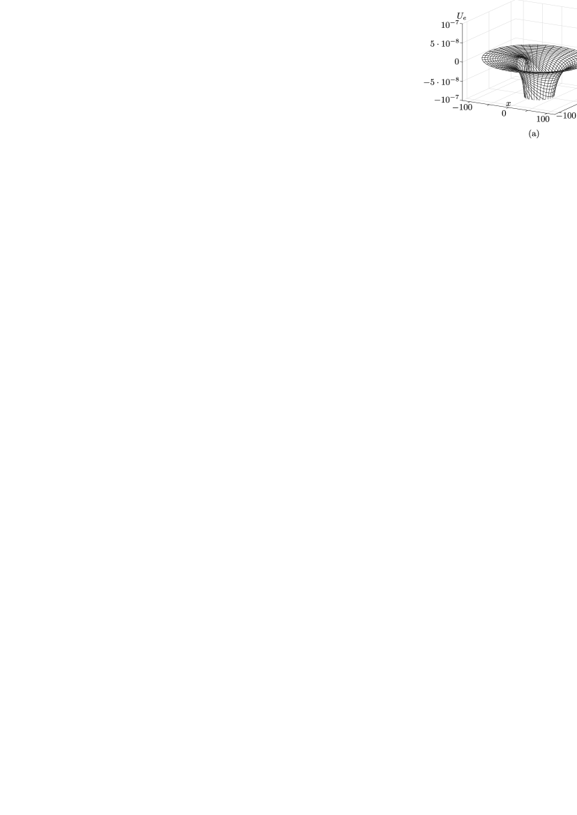
   Figure 5: A typical view of (a) the surface of the potential and (b) the profile of the function $U_{e}(x,\,0)$ for $|k|=k_{inf}\approx 0.81153$. The parameter values: $m_{c}=1$, $d=0.1$, $R=1$, $\rho=1$, $q=1$. The coordinate of the inflection point is $x_{inf}\approx-41.0591$

3. If $k_{inf}<|k|<k_{cr}$, the potential (47) has a maximum point and a saddle point on the negative part of the axis $Ox$ (see Fig. 6). Numerical analysis shows that the saddle point goes to minus infinity as $|k|\to k_{cr}-0$.

   

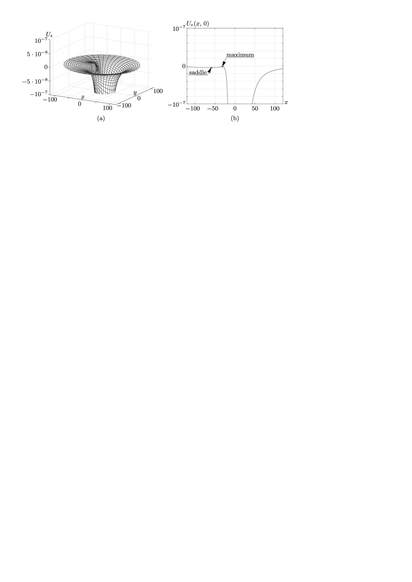
   Figure 6: A typical view of (a) the surface of the potential and (b) the profile of the function $U_{e}(x,\,0)$ for $k_{inf}<|k|<k_{cr}$. The parameter values: $m_{c}=1$, $d=0.1$, $R=1$, $\rho=1$, $q=1$, $k\approx 0.81156$, $k_{inf}\approx 0.81153$, $k_{cr}\approx 0.81188$. The coordinate of the saddle is $x_{s}\approx-59.09713$ and that of the maximum point is $x_{max}\approx-31.45989$

4. If $|k|=k_{cr}$, the potential (47) has only a maximum point, and the saddle point disappears. A typical view the surface of the potential and its profile in the plane $y=0$ are shown in Fig. 7.

   

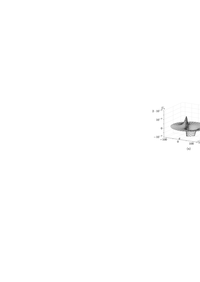
   Figure 7: A typical view of (a) the surface of the potential and (b) the profile of the function $U_{e}(x,\,0)$ for $|k|=k_{cr}\approx 0.81188$. The parameter values: $m_{c}=1$, $d=0.1$, $R=1$, $\rho=1$, $q=1$. The coordinate of the maximum point is $x_{max}\approx-20.54072$

5. If $k_{cr}<|k|$, the potential (47) has a maximum point on the negative part of the axis $Ox$ and a saddle point on the positive part of the axis (see Fig. 8). Numerical analysis shows that the saddle point goes to plus infinity as $|k|\to k_{cr}+0$.

   

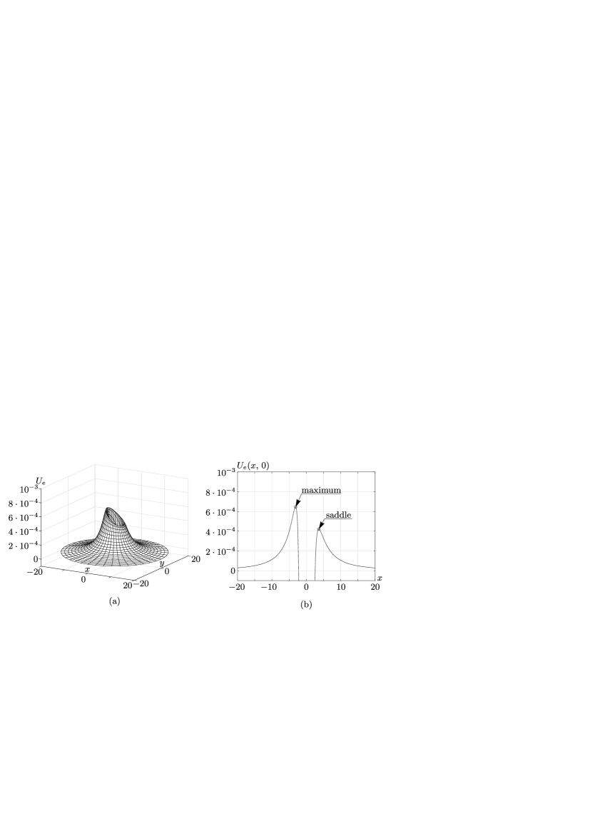
   Figure 8: A typical view of (a) the surface of the potential and (b) the profile of the function $U_{e}(x,\,0)$ for $|k|>k_{cr}\approx 0.81188$. The parameter values: $m_{c}=1$, $d=0.1$, $R=1$, $\rho=1$, $q=1$, $k\approx 0.86872$. The coordinate of the saddle is $x_{s}\approx 3.62443$ and that of the maximum point is $x_{max}\approx-3.11904$

The critical points of the effective potential $(x^{*},\,0)$ correspond to the fixed points of the reduced equations of motion: $x=x^{*}$, $y=0$, $\dot{x}=\dot{y}=0$. Here, by $x^{*}$ we mean the coordinate $x$ of any of the above-mentioned critical points. In this case, the trajectory of the center of the foil is a circle:

$$X_{c}(t)=x^{*}\cos\vartheta(t),\quad Y_{c}=x^{*}\sin\vartheta(t),\quad\vartheta(t)=\frac{kt}{m(x^{*})^{2}+2m_{c}dx^{*}+I_{c}+m_{c}d^{2}}.$$ (55)

We note that, since the critical points of the potential are either maximum points or saddle points, the motion in a circle (55) is unstable.

We have seen that the effective potential has no minimum points. In addition, numerical experiments show that the phase trajectories of the reduced system either go to infinity or “fall” on the source. Thus, we can formulate the following hypothesis:

1. In the system under consideration there exist no compact trajectories except for trajectories corresponding to the fixed points of the reduced system.

We now construct Hill’s regions for the case $|k|>k_{cr}$. For $0<h<U_{e}(x_{s},\,0)$ we have two Hill’s regions divided by the potential barrier (see Fig. 9a). Thus, for the above-mentioned level sets of the energy integral the trajectories from region $A$ never fall on the source, and the trajectories from region $B$ never go to infinity. When $h=U_{e}(x_{s},\,0)$, these regions come into contact with each other at the point $(x_{s},\,0)$, and when $h>U_{e}(x_{s},\,0)$, there is only one Hill’s region whose trajectories can both go to infinity and fall on the source (see Fig. 9b, c).

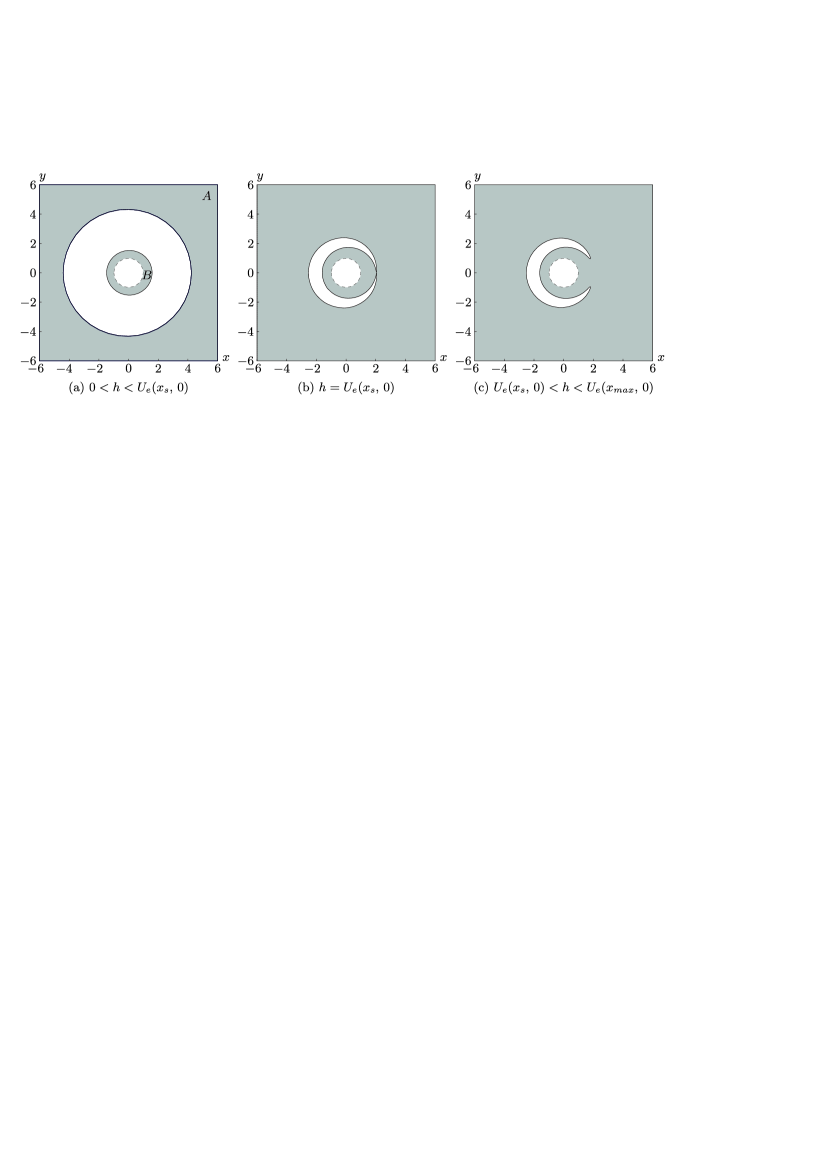
(a)                                             (b)                                             (c)

Figure 9: Hill’s regions for the case $|k|>k_{cr}$. The solid lines correspond to the boundaries of Hill’s regions, and the dashed line corresponds to a contact of the cylinder with the source.

4.2 Nonintegrability of the equations of motion

We show that equations (16) are nonintegrable. One of the classical numerical methods of investigating the nonintegrability of equations of motion is the method of constructing a Poincaré map [40]. However, such a map requires that the phase trajectory return to the secant. The analysis made in subsection 4.1 has shown that almost all trajectories of the system (16) are noncompact, except for a finite number of unstable periodic trajectories, which makes the traditional Poincaré map inapplicable. Nonetheless, the nonintegrability of equations (16) can be investigated using a scattering map, which is an analog of the Poincaré map for systems with noncompact trajectories [41].

We will consider the motion on the level sets of the integral (18) $|k|>k_{cr}$ and the levels of energy corresponding to the case shown in Fig. (9)a. The restrictions made are sufficient to ensure that the foil’s trajectories coming from infinitely remote points will not “fall” on the source, but go back to infinity.

To construct a scattering map, it is convenient to write the equations of motion (16) in the momenta relative to the rotating coordinate system $Oxy$. To do so, we make the change of variables (43)

$$x=X_{c}\cos\vartheta+Y_{c}\sin\vartheta,\quad y=-X_{c}\sin\vartheta+Y_{c}\cos\vartheta$$

and denote the new momenta:

$$p_{x}=(\Pi_{x}+A_{x})\cos\vartheta+(\Pi_{y}+A_{y})\sin\vartheta,\quad p_{y}=-(\Pi_{x}+A_{x})\sin\vartheta+(\Pi_{y}+A_{y})\cos\vartheta,\quad p_{\vartheta}=\Pi_{\vartheta}.$$ (56)

The change of variables (43) and (56) satisfies the relations

$$\boldsymbol{u}(x)=\boldsymbol{u}(y)=\boldsymbol{u}(p_{x})=\boldsymbol{u}(p_{y})=\boldsymbol{u}(p_{\vartheta})=0,\quad\boldsymbol{u}(\vartheta)=1,$$ (57)

where $\boldsymbol{u}$ is the symmetry field (19). Due to (57), the variable $\vartheta$ becomes cyclic and the equations for $x$, $y$, $p_{x}$, $p_{y}$ and $p_{\vartheta}$ decouple from the complete system of equations. In this case, the variable $\vartheta$ is necessary only to reconstruct the motion in the full phase space and need not be considered in the further analysis of integrability, see, e.g., [42].

In the new variables the Hamiltonian (17) becomes

$$H=\frac{1}{2}\left(\boldsymbol{p},\,\widetilde{\mathbb{Q}}^{-1}\boldsymbol{p}\right)-\frac{\rho q^{2}}{4\pi}\Bigl{(}\ln\bigl{(}x^{2}+y^{2}\bigr{)}-\ln\bigl{(}x^{2}+y^{2}-R^{2}\bigr{)}\Bigr{)},$$ (58)

$$\boldsymbol{p}=\begin{pmatrix}p_{x}\\ p_{y}\\ p_{\vartheta}\end{pmatrix},\quad\widetilde{\mathbb{Q}}=\begin{pmatrix}m&0&0\\ 0&m&m_{c}d\\ 0&m_{c}d&I_{c}+m_{c}d^{2}\end{pmatrix}.$$

We recall that $m=m_{c}+\rho\pi R^{2}$.

The nonzero Poisson brackets in the new variables have the form

$$\begin{gathered}\{p_{x},\,p_{\vartheta}\}=p_{y},\quad\{p_{y},\,p_{\vartheta}\}=-p_{x},\quad\{x,\,p_{x}\}=\{y,\,p_{y}\}=\{\vartheta,\,p_{\vartheta}\}=1,\\ \{x,\,p_{\vartheta}\}=y,\quad\{y,\,p_{\vartheta}\}=-x.\end{gathered}$$ (61)

The integral (18) in the new variables preserves its form:

$$K=p_{\vartheta}+p_{y}x-p_{x}y=\mathrm{const}\,.$$ (62)

On the fixed level set $K=k$ of the first integral (62) the variable $p_{\vartheta}$ can be eliminated from the equations of motion. In addition, to analyze the dynamics, it is more convenient to make another change of variables:

$$x=r\cos\varphi,\quad y=r\sin\varphi,\quad p_{x}=p\cos\alpha,\quad p_{y}=p\sin\alpha.$$ (63)

The reduced system of equations of motion can be represented as

$$\begin{gathered}\dot{r}=m^{-1}p\cos(\alpha-\varphi)-m^{-1}m_{c}d\sin\varphi\Omega,\quad\dot{\varphi}=\frac{p\sin(\alpha-\varphi)}{mr}-\frac{m_{c}d\cos\varphi}{mr}\Omega-\Omega,\\ \dot{p}=-\frac{\rho q^{2}R^{2}}{2\pi}\frac{\cos(\alpha-\varphi)}{r(r^{2}-R^{2})},\quad\dot{\alpha}=\frac{\rho q^{2}R^{2}}{2\pi}\frac{\sin(\alpha-\varphi)}{r(r^{2}-R^{2})p}-\Omega,\end{gathered}$$ (66)

$$\Omega=\frac{k-rp\sin(\alpha-\varphi)-m^{-1}m_{c}dp\sin\alpha}{I_{c}+m_{c}d^{2}-m^{-1}m_{c}^{2}d^{2}},$$ (67)

with the Hamiltonian

$$H=\frac{1}{2}\left(m^{-1}p^{2}+(I_{c}+m_{c}d^{2}-m^{-1}m_{c}^{2}d^{2})\Omega^{2}\right)+\frac{\rho q^{2}}{4\pi}\ln\left(1-\frac{R^{2}}{r^{2}}\right)$$ (68)

and the Poisson bracket

$$\begin{gathered}\{r,\,p\}=\cos(\varphi-\alpha),\quad\{r,\,\alpha\}=\frac{\sin(\varphi-\alpha)}{p},\\ \{\varphi,\,p\}=-\frac{\sin(\varphi-\alpha)}{r},\quad\{\varphi,\,\alpha\}=\frac{\cos(\varphi-\alpha)}{rp},\quad\{\vartheta,\,K\}=1.\end{gathered}$$ (71)

We see that the equations in the variables $r$, $\varphi$, $p$ and $\alpha$ decouple from the complete system and possess the first integral (68). Equation (67) and the first integral (62) are necessary to reconstruct the motion in the complete phase space of the system.

We note that the terms with $\dot{\vartheta}$ arise in equations (66) due to transformation to the moving coordinate system and lead to a drift in the system. In fact, we have the problem of a material point moving on the surface of a potential rotating with angular velocity $-\dot{\vartheta}$.

From the form of equations (66) and the Hamiltonian (68) it can be seen that, as $r\to\infty$, the following holds:

$$\begin{gathered}b=r\sin(\alpha-\varphi)+m^{-1}m_{c}d\sin\alpha\to\mathrm{const}\,,\quad\dot{\vartheta}\to\mathrm{const}\,,\\ \alpha-\varphi\to\pi n,\quad\alpha+\vartheta\to\mathrm{const}\,,\quad\varphi+\vartheta\to\mathrm{const}\,,\quad p\to\mathrm{const}\,.\end{gathered}$$ (74)

Thus, as the foil recedes to a sufficiently great distance from the source, the foil rotates almost uniformly with angular velocity $\dot{\vartheta}$. In (74) the quantity $b$ has the meaning of an impact parameter.

In order to demonstrate the nonintegrability of equations (66), we construct a scattering map, as is done in [41]. This map is a composition of two maps: a direct map $\mathcal{F}$ and a feedback map $\mathcal{B}$.

1. The direct map $\mathcal{F}$ consists in integrating equations (66) with the initial condition $(r_{max},\,\varphi_{k},\,p_{k},\,\alpha_{k})$. In this case, the hypersurface $r=r_{max}$ is a secant of the scattering map, and the value of momentum $p_{k}$ is calculated from a given level of energy and the values $r_{max}$, $\varphi_{k}$ and $\alpha_{k}$. We note that, since the Hamiltonian (68) is a quadratic function of momentum $p$, there exist on each fixed level of energy two different values of momentum $p$. As $p_{k}$ we need to choose solely either the largest or the smallest value of momentum.

   Integration of equations (66) is performed until the phase trajectory reaches again the secant $r=r_{max}$ (see Fig.10). We denote the end point as $(r_{max},\,\varphi_{k}^{e},\,p_{k}^{e},\,\alpha_{k}^{e})$. It should be kept in mind that, regardless of the choice of the initial momentum, the value $p_{k}^{e}$ can correspond both to the largest and to the smallest of the possible values of momentum.

2. The feedback map (see Fig. 10) consists in transforming the final values of the angle variables $\alpha_{k}^{e}$ and $\varphi_{k}^{e}$ to the new initial values as follows:

   $$\alpha_{k+1}=\alpha_{k}^{e},\quad\varphi_{k+1}=2\alpha_{k}^{e}-\varphi_{k}^{e}+\pi.$$ (75)

Applying alternately the direct map $\mathcal{F}$ and the feedback map $\mathcal{B}$, we obtain the following two-dimensional map:

$$\mathcal{B}\mathcal{F}:\ (\varphi_{k},\,\alpha_{k})\to(\varphi_{k+1},\,\alpha_{k+1}).$$ (76)

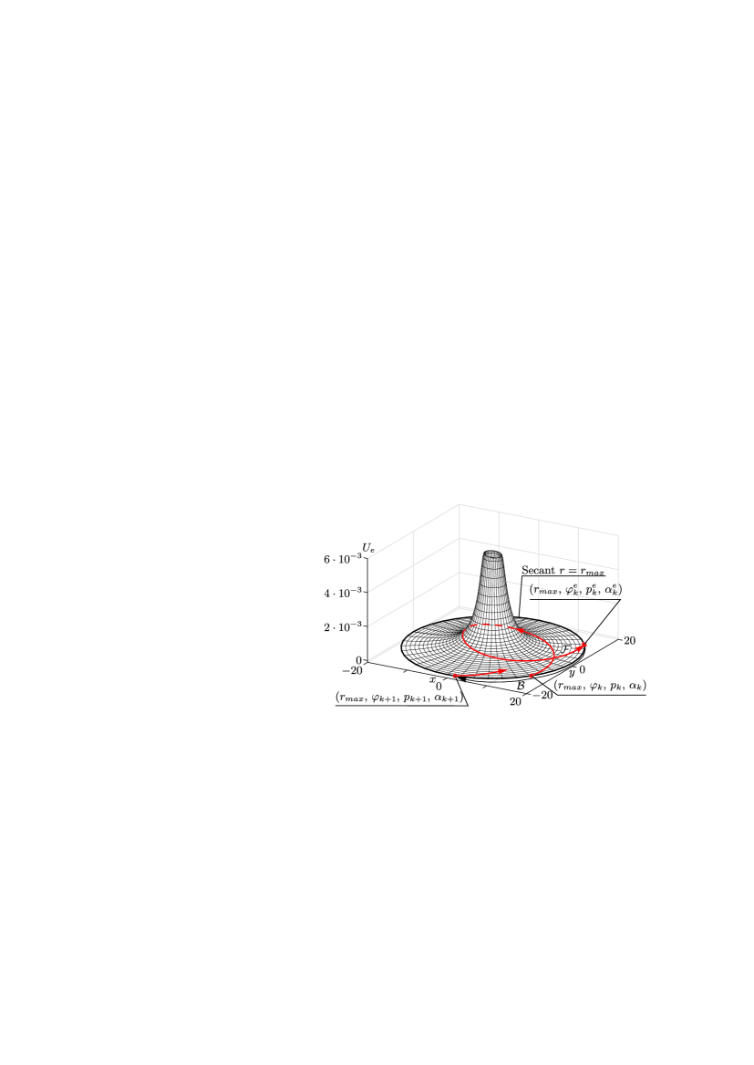
Figure 10: A schematic illustration of a scattering map. $\mathcal{F}$ is the direct map and $\mathcal{B}$ is the feedback map

We note that, by virtue of the properties (74) of the reduced system, the map (76) may be visualized more conveniently by passing from the angle $\varphi$ to the impact parameter:

$$b=r\sin(\alpha-\varphi)+m^{-1}m_{c}d\sin\alpha,$$ (77)

whose value tends, as $r$ increases, to a constant value in contrast to the angle $\varphi$. An example of a scattering map on the plane $(\alpha,\,b)$ is shown in Figs. 11 and 12

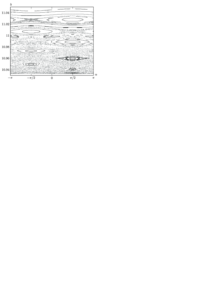
Figure 11: The parameter values $m_{c}=1$, $\rho=1$, $d=0.01$, $I_{c}=1$, $R=1$, $k=1$, $q=1$, $h=0.001$, $r_{max}=100$. As the initial momentum we have chosen the largest value.

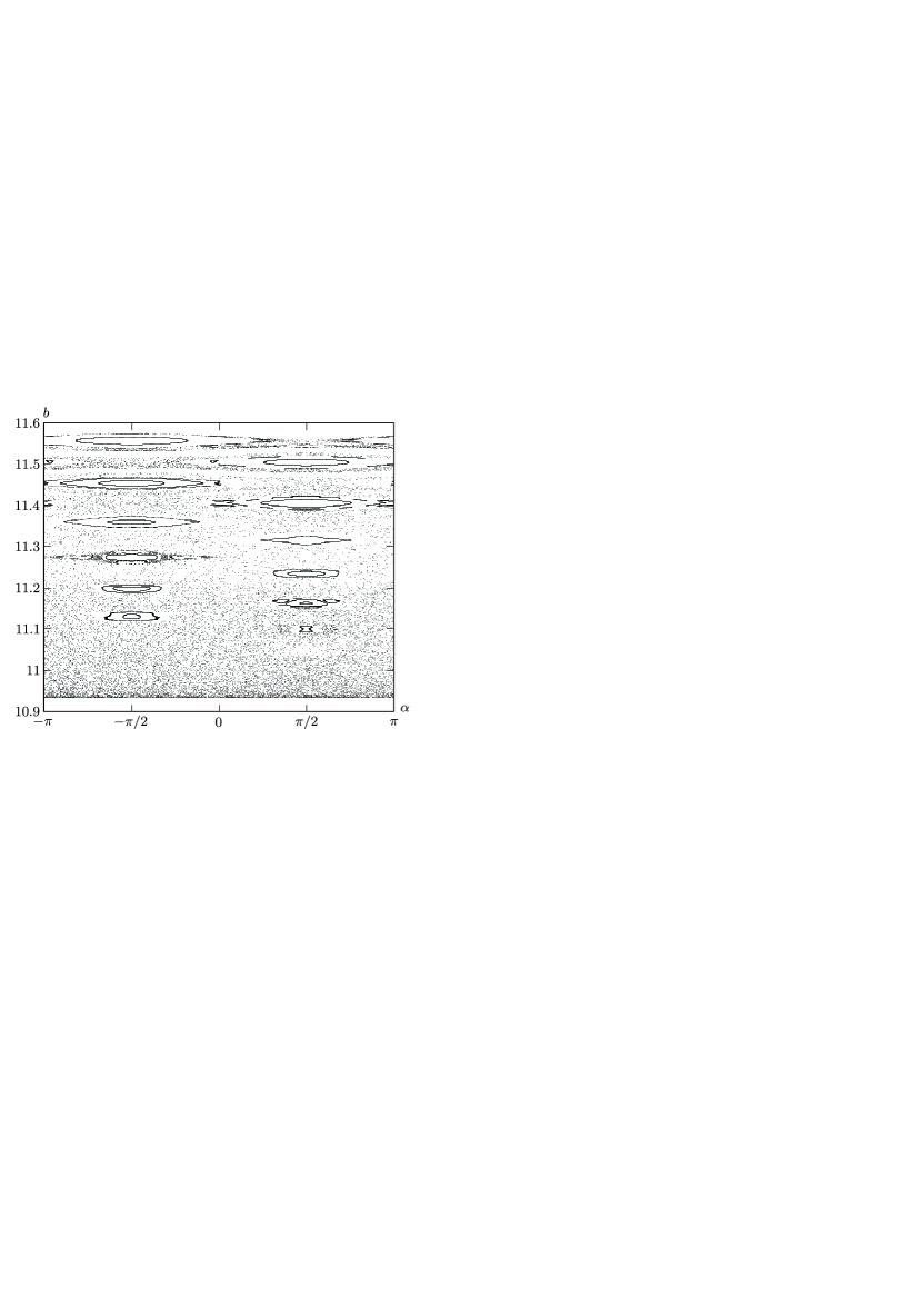
Figure 12: The parameter values $m_{c}=1$, $\rho=1$, $d=0.01$, $I_{c}=1$, $R=1$, $k=1$, $q=1$, $h=0.001$, $r_{max}=100$. As the initial momentum we have chosen the smallest value.

Figures 11 and 12 shows invariant curves and chaotic regions similar to the classical Poincaré maps. In the case of a balanced circular foil ($d=0$) the phase space of the scattering map is foliated by invariant curves $b=\mathrm{const}\,$.

We note that, at large values of $r_{max}$, the portrait of the scattering map changes visually due to the drift of the variable $\alpha$ (see Fig. 13).

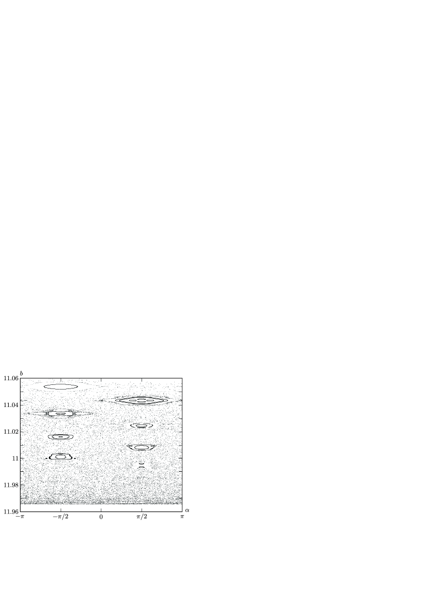
Figure 13: The parameter values $m_{c}=1$, $\rho=1$, $d=0.01$, $I_{c}=1$, $R=1$, $k=1$, $q=1$, $h=0.001$, $r_{max}=200$. As the initial momentum we have chosen the largest value.

The question remains open whether nonintegrability with a given $r_{max}$ implies nonintegrability for any values of $r$. Thus, the constructed scattering maps allow the following hypothesis to be formulated:

1. The equations of motion (16) of an unbalanced circular foil in the field of a fixed source of constant intensity are nonintegrable.

Remark 8.

Constructing a scattering map requires a multiple integration of equations (66) by some numerical method for a long physical time interval. Since the system considered is Hamiltonian, the scattering map cannot contain any attracting or repelling sets. Nevertheless, when one uses explicit Runge – Kutta methods, the map may exhibit, in particular, asymptotically stable fixed points. This is due to the fact that long integration leads to a distortion of the level set of the energy integral (68). For this reason, for numerical integration we have used two types of methods: projection methods, which return the system’s trajectory to the level surface of the integral (68) at the end of each step of integration, and collocation methods, which are symplectic and guarantee preservation of the phase volume with some accuracy [43]. Both methods lead to visually similar results. However, projection methods are more efficient in terms of CPU time expenditures, since they can be based on any explicit method, whereas collocation methods are completely implicit and require solving a nonlinear system of algebraic equations on each step of integration.

References

- [1] Helmholtz H. über integrale hydrodinamischen gleichungen welche den wirbelbewegungen entsprechen // J. rein. angew. Math. — 1858. — Bd. 55. — S. S. 25 – 55.
- [2] Kirchhoff G. Vorlesungen über mathematische Physik. — Leipzig: Mechanik, 1874.
- [3] Ziglin S. L. Nonitegrability of the problem of the motion of four point vortices // Dokl. Akad. Nauk SSSR. — 1980. — Vol. 250, no. 6. — P. 1296 – 1300.
- [4] Borisov A. V., Kilin A. A., Mamaev I. S. Transition to chaos in dynamics of four point vortices on a plane // Doklady Physics. — Vol. 51, no. 5.
- [5] Kurakin L. G., Yudovich V. I. The stability of stationary rotation of a regular vortex polygon // Chaos: An Interdisciplinary Journal of Nonlinear Science. — 2002. — Vol. 12, no. 3. — P. 574 – 595.
- [6] Borisov A. V., Kilin A. A. Stability of thomson’s configurations of vortices on a sphere // Regular and Chaotic Dynamics. — 2000. — Vol. 5, no. 2. — P. 189 – 200.
- [7] Borisov A. V., Mamaev I. S., Bizyaev I. A. Three vortices in spaces of constant curvature: Reduction, poisson geometry, and stability // Regular and Chaotic Dynamics. — 2018. — Vol. 23, no. 5. — P. 613 – 636.
- [8] Kurakin L. G. Stability, resonances and instability of regular vortex polygons inside a circular region // Doklady Physics. — 2004. — Vol. 49, no. 11. — P. 658 – 661.
- [9] Borisov A. V., Mamaev I. S. Mathematical methods in the dynamics of vortex structures. — Moscow–Izhevsk: Institute of Computer Science, 2005.
- [10] Vetchanin E. V., Kazakov A. O. Bifurcations and chaos in the dynamics of two point vortices in an acoustic wave // International Journal of Bifurcation and Chaos. — 2016. — Vol. 26, no. 4. — P. 1650063, 13 pp.
- [11] Vetchanin E. V., Mamaev I. S. Dynamics of two point vortices in an external compressible shear flow // Regular and Chaotic Dynamics. — 2017. — Vol. 22, no. 8. — P. 893 – 908.
- [12] Dynamics of vortex dipoles in confined bose–einstein condensates / P J Torres, P G Kevrekidis, D J Frantzeskakis et al. // Physics Letters A. — 2011. — Vol. 375. — P. 3044 –– 3050.
- [13] Koukouloyannis V., Voyatzis G., Kevrekidis P. G. Dynamics of three noncorotating vortices in bose – einstein condensates // Physical Review E. — 2014. — Vol. 89. — P. 042905.
- [14] Ryabov P. E., Sokolov S. V. Phase topology of two vortices of identical intensities in a bose – einstein condensate // Russian Journal of Nonlinear Dynamics. — 2019. — Vol. 15, no. 1. — P. 59 –– 66.
- [15] -symmetric interaction of hetons. i. analysis of the case / M A Sokolovskiy, K V Koshel, D G Dritschel, Reinaud J N // Physics of Fluids. — 2020. — Vol. 32, no. 9. — P. 096601.
- [16] Sokolovskiy M. A., Carton X. J., Filyushkin B. N. Mathematical modeling of vortex interaction using a three-layer quasigeostrophic model. part 1: Point-vortex approach // Mathematics. — 2020. — Vol. 8, no. 8. — P. 1228.
- [17] Blackmore D., Knio O. Transition from quasiperiodicity to chaos for three coaxial vortex rings // ZAMM Z. Angew. Math. Mech. — 2000. — Vol. 80, no. S1. — P. 173 – 176.
- [18] Blackmore D., Knio O. Kam theory analysis of the dynamics of three coaxial vortex rings // Physica D: Nonlinear Phenomena. — 2000. — Vol. 140, no. 3-4. — P. 321 – 348.
- [19] Borisov A. V., Kilin A. A., Mamaev I. S. The dynamics of vortex rings: Leapfrogging, choreographies and the stability problem // Regular and Chaotic Dynamics. — 2013. — Vol. 18, no. 1-2. — P. 33 – 62.
- [20] The dynamics of vortex rings: leapfrogging in an ideal and viscous fluid / A V Borisov, A A Kilin, I S Mamaev, V A Tenenev // Fluid Dynamics Research. — 2014. — Vol. 46, no. 3. — P. 031415, 16 pp.
- [21] Ramodanov S. M. Motion of a circular cylinder and a vortex in an ideal fluid // Regular and Chaotic Dynamics. — 2001. — Vol. 6, no. 1. — P. 33 – 38.
- [22] Ramodanov S. M. Motion of a circular cylinder and point vortices in a perfect fluid // Regular and Chaotic Dynamics. — 2002. — Vol. 7, no. 3. — P. 291 – 298.
- [23] The hamiltonian structure of a two-dimensional rigid circular cylinder interacting dynamically with point vortices / B N Shashikanth, J E Marsden, J W Burdick, S D Kelly // Physics of Fluids. — 2002. — Vol. 14, no. 3. — P. 1214 – 1227.
- [24] Mamaev I. S., Bizyaev I. A. Dynamics of an unbalanced circular foil and point vortices in an ideal fluid // Physics of Fluids. — 2021. — Vol. 33. — P. 087119, 18 pp.
- [25] Mason R. J. Fluid locomotion and trajectory planning for shape-changing robots : Phd dissertation / R J Mason ; Pasadena, California: California Institute of Technology.
- [26] Michelin S., Smith S. G. L. An unsteady point vortex method for coupled fluid-solid problems // Theor. Comput. Fluid Dyn. — 2009. — Vol. 23, no. 2. — P. 127 – 153.
- [27] Fedonyuk V., Tallapragada P. The dynamics of a chaplygin sleigh with an elastic internal rotor // Regular and Chaotic Dynamics. — 2019. — Vol. 24, no. 1. — P. 114 – 126.
- [28] Fridman A. A., Y P. P. On moving singularities of a flat motion of an incompressible fluid // Geofiz. Sbornik. — 1928. — P. 9 – 23.
- [29] S.G. L. S. How do singularities move in potential flow? // Physica D: Nonlinear Phenomena. — 2011. — Vol. 240, no. 20. — P. 1644 – 1651.
- [30] Bizyaev I. A., Borisov A. V., Mamaev I. S. The dynamics of three vortex sources // Regular and Chaotic Dynamics. — 2014. — Vol. 19, no. 6. — P. 694 – 701.
- [31] Bizyaev I. A., Borisov A. V., Mamaev I. S. The dynamics of vortex sources in a deformation flow // Regular and Chaotic Dynamics. — 2016. — Vol. 21, no. 3. — P. 367 – 376.
- [32] Artemova E. M., Vetchanin E. V. Control of the motion of a circular cylinder in an ideal fluid using a source // Bulletin of Udmurt University. Mathematics. Mechanics. Computer Science. — 2020. — Vol. 30, no. 4. — P. 604 – 617.
- [33] Kochin N. E., Kibel I. A., Roze N. V. Theoretical Hydrodynamics. — New York: Wiley, 1964.
- [34] Milne-Thomson L. M. Theoretical hydrodynamics. — 4th ed. edition. — Macmillan & Co. Ltd, 1962.
- [35] Sedov L. I. Ploskie zadachi gidrodinamiki i aerodinamiki (Two-dimensional problems in hydro- and aeromechanics). — Second edition edition. — Moscow: Gostekhizdat, 1950.
- [36] Korotkin A. I. Added Masses of Ship Structures. — Springer, Dordrecht, 2009. — Vol. 88 of Fluid Mech. Appl.
- [37] Bizyaev I. A., Mamaev I. S. Dynamics of a pair of point vortices and a foil with parametric excitation in an ideal fluid // Bulletin of Udmurt University. Mathematics. Mechanics. Computer Science. — 2020. — Vol. 30, no. 4. — P. 618 – 627.
- [38] Arnold V. I. Ordinary Differential Equations. — Berlin: Springer, 2006.
- [39] Bolsinov A. V., Borisov A. V., Mamaev I. S. Topology and stability of integrable systems // Russian Mathematical Surveys. — Vol. 65, no. 2.
- [40] Kuznetsov S. P. Dynamical Chaos (lecture course). — 2nd ed. edition. — Moscow: Fizmatlit, 2006.
- [41] Jung C. Poincaré map for scattering states // Journal of physics A: mathematical and general. — 1986. — Vol. 19, no. 8. — P. 1345 – 1353.
- [42] Borisov A. V., Mamaev I. S. Symmetries and reduction in nonholonomic mechanics // Regular and Chaotic Dynamics. — 2015. — Vol. 20, no. 5. — P. 553 – 604.
- [43] Hairer E., Lubich C., Wanner G. Geometric Numerical Integration: Structure-Preserving Algorithms for Ordinary Differential Equations. — New York: Springer, 2006. — Vol. 31 of Springer Ser. Comput. Math.