Experience feedback using Representation Learning for Few-Shot Object Detection on Aerial Images

Abstract

This paper proposes a few-shot method based on Faster R-CNN and representation learning for object detection in aerial images. The two classification branches of Faster R-CNN are replaced by prototypical networks for online adaptation to new classes. These networks produce embeddings vectors for each generated box, which are then compared with class prototypes. The distance between an embedding and a prototype determines the corresponding classification score. The resulting networks are trained in an episodic manner. A new detection task is randomly sampled at each epoch, consisting in detecting only a subset of the classes annotated in the dataset. This training strategy encourages the network to adapt to new classes as it would at test time. In addition, several ideas are explored to improve the proposed method such as a hard negative examples mining strategy and self-supervised clustering for background objects. The performance of our method is assessed on DOTA, a large-scale remote sensing images dataset. The experiments conducted provide a broader understanding of the capabilities of representation learning. It highlights in particular some intrinsic weaknesses for the few-shot object detection task. Finally, some suggestions and perspectives are formulated according to these insights.

1 Introduction

Object detection is a key problem in computer vision. It consists in finding all occurrences of objects belonging to a predefined set of classes in an image and classify them. Its applications range from medical diagnosis to aerial intelligence through autonomous vehicles. Object detection methods automate repetitive and time-consuming tasks performed by human operators until now. In the context of Remote Sensing Images (RSI), detection is used for a wide variety of tasks such as environmental surveillance, urban planning, crops and flock monitoring or traffic analysis.

Deep learning and especially convolutional neural networks (CNNs) outperform previous methods on most computer vision tasks and object detection is no exception. Plenty of methods have been introduced to address this challenge. Among them, Faster R-CNN [1] and YOLO [2] may be the most well-known and studied. Even though this problem is far from being solved, detection algorithms perform well when provided with sufficient annotated data. However, this is often not available in practice and the creation of large dataset for detection requires both time and expertise preventing the deployment of such methods for many use cases. Another limitation to the widespread deployment of detection techniques is the lack of adaptability. Once fully trained, it is hard to modify a model to adapt to new objects. This is critical for some applications which need to detect different objects from one usage to another. Aerial intelligence is an example of such application: each mission may have its specific objects of interest and therefore a detection model must be adaptable (literally) on the fly. The overall objective of this work is to be deployed on vertical aerial images. Yet, large-scale dataset of such images, annotated for object detection, are rare. RSI are a convenient alternative and provide an accurate estimation of performance in deployment.

Few-Shot Learning (FSL) techniques have been introduced to address these issues and deal with limited data. This has been extensively studied for classification [3], [4]. Its principle is to learn general knowledge from a large dataset so that it can generalize efficiently (i.e. quickly and from limited data) on new classes. There exist different approaches for this task. Representation learning tries to learn abstract embeddings of images so that the representation space is semantically organized in a way that makes classification relatively easy (e.g. with a linear classifier). Meta-learning based methods learn a model (teacher) that helps another model (student) to perform well based on a limited amount of data. This is often done by training both network on multiple low-data tasks (e.g. by changing classes between epochs). Transfer learning is also a valid approach for FSL. It consists in training a model on a large dataset and then adapt it to perform well on another smaller one. This requires a supplementary training step and is often subject to catastrophic forgetting [5], and overfitting. It needs advanced tricks to prevent these undesirable effects.

This performs relatively well for classification but the more challenging detection task still lacks few-shot alternatives. Though, recent work focused on Few-Shot Object Detection (FSOD) applying ideas from FSL literature to object detection. The first approaches were mostly oriented toward transfer learning and fine-tuning [6, 7] disregarding the others FSL practices. Some other work took inspiration from meta-learning [8] and representation learning [9]. This is mostly applied to natural images, yet applications on remote sensing images are scarce [10, 11]. Even if object detection is hard, applying it on remote sensing images is even harder: object’s sizes can vary greatly plus they can be arbitrarily oriented and densely packed. These supplementary difficulties might explain why this specific topic remains mainly untouched.

This work introduces a new few-shot learning method for object detection and evaluates its performance on aerial images. It detects objects from only a few examples of a class and without any fine-tuning. The main idea is inspired from prototypical networks [3] which learns an embedding function that maps images into a representation space. Prototypes are computed from the few examples available for each class and classification scores are attributed to each input image according to the distances between its embedding and the prototypes. The classic Faster R-CNN framework is modified to perform few-shot detection based on this idea. Both classification branch in Region Proposal Network (RPN) and in Fast R-CNN are replaced by prototypical networks to allow fast online adaptation. In addition, a few improvements are introduced on the prototypical baseline in order to fix its weaknesses.

This paper begins with a brief overview of literature on object detection, few-shot learning and the intersection of these two topics. Then the prototypical Faster R-CNN architecture is presented in detail alongside with several improvements on our baseline. Next, the potential of the proposed modifications throughout a series of experiences is demonstrated. Finally, the proposed approach is discussed with a critical eye, and it is asked whether representation learning is suitable for object detection.

2 Related work

2.1 Object detection

During the last decade, deep learning and especially CNN have made impressive progresses in most computer vision tasks. Object detection is no exception and plenty of CNN based methods were proposed to address this problem. Among the most common, YOLO [2] is a one-stage method with a trade-off on speed. Faster R-CNN [1] is another well-known object detection technique that focuses more on accuracy with two separate stages. Most subsequent methods are more or less inspired from these. A common feature between these techniques is the generation of anchor boxes. These are bounding boxes chosen with different aspect ratios and sizes, uniformly distributed on the image, that the networks take as reference for the regression. Recently, some works tend to reduce the accuracy gap between one and two stages methods. Especially, FCOS [12] drops completely the anchors to build a fully convolutional one stage object detection network that matches the performance of Faster R-CNN.

As our work is mainly based on Faster R-CNN, we will describe its functioning in details. As mentioned above, it is made of two stages: a Region Proposal Network (RPN) and a prediction head described in [13]. A third component must also be mentioned, the backbone. This is a large CNN that extracts features from images. It is often chosen as a ResNet [14] with a Feature Pyramidal Network (FPN) [15] on top. This extracts features from different levels and is very helpful for detecting objects of various sizes. Once the features are extracted, they are fed into the RPN. This network is fully convolutional and will output an objectness score $o_{a}$ for each generated box $a$ (i.e. generally 3 boxes per positions in the multi-level feature map). This score represents the likeliness of having an object within the corresponding patch in the image. In addition, the RPN outputs box regressions $b_{a}^{\text{R}}$. The regressions, combined with the anchors sizes and positions, give the actual boxes coordinates in the image. Then, the best scoring boxes are selected to be fed to the prediction head, where boxes are refined and classified. For each box, the corresponding features are selected through a pooling operation (RoI Align, proposed by [16]). These are flattened and passed to the second stage. It computes refining coordinates shifts $b_{j}^{\text{H}}$ and classes scores $c_{j}$ for each box. Following this, a post-processing step filters out small, low-scoring and redundant boxes.

The training of this method is straightforward, each network has two losses, one for the regression branch and one for the classification as described below:

$$\mathcal{L}_{reg}^{\text{R}}(b_{i}^{\text{R}},\hat{b}_{i}^{\text{R}}) =\text{SmoothL1Loss}(b_{i}^{\text{R}},\hat{b}_{i}^{\text{R}}),$$ (1)

$$\mathcal{L}_{obj}^{\text{R}}(o_{i},\hat{o}_{i}) =\hat{o}_{i}\log(o_{i})+(1-\hat{o}_{i})\log(1-o_{i}),$$ (2)

$$\mathcal{L}_{reg}^{\text{H}}(b_{j}^{\text{H}},\hat{b}_{j}^{\text{H}}) =\text{SmoothL1Loss}(b_{j}^{\text{H}},\hat{b}_{j}^{\text{H}}),$$ (3)

$$\mathcal{L}_{cls}^{\text{H}}(c_{j},\hat{c}_{j}) =-\log(c_{j}),$$ (4)

where SmoothL1loss is a slight modification to L1 error function. Below a certain threshold, the error is computed according to L2 loss, while above that threshold L1 is used. This penalizes the network less for small errors in boxes regressions. The variables with hat correspond to ground truth values. These losses are combined in an overall objective function that is optimized using stochastic gradient descent:

$$\mathcal{L}=\mathcal{L}_{reg}^{\text{R}}+\mathcal{L}_{obj}^{\text{R}}+\mathcal{L}_{reg}^{\text{H}}+\mathcal{L}_{cls}^{\text{H}}.$$ (5)

During training, not all boxes are selected for computing losses. First, the generated boxes are separated into two groups: positive examples, i.e. boxes with an overlap of at least 0.7 with a ground truth annotation, and negative examples which represent the background class. Positive and negatives examples are included in classification losses computation while only positives are for regression.

2.2 Few-shot learning

Few-shot learning corresponds to learning a task in a limited data setting. Specifically, a task is defined as $K$-shots, $N$-ways learning when the training set only contains $K$ examples for each of its $N$ classes. In FSL literature, it is common to introduce the query and support sets for a given task. The support contains the available examples: $K$ images for each of the $N$ classes of the task. It can be seen as the training set for that task. The query set contains images from the same classes as the support and is used for assessing the performance of the model, like a test set.

There exists different techniques to tackle low data regime. Transfer learning is one of them. It consists in training a network on a large-scale dataset (source domain) and then fine-tuning it on the few examples (target domain) available for the actual task. This kind of methods require re-training each time a new class is added. In the case of aerial surveillance, this is not suitable as the adaptability must be almost immediate. In addition, these techniques are often inclined to catastrophic forgetting [5], a recurrent problem in continual learning. Classes previously learned are forgotten when learning to classify new classes. Therefore, we will only discuss in this paper methods based on meta learning or representation learning.

Meta-learning, in the context of FSL, refers to methods that train a model called the meta-learner whose task will be to help another model to train efficiently (in terms of computation and data) for the actual problem. This can be pictured as training a teacher model whose goal is to make its student learn better. That way, the student can quickly learn new tasks and perform well in low-data regime. Meta-learning methods often share the same training strategy with two nested optimization loops. The inner one updates the weights of the student net, while the outer one deals with the meta-learner. Between each iteration of the outer loop, a new task is chosen for the inner network to learn. The student is trained on the support set while the teacher’s objective is to maximize the student performance. Many ways of teaching were introduced. For instance, the teacher network can be trained to directly output weight updates of the student as described in [4]. Another approach is to output only initial weights for the student as in [17]. The starting point is hopefully better than random, thus allowing faster and better optimization. While these techniques are promising, they do not scale very well for large networks as the teacher must be substantially larger than the learner. In order to assess generalization performance, classes are split into two categories: base and novel classes (or equivalently seen and unseen classes). During meta-training, tasks are sampled using only base classes. At test time, however they can be sampled either from novel classes or both base and novel.

Another drawback is the necessary fine-tuning. Even if it should be quicker than regular transfer learning, most meta-learning methods still require this additional step. Some exceptions are based on representation learning or metric learning. The principle is to train a network to output an abstract representation from an input image. This is first introduced for signature verification with siamese networks in [18]. Prototypical networks [3] is a pioneer work in using this for FSL. An embedding network is trained to produce such representations. Before inference, prototypes for each class are computed using the embedding net and the support images. During inference, the query images are embedded and the distance between their representations and the prototypes determine the classification scores. In [3], this is done with a linear classifier, but other choices are possible. Relation networks [19] proposes another network to compute the class scores from the image representation and the prototypes. Similarly, matching networks [20] used two separate networks to embed the image and the prototypes. These methods are usually trained by randomly sampling tasks at each epoch, just as other meta-learning methods. This succession of new tasks helps the network to generalize well and therefore improves its accuracy on unseen classes.

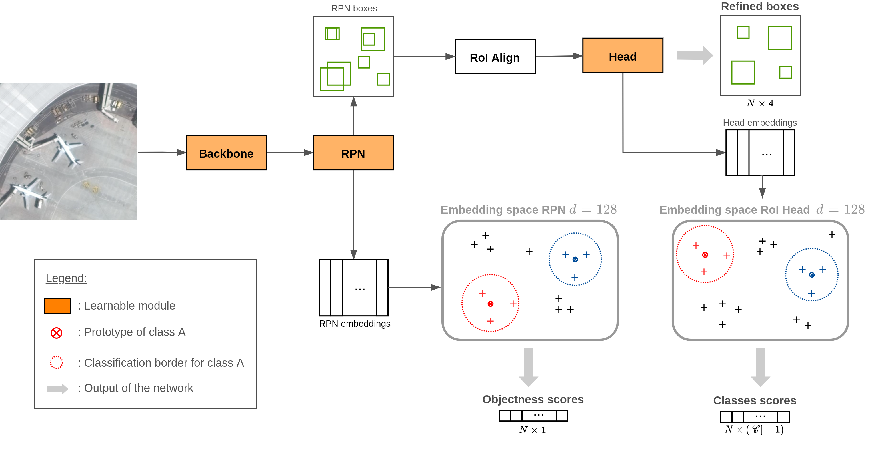
Figure 1: Architectural view of prototypical Faster R-CNN. Embedding vectors for each of the possible box locations is generated by the RPN. These are compared with class prototypes to output objectness scores. The same process occurs in the second stage to produce classes scores.

2.3 Few shot object detection

The focus of FSL was previously on classification tasks. Detection is a harder problem and so is FSL. That explains why the combination of both was only studied recently. One early work on this problem is Low-Shot Transfer Detector [6]. It applies few-shot transfer learning in order to refine a pre-trained detection network on a small dataset. To do so, they introduce two regularization losses during the fine-tuning phase. One forces the network to focus on new objects by reducing the magnitude of the feature maps on background areas. The other loss prevents forgetting knowledge from the source domain. It penalizes the refined network to have dissimilar activation in the pre-softmax layer compared to the network trained on base classes only. Similarly, [7] proposes to first pre-train a Faster R-CNN on a base dataset and then fine-tune only the last classification and regression layers with the new classes. This is quite similar to [6], but even simpler as it does not need any new loss functions.

Even if RepMet [9] focuses mostly on few-shot classification, authors showed that their method can also be applied for detection. Their approach is mainly based on metric learning. During base training, they learn alongside the network’s weights a set of representatives for different classes (several per class). These high-dimensional vectors define the centers of Gaussian distributions inside the embedding space. The class probabilities are assigned from the distances between the embedding vectors and the representatives in an analogous way as in [3]. At test time, the encoding network generates representatives from the few examples in dataset, which are then fine-tuned for a few iterations. For detection, they replace the second stage of Faster R-CNN with their classification module. Although this method is astride on meta-learning and representation learning it does not leverage an episodic task training strategy. Instead, it relies on fine-tuning: it trains first on base classes and fine-tune on novel ones. To our knowledge, this is the first attempt to solve FSOD with metric learning.

Most recent work focuses on meta-learning in order to solve FSOD. For instance, [21] trains a one stage detector along with a meta features extractor. This extractor is a CNN that computes a reweighting vector for each class from the support set. When a query image is passed through the detector, the features maps output by the backbone are channel-wise multiplied with the reweighting vectors to produce class-specific maps. These maps are then passed to the detector’s head. Each map is responsible for detecting objects of the corresponding class. Closely related, [8] incorporates a similar reweighting scheme in Faster R-CNN. A major difference though is that the features and reweighting vectors are computed with the same network. A similar class-attention mechanism, but inside the RPN network is proposed by [22]. In the second stage they use multi-relation heads that combine support set information and query image features in multiple ways inside the classification branch. Another attempt to leverage an attention mechanism is proposed by [23]. Query and support examples are co-adapted to reduce features discrepancies and improve prediction both in RPN and second stage. Except the latter, these methods are trained episodically.

Different methods for combining support information with the query features exist, e.g. [11] creates a graph between the support vectors and the query embeddings. Then a GRU [24] processes it in order to provide attention between regions of interest and support set images. Alike this, [25] processes a graph, whose final nodes are the reweighting vectors, with a graph convolution network. The graph is initialized with similarities between classes’ names, embedded with GloVe [26].

With regard to FSOD on remote sensing images, very few methods exist. To the best of our knowledge, only two works have been published on this topic. [10] improves on [21] by using an improved version of YOLO. This mainly adds multi-scale features and predictions. This is especially important to tackle RSI as object size can vary greatly. The second one [11], makes use of a two-stages detector and compute reweighting vectors with a GRU relation module. Both of the methods provide benchmark on VHR-10 dataset [27], yet the number of novel classes and the different base/novel classes splits are different, making the comparison difficult.

3 Proposed method

To deal with FSOD, prototypical Faster R-CNN is introduced. It is a modified version of Faster R-CNN based on metric learning. The key idea is to replace the classification branches in both stages by prototypical networks. This is related to RepMet [9] that learns representatives only in the second stage. Yet it fixes one major flaw of RepMet, the RPN. Once trained, the RPN specializes on classes seen during training. This means that objects from new classes are filtered out by the RPN, leaving no chance for the second stage to detect them. It has a low recall on unseen classes. This is especially not desirable in FSL. Instead, the RPN should be able to adapt to new classes. Our method is an attempt to fill this shortcoming.

First, a few notations are introduced. Let $\mathcal{C}=[1,N]$ be the set of all classes. In the case of $n$-ways $k$-shots learning, each task consists in detecting objects among $n$ classes with $k$ examples per class. At each episode a new detection task $i$ is randomly sampled: $C_{i}\subset\mathcal{C}$ with $|C_{i}|=n$. Then, data are sampled from the whole dataset to form a support and a query sets. $S_{i}=\{(x_{1},t_{1}),...,(x_{nk},t_{nk})\}$ and $Q_{i}=\{(x_{1},t_{1}),...,(x_{nk^{\prime}},t_{nk^{\prime}})\}$. For detection, each image $x_{j}$ comes with a set of annotations $t_{j}$ which contains the location and label of all objects in the image. Annotations that do not belong to the episode classes are discarded. To build the support set, for each class $c\in C_{i}$, we select images containing objects of class $c$ and disregard all other objects (i.e. their annotations are not included in the support set but the image is not masked, so they are still visible). If there are more than one object $c$ in the image, only one is selected randomly as the annotated example.

3.1 Prototypical Faster R-CNN

We propose to change the output dimension of the classification branches in both the RPN and the head. That way, instead of producing a classification (or objectness) score per box, these networks output embedding vectors. Each vector represents the information contained inside the corresponding box. The computation of the representations is straightforward. Features at several scales are extracted by the backbone (denoted $f$). These features are then fed to the RPN that computes representation vectors for each location in the features maps (i.e. each corresponding to an anchor). A 2-layers CNN (shared with the regression branch) is applied on each feature maps, then a RoI Align operation extracts same-size features for each anchor. Finally, a 2-layers MLP maps these features into the embedding space. The dimension of the representation is $r=128$ and is kept fixed in all our experiments. We call the RPN embedding pipeline $g$ such that $(f\circ g)(x_{j})=z_{j}$ is the set of all anchors’ embeddings for image $x_{j}$.

For the second stage, the best scoring boxes produced by the RPN are selected. Their corresponding features are cropped with RoI Align and fed to a 4-layers MLP that outputs embedding vectors as well. Note that the 2 first layers of the head’s MLP are shared with the regression branch. As for the RPN, let $h$ be the encoding function of the head: $(f\circ h)(x_{j})=\tilde{z}_{j}$. Fig. 1 illustrates the whole representation pipeline and how the different scores are computed in the network.

Classes prototypes are computed from the support images, with the same network, except that only the example’s box is used for feature pooling. When multiple examples are available for a class, their embeddings are averaged to build one prototype per class: $p_{i,c}$ and $\tilde{p}_{i,c}$ for the RPN and the head respectively.

Given the embeddings of an image and the prototypes, we compute the likelihood for each class as follows. This supposes that each class is represented by a Gaussian distribution centered on its prototype:

$$p(x_{j,a}|y_{j,a}=c)=\exp\Big{(}\frac{-d(z_{j,a},p_{c})^{2}}{2\sigma^{2}}\Big{)},$$ (6)

where $x_{j,a}$ refers to the crop of image $x_{j}$ with anchor $a$ and $y_{j,a}$ is its corresponding label ($y_{j,a}\in C_{i}\cup\{\varnothing\}$, with $\varnothing$ representing the background class). $d$ is a distance measure over the representation space, in our experiments, $d$ is the Euclidean distance. Note that in our case, the embeddings are normalized after their computation, therefore Euclidean distance is equivalent to Cosine Similarity. $\sigma=0.5$ is the variance of the distribution and is fixed. This likelihood computation is the same for the RPN and the head. However, in the head, the likelihood of the background class is also computed:

$$p(x_{j,a}|\varnothing)=1-\max\limits_{c\in C_{i}}p(x_{j,a}|c).$$ (7)

From this, we derive the objectness score in the RPN and the classification (including background) scores in the head:

$$o_{j,a} =\max\limits_{c\in C_{i}}p(x_{j,a}|c),$$ (8)

$$p(c|x_{j,a}) =\frac{p(x_{j,a}|c)}{\sum\limits_{c\in C_{i}\cup\{\varnothing\}}p(x_{j,a}|c)}.$$ (9)

The training is done episodically, sampling a random subset of classes $C_{i}\subset\mathcal{C}$ at each epoch. The embedding network is trained using the same loss functions as Faster R-CNN (see (1)–(5)) and the same positive/negative examples selection. The loss is computed on the query set and between each update of the network, the prototypes are recomputed from the same support set. Once all query images have been seen by the network, a new task is sampled. In our experiments, the query set contains 5 images for each of its $n$ classes, this means at least 5 examples for each class, but this number can be larger as more than one object are present in the images. The optimization is done with Adam optimizer and a learning rate of $1e-4$. The backbone network is pretrained on ImageNet and its first layers are kept frozen during training.

Table 1: Mean average precision over 5 runs on DOTA dataset with 95% confidence interval. Results are given for two different train/test classes split. Split A: $\{0,1,4\}$, Split B: $\{7,11,13\}$ (only test classes are given).

	$k$ shots	1	3	5	10
Split A	Train classes	0.275 $\pm$ 0.01	0.352 $\pm$ 0.02	0.390 $\pm$ 0.01	0.384 $\pm$ 0.02
	Test classes	0.047 $\pm$ 0.02	0.024 $\pm$ 0.01	0.038 $\pm$ 0.01	0.041 $\pm$ 0.01
Split B	Train classes	0.415 $\pm$ 0.03	0.392 $\pm$ 0.03	0.434 $\pm$ 0.02	0.414 $\pm$ 0.03
	Test classes	0.08 $\pm$ 0.01	0.101 $\pm$ 0.02	0.121 $\pm$ 0.01	0.101 $\pm$ 0.02

3.2 Iterative improvements

In order to improve the performance of our model, a series of improvements are described on top of the baseline presented above.

3.2.1 Hard example mining

One issue encountered with the baseline was the detection of all training classes regardless of support examples. This is class memorization. Although this improves performance for training classes, it produces lots of false positive detections. In order to address this, we propose to sample hard negative examples to encourage the network to detect support classes only. The main idea is to take advantage of the annotations for classes not selected in the current task to find hard negative examples, i.e. classes that the network could have memorized from previous tasks. With a new task at each epoch, it is likely that the network still produces detection for objects annotated in one of the previous epochs if it does not rely on the support information. Therefore, these annotations can be used to find examples that should be considered as background for the current task only. These are different from the background examples that do not contain any class of the dataset, which are referred as easy negative examples. Hence, this encourages the network to detect only objects annotated in the support set.

3.2.2 Moving average prototypes

Another issue with the baseline is that the prototypes can change abruptly, either when the network is updated or when the support set changes. This makes the training unstable. In order to prevent such rapid modification of the prototypes, an exponential moving average is introduced to smooth the modification. Hence, $\bar{p}_{c}^{(t+1)}=\alpha p_{c}+(1-\alpha)\bar{p}_{c}^{(t+1)}$. $\alpha$ is set to $0.1$ in our experiments. $\bar{p}_{c}^{(t)}$ is the averaged prototype for class $c$ at iteration $t$, while $p_{c}^{(t)}$ is the prototype computed from the support set, for class $c$ at iteration $t$ (as described in section 3.1).

3.2.3 Background clustering

Lastly, the baseline shows poor separation of unseen classes embeddings. This leads to poor performance on novel classes at test time. In order to solve this, an inspiration is drawn from [28]. At each iteration, they fit a K-means on the learned representations. This gives pseudo-labels to train the network for classification in a self-supervised manner. Similarly, we propose to fit a K-means on the negative embeddings (i.e. representing boxes not matched by any ground truth object). From the resulting pseudo-labels a contrastive loss function (Triplet Loss [29]) is computed. The triplets are formed with embeddings that were labeled identically by the K-means. It encourages the network to organize the embedding space into tight and separated clusters. This will eventually discover semantic clusters that represent objects unseen (i.e. non-annotated) during training.

4 Results and experiments

In order to assess the performance of our method, one dataset is chosen: DOTA [30] which contains remote sensing images. It has 16 different classes and contains around 400k annotated objects. These objects are distributed within 2800 large-scale images and their sizes vary greatly, even within a single class as the spatial resolutions between two images can be significantly different.

The experimental protocol is as follows: three classes are reserved for evaluation and two different splits were randomly selected. The network is trained episodically with the remaining classes for 30k iterations. Training more improves the performance on training classes, but the network starts to overfit and performs far worse on test classes. Hence, early stopping, to preserve generalization on new classes. The networks are evaluated on both the base and novel classes to assess both the learning and the generalization capabilities. For each experiment, mean average precision (mAP) is provided, computed according to PASCAL VOC [31], with different number of shots: 1, 3, 5 and 10.

4.1 Results on DOTA

Table 1 contains the mean average precision reported on DOTA dataset with our best model, according to section 4.2. The results are reported as the mean over 5 runs with 95% confidence intervals. We chose two different train/test classes split randomly. From this, it can be seen that performance on test classes is far below the train classes. This is expected since no supervision was available during training for these objects. It is interesting to see that the more examples (i.e. shots) are given to the network for a class, the better it performs. This may be explained as more shots provide a better approximation of the cluster’s center. Yet this pattern is not always observed, for instance with training classes of split B, the performance is stable with respect to the number of shots. This could happen when a single class is represented by two separate clusters. Having multiple representation for one class increase the chance of sampling representation from different clusters. Hence, the average can be completely outside both clusters. Nevertheless, it can be seen from Fig. 2 (which was made with one shot only) that the prototypes are often not positioned in the center of their cluster and averaging is often a right strategy to improve performance.

It can also be seen that the increase of performance stagnates with the number of shots. Important gain is reported between 1, 3 and 5 shots but no significant improvement from 5 to 10. A relatively low number of examples is able to approximate correctly the class prototype. Increasing this number does not improve the positioning of the centers any more and can even be harmful as discussed above.

More broadly, the performance is quite low both for base and novel classes and this does not meet our objectives. In comparison, Faster R-CNN trained in a supervised manner on the complete dataset achieved around 0.7 mAP. It would be unfair to directly compare this value with the performance of our network as it was mainly designed for adaptability. Yet the performance loss on training classes is quite large.

Unfortunately, no other method proposed benchmark on DOTA dataset for FSOD and the very few works [11, 10] in this field did not provide their code, thus comparison was not possible.

4.2 Ablation study

In order to validate the hypothesis formulated in 3.2, an ablation study is conducted. The results of this analysis can be found in Table 2. They only partially validate this hypothesis. On the one hand, the introduction of hard examples mining and moving average prototypes improves consistently the test mAP in the one-shot setting. On the other hand, background clustering reduces greatly the performance on train classes, while achieving similar results on test classes. It is still unclear why this does not perform better, it will be investigated as part of future work. According to this analysis, we chose to fix our architecture with hard example mining and the moving average as it combines best train and test performance. Yet, those conclusions must be taken carefully since the variability between different runs is high and the performance gains are small between the experiments.

Table 2: Ablation study on improvements described in section 3.2. Each row corresponds to the addition on top of the baseline. HEM corresponds to hard example mining, MA to moving average prototypes and BC to background clustering. Once again results are provided for different numbers of shots, both for train and test classes. Bold scores correspond to highest mAP for each $k$, either for train or test classes.

	$k$ shots	1	3	5	10
Baseline	Train	0.355	0.359	0.343	0.304
	Test	0.021	0.027	0.038	0.041
+ HEM	Train	0.312	0.356	0.412	0.343
	Test	0.04	0.023	0.033	0.026
+ HEM + MA	Train	0.265	0.339	0.37	0.351
	Test	0.069	0.035	0.042	0.059
+ HEM + MA + BC	Train	0.133	0.145	0.182	0.148
	Test	0.043	0.041	0.047	0.026

5 Discussions and perspective

From these results, one question arises: is representation learning a suitable choice for object detection? Representation learning methods are competitive with state-of-the-art for few-shot classification, but seem to be inappropriate for few-shot detection. This may be because detection task requires distinguishing between more closely related images. When a trained RPN classifies two overlapping patches of an image, it may produce completely different outputs whether it contains an object entirely or not. Such quasi-discontinuities are unlikely to occur with a randomly initialized network. Thus, the embeddings of two closely overlapping patches will be mapped nearby in the representation space.

Fig. 2(a), where threadlike structures can be seen, illustrates this well. These patterns are made of embeddings from close overlapping patches within the same input image. This prior spatial organization may be the cause of the low performance of our method. This is especially true as the classifier on the representation space is equivalent to a linear classifier (see [3] for details). For few-shot classification, there is no such prior organizing the representation space as two different images cannot belong to the same larger image. Hence, the structures and colors are not as similar as those of two close patches for object detection. Fig. 2 shows that training is able to overcome this and organizes the space into semantic clusters. Yet this only happens for training classes, for which strong supervision is available during training. For test classes, the weak supervision available is not enough to build a semantically-aware structure: the test classes representations are mixed together and with negative examples representations (in black in Fig. 2).

Results provided in section 4.1 are computed on a test set, whose images were not seen during training. Yet, mAP both on base and novel classes is tracked during training on images already seen by the network. It shows a large improvement compared to what is reported in table 1 (around 0.65 mAP on train classes and 0.2 on test classes). This strong overfitting showcases the lack of generalization of our method. It may be explained by a simple reason. Objects can only represent a small part of the patch for object detection. Hence, much information is embedded in the representation alongside the relevant semantic information. The position of the embedding is partially controlled by the background and the network can easily learn correlation between background and semantic, making it easy to detect objects correctly in previously seen images. This is especially true for small objects. In Fig. 2(b), classes 1, 9 and 10 represent small vehicles and have the largest clusters. In comparison, classes 5, 6 and 14 respectively represent basketball court, running track and soccer field. Their clusters are much tighter. Their embeddings contain much variance compared to other classes and therefore detection is harder. Of course, this could also occur for classification but in practice the background variety is far smaller and represent a smaller portion of the image. Hence, it produces tighter clusters and better class separation. It can also be seen from Table 1 that the performance on split A (containing small vehicles) is worse than on split B. Such a large difference between the splits suggests that the evaluation protocol is not well-suited for this problem. More splits should be used in order to assess generalization on all classes and performance metrics should be reported per class.

In order to leverage strong supervision, one could try self-supervised methods. It has recently been shown that these methods, e.g. [28, 32] can learn generic representations that generalize for many visual tasks, in particular in low-data regime. It would be interesting to investigate further these methods for few-shot object detection, this is planned as future work. In addition, we plan to try methods based on attention mechanism instead of representation learning as our experiments highlight some weaknesses of the latter. Attention mechanisms, have recently shown great performance for plenty of tasks including few-shot object detection. Finally, a change of the underlying detection architecture is required as modifications in Faster R-CNN can be cumbersome (due to its two stages and the generation of anchors boxes). Instead, FCOS, which is a one-stage and anchor-less detector, is probably better suited.

In a nutshell, we proposed a novel method for few-shot object detection based on representation learning. These early results do not meet our expectations in terms of performance. Yet the insights generated in this study allow to understand the strength and weaknesses of representation learning for few-shot object detection task. This will be helpful for future research. Ongoing work is focusing on improving these results using simpler architecture like FCOS.

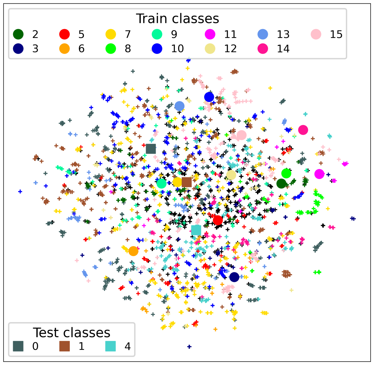
(a) Before training

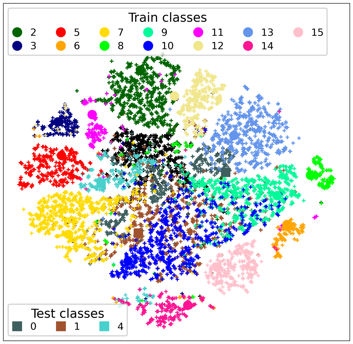
(b) After training

Figure 2: TSNE visualization on the embedding space, before and after training. Training organizes this space semantically and reduces the threadlike patterns representing close patches in the input image. Yet this is not completely solved for unseen classes during training.

References

- [1] Shaoqing Ren, Kaiming He, Ross Girshick, and Jian Sun. Faster r-cnn: Towards real-time object detection with region proposal networks. Advances in neural information processing systems, 28:91–99, 2015.
- [2] Joseph Redmon, Santosh Divvala, Ross Girshick, and Ali Farhadi. You only look once: Unified, real-time object detection. In Proceedings of the IEEE conference on computer vision and pattern recognition, pages 779–788, 2016.
- [3] Jake Snell, Kevin Swersky, and Richard Zemel. Prototypical networks for few-shot learning. In I. Guyon, U. V. Luxburg, S. Bengio, H. Wallach, R. Fergus, S. Vishwanathan, and R. Garnett, editors, Advances in Neural Information Processing Systems, volume 30. Curran Associates, Inc., 2017.
- [4] S Ravi H Larochelle. Optimization as a model for few-shot learning. In 5th International Conference on Learning Representations, ICLR 2017, Toulon, France, April 24-26, 2017, Conference Track Proceedings, 2017.
- [5] James Kirkpatrick, Razvan Pascanu, Neil Rabinowitz, Joel Veness, Guillaume Desjardins, Andrei A Rusu, Kieran Milan, John Quan, Tiago Ramalho, Agnieszka Grabska-Barwinska, et al. Overcoming catastrophic forgetting in neural networks. Proceedings of the national academy of sciences, 114(13):3521–3526, 2017.
- [6] Hao Chen, Yali Wang, Guoyou Wang, and Yu Qiao. Lstd: A low-shot transfer detector for object detection. In Proceedings of the AAAI Conference on Artificial Intelligence, volume 32, 2018.
- [7] Xin Wang, Thomas E. Huang, Trevor Darrell, Joseph E Gonzalez, and Fisher Yu. Frustratingly simple few-shot object detection. July 2020.
- [8] Xiaopeng Yan, Ziliang Chen, Anni Xu, Xiaoxi Wang, Xiaodan Liang, and Liang Lin. Meta r-cnn: Towards general solver for instance-level low-shot learning. In Proceedings of the IEEE/CVF International Conference on Computer Vision, pages 9577–9586, 2019.
- [9] Leonid Karlinsky, Joseph Shtok, Sivan Harary, Eli Schwartz, Amit Aides, Rogerio Feris, Raja Giryes, and Alex M Bronstein. Repmet: Representative-based metric learning for classification and few-shot object detection. In Proceedings of the IEEE/CVF Conference on Computer Vision and Pattern Recognition, pages 5197–5206, 2019.
- [10] Xiang Li, Jingyu Deng, and Yi Fang. Few-shot object detection on remote sensing images. IEEE Transactions on Geoscience and Remote Sensing, pages 1–14, 2021.
- [11] Zixuan Xiao, Jiahao Qi, Wei Xue, and P. Zhong. Few-shot object detection with self-adaptive attention network for remote sensing images. IEEE Journal of Selected Topics in Applied Earth Observations and Remote Sensing, 14:4854–4865, 2021.
- [12] Zhi Tian, Chunhua Shen, Hao Chen, and Tong He. Fcos: Fully convolutional one-stage object detection. In Proceedings of the IEEE/CVF International Conference on Computer Vision, pages 9627–9636, 2019.
- [13] Ross Girshick. Fast r-cnn. In Proceedings of the IEEE international conference on computer vision, pages 1440–1448, 2015.
- [14] Kaiming He, Xiangyu Zhang, Shaoqing Ren, and Jian Sun. Deep residual learning for image recognition. In Proceedings of the IEEE conference on computer vision and pattern recognition, pages 770–778, 2016.
- [15] Tsung-Yi Lin, Piotr Dollár, Ross Girshick, Kaiming He, Bharath Hariharan, and Serge Belongie. Feature pyramid networks for object detection. In Proceedings of the IEEE conference on computer vision and pattern recognition, pages 2117–2125, 2017.
- [16] Kaiming He, Georgia Gkioxari, Piotr Dollár, and Ross Girshick. Mask r-cnn. In Proceedings of the IEEE international conference on computer vision, pages 2961–2969, 2017.
- [17] Chelsea Finn, Pieter Abbeel, and Sergey Levine. Model-agnostic meta-learning for fast adaptation of deep networks. In International Conference on Machine Learning, pages 1126–1135. PMLR, 2017.
- [18] Jane Bromley, Isabelle Guyon, Yann LeCun, Eduard Säckinger, and Roopak Shah. Signature verification using a" siamese" time delay neural network. Advances in neural information processing systems, 6:737–744, 1993.
- [19] Flood Sung, Yongxin Yang, Li Zhang, Tao Xiang, Philip HS Torr, and Timothy M Hospedales. Learning to compare: Relation network for few-shot learning. In Proceedings of the IEEE conference on computer vision and pattern recognition, pages 1199–1208, 2018.
- [20] Oriol Vinyals, Charles Blundell, Timothy Lillicrap, koray kavukcuoglu, and Daan Wierstra. Matching networks for one shot learning. In D. Lee, M. Sugiyama, U. Luxburg, I. Guyon, and R. Garnett, editors, Advances in Neural Information Processing Systems, volume 29. Curran Associates, Inc., 2016.
- [21] Bingyi Kang, Zhuang Liu, Xin Wang, Fisher Yu, Jiashi Feng, and Trevor Darrell. Few-shot object detection via feature reweighting. In Proceedings of the IEEE/CVF International Conference on Computer Vision, pages 8420–8429, 2019.
- [22] Qi Fan, Wei Zhuo, Chi-Keung Tang, and Yu-Wing Tai. Few-shot object detection with attention-rpn and multi-relation detector. In CVPR, 2020.
- [23] Ting-I Hsieh, Yi-Chen Lo, Hwann-Tzong Chen, and Tyng-Luh Liu. One-shot object detection with co-attention and co-excitation. In H. Wallach, H. Larochelle, A. Beygelzimer, F. d'Alché-Buc, E. Fox, and R. Garnett, editors, Advances in Neural Information Processing Systems, volume 32. Curran Associates, Inc., 2019.
- [24] Junyoung Chung, Caglar Gulcehre, KyungHyun Cho, and Yoshua Bengio. Empirical evaluation of gated recurrent neural networks on sequence modeling, 2014.
- [25] Geonuk Kim, Hong-Gyu Jung, and Seong-Whan Lee. Few-shot object detection via knowledge transfer. In 2020 IEEE International Conference on Systems, Man, and Cybernetics (SMC), pages 3564–3569.
- [26] Jeffrey Pennington, Richard Socher, and Christopher D Manning. Glove: Global vectors for word representation. In Proceedings of the 2014 conference on empirical methods in natural language processing (EMNLP), pages 1532–1543.
- [27] Gong Cheng, Peicheng Zhou, and Junwei Han. Learning rotation-invariant convolutional neural networks for object detection in vhr optical remote sensing images. IEEE Transactions on Geoscience and Remote Sensing, 54(12):7405–7415, 2016.
- [28] Mathilde Caron, Piotr Bojanowski, Armand Joulin, and Matthijs Douze. Deep clustering for unsupervised learning of visual features. In Proceedings of the European Conference on Computer Vision (ECCV), pages 132–149, 2018.
- [29] Elad Hoffer and Nir Ailon. Deep metric learning using triplet network. In International workshop on similarity-based pattern recognition, pages 84–92. Springer, 2015.
- [30] Gui-Song Xia, Xiang Bai, Jian Ding, Zhen Zhu, Serge Belongie, Jiebo Luo, Mihai Datcu, Marcello Pelillo, and Liangpei Zhang. Dota: A large-scale dataset for object detection in aerial images. In Proceedings of the IEEE Conference on Computer Vision and Pattern Recognition, pages 3974–3983, 2018.
- [31] Mark Everingham, Luc Van Gool, Christopher KI Williams, John Winn, and Andrew Zisserman. The pascal visual object classes (voc) challenge. International journal of computer vision, 88(2):303–338, 2010.
- [32] Ting Chen, Simon Kornblith, Mohammad Norouzi, and Geoffrey Hinton. A simple framework for contrastive learning of visual representations. In International conference on machine learning, pages 1597–1607. PMLR, 2020.