2021 194 24 September

(Anti)nuclei in pp collisions at $\sqrt{s}=$ 13 TeV

ALICE Collaboration ALICE Collaboration

Understanding the production mechanism of light (anti)nuclei is one of the key challenges of nuclear physics and has important consequences for astrophysics, since it provides an input for indirect dark-matter searches in space. In this paper, the latest results about the production of light (anti)nuclei in pp collisions at $\sqrt{s}$ $=13$ TeV are presented, focusing on the comparison with the predictions of coalescence and thermal models. For the first time, the coalescence parameters $B_{2}$ for deuterons and $B_{3}$ for helions are compared with parameter-free theoretical predictions that are directly constrained by the femtoscopic measurement of the source radius in the same event class. A fair description of the data with a Gaussian wave function is observed for both deuteron and helion, supporting the coalescence mechanism for the production of light (anti)nuclei in pp collisions. This method paves the way for future investigations of the internal structure of more complex nuclear clusters, including the hypertriton.

1 Introduction

In high-energy hadronic collisions at the LHC, the production of light (anti)nuclei and more complex multi-baryon bound states, such as (anti)hypertriton [1], is observed. An unexpectedly large yield of light nuclei was observed for the first time in proton-nucleus collisions at the CERN PS accelerator [2]. Twenty-five years later, the study of nuclear production was carried out at Brookhaven AGS and at CERN SPS, with the beginning of the program of relativistic nuclear collisions [3]. Extensive studies of the production of light (anti)nuclei were later performed at the Relativistic Heavy-Ion Collider (RHIC) [4, 5, 6, 7], including the first observation of an antihypernucleus [8] and of anti(alpha) [9]. In this paper, the focus will be on results obtained at LHC. The production yields of light (anti)nuclei have been measured as a function of transverse momentum ($p_{\rm T}$) and charged-particle multiplicity in different collision systems and at different center-of-mass energies by ALICE [10, 11, 12, 13, 14, 15, 16, 17]. One of the most interesting observations obtained from such a large variety of experimental data is that the production of light (anti)nuclei seems to depend solely on the charged-particle multiplicity (hereinafter denoted multiplicity). This observation manifests itself in the continuous evolution of the deuteron-to-proton (d/p) and ³He-to-proton (³He/p) ratios with the event multiplicity across different collision systems and energies [16, 17]. The results presented in this paper complement the existing picture, providing measurements in yet unexplored multiplicity regions.

These measurements have an important astrophysical value as they provide input for the background estimates in indirect dark matter searches in space. Indeed, only small systems like pp collisions are relevant for such searches because the interstellar medium consists mostly of hydrogen (protons) and helium (alpha particles). In this context, the observation of a significant antimatter excess with respect to the expected background of antimatter produced in ordinary cosmic ray pp or p–alpha interactions would represent a signal for dark matter annihilation in the galactic halo or for the existence of antimatter islands in our universe [18, 19, 20, 21].

The theoretical description of the production mechanism of (anti)nuclei is still an open problem and under intense debate in the scientific community. Two phenomenological models are typically used to describe the production of multi-baryon bound states: the statistical hadronisation model (SHM) [22, 23, 24, 25, 26, 27, 28] and the coalescence model [29, 30, 31, 32, 33, 34]. In the former, light nuclei are assumed to be emitted by a source in local thermal and hadrochemical equilibrium and their abundances are fixed at chemical freeze-out. The version of this model using the grand-canonical ensemble reproduces the light-flavoured hadron yields measured in central nucleus–nucleus collisions, including those of (anti)nuclei and (anti)hypernuclei [22]. In pp and p–Pb collisions, the production of light nuclei can be described using a different implementation of this model based on the canonical ensemble, where exact conservation of the electric charge, strangeness, and baryon quantum numbers is applied within a pre-defined correlation volume [25, 28]. In the coalescence model, light nuclei are assumed to be formed by the coalescence of protons and neutrons which are close in phase space at kinetic freeze-out [30]. In the most simple version of this model, nucleons are treated as point-like particles and only correlations in momentum space are considered, i.e. the bound state is assumed to be formed if the difference between the momenta of nucleons is smaller than a given threshold $p_{0}$, a free parameter of the model which is typically of the order of 100 MeV$/\textit{c}$. This simple version of the coalescence model can approximately reproduce deuteron production data in low-multiplicity collisions and was recently used to describe the jet-associated deuteron $p_{\rm T}$-differential yields in pp collisions at $\sqrt{s}=$13 TeV [35]. In recent developments [31, 36], the quantum-mechanical properties of nucleons and nuclei are taken into account and the coalescence probability is calculated from the overlap between the source function of the emitted protons and neutrons, which are mapped on the Wigner density of the nucleus. This state-of-the-art coalescence model describes the d/p and ³He/p ratios measured in different collision systems as a function of multiplicity [33]. On the contrary, the simple coalescence approach provides a description of $p_{\rm T}$ spectra of light (anti)nuclei measured in high-energy hadronic collisions only in the low-multiplicity regime [15].

In this paper, the measurement of the production yields of light (anti)nuclei in pp collisions at $\sqrt{s}=$13 TeV are presented. In particular, part of the results is obtained from data collected with a high-multiplicity trigger (see Sec. 2), accessing a multiplicity typically obtained in p–Pb and peripheral Pb–Pb collisions. For the first time, the yields of (anti)nuclei are measured in a multiplicity region in which high-precision femtostopic measurements of the source size [37] are available. This allows for a parameter-free comparison of the coalescence measurements with theoretical calculations, showing the potential of this technique to set constraints on the wave function of (anti)nuclei.

2 Detector and data sample

A detailed description of the ALICE apparatus and its performance can be found in Refs. [38] and [39]. The trajectories of charged particles are reconstructed in the ALICE central barrel with the Inner Tracking System (ITS) [40] and the Time Projection Chamber (TPC) [41]. The ITS consists of six cylindrical layers of silicon detectors and the two innermost layers form the Silicon Pixel Detector (SPD). The ITS is used for the reconstruction of primary and secondary vertices and of charged-particle trajectories. The TPC is used for track reconstruction, charged-particle momentum measurement and for charged-particle identification via the measurement of their specific energy loss ($\textrm{d}E/\textrm{d}x$) in the TPC gas [39]. Particle identification at high momentum is complemented by the time-of-flight measurement provided by the TOF detector [42]. The aforementioned detectors are located inside a large solenoid magnet, which provides a homogeneous magnetic field of 0.5 T parallel to the beam line, and cover the pseudorapidity interval $|\eta|<0.9$. Collision events are triggered by two plastic scintillator arrays, V0C and V0A [43], located along the beam axis of the interaction point, covering the pseudorapidity regions $-$3.7 $<\eta<$ $-$1.7 and 2.8 $<\eta<$ 5.1, respectively. The signals from V0A and V0C are summed to form the V0M signal, which is used to define event classes to which the measured multiplicity is associated [44]. Moreover, the timing information of the V0 detectors is used for the offline rejection of events triggered by interactions of the beam with the residual gas in the LHC vacuum pipe.

The results presented in this paper are obtained from data collected in 2016, 2017 and 2018, both with minimum bias (MB) and high multiplicity (HM) triggers. For the minimum-bias event trigger, coincident signals in both V0 scintillators are required to be synchronous with the beam crossing time defined by the LHC clock. Events with high charged-particle multiplicities are triggered on by additionally requiring the total signal amplitude measured in the V0 detector to exceed a threshold. At the analysis level, the 0–0.1% percentile of inelastic events with the highest V0 multiplicity (V0M) is selected to define the high-multiplicity event class. Events with multiple vertices identified with the SPD are tagged as pile-up in the same bunch crossing (in-bunch pile-up) and removed from the analysis [39]. Assuming that all the in-buch pile-up is in the 0–0.01% percentile of inelastic events, which is the worst-case scenario, only 3% of the selected events (in the 0–0.01% percentile) would be pile-up events. Therefore, the effect of in-bunch pile-up on the production spectra is negligible. Pile-up in different bunch crossings, instead, is rejected by requiring track hits in the SPD and its contribution is negligible. The data sample consists of approximately 2.6 billion MB events and 650 million HM events.

For the measurements of (anti)protons and (anti)deuterons, the high-multiplicity data sample is divided into three multiplicity classes: HM I, HM II and HM III. The multiplicity classes are determined from the sum of the signal amplitudes measured by the V0 detectors and defined in terms of the percentiles of the INEL $>$ 0 pp cross section, where an INEL $>$ 0 event is a collision with at least a charged particle in the pseudorapidity region $|\eta|<1$ [45]. For this purpose, charged particles are measured with SPD tracklets, obtained from a pair of hits in the first and second layer of the SPD, respectively. In the case of (anti)triton (${}^{3}\mathrm{H}$) and (anti)helion (${}^{3}\mathrm{He}$), due to their lower production rate, it is not possible to divide the HM sample into smaller classes, but for (anti)helion the MB sample is divided into two multiplicity classes, MB I and MB II, defined from the percentiles of the INEL $>$ 0 pp cross section. The average charged particle multiplicity $\langle\mathrm{d}N_{\mathrm{ch}}/\mathrm{d}\eta\rangle$ for all the multiplicity classes will be reported in Tab. 2. It is defined as the number of primary charged particles produced in the pseudorapidity interval $|\eta|<0.5$. A detailed description of the $\langle\mathrm{d}N_{\mathrm{ch}}/\mathrm{d}\eta\rangle$ estimation can be found in Ref. [46].

3 Data analysis

3.1 Track selection

(Anti)nuclei candidates are selected from the charged-particle tracks reconstructed in the ITS and TPC in the pseudorapidity interval $|\eta|<0.8$. The criteria used for track selection are the same as reported in Ref. [17]. Particle identification is performed using the $\textrm{d}E/\textrm{d}x$ measured by the TPC and the time-of-flight measured by the TOF. For the TPC analysis, the signal is obtained from the $n\sigma_{\mathrm{TPC}}$ distribution, where $n\sigma_{\mathrm{TPC}}$ is the difference between the measured and expected signals for a given particle hypothesis, divided by the resolution. For the TOF analysis, the yield in each $p_{\rm T}$ interval is extracted from the distribution of the TOF squared-mass, defined as $m^{2}=p^{2}\left(t_{\mathrm{TOF}}^{2}/L^{2}-1/c^{2}\right)$, where $t_{\mathrm{TOF}}$ is the measured time-of-flight, $L$ is the length of the track and $p$ is the momentum of the particle. Similarly to the TPC case, one defines $n\sigma_{\mathrm{TOF}}$ as the difference between the measured and expected time of flight for a given particle hypothesis, divided by the resolution. For the TOF analysis, a pre-selection based on the measured TPC $\textrm{d}E/\textrm{d}x$ ($|n\sigma_{\mathrm{TPC}}|<3$) is performed to reduce the background originating from other particle species. More details about particle identification with TPC and with TOF can be found in Ref. [17].

The (anti)deuteron yield is extracted from the TPC signal for $p_{\mathrm{T}}<$ 1 GeV$/$c, while at higher $p_{\rm T}$ the yield is extracted from the TOF after the pre-selection using the TPC signal. For (anti)protons, the TOF is used for the entire $p_{\rm T}$ range. (Anti)tritons are identified through the TPC signal and after a pre-selection with TOF ($|n\sigma_{\mathrm{TOF}}|<3$) for $p_{\mathrm{T}}<$ 2 GeV$/$c. The (anti)helion identification is based only on the TPC $\textrm{d}E/\textrm{d}x$, which provides a good separation of its signal from that of other particle species. This is due to the charge $\mathrm{Z}=2$ of this nucleus.

3.2 Efficiency and acceptance correction

The estimation of reconstruction efficiencies of both nuclei and antinuclei, as well as those of the contamination to the raw $p_{\rm T}$ spectra of nuclei from spallation and of the signal loss due to event selection, requires Monte Carlo (MC) simulations. Simulated pp collision events, generated using Pythia 8 [47] (Monash 2013 tune [48]), are enriched by an injected sample of (anti-)nuclei generated with a flat $p_{\rm T}$ distribution in the transverse-momentum range $0<p_{\mathrm{T}}<10\ \mathrm{GeV}/\textit{c}$ and a flat rapidity distribution in the range $|y|<1$. The interactions of the generated particles with the experimental apparatus are modeled by GEANT4 [49]. The detector conditions during the data taking are reproduced in the simulations.

The raw $p_{\rm T}$ spectra of (anti)nuclei are corrected for the reconstruction efficiency and acceptance, defined as

$$\epsilon(p_{\mathrm{T}})=\frac{N_{\mathrm{rec}}(|\eta|<0.8,|y|<0.5,p^{\mathrm{rec}}_{\mathrm{T}})}{N_{\mathrm{gen}}(|y|<0.5,p_{\mathrm{T}})},$$ (1)

where $N_{\mathrm{rec}}$ and $N_{\mathrm{gen}}$ are the number of reconstructed and generated (anti)nuclei, respectively. The same criteria for the track selection and particle identification used in the real data analysis are applied to reconstructed tracks in the simulation. Considering that (anti)nuclei are injected with a flat $p_{\rm T}$ distribution into the simulated events, their input distributions are reshaped using $p_{\rm T}$-dependent weights to match the real shape observed in data. The latter is parameterised using a Lévy-Tsallis function whose parameters are determined using an iterative procedure: they are initialized using the values taken from Ref. [17], the corrected spectrum is then fitted with the same function and a new set of parameters is determined and used for the next iteration. The parameters are found to converge after two iterations, with differences from the previous one of less than one per mille. Protons are abundantly produced by Pythia 8 and their spectral shape is consistent with the one obtained in real data. For this reason, (anti)protons are not injected additionally into the simulation and their shape is not modified.

3.3 Fraction of primary nuclei

Secondary nuclei are produced in the interaction of particles with the detector material. To obtain the yields of primary nuclei produced in a collision, the number of secondaries must be subtracted from the measured yield. Since the production of secondary antinuclei is extremely rare, this correction is applied only to nuclei and not to antinuclei. For (anti)protons, instead, also a contribution from weak decays of heavier unstable particles (for example $\Lambda$ hyperons) is present and cannot be neglected. The fraction of primary nuclei is evaluated using different techniques according to the analysis.

For deuterons and (anti)protons, the primary fraction is obtained by fitting the distribution of the measured distance of closest approach to the primary vertex in the transverse plane (DCA_xy). For the fit, templates obtained from MC are used, as described in Ref. [10]. The DCA_xy distribution of anti-deuterons is used as a template for primary deuterons considering the negligible feed-down from weak decays of hypertriton. The production of secondary deuterons is more relevant at low $p_{\mathrm{T}}$ (at $p_{\mathrm{T}}=$ 0.7 GeV$/$c the fraction of secondary deuterons is $\sim$ 40%), decreases exponentially with the transverse momentum ($<$ 5% for $p_{\mathrm{T}}=$ 1.4 GeV$/$c) and becomes negligible for $p_{\mathrm{T}}>$ 1.6 GeV$/$c. For the (anti)proton analysis, all the templates are taken from MC. In this case, also a template for weak decay is used. The fraction of secondary protons from material is maximum at low transverse momentum ($\sim$5% for $p_{\mathrm{T}}=$ 0.4 GeV$/$c) and decreases exponentially, becoming negligible for $p_{\mathrm{T}}>$ 1 GeV$/$c. Also, the fraction of secondary (anti)protons from weak decays is maximum at low transverse momentum ($\sim$30% for $p_{\mathrm{T}}=$ 0.4 GeV$/$c) and decreases exponentially ($\sim$10% for $p_{\mathrm{T}}=$ 5 GeV$/$c).

For helion and triton, the primary fraction is obtained by fitting the DCA_xy distribution with two Gaussian functions with different widths, one for the primary and one for the secondary nuclei, respectively. The spallation background is also fitted using a parabola and a constant function to estimate the systematic uncertainties. For the latter, variations of the binning and fit range are also considered. A smooth function can be used in this case, considering that the peak in the DCA_xy distribution of secondary nuclei, which typically appears close to zero and is caused by the wrong association of one SPD cluster to the track during reconstruction, is negligible for $p_{\mathrm{T}}>1.5$ GeV$/c$. The fraction of secondary helions and tritons, for both MB and HM pp collisions, are found to be about 15$\%$ in the $p_{\rm T}$ interval $1.5<p_{\mathrm{T}}<2$ GeV$/$c, about 3$\%$ in the $p_{\rm T}$ interval $2<p_{\mathrm{T}}<2.5$ GeV$/$c and negligible for higher $p_{\rm T}$. For tritons and helions, only antinuclei are used for $p_{\mathrm{T}}<1.5$ GeV$/$c, where the secondary fraction for nuclei becomes large and it is difficult to constrain the value of the correction.

3.4 Systematic uncertainties

A summary of the systematic uncertainties for all the measurements is reported in Tab. 1. Values are provided for low (1.5 GeV$/c$) and high (4 GeV$/c$) transverse momentum. Where the systematic uncertainty differs between matter and antimatter, the latter is reported within brackets. The first source of systematic uncertainty is related to track selection. This source takes into account the imprecision in the description of the detector response in the MC simulation. The uncertainties are evaluated by varying the relevant selection criteria, as done in Ref. [11]. It is worth mentioning that at low $p_{\rm T}$ uncertainties are generally larger for matter than for antimatter, due to the increasing number of secondary nuclei selected when loosing the selection on the DCA. It is one of the main sources. The second source is related to signal extraction. It is evaluated by changing the fit function used to evaluate the raw yield or, when the direct count is used, by varying the interval in which the count is performed (see Ref. [11] and Ref. [17] for further details). Its value increases with transverse momentum. The effect of the incomplete knowledge of the material budget of the detector is evaluated by comparing different MC simulations in which the material budget is varied by $\pm$4.5%. This value corresponds to the uncertainty on the determination of the material budget by measuring photon conversions [39]. Similarly, the limited precision in the measurements of inelastic cross sections of (anti)nuclei with matter is a source of systematic uncertainty. It is evaluated by comparing experimental measurements of the inelastic cross section with the values implemented in GEANT4, following the same approach used in Ref. [50]. For antihelion, the difference between the momentum-dependent inelastic cross sections implemented in GEANT3 [51] and GEANT4 is also considered. This contribution is maximum (3$\%$) for $p_{\rm T}<1.5$ GeV/$c$ and decreases to a negligible level going to higher $p_{\rm T}$. Finally, the last sources of systematic uncertainty are related to the matching of the tracks between ITS and TPC and between TPC and TOF. They are evaluated from the difference between the ITS–TPC (TPC–TOF) matching in data and MC.

Table 1: Summary of the main contributions to the systematic uncertainties for all the particle species under study at $p_{\mathrm{T}}=1.5$ GeV/$c$ and at $p_{\mathrm{T}}=4$ GeV/$c$. Values in brackets refer to antiparticles. If they are not present, the systematic uncertainty is the same for particles and antiparticles. A dash symbol is used where the uncertainty from the corresponding source is not applicable. More details about the sources of the uncertainties can be found in the text.

Source	$p_{\mathrm{T}}=1.5$ GeV$/c$				$p_{\mathrm{T}}=4$ GeV$/c$
	p ($\overline{\mathrm{p}}$)	d ($\overline{\mathrm{d}}$)	3He (${}^{3}\overline{\mathrm{He}}$)	3H (${}^{3}\overline{\mathrm{H}}$)	p ($\overline{\mathrm{p}}$)	d ($\overline{\mathrm{d}}$)	3He (${}^{3}\overline{\mathrm{He}}$)
Track selection	3%	1%	14% (10%)	14% (10%)	3%	2%	10% (7%)
Signal extraction	<1%	3%	13% (<1%)	<1%	5%	2%	<1%
Material budget	1%	1%	2%	2%	1%	<1%	2%
Hadronic interaction	1% (2%)	2% (6%)	1% (2%)	9% (6%)	1% (2%)	2% (6%)	1% (1%)
ITS–TPC matching	2%	2%	2%	2%	2%	2%	2%
TPC–TOF matching	3%	2%	$-$	3%	3%	2%	$-$
Total	6% (7%)	4% (7%)	22% (11%)	20% (17%)	7% (8%)	4% (7%)	8%

4 Results and discussion

The production spectra for all the species under study are shown in Fig. 1. The multiplicity classes used for this measurement are reported in Tab 2, together with the corresponding $p_{\rm T}$-integrated yields. (Anti)protons, (anti)deuterons and (anti)helions are fitted with a Lévy-Tsallis function [52], which is used to extrapolate the yields in the unmeasured $p_{\rm T}$ region. For (anti)triton, the fit parameters (except for the mass and the normalisation) are fixed to those of (anti)helion, due to the few data points available. The extrapolation amounts to about 20% of the total $p_{\rm T}$-integrated yield for (anti)protons and (anti)deuterons, about 30% for (anti)helions, and about 50% for (anti)tritons. Alternative fit functions such as a simple exponential depending on $m_{\rm T}$, a Boltzmann function or a Blast-wave function [53, 54, 55], are used to evaluate the systematic uncertainty on the $p_{\rm T}$-integrated yield as done in Ref. [17, 15, 16]. This uncertainty varies between 0.5% and 3% for protons, deuterons and helions in the HM analysis. For tritons it is around 8% due to the narrower $p_{\rm T}$ coverage. In the MB analysis, it is around 8% (14%) for helions (tritons).

Table 2: Multiplicity classes for the different measurements, with the corresponding multiplicity $\langle$d$N_{\mathrm{ch}}/$d$\eta\rangle_{|\eta_{\mathrm{lab}}|<0.5}$, and $p_{\rm T}$-integrated yields d$N/$d$y$ for the different species (average for particle and antiparticle). For $\langle$d$N_{\mathrm{ch}}/$d$\eta\rangle_{|\eta_{\mathrm{lab}}|<0.5}$, only the systematic uncertainty is reported, because the statistical one is negligible. For d$N/$d$y$, the first uncertainty is statistical and the second is systematic.

Multiplicity	$\langle$d$N_{\mathrm{ch}}/$d$\eta\rangle_{|\eta_{\mathrm{lab}}|<0.5}$	d$N/$d$y$
		p	d	3He	3H
HM	31.5 $\pm$ 0.3	0.80 $\pm$ 0.01 $\pm$ 0.05		(23.3 $\pm$ 1 $\pm$ 3) $\times 10^{-7}$	(25 $\pm$ 2 $\pm$ 4) $\times 10^{-7}$
HM I	35.8 $\pm$ 0.5	0.91 $\pm$ 0.01 $\pm$ 0.05	(22.1 $\pm$ 0.1 $\pm$ 1.4) $\times 10^{-4}$
HM II	32.2 $\pm$ 0.4	0.83 $\pm$ 0.01 $\pm$ 0.05	(19.8 $\pm$ 0.1 $\pm$ 1.3) $\times 10^{-4}$
HM III	30.1 $\pm$ 0.4	0.77 $\pm$ 0.01 $\pm$ 0.04	(18.4 $\pm$ 0.1 $\pm$ 1.1) $\times 10^{-4}$
MB	6.9 $\pm$ 0.1			(2.4 $\pm$ 0.3 $\pm$ 0.4) $\times 10^{-7}$	(1.7 $\pm$ 0.3 $\pm$ 0.4) $\times 10^{-7}$
MB I	18.7 $\pm$ 0.3			(11 $\pm$ 2 $\pm$ 2) $\times 10^{-7}$
MB II	6.0 $\pm$ 0.2			(1.5 $\pm$ 0.2 $\pm$ 0.3) $\times 10^{-7}$

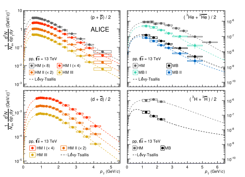
Figure 1: Transverse-momentum spectra of (anti)protons, (anti)deuterons, (anti)helion, and (anti)triton, measured in HM and MB pp collisions at $\sqrt{s}~{}=~{}$13 TeV at midrapidity ($|y|<0.5)$. The results are shown in the multiplicity classes reported in Tab. 2. Vertical bars and boxes represent statistical and systematic uncertainties, respectively. The dashed lines are individual fits with a Lévy-Tsallis function.

4.1 Coalescence parameter as a function of transverse momentum

In the coalescence model, the production probability of a nucleus with mass number $A$ is proportional to the coalescence parameter $B_{A}$, defined as

$$B_{A}\left(p_{\mathrm{T}}^{\mathrm{p}}\right)=\frac{1}{2\pi p_{\mathrm{T}}^{\mathrm{A}}}\frac{\mathrm{d}^{2}N_{\mathrm{A}}}{\mathrm{d}y\mathrm{d}p^{\mathrm{A}}_{\mathrm{T}}}\;\bigg{/}\left(\frac{1}{2\pi p_{\mathrm{T}}^{\mathrm{p}}}\frac{\mathrm{d}^{2}N_{\mathrm{p}}}{\mathrm{d}y\mathrm{d}p_{\rm T}^{\mathrm{p}}}\right)^{A},$$ (2)

where the labels $\mathrm{p}$ and $\mathrm{A}$ refer to protons and the (anti)nucleus with mass-number $A$, respectively. The invariant spectra of the (anti)protons are evaluated at the transverse momentum of the (anti)nucleus, divided by the mass-number $A$. For (anti)deuterons, for example, $B_{A}=B_{2}$ and $p_{\mathrm{T}}^{\mathrm{p}}=p_{\mathrm{T}}^{\mathrm{A}}/A=p_{\mathrm{T}}^{\mathrm{d}}/2$.

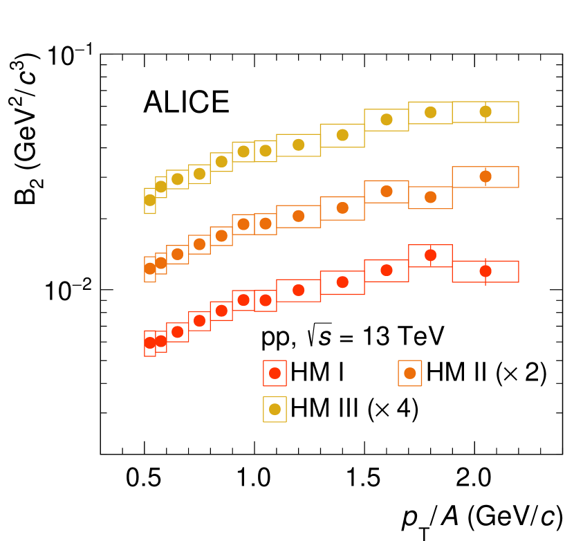
(a) (Anti)deuterons

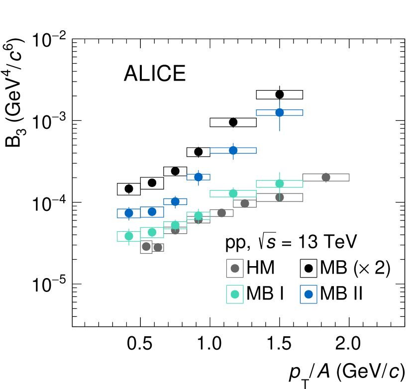
(b) (Anti)helions

Figure 2: Coalescence parameters $B_{2}$ (a) and $B_{3}$ (b) as a function of $p_{\mathrm{T}}/A$ for the multiplicity classes reported in Tab. 2. Vertical bars and boxes represent statistical and systematic uncertainties, respectively.

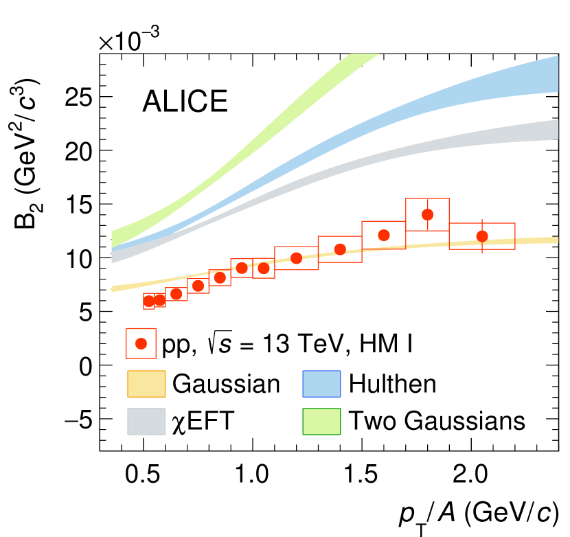
(a) (Anti)deuterons

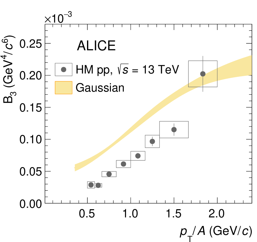
(b) (Anti)helions

Figure 3: Comparison between measurements and theoretical predictions for the coalescence parameters $B_{2}$ for (anti)deuterons (a) and $B_{3}$ for (anti)helions (b) as a function of $p_{\mathrm{T}}/A$. Vertical bars and boxes represent statistical and systematic uncertainties, respectively. Theoretical predictions are obtained using different wave functions to describe nuclei: Gaussian (yellow), Hulthen (blue), $\chi\text{EFT}$ (gray) and two Gaussians (green).

The coalescence parameters for (anti)deuterons ($B_{2}$) and for (anti)helions ($B_{3}$) are shown in Fig. 2 as a function of $p_{\rm T}/A$ for different multiplicity classes. Some of the measurements are scaled for better visibility (see the legend), but for $B_{2}$ the three curves are consistent with each other. A clear increase of both $B_{2}$ and $B_{3}$ with increasing $p_{\rm T}/A$ is observed. Previous measurements of $B_{2}$ in pp [17, 11] and p–Pb [15] collisions indicated an almost flat trend with $p_{\rm T}/A$. However, in Ref. [17] and in Ref. [11] it was shown that even though $B_{2}$ evaluated in multiplicity classes was flat, $B_{2}$ evaluated in the multiplicity-integrated sample showed a rise with $p_{\rm T}/A$. The trend shown in Ref. [11] is a consequence of the mathematical definition of $B_{2}$ and of the hardening of the proton spectra. Given the narrow multiplicity intervals used in the present measurement, the significant rise of the coalescence parameters with $p_{\rm T}/A$ cannot be attributed to effects originating from a different hardening of the (anti)proton and (anti)nuclei spectra within these multiplicity intervals [11].

The measurement of the coalescence parameter as a function of transverse momentum is compared with predictions from the coalescence model, using different nuclei wave functions [56] and the precise measurement of the source radii for the same data set [37]. In the case of (anti)deuterons, the following wave functions are used: single and double Gaussian [34], Hulthen [32], and a function obtained from chiral Effective Field Theory ($\chi\text{EFT}$) of order N4LO with a cutoff at 500 MeV [57]. For (anti)helion, only calculations using a Gaussian wave function are currently available, because the general recipe used for $B_{2}$ cannot be extended to $B_{3}$ but new calculations ab initio are needed. These wave functions and more details about the adopted theoretical models can be found in Appendix A. In the coalescence model, the coalescence parameter depends on the radial extension of the particle emitting source [56]. The source radius is measured in HM pp collisions at $\sqrt{s}=$ 13 TeV by ALICE using p–p and p–$\Lambda$ correlations as a function of the mean transverse mass $\langle m_{\rm T}\rangle$ of the pair  [37]. In Ref. [37] two different measurements of the source radius are reported, $r_{\mathrm{effective}}$ and $r_{\mathrm{core}}$, respectively. The difference between the two is that $r_{\mathrm{core}}$ takes into account the contributions coming from the strong decay of resonances by subtracting them. It is shown that $r_{\mathrm{core}}$ is universal, since it could describe simultaneously p–p and p–$\Lambda$ correlations. In this analysis, $r_{\mathrm{core}}$ is used. The difference between $r_{\mathrm{core}}$ and $r_{\mathrm{effective}}$ is small: $B_{2}$ is on average 7% smaller using $r_{\mathrm{effective}}$, while $B_{3}$ is on average 20% smaller, due to the stronger dependence on the system size for $A>$2 (see Eq. 9). For $B_{2}$, only the HM I class is considered, because the $B_{2}$ values in the three multiplicity classes are compatible.

The data in Ref. [37] are parameterised as $r_{\rm source}(\langle m_{\rm T}\rangle)=c_{0}+\mathrm{exp}(c_{1}+c_{2}\langle m_{\rm T}\rangle)$, with $c_{i}$ free parameters, to map the transverse-mass to the source radius. The value of $p_{\rm T}$ corresponding to $m_{\mathrm{T}}$ is taken from $m_{\rm T}=\sqrt{m^{2}_{\rm p}+(p_{\mathrm{T}}/A)^{2}}$, where $m_{\rm p}$ is the proton mass. The radius of the deuteron and ³He are taken from Ref. [58]. The coalescence predictions are shown in comparison with the data in Fig. 3. Bands represent the uncertainty propagated from the measurement of the source radius. In the case of $B_{2}$, the Gaussian wave function provides the best description of the data, even though the Hulthen wave function is favoured by low-energy scattering experiments [59]. The other wave functions are significantly larger than the measurement. For the $B_{3}$, the coalescence predictions using a Gaussian wave function of helion are above the data by almost a factor of 2 except for the last $p_{\rm T}$ interval, which is consistent with the measured $B_{3}$ within the uncertainties. In the future, a systematic investigation of the coalescence parameter $B_{3}$ using different wave functions, in the context of the coalescence model, will gauge the potential of coalescence measurements to further constrain the wave function of helion. This technique can be used in a more general context to obtain information on the internal wave function of more complex (hyper)nuclei, such as alpha (⁴He) and hypertriton.

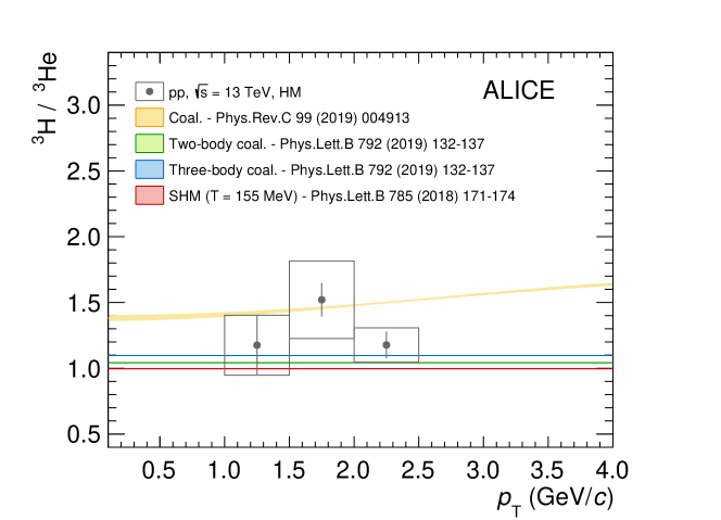
Figure 4: Ratio between the $p_{\rm T}$ spectra of triton and helion for the HM data sample. Vertical bars and boxes represent statistical and systematic uncertainties, respectively. The measurements are compared with the prediction of thermal (red) and coalescence models from Ref. [36] (yellow) and Ref. [33] (green and blue).

4.2 Ratio between triton and helion yields

The statistical hadronisation and coalescence models predict different yields of nuclei with similar masses but different radii. To test the production model, the ratio of triton and helion is measured as a function of $p_{\rm T}$ for HM pp collisions (Fig. 4) and compared with the model predictions. Two different versions of coalescence are considered, based on Ref. [33] and Ref. [36], respectively. The main difference between the two models concerns the source size $R$: while in Ref. [33] the value of $R$ is constrained from the parameters of a thermal fit, in Ref. [36] $R$ is an independent variable, for which the aforementioned $p_{\rm T}$ dependence has been taken into account. In the former approach, $R$ is about a factor of 2 larger than in the latter, determining very different predictions. The coalescence model predicts a slightly larger yield of triton as compared to helion due to its smaller nuclear radius. In the statistical hadronisation model, the yield ratio between these two nuclei is given by $\exp(-\Delta m/T_{\rm chem})$, where $\Delta m$ is the mass difference between triton and helion, taken from Ref. [60], and $T_{\rm chem}$ the chemical freeze-out temperature. For the latter, $T_{\rm chem}=155$ MeV is used, as done in the canonical statistical model [61]. Given the small mass difference, the statistical hadronisation model predicts a ratio which is very close to unity. The precision of the present data prevents distinguishing between the models. The ³H/³He ratio will be measured with higher precision in Run 3 [62] of the LHC. Indeed, the new ITS, which is characterised by a low material budget, will reduce the systematic uncertainty related to track reconstruction [63]. Moreover, with a better description of the nuclear absorption cross section, it will be possible to reduce the corresponding systematic uncertainties.

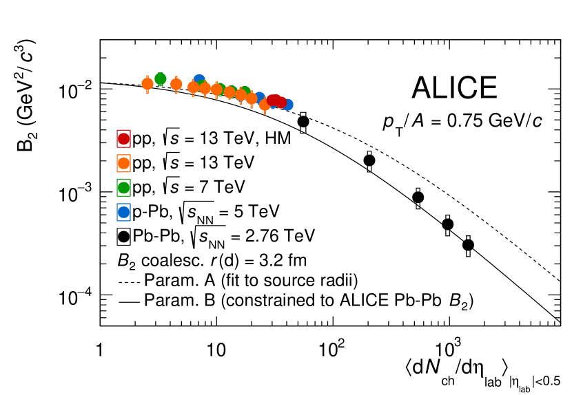
(a) (Anti)deuterons

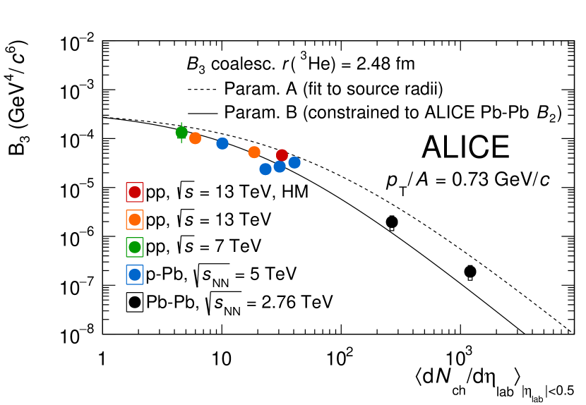
(b) (Anti)helions

Figure 5: (a): $B_{2}$ at $p_{\mathrm{T}}/A=$ 0.75 GeV/c as a function of multiplicity in HM pp collisions at $\sqrt{s}~{}=~{}13$ TeV, in MB pp collisions at $\sqrt{s}~{}=~{}13$ TeV [17] and at $\sqrt{s}~{}=~{}7$ TeV [11], in p–Pb collisions at $\sqrt{s_{\mathrm{NN}}}~{}=~{}5.02$ TeV [15], and in Pb–Pb collisions at $\sqrt{s_{\mathrm{NN}}}~{}=~{}2.76$ TeV [10]. (b): $B_{3}$ at $p_{\mathrm{T}}/A=$ 0.73 GeV$/$c as a function of multiplicity in HM pp collisions at $\sqrt{s}~{}=~{}13$ TeV, in MB pp collisions at $\sqrt{s}~{}=~{}13$ TeV, in p–Pb collisions at $\sqrt{s_{\mathrm{NN}}}~{}=~{}5.02$ TeV [15], and in Pb–Pb collisions at $\sqrt{s_{\mathrm{NN}}}~{}=~{}2.76$ TeV [10]. Vertical bars and boxes represent statistical and systematic uncertainties, respectively. The two lines are theoretical predictions based on two different parameterisations of the source radius.

4.3 Coalescence parameter as a function of multiplicity

The evolution of $B_{A}$ with multiplicity $\langle\mathrm{d}N_{\mathrm{ch}}/\mathrm{d}\eta\rangle$ provides an insight on the dependence of the production mechanisms of light (anti)nuclei. Fig. 5(a) shows $B_{2}$ as a function of $\langle\mathrm{d}N_{\mathrm{ch}}/\mathrm{d}\eta\rangle$ for different collision systems and energies at $p_{\rm T}~{}=~{}0.75$ GeV$/c$ and $B_{3}$ at $p_{\rm T}~{}=~{}0.73$ GeV$/c$. The measurements are compared with the theoretical predictions from Ref. [58], using $r(\mathrm{d})=3.2$ fm and $r(^{3}\mathrm{He})=2.48$ fm as deuteron and helion radii, respectively. Two different parameterisations (named A and B in the following) of the system radius as a function of multiplicity are used. Parameterisation A is based on a fit to the ALICE measurements of system radii $R$ from femtoscopic measurement as a function of multiplicity [64]. In parameterisation B, the relation between the system radius and the multiplicity is fixed to reproduce the $B_{2}$ of deuterons in Pb–Pb collisions at $\sqrt{s_{\mathrm{NN}}}=2.76$ TeV in the centrality class 0–10% (see Ref. [58] for more details). The $B_{2}$ measurement in HM pp collisions agrees with observations in p–Pb collisions at $\sqrt{s_{\mathrm{NN}}}=$ 5 TeV [15] at similar multiplicity and confirms the trend observed in all the previous measurements. This measurement further strengthen the idea of a production mechanism that depends only on the multiplicity and not on the collision system nor the centre-of-mass energy. Similarly, Fig. 5(b) shows the evolution of $B_{3}$ as a function of multiplicity. The measurements are compared with the theoretical prediction from Ref. [58], using the same two paremeterisations as for $B_{2}$. Also in this case, the coalescence model qualitatively describes the trend but fails in accurately describing the measurements in the whole multiplicity range. For both $B_{2}$ and $B_{3}$, one reason could be that multiplicity is not a perfect proxy for the system size, because for each multiplicity the source radius depends also on the transverse momentum of the particle of interest, as shown in Fig. 2. In the future, it is important to have more measurements of the source radius as a function of $m_{\rm T}$ for the different multiplicity classes in order to test the agreement between the models and the $B_{A}$ measurement over the whole multiplicity range.

4.4 Ratio between integrated yields of nuclei and protons as a function of multiplicity

The measurements of the ratios between the $p_{\rm T}$-integrated yields of nuclei and protons as a function of multiplicity are shown. Figure 6 shows the measurement for different collision systems and energies for deuterons (d$/$p) and helions (³He$/$p), on the left and right panels, respectively. The new measurements complement the existing picture and are consistent with the global trend obtained from previous measurements  [10, 11, 12, 13, 14, 15, 16, 17], for both d$/$p and ³He$/$p: the ratio increases as a function of multiplicity and eventually saturates at high multiplicities. This trend can be interpreted as a consequence of the interplay between the evolution of the yields and of the system size with multiplicity. The measurements are compared with the prediction of both Thermal-FIST Canonical Statistical Model (CSM) [61] and coalescence model [33]. The predictions from CSM suggest correlation volumes $V_{\mathrm{C}}$ between 1 and 3 units of rapidity. However, the measurement of the proton-to-pion (p/$\pi$) ratio is better described by a correlation volume of 6 rapidity units [28]. On the contrary, the coalescence model provides a better description of the data. For d$/$p, the agreement is good for the whole multiplicity range. For ³He$/$p, instead, there are more tensions between data and model in the multiplicity region corresponding to p–Pb and high-multiplicity pp collisions. Remarkably, the two-body coalescence appears to describe the data better than the three-body coalescence prediction.

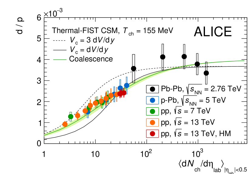
(a) (Anti)deuterons

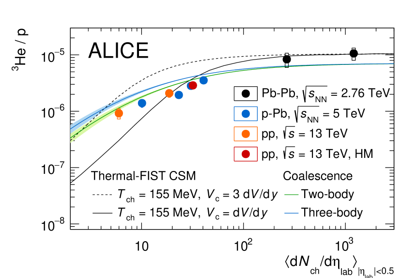
(b) (Anti)helions

Figure 6: Ratio between the $p_{\rm T}$-integrated yields of nuclei and protons as a function of multiplicity for (anti)deuterons (a) and (anti)helions (b). Measurements are performed in HM pp collisions at $\sqrt{s}~{}=~{}13$ TeV, in MB pp collisions at $\sqrt{s}~{}=~{}13$ TeV [17] and at $\sqrt{s}~{}=~{}7$ TeV [11], in p–Pb collisions at $\sqrt{s_{\mathrm{NN}}}~{}=~{}5.02$ TeV [15, 16], and in Pb–Pb collisions at $\sqrt{s_{\mathrm{NN}}}~{}=~{}2.76$ TeV [10]. Vertical bars and boxes represent statistical and systematic uncertainties, respectively. The two black lines are the theoretical predictions of the Thermal-FIST CSM [61] for two sizes of the correlation volume $V_{\mathrm{C}}$. For (anti)deuterons, the green line represents the expectation from a coalescence model [33]. For (anti)helion, the blue and green lines represent the expectations from a two-body and three-body coalescence model, respectively [33].

5 Summary

In this paper, the measurements of the production yields of (anti)nuclei in minimum bias and high-multiplicity pp collisions at $\sqrt{s}=$ 13 TeV are reported.

A significant increase of the coalescence parameter $B_{2}$ with increasing $p_{\rm T}/A$ is observed for the first time in pp collisions. Indeed, previous measurements in small collision systems were consistent with a flat trend within uncertainties. Given the very narrow multiplicity intervals used in the present measurement, this rising trend cannot be attributed to effects coming from a different hardening of the proton and deuteron spectra within the measured multiplicity intervals and thus points to some other physics effect. Moreover, the coalescence parameters are compared with theoretical calculations based on the coalescence approach using different internal wave functions of nuclei. This comparison was possible due to the availability of the measurement of the source radii in the same data sample. While the predictions for $B_{2}$ using a Gaussian approximation for the deuteron wave function are in very good agreement with the experimental results, for $B_{3}$ they overestimate the data by up to a factor of 2 at the lowest $p_{\rm T}$. Updated theoretical calculations including also more complex wave functions for ³He would help in providing a better description of this measurement.

The multiplicity evolution of the coalescence parameters for a fixed $p_{\rm T}/A$ and of the ratios of integrated yields d$/$p and ³He$/$p are consistent with the global trend from previous measurements. Moreover, the d$/$p ratio is consistent with predictions from the coalescence model, while significant deviations are observed between the ³He$/$p and coalescence expectations at intermediate multiplicities. The canonical statistical model predictions provide a qualitative description of the particle ratios presented in this paper at low and intermediate multiplicities covered by pp and p–Pb collisions and are consistent with the data only in the grand-canonical limit (multiplicities covered by Pb–Pb collisions).

Appendix A Theoretical prediction for the coalescence parameter $B_{A}$

In this appendix, the details about the theoretical prediction used for the coalescence parameter $B_{A}$ as a function of the source radius are reported. The general recipe is taken from Ref. [36]. $B_{2}$ is defined as

$$B_{2}(p)\approx\frac{3}{2m}\int\mathrm{d}^{3}q\,D(\vec{q})\,\mathcal{C}_{2}^{\mathrm{PRF}}\left(\vec{p},\vec{q}\right),$$ (3)

where $m$ is the proton mass, $p$ is the momentum of the nucleus, $q$ is the relative momentum of the nucleons, $D(\vec{q})$ is the deuteron Wigner density and $\mathcal{C}_{2}^{\mathrm{PRF}}\left(\vec{p},\vec{q}\right)$ is the correlation between two nucleons in the rest frame of the pair (PRF), assuming a Gaussian source model. For these calculations, we assume a homogeneous source, i.e. $R=R_{\parallel}=R_{\perp}$. Hence, the correlation function has the form

$$\mathcal{C}_{2}^{\mathrm{PRF}}\left(\vec{p},\vec{q}\right)=e^{-R^{2}q^{2}},$$ (4)

where $R$ is the source radius. Finally, the Wigner density is defined as

$$D(\vec{q})=\int\mathrm{d}^{3}r\,|\phi_{\mathrm{d}}(\vec{r})|^{2}e^{-i\vec{q}\times\vec{r}},$$ (5)

where $\phi_{\mathrm{d}}$ is the deuteron wave function. In the following, we will provide different predictions for $B_{2}$ as a function of the source radius $R$ starting from Eq. 3 and using different wave functions $\phi_{\mathrm{d}}$. The theoretical predictions for $B_{2}$ as a function of the source radius $R$ is shown in Fig. 7(a). At large values of the source radius they all show the same trend. On the contrary, for small values they differ, with a maximum spread of around a factor of 10. Eq. 3 has not an equivalent for $B_{3}$ and ab initio calculations are needed. For this reason, it is currently not possible to obtain $B_{3}$ predictions for different wave functions as easily as for $B_{2}$. However, it is possible to obtain a prediction for the case of a simple Gaussian wave function (see Eq. 9).

A.1 Gaussian wave function

The most simple assumption is a Gaussian wave function

$$\phi_{\mathrm{d}}(r)=\frac{e^{-\frac{r^{2}}{2d^{2}}}}{\left(\pi d^{2}\right)^{3/4}},$$ (6)

where $d$ is the nucleus radius. For this calculations, $d=3.2$ fm, as in Ref. [36]. The corresponding Wigner density is

$$D(\vec{q})=e^{-\frac{q^{2}d^{2}}{4}}.$$ (7)

This brings to the expression for $B_{2}$ as a function of the source radius $R$

$$B_{2}(R)=\frac{3\pi^{2}}{2m\left[R^{2}+\left(\frac{d}{2}\right)^{2}\right]^{\frac{3}{2}}}.$$ (8)

This function is shown in Fig. 7(a), together with the other predictions for $B_{2}$. As shown in Ref. [36], Eq. 8 can also be generalised for a nucleus with mass number $A$

$$B_{A}(R)=\frac{2J_{A}+1}{2^{A}\sqrt{A}}\frac{1}{m^{A-1}}\left[\frac{2\pi}{R^{2}+\left(r_{A}/2\right)^{2}}\right]^{\frac{3}{2}(A-1)},$$ (9)

where $J_{A}$ is the spin of the nucleus. Eq. 9 is used to calculate the theoretical prediction for $B_{3}$, shown in Fig. 7(b).

A.2 Hulthen wave function

The second hypothesis tested here is a Hulthen wave function

$$\phi_{\mathrm{d}}(r)=\sqrt{\frac{\alpha\beta(\alpha+\beta)}{2\pi(\alpha-\beta)^{2}}}\,\frac{e^{-\alpha r}-e^{-\beta r}}{r},$$ (10)

where $\alpha=0.2~{}\text{fm}^{-1}$ and $\beta=1.56~{}\text{fm}^{-1}$ are parameters taken from Ref. [32]. The corresponding expression for $B_{2}$ is

$$B_{2}(R)=\frac{3\pi^{2}}{R^{2}}\frac{\alpha\beta(\alpha+\beta)}{(\alpha-\beta)^{2}}\left[e^{4\alpha^{2}R^{2}}\text{erfc}(2\alpha R)-2e^{(\alpha+\beta)^{2}R^{2}}\text{erfc}((\alpha+\beta)R)+e^{4\beta^{2}R^{2}}\text{erfc}(2\beta R)\right].$$ (11)

This function is shown in Fig. 7(a), together with the other predictions for $B_{2}$.

A.3 Chiral Effective Field Theory wave function

The third hypothesis for deuteron wave function is obtained from Chiral Effective field theory ($\chi\text{EFT}$) calculations ($\text{N}^{4}\text{LO}$). It is based on Ref. [57] and the normalisation is based on Ref. [65]. A cutoff at $\Lambda_{c}=500$ MeV is used. The deuteron wave function is

$$\phi_{\mathrm{d}}(\vec{r})=\frac{1}{\sqrt{4\pi}\,r}\left[u(r)\,+\,\frac{1}{\sqrt{8}}\,w(r)\,S_{12}(\hat{r})\right]\,\chi_{1m}\,,$$ (12)

where $u(r)$ and $w(r)$ are radial wave functions, $S_{12}(\hat{r})$ is the spin tensor and $\chi_{1m}$ is a spinor. The spin-averaged density of the deuteron can be hence expressed as

$$\left|\phi_{\mathrm{d}}(r)\right|^{2}=\frac{1}{4\pi\,r^{2}}\left[u^{2}(r)\,+\,w^{2}(r)\right].$$ (13)

Using Eq. 3 and Eq. 5, one obtains

$$B_{2}(R)=\frac{6\pi}{m}\int_{0}^{\Lambda_{c}}\mathrm{d}q\int_{0}^{\infty}\mathrm{d}r\,q\,\left[u(r)^{2}\,+\,w(r)^{2}\right]\,\frac{\sin(qr)}{r}\,e^{-R^{2}q^{2}}.$$ (14)

Integrating Eq. 14 over $q$, one obtains

$$B_{2}(R)=\frac{3\pi}{mR^{2}}\int_{0}^{\infty}\,\frac{\mathrm{d}r}{r}\,\left[u^{2}(r)\,+\,w^{2}(r)\right]\,\left\{e^{-\Lambda_{c}^{2}R^{2}}\sin(\Lambda_{c}r)\,+\,\frac{\sqrt{\pi}r}{4R}\,e^{-\frac{r^{2}}{4R^{2}}}\,\left[\operatorname{erf}\left(\frac{ir+2R^{2}\Lambda_{c}}{2R}\right)\,-\,\operatorname{erf}\left(\frac{ir-2R^{2}\Lambda_{c}}{2R}\right)\right]\right\}\,.$$ (15)

This function is shown in Fig. 7(a), together with the other predictions for $B_{2}$.

A.4 Combination of two Gaussians

The last considered wave function is a combination of two Gaussians, fitted to the Hulthen wave function [34]:

$$\phi_{\mathrm{d}}(r)=\pi^{-3/4}\left[\frac{\Delta^{1/2}}{d_{1}^{3/2}}e^{-r^{2}/(2d_{1}^{2})}\;+\;e^{i\alpha}\frac{(1-\Delta)^{1/2}}{d_{2}^{3/2}}e^{-r^{2}/(2d_{2}^{2})}\right]$$ (16)

, where $\Delta=0.581$, $d_{1}=3.979$ fm and $d_{1}=0.890$ fm. The corresponding density is

$$|\phi_{\mathrm{d}}(r)|^{2}={\pi^{-3/2}}\left[\frac{\Delta}{d_{1}^{3}}e^{-r^{2}/d_{1}^{2}}+\frac{1-\Delta}{d_{2}^{3}}e^{-r^{2}/d_{2}^{2}}\right]\,.$$ (17)

$B_{2}$ can be hence written as

$$B_{2}(R)=\frac{24\pi^{5/2}}{m}\int_{0}^{\infty}\,\mathrm{d}q\int_{0}^{\infty}\,\mathrm{d}r\,|\phi_{d}(r)|^{2}\,\sin(qr)\,r\,q\,e^{-R^{2}q^{2}}\,,$$ (18)

and after integrating over $q$ and $r$, one obtains:

$$B_{2}(R)=\frac{3\pi^{3/2}}{2mR^{3}}\left[\Delta\,\left(1\,+\,\frac{d_{1}^{2}}{4R^{2}}\right)^{-3/2}\,+\,(1\,-\,\Delta)\,\left(1\,+\,\frac{d_{2}^{2}}{4R^{2}}\right)^{-3/2}\,\right]\,.$$ (19)

This function is shown in Fig. 7(a), together with the other predictions for $B_{2}$.

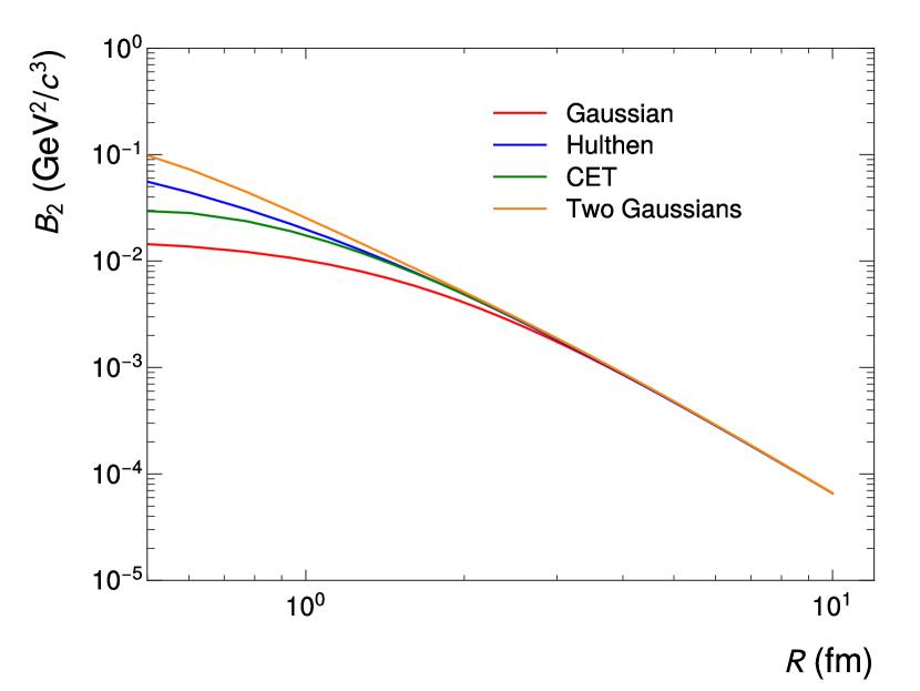
(a)

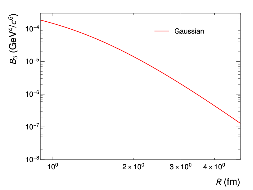
(b)

Figure 7: Coalescence parameters $B_{2}$ (a) and $B_{3}$ (b) as a function of the source radius $R$ for different wave functions (see the text for more details).

Appendix B The ALICE Collaboration

S. Acharya¹⁴⁴, D. Adamová⁹⁸, A. Adler⁷⁶, J. Adolfsson⁸³, G. Aglieri Rinella³⁵, M. Agnello³¹, N. Agrawal⁵⁵, Z. Ahammed¹⁴⁴, S. Ahmad¹⁶, S.U. Ahn⁷⁸, I. Ahuja³⁹, Z. Akbar⁵², A. Akindinov⁹⁵, M. Al-Turany¹¹¹, S.N. Alam^16,41, D. Aleksandrov⁹¹, B. Alessandro⁶¹, H.M. Alfanda⁷, R. Alfaro Molina⁷³, B. Ali¹⁶, Y. Ali¹⁴, A. Alici²⁶, N. Alizadehvandchali¹²⁸, A. Alkin³⁵, J. Alme²¹, T. Alt⁷⁰, L. Altenkamper²¹, I. Altsybeev¹¹⁶, M.N. Anaam⁷, C. Andrei⁴⁹, D. Andreou⁹³, A. Andronic¹⁴⁷, M. Angeletti³⁵, V. Anguelov¹⁰⁷, F. Antinori⁵⁸, P. Antonioli⁵⁵, C. Anuj¹⁶, N. Apadula⁸², L. Aphecetche¹¹⁸, H. Appelshäuser⁷⁰, S. Arcelli²⁶, R. Arnaldi⁶¹, I.C. Arsene²⁰, M. Arslandok^149,107, A. Augustinus³⁵, R. Averbeck¹¹¹, S. Aziz⁸⁰, M.D. Azmi¹⁶, A. Badalà⁵⁷, Y.W. Baek⁴², X. Bai^132,111, R. Bailhache⁷⁰, Y. Bailung⁵¹, R. Bala¹⁰⁴, A. Balbino³¹, A. Baldisseri¹⁴¹, B. Balis², D. Banerjee⁴, R. Barbera²⁷, L. Barioglio¹⁰⁸, M. Barlou⁸⁷, G.G. Barnaföldi¹⁴⁸, L.S. Barnby⁹⁷, V. Barret¹³⁸, C. Bartels¹³¹, K. Barth³⁵, E. Bartsch⁷⁰, F. Baruffaldi²⁸, N. Bastid¹³⁸, S. Basu⁸³, G. Batigne¹¹⁸, B. Batyunya⁷⁷, D. Bauri⁵⁰, J.L. Bazo Alba¹¹⁵, I.G. Bearden⁹², C. Beattie¹⁴⁹, I. Belikov¹⁴⁰, A.D.C. Bell Hechavarria¹⁴⁷, F. Bellini²⁶, R. Bellwied¹²⁸, S. Belokurova¹¹⁶, V. Belyaev⁹⁶, G. Bencedi^148,71, S. Beole²⁵, A. Bercuci⁴⁹, Y. Berdnikov¹⁰¹, A. Berdnikova¹⁰⁷, L. Bergmann¹⁰⁷, M.G. Besoiu⁶⁹, L. Betev³⁵, P.P. Bhaduri¹⁴⁴, A. Bhasin¹⁰⁴, I.R. Bhat¹⁰⁴, M.A. Bhat⁴, B. Bhattacharjee⁴³, P. Bhattacharya²³, L. Bianchi²⁵, N. Bianchi⁵³, J. Bielčík³⁸, J. Bielčíková⁹⁸, J. Biernat¹²¹, A. Bilandzic¹⁰⁸, G. Biro¹⁴⁸, S. Biswas⁴, J.T. Blair¹²², D. Blau^91,84, M.B. Blidaru¹¹¹, C. Blume⁷⁰, G. Boca^29,59, F. Bock⁹⁹, A. Bogdanov⁹⁶, S. Boi²³, J. Bok⁶³, L. Boldizsár¹⁴⁸, A. Bolozdynya⁹⁶, M. Bombara³⁹, P.M. Bond³⁵, G. Bonomi^143,59, H. Borel¹⁴¹, A. Borissov⁸⁴, H. Bossi¹⁴⁹, E. Botta²⁵, L. Bratrud⁷⁰, P. Braun-Munzinger¹¹¹, M. Bregant¹²⁴, M. Broz³⁸, G.E. Bruno^110,34, M.D. Buckland¹³¹, D. Budnikov¹¹², H. Buesching⁷⁰, S. Bufalino³¹, O. Bugnon¹¹⁸, P. Buhler¹¹⁷, Z. Buthelezi^74,135, J.B. Butt¹⁴, A. Bylinkin¹³⁰, S.A. Bysiak¹²¹, M. Cai^28,7, H. Caines¹⁴⁹, A. Caliva¹¹¹, E. Calvo Villar¹¹⁵, J.M.M. Camacho¹²³, R.S. Camacho⁴⁶, P. Camerini²⁴, F.D.M. Canedo¹²⁴, F. Carnesecchi^35,26, R. Caron¹⁴¹, J. Castillo Castellanos¹⁴¹, E.A.R. Casula²³, F. Catalano³¹, C. Ceballos Sanchez⁷⁷, P. Chakraborty⁵⁰, S. Chandra¹⁴⁴, S. Chapeland³⁵, M. Chartier¹³¹, S. Chattopadhyay¹⁴⁴, S. Chattopadhyay¹¹³, A. Chauvin²³, T.G. Chavez⁴⁶, T. Cheng⁷, C. Cheshkov¹³⁹, B. Cheynis¹³⁹, V. Chibante Barroso³⁵, D.D. Chinellato¹²⁵, S. Cho⁶³, P. Chochula³⁵, P. Christakoglou⁹³, C.H. Christensen⁹², P. Christiansen⁸³, T. Chujo¹³⁷, C. Cicalo⁵⁶, L. Cifarelli²⁶, F. Cindolo⁵⁵, M.R. Ciupek¹¹¹, G. Clai^II,55, J. Cleymans^I,127, F. Colamaria⁵⁴, J.S. Colburn¹¹⁴, D. Colella^{110,54,34,148}, A. Collu⁸², M. Colocci³⁵, M. Concas^III,61, G. Conesa Balbastre⁸¹, Z. Conesa del Valle⁸⁰, G. Contin²⁴, J.G. Contreras³⁸, M.L. Coquet¹⁴¹, T.M. Cormier⁹⁹, P. Cortese³², M.R. Cosentino¹²⁶, F. Costa³⁵, S. Costanza^29,59, P. Crochet¹³⁸, R. Cruz-Torres⁸², E. Cuautle⁷¹, P. Cui⁷, L. Cunqueiro⁹⁹, A. Dainese⁵⁸, M.C. Danisch¹⁰⁷, A. Danu⁶⁹, I. Das¹¹³, P. Das⁸⁹, P. Das⁴, S. Das⁴, S. Dash⁵⁰, S. De⁸⁹, A. De Caro³⁰, G. de Cataldo⁵⁴, L. De Cilladi²⁵, J. de Cuveland⁴⁰, A. De Falco²³, D. De Gruttola³⁰, N. De Marco⁶¹, C. De Martin²⁴, S. De Pasquale³⁰, S. Deb⁵¹, H.F. Degenhardt¹²⁴, K.R. Deja¹⁴⁵, L. Dello Stritto³⁰, W. Deng⁷, P. Dhankher¹⁹, D. Di Bari³⁴, A. Di Mauro³⁵, R.A. Diaz⁸, T. Dietel¹²⁷, Y. Ding^139,7, R. Divià³⁵, D.U. Dixit¹⁹, Ø. Djuvsland²¹, U. Dmitrieva⁶⁵, J. Do⁶³, A. Dobrin⁶⁹, B. Dönigus⁷⁰, O. Dordic²⁰, A.K. Dubey¹⁴⁴, A. Dubla^111,93, S. Dudi¹⁰³, M. Dukhishyam⁸⁹, P. Dupieux¹³⁸, N. Dzalaiova¹³, T.M. Eder¹⁴⁷, R.J. Ehlers⁹⁹, V.N. Eikeland²¹, F. Eisenhut⁷⁰, D. Elia⁵⁴, B. Erazmus¹¹⁸, F. Ercolessi²⁶, F. Erhardt¹⁰², A. Erokhin¹¹⁶, M.R. Ersdal²¹, B. Espagnon⁸⁰, G. Eulisse³⁵, D. Evans¹¹⁴, S. Evdokimov⁹⁴, L. Fabbietti¹⁰⁸, M. Faggin²⁸, J. Faivre⁸¹, F. Fan⁷, A. Fantoni⁵³, M. Fasel⁹⁹, P. Fecchio³¹, A. Feliciello⁶¹, G. Feofilov¹¹⁶, A. Fernández Téllez⁴⁶, A. Ferrero¹⁴¹, A. Ferretti²⁵, V.J.G. Feuillard¹⁰⁷, J. Figiel¹²¹, S. Filchagin¹¹², D. Finogeev⁶⁵, F.M. Fionda^56,21, G. Fiorenza^35,110, F. Flor¹²⁸, A.N. Flores¹²², S. Foertsch⁷⁴, P. Foka¹¹¹, S. Fokin⁹¹, E. Fragiacomo⁶², E. Frajna¹⁴⁸, U. Fuchs³⁵, N. Funicello³⁰, C. Furget⁸¹, A. Furs⁶⁵, J.J. Gaardhøje⁹², M. Gagliardi²⁵, A.M. Gago¹¹⁵, A. Gal¹⁴⁰, C.D. Galvan¹²³, P. Ganoti⁸⁷, C. Garabatos¹¹¹, J.R.A. Garcia⁴⁶, E. Garcia-Solis¹⁰, K. Garg¹¹⁸, C. Gargiulo³⁵, A. Garibli⁹⁰, K. Garner¹⁴⁷, P. Gasik¹¹¹, E.F. Gauger¹²², A. Gautam¹³⁰, M.B. Gay Ducati⁷², M. Germain¹¹⁸, P. Ghosh¹⁴⁴, S.K. Ghosh⁴, M. Giacalone²⁶, P. Gianotti⁵³, P. Giubellino^111,61, P. Giubilato²⁸, A.M.C. Glaenzer¹⁴¹, P. Glässel¹⁰⁷, D.J.Q. Goh⁸⁵, V. Gonzalez¹⁴⁶, L.H. González-Trueba⁷³, S. Gorbunov⁴⁰, M. Gorgon², L. Görlich¹²¹, S. Gotovac³⁶, V. Grabski⁷³, L.K. Graczykowski¹⁴⁵, L. Greiner⁸², A. Grelli⁶⁴, C. Grigoras³⁵, V. Grigoriev⁹⁶, S. Grigoryan^77,1, F. Grosa^35,61, J.F. Grosse-Oetringhaus³⁵, R. Grosso¹¹¹, G.G. Guardiano¹²⁵, R. Guernane⁸¹, M. Guilbaud¹¹⁸, K. Gulbrandsen⁹², T. Gunji¹³⁶, W. Guo⁷, A. Gupta¹⁰⁴, R. Gupta¹⁰⁴, S.P. Guzman⁴⁶, L. Gyulai¹⁴⁸, M.K. Habib¹¹¹, C. Hadjidakis⁸⁰, G. Halimoglu⁷⁰, H. Hamagaki⁸⁵, M. Hamid⁷, R. Hannigan¹²², M.R. Haque^145,89, A. Harlenderova¹¹¹, J.W. Harris¹⁴⁹, A. Harton¹⁰, J.A. Hasenbichler³⁵, H. Hassan⁹⁹, D. Hatzifotiadou⁵⁵, P. Hauer⁴⁴, L.B. Havener¹⁴⁹, S.T. Heckel¹⁰⁸, E. Hellbär¹¹¹, H. Helstrup³⁷, T. Herman³⁸, E.G. Hernandez⁴⁶, G. Herrera Corral⁹, F. Herrmann¹⁴⁷, K.F. Hetland³⁷, H. Hillemanns³⁵, C. Hills¹³¹, B. Hippolyte¹⁴⁰, B. Hofman⁶⁴, B. Hohlweger⁹³, J. Honermann¹⁴⁷, G.H. Hong¹⁵⁰, D. Horak³⁸, S. Hornung¹¹¹, A. Horzyk², R. Hosokawa¹⁵, Y. Hou⁷, P. Hristov³⁵, C. Hughes¹³⁴, P. Huhn⁷⁰, L.M. Huhta¹²⁹, T.J. Humanic¹⁰⁰, H. Hushnud¹¹³, L.A. Husova¹⁴⁷, A. Hutson¹²⁸, D. Hutter⁴⁰, J.P. Iddon^35,131, R. Ilkaev¹¹², H. Ilyas¹⁴, M. Inaba¹³⁷, G.M. Innocenti³⁵, M. Ippolitov⁹¹, A. Isakov^38,98, M.S. Islam¹¹³, M. Ivanov¹¹¹, V. Ivanov¹⁰¹, V. Izucheev⁹⁴, M. Jablonski², B. Jacak⁸², N. Jacazio³⁵, P.M. Jacobs⁸², S. Jadlovska¹²⁰, J. Jadlovsky¹²⁰, S. Jaelani⁶⁴, C. Jahnke^125,124, M.J. Jakubowska¹⁴⁵, A. Jalotra¹⁰⁴, M.A. Janik¹⁴⁵, T. Janson⁷⁶, M. Jercic¹⁰², O. Jevons¹¹⁴, A.A.P. Jimenez⁷¹, F. Jonas^99,147, P.G. Jones¹¹⁴, J.M. Jowett ^35,111, J. Jung⁷⁰, M. Jung⁷⁰, A. Junique³⁵, A. Jusko¹¹⁴, J. Kaewjai¹¹⁹, P. Kalinak⁶⁶, A.S. Kalteyer¹¹¹, A. Kalweit³⁵, V. Kaplin⁹⁶, A. Karasu Uysal⁷⁹, D. Karatovic¹⁰², O. Karavichev⁶⁵, T. Karavicheva⁶⁵, P. Karczmarczyk¹⁴⁵, E. Karpechev⁶⁵, A. Kazantsev⁹¹, U. Kebschull⁷⁶, R. Keidel⁴⁸, D.L.D. Keijdener⁶⁴, M. Keil³⁵, B. Ketzer⁴⁴, Z. Khabanova⁹³, A.M. Khan⁷, S. Khan¹⁶, A. Khanzadeev¹⁰¹, Y. Kharlov^94,84, A. Khatun¹⁶, A. Khuntia¹²¹, B. Kileng³⁷, B. Kim^17,63, C. Kim¹⁷, D.J. Kim¹²⁹, E.J. Kim⁷⁵, J. Kim¹⁵⁰, J.S. Kim⁴², J. Kim¹⁰⁷, J. Kim¹⁵⁰, J. Kim⁷⁵, M. Kim¹⁰⁷, S. Kim¹⁸, T. Kim¹⁵⁰, S. Kirsch⁷⁰, I. Kisel⁴⁰, S. Kiselev⁹⁵, A. Kisiel¹⁴⁵, J.P. Kitowski², J.L. Klay⁶, J. Klein³⁵, S. Klein⁸², C. Klein-Bösing¹⁴⁷, M. Kleiner⁷⁰, T. Klemenz¹⁰⁸, A. Kluge³⁵, A.G. Knospe¹²⁸, C. Kobdaj¹¹⁹, M.K. Köhler¹⁰⁷, T. Kollegger¹¹¹, A. Kondratyev⁷⁷, N. Kondratyeva⁹⁶, E. Kondratyuk⁹⁴, J. Konig⁷⁰, S.A. Konigstorfer¹⁰⁸, P.J. Konopka³⁵, G. Kornakov¹⁴⁵, S.D. Koryciak², A. Kotliarov⁹⁸, O. Kovalenko⁸⁸, V. Kovalenko¹¹⁶, M. Kowalski¹²¹, I. Králik⁶⁶, A. Kravčáková³⁹, L. Kreis¹¹¹, M. Krivda^114,66, F. Krizek⁹⁸, K. Krizkova Gajdosova³⁸, M. Kroesen¹⁰⁷, M. Krüger⁷⁰, E. Kryshen¹⁰¹, M. Krzewicki⁴⁰, V. Kučera³⁵, C. Kuhn¹⁴⁰, P.G. Kuijer⁹³, T. Kumaoka¹³⁷, D. Kumar¹⁴⁴, L. Kumar¹⁰³, N. Kumar¹⁰³, S. Kundu³⁵, P. Kurashvili⁸⁸, A. Kurepin⁶⁵, A.B. Kurepin⁶⁵, A. Kuryakin¹¹², S. Kushpil⁹⁸, J. Kvapil¹¹⁴, M.J. Kweon⁶³, J.Y. Kwon⁶³, Y. Kwon¹⁵⁰, S.L. La Pointe⁴⁰, P. La Rocca²⁷, Y.S. Lai⁸², A. Lakrathok¹¹⁹, M. Lamanna³⁵, R. Langoy¹³³, K. Lapidus³⁵, P. Larionov^35,53, E. Laudi³⁵, L. Lautner^35,108, R. Lavicka^117,38, T. Lazareva¹¹⁶, R. Lea^143,24,59, J. Lehrbach⁴⁰, R.C. Lemmon⁹⁷, I. León Monzón¹²³, E.D. Lesser¹⁹, M. Lettrich^35,108, P. Lévai¹⁴⁸, X. Li¹¹, X.L. Li⁷, J. Lien¹³³, R. Lietava¹¹⁴, B. Lim¹⁷, S.H. Lim¹⁷, V. Lindenstruth⁴⁰, A. Lindner⁴⁹, C. Lippmann¹¹¹, A. Liu¹⁹, D.H. Liu⁷, J. Liu¹³¹, I.M. Lofnes²¹, V. Loginov⁹⁶, C. Loizides⁹⁹, P. Loncar³⁶, J.A. Lopez¹⁰⁷, X. Lopez¹³⁸, E. López Torres⁸, J.R. Luhder¹⁴⁷, M. Lunardon²⁸, G. Luparello⁶², Y.G. Ma⁴¹, A. Maevskaya⁶⁵, M. Mager³⁵, T. Mahmoud⁴⁴, A. Maire¹⁴⁰, M. Malaev¹⁰¹, N.M. Malik¹⁰⁴, Q.W. Malik²⁰, S.K. Malik¹⁰⁴, L. Malinina^IV,77, D. Mal’Kevich⁹⁵, N. Mallick⁵¹, P. Malzacher¹¹¹, G. Mandaglio^33,57, V. Manko⁹¹, F. Manso¹³⁸, V. Manzari⁵⁴, Y. Mao⁷, J. Mareš⁶⁸, G.V. Margagliotti²⁴, A. Margotti⁵⁵, A. Marín¹¹¹, C. Markert¹²², M. Marquard⁷⁰, N.A. Martin¹⁰⁷, P. Martinengo³⁵, J.L. Martinez¹²⁸, M.I. Martínez⁴⁶, G. Martínez García¹¹⁸, S. Masciocchi¹¹¹, M. Masera²⁵, A. Masoni⁵⁶, L. Massacrier⁸⁰, A. Mastroserio^142,54, A.M. Mathis¹⁰⁸, O. Matonoha⁸³, P.F.T. Matuoka¹²⁴, A. Matyja¹²¹, C. Mayer¹²¹, A.L. Mazuecos³⁵, F. Mazzaschi²⁵, M. Mazzilli³⁵, M.A. Mazzoni^I,60, J.E. Mdhluli¹³⁵, A.F. Mechler⁷⁰, F. Meddi²², Y. Melikyan⁶⁵, A. Menchaca-Rocha⁷³, E. Meninno^117,30, A.S. Menon¹²⁸, M. Meres¹³, S. Mhlanga^127,74, Y. Miake¹³⁷, L. Micheletti⁶¹, L.C. Migliorin¹³⁹, D.L. Mihaylov¹⁰⁸, K. Mikhaylov^77,95, A.N. Mishra¹⁴⁸, D. Miśkowiec¹¹¹, A. Modak⁴, A.P. Mohanty⁶⁴, B. Mohanty⁸⁹, M. Mohisin Khan^V,16, M.A. Molander⁴⁵, Z. Moravcova⁹², C. Mordasini¹⁰⁸, D.A. Moreira De Godoy¹⁴⁷, I. Morozov⁶⁵, A. Morsch³⁵, T. Mrnjavac³⁵, V. Muccifora⁵³, E. Mudnic³⁶, B.J. Mughal¹⁰⁹, D. Mühlheim¹⁴⁷, S. Muhuri¹⁴⁴, J.D. Mulligan⁸², A. Mulliri²³, M.G. Munhoz¹²⁴, R.H. Munzer⁷⁰, H. Murakami¹³⁶, S. Murray¹²⁷, L. Musa³⁵, J. Musinsky⁶⁶, J.W. Myrcha¹⁴⁵, B. Naik^135,50, R. Nair⁸⁸, B.K. Nandi⁵⁰, R. Nania⁵⁵, E. Nappi⁵⁴, A.F. Nassirpour⁸³, A. Nath¹⁰⁷, C. Nattrass¹³⁴, A. Neagu²⁰, L. Nellen⁷¹, S.V. Nesbo³⁷, G. Neskovic⁴⁰, D. Nesterov¹¹⁶, B.S. Nielsen⁹², S. Nikolaev⁹¹, S. Nikulin⁹¹, V. Nikulin¹⁰¹, F. Noferini⁵⁵, S. Noh¹², P. Nomokonov⁷⁷, J. Norman¹³¹, N. Novitzky¹³⁷, P. Nowakowski¹⁴⁵, A. Nyanin⁹¹, J. Nystrand²¹, M. Ogino⁸⁵, A. Ohlson⁸³, V.A. Okorokov⁹⁶, J. Oleniacz¹⁴⁵, A.C. Oliveira Da Silva¹³⁴, M.H. Oliver¹⁴⁹, A. Onnerstad¹²⁹, C. Oppedisano⁶¹, A. Ortiz Velasquez⁷¹, T. Osako⁴⁷, A. Oskarsson⁸³, J. Otwinowski¹²¹, M. Oya⁴⁷, K. Oyama⁸⁵, Y. Pachmayer¹⁰⁷, S. Padhan⁵⁰, D. Pagano^143,59, G. Paić⁷¹, A. Palasciano⁵⁴, J. Pan¹⁴⁶, S. Panebianco¹⁴¹, P. Pareek¹⁴⁴, J. Park⁶³, J.E. Parkkila¹²⁹, S.P. Pathak¹²⁸, R.N. Patra^104,35, B. Paul²³, H. Pei⁷, T. Peitzmann⁶⁴, X. Peng⁷, L.G. Pereira⁷², H. Pereira Da Costa¹⁴¹, D. Peresunko^91,84, G.M. Perez⁸, S. Perrin¹⁴¹, Y. Pestov⁵, V. Petráček³⁸, M. Petrovici⁴⁹, R.P. Pezzi^118,72, S. Piano⁶², M. Pikna¹³, P. Pillot¹¹⁸, O. Pinazza^55,35, L. Pinsky¹²⁸, C. Pinto²⁷, S. Pisano⁵³, M. Płoskoń⁸², M. Planinic¹⁰², F. Pliquett⁷⁰, M.G. Poghosyan⁹⁹, B. Polichtchouk⁹⁴, S. Politano³¹, N. Poljak¹⁰², A. Pop⁴⁹, S. Porteboeuf-Houssais¹³⁸, J. Porter⁸², V. Pozdniakov⁷⁷, S.K. Prasad⁴, R. Preghenella⁵⁵, F. Prino⁶¹, C.A. Pruneau¹⁴⁶, I. Pshenichnov⁶⁵, M. Puccio³⁵, S. Qiu⁹³, L. Quaglia²⁵, R.E. Quishpe¹²⁸, S. Ragoni¹¹⁴, A. Rakotozafindrabe¹⁴¹, L. Ramello³², F. Rami¹⁴⁰, S.A.R. Ramirez⁴⁶, A.G.T. Ramos³⁴, T.A. Rancien⁸¹, R. Raniwala¹⁰⁵, S. Raniwala¹⁰⁵, S.S. Räsänen⁴⁵, R. Rath⁵¹, I. Ravasenga⁹³, K.F. Read^99,134, A.R. Redelbach⁴⁰, K. Redlich^VI,88, A. Rehman²¹, P. Reichelt⁷⁰, F. Reidt³⁵, H.A. Reme-ness³⁷, R. Renfordt⁷⁰, Z. Rescakova³⁹, K. Reygers¹⁰⁷, A. Riabov¹⁰¹, V. Riabov¹⁰¹, T. Richert⁸³, M. Richter²⁰, W. Riegler³⁵, F. Riggi²⁷, C. Ristea⁶⁹, M. Rodríguez Cahuantzi⁴⁶, K. Røed²⁰, R. Rogalev⁹⁴, E. Rogochaya⁷⁷, T.S. Rogoschinski⁷⁰, D. Rohr³⁵, D. Röhrich²¹, P.F. Rojas⁴⁶, P.S. Rokita¹⁴⁵, F. Ronchetti⁵³, A. Rosano^33,57, E.D. Rosas⁷¹, A. Rossi⁵⁸, A. Rotondi^29,59, A. Roy⁵¹, P. Roy¹¹³, S. Roy⁵⁰, N. Rubini²⁶, O.V. Rueda⁸³, D. Ruggiano¹⁴⁵, R. Rui²⁴, B. Rumyantsev⁷⁷, P.G. Russek², R. Russo⁹³, A. Rustamov⁹⁰, E. Ryabinkin⁹¹, Y. Ryabov¹⁰¹, A. Rybicki¹²¹, H. Rytkonen¹²⁹, W. Rzesa¹⁴⁵, O.A.M. Saarimaki⁴⁵, R. Sadek¹¹⁸, S. Sadovsky⁹⁴, J. Saetre²¹, K. Šafařík³⁸, S.K. Saha¹⁴⁴, S. Saha⁸⁹, B. Sahoo⁵⁰, P. Sahoo⁵⁰, R. Sahoo⁵¹, S. Sahoo⁶⁷, D. Sahu⁵¹, P.K. Sahu⁶⁷, J. Saini¹⁴⁴, S. Sakai¹³⁷, M.P. Salvan¹¹¹, S. Sambyal¹⁰⁴, V. Samsonov^I,101,96, D. Sarkar¹⁴⁶, N. Sarkar¹⁴⁴, P. Sarma⁴³, V.M. Sarti¹⁰⁸, M.H.P. Sas¹⁴⁹, J. Schambach⁹⁹, H.S. Scheid⁷⁰, C. Schiaua⁴⁹, R. Schicker¹⁰⁷, A. Schmah¹⁰⁷, C. Schmidt¹¹¹, H.R. Schmidt¹⁰⁶, M.O. Schmidt^35,107, M. Schmidt¹⁰⁶, N.V. Schmidt^99,70, A.R. Schmier¹³⁴, R. Schotter¹⁴⁰, J. Schukraft³⁵, K. Schwarz¹¹¹, K. Schweda¹¹¹, G. Scioli²⁶, E. Scomparin⁶¹, J.E. Seger¹⁵, Y. Sekiguchi¹³⁶, D. Sekihata¹³⁶, I. Selyuzhenkov^111,96, S. Senyukov¹⁴⁰, J.J. Seo⁶³, D. Serebryakov⁶⁵, L. Šerkšnytė¹⁰⁸, A. Sevcenco⁶⁹, T.J. Shaba⁷⁴, A. Shabanov⁶⁵, A. Shabetai¹¹⁸, R. Shahoyan³⁵, W. Shaikh¹¹³, A. Shangaraev⁹⁴, A. Sharma¹⁰³, H. Sharma¹²¹, M. Sharma¹⁰⁴, N. Sharma¹⁰³, S. Sharma¹⁰⁴, U. Sharma¹⁰⁴, O. Sheibani¹²⁸, K. Shigaki⁴⁷, M. Shimomura⁸⁶, S. Shirinkin⁹⁵, Q. Shou⁴¹, Y. Sibiriak⁹¹, S. Siddhanta⁵⁶, T. Siemiarczuk⁸⁸, T.F. Silva¹²⁴, D. Silvermyr⁸³, T. Simantathammakul¹¹⁹, G. Simonetti³⁵, B. Singh¹⁰⁸, R. Singh⁸⁹, R. Singh¹⁰⁴, R. Singh⁵¹, V.K. Singh¹⁴⁴, V. Singhal¹⁴⁴, T. Sinha¹¹³, B. Sitar¹³, M. Sitta³², T.B. Skaali²⁰, G. Skorodumovs¹⁰⁷, M. Slupecki⁴⁵, N. Smirnov¹⁴⁹, R.J.M. Snellings⁶⁴, C. Soncco¹¹⁵, J. Song¹²⁸, A. Songmoolnak¹¹⁹, F. Soramel²⁸, S. Sorensen¹³⁴, I. Sputowska¹²¹, J. Stachel¹⁰⁷, I. Stan⁶⁹, P.J. Steffanic¹³⁴, S.F. Stiefelmaier¹⁰⁷, D. Stocco¹¹⁸, I. Storehaug²⁰, M.M. Storetvedt³⁷, P. Stratmann¹⁴⁷, C.P. Stylianidis⁹³, A.A.P. Suaide¹²⁴, T. Sugitate⁴⁷, C. Suire⁸⁰, M. Sukhanov⁶⁵, M. Suljic³⁵, R. Sultanov⁹⁵, V. Sumberia¹⁰⁴, S. Sumowidagdo⁵², S. Swain⁶⁷, A. Szabo¹³, I. Szarka¹³, U. Tabassam¹⁴, S.F. Taghavi¹⁰⁸, G. Taillepied¹³⁸, J. Takahashi¹²⁵, G.J. Tambave²¹, S. Tang^138,7, Z. Tang¹³², J.D. Tapia Takaki^VII,130, M. Tarhini¹¹⁸, M.G. Tarzila⁴⁹, A. Tauro³⁵, G. Tejeda Muñoz⁴⁶, A. Telesca³⁵, L. Terlizzi²⁵, C. Terrevoli¹²⁸, G. Tersimonov³, S. Thakur¹⁴⁴, D. Thomas¹²², R. Tieulent¹³⁹, A. Tikhonov⁶⁵, A.R. Timmins¹²⁸, M. Tkacik¹²⁰, A. Toia⁷⁰, N. Topilskaya⁶⁵, M. Toppi⁵³, F. Torales-Acosta¹⁹, T. Tork⁸⁰, S.R. Torres³⁸, A. Trifiró^33,57, S. Tripathy^55,71, T. Tripathy⁵⁰, S. Trogolo^35,28, V. Trubnikov³, W.H. Trzaska¹²⁹, T.P. Trzcinski¹⁴⁵, B.A. Trzeciak³⁸, A. Tumkin¹¹², R. Turrisi⁵⁸, T.S. Tveter²⁰, K. Ullaland²¹, A. Uras¹³⁹, M. Urioni^59,143, G.L. Usai²³, M. Vala³⁹, N. Valle^29,59, S. Vallero⁶¹, N. van der Kolk⁶⁴, L.V.R. van Doremalen⁶⁴, M. van Leeuwen⁹³, P. Vande Vyvre³⁵, D. Varga¹⁴⁸, Z. Varga¹⁴⁸, M. Varga-Kofarago¹⁴⁸, M. Vasileiou⁸⁷, A. Vasiliev⁹¹, O. Vázquez Doce^53,108, V. Vechernin¹¹⁶, E. Vercellin²⁵, S. Vergara Limón⁴⁶, L. Vermunt⁶⁴, R. Vértesi¹⁴⁸, M. Verweij⁶⁴, L. Vickovic³⁶, Z. Vilakazi¹³⁵, O. Villalobos Baillie¹¹⁴, G. Vino⁵⁴, A. Vinogradov⁹¹, T. Virgili³⁰, V. Vislavicius⁹², A. Vodopyanov⁷⁷, B. Volkel^35,107, M.A. Völkl¹⁰⁷, K. Voloshin⁹⁵, S.A. Voloshin¹⁴⁶, G. Volpe³⁴, B. von Haller³⁵, I. Vorobyev¹⁰⁸, D. Voscek¹²⁰, N. Vozniuk⁶⁵, J. Vrláková³⁹, B. Wagner²¹, C. Wang⁴¹, D. Wang⁴¹, M. Weber¹¹⁷, R.J.G.V. Weelden⁹³, A. Wegrzynek³⁵, S.C. Wenzel³⁵, J.P. Wessels¹⁴⁷, J. Wiechula⁷⁰, J. Wikne²⁰, G. Wilk⁸⁸, J. Wilkinson¹¹¹, G.A. Willems¹⁴⁷, B. Windelband¹⁰⁷, M. Winn¹⁴¹, W.E. Witt¹³⁴, J.R. Wright¹²², W. Wu⁴¹, Y. Wu¹³², R. Xu⁷, A.K. Yadav¹⁴⁴, S. Yalcin⁷⁹, Y. Yamaguchi⁴⁷, K. Yamakawa⁴⁷, S. Yang²¹, S. Yano⁴⁷, Z. Yasin¹⁰⁹, Z. Yin⁷, H. Yokoyama⁶⁴, I.-K. Yoo¹⁷, J.H. Yoon⁶³, S. Yuan²¹, A. Yuncu¹⁰⁷, V. Zaccolo²⁴, C. Zampolli³⁵, H.J.C. Zanoli⁶⁴, N. Zardoshti³⁵, A. Zarochentsev¹¹⁶, P. Závada⁶⁸, N. Zaviyalov¹¹², M. Zhalov¹⁰¹, B. Zhang⁷, S. Zhang⁴¹, X. Zhang⁷, Y. Zhang¹³², V. Zherebchevskii¹¹⁶, Y. Zhi¹¹, N. Zhigareva⁹⁵, D. Zhou⁷, Y. Zhou⁹², J. Zhu^7,111, Y. Zhu⁷, A. Zichichi²⁶, G. Zinovjev³, N. Zurlo^143,59

Affiliation Notes

^I Deceased
^II Also at: Italian National Agency for New Technologies, Energy and Sustainable Economic Development (ENEA), Bologna, Italy
^III Also at: Dipartimento DET del Politecnico di Torino, Turin, Italy
^IV Also at: M.V. Lomonosov Moscow State University, D.V. Skobeltsyn Institute of Nuclear, Physics, Moscow, Russia
^V Also at: Department of Applied Physics, Aligarh Muslim University, Aligarh, India
^VI Also at: Institute of Theoretical Physics, University of Wroclaw, Poland
^VII Also at: University of Kansas, Lawrence, Kansas, United States

Collaboration Institutes

¹ A.I. Alikhanyan National Science Laboratory (Yerevan Physics Institute) Foundation, Yerevan, Armenia
² AGH University of Science and Technology, Cracow, Poland
³ Bogolyubov Institute for Theoretical Physics, National Academy of Sciences of Ukraine, Kiev, Ukraine
⁴ Bose Institute, Department of Physics and Centre for Astroparticle Physics and Space Science (CAPSS), Kolkata, India
⁵ Budker Institute for Nuclear Physics, Novosibirsk, Russia
⁶ California Polytechnic State University, San Luis Obispo, California, United States
⁷ Central China Normal University, Wuhan, China
⁸ Centro de Aplicaciones Tecnológicas y Desarrollo Nuclear (CEADEN), Havana, Cuba
⁹ Centro de Investigación y de Estudios Avanzados (CINVESTAV), Mexico City and Mérida, Mexico
¹⁰ Chicago State University, Chicago, Illinois, United States
¹¹ China Institute of Atomic Energy, Beijing, China
¹² Chungbuk National University, Cheongju, Republic of Korea
¹³ Comenius University Bratislava, Faculty of Mathematics, Physics and Informatics, Bratislava, Slovakia
¹⁴ COMSATS University Islamabad, Islamabad, Pakistan
¹⁵ Creighton University, Omaha, Nebraska, United States
¹⁶ Department of Physics, Aligarh Muslim University, Aligarh, India
¹⁷ Department of Physics, Pusan National University, Pusan, Republic of Korea
¹⁸ Department of Physics, Sejong University, Seoul, Republic of Korea
¹⁹ Department of Physics, University of California, Berkeley, California, United States
²⁰ Department of Physics, University of Oslo, Oslo, Norway
²¹ Department of Physics and Technology, University of Bergen, Bergen, Norway
²² Dipartimento di Fisica dell’Università ’La Sapienza’ and Sezione INFN, Rome, Italy
²³ Dipartimento di Fisica dell’Università and Sezione INFN, Cagliari, Italy
²⁴ Dipartimento di Fisica dell’Università and Sezione INFN, Trieste, Italy
²⁵ Dipartimento di Fisica dell’Università and Sezione INFN, Turin, Italy
²⁶ Dipartimento di Fisica e Astronomia dell’Università and Sezione INFN, Bologna, Italy
²⁷ Dipartimento di Fisica e Astronomia dell’Università and Sezione INFN, Catania, Italy
²⁸ Dipartimento di Fisica e Astronomia dell’Università and Sezione INFN, Padova, Italy
²⁹ Dipartimento di Fisica e Nucleare e Teorica, Università di Pavia, Pavia, Italy
³⁰ Dipartimento di Fisica ‘E.R. Caianiello’ dell’Università and Gruppo Collegato INFN, Salerno, Italy
³¹ Dipartimento DISAT del Politecnico and Sezione INFN, Turin, Italy
³² Dipartimento di Scienze e Innovazione Tecnologica dell’Università del Piemonte Orientale and INFN Sezione di Torino, Alessandria, Italy
³³ Dipartimento di Scienze MIFT, Università di Messina, Messina, Italy
³⁴ Dipartimento Interateneo di Fisica ‘M. Merlin’ and Sezione INFN, Bari, Italy
³⁵ European Organization for Nuclear Research (CERN), Geneva, Switzerland
³⁶ Faculty of Electrical Engineering, Mechanical Engineering and Naval Architecture, University of Split, Split, Croatia
³⁷ Faculty of Engineering and Science, Western Norway University of Applied Sciences, Bergen, Norway
³⁸ Faculty of Nuclear Sciences and Physical Engineering, Czech Technical University in Prague, Prague, Czech Republic
³⁹ Faculty of Science, P.J. Šafárik University, Košice, Slovakia
⁴⁰ Frankfurt Institute for Advanced Studies, Johann Wolfgang Goethe-Universität Frankfurt, Frankfurt, Germany
⁴¹ Fudan University, Shanghai, China
⁴² Gangneung-Wonju National University, Gangneung, Republic of Korea
⁴³ Gauhati University, Department of Physics, Guwahati, India
⁴⁴ Helmholtz-Institut für Strahlen- und Kernphysik, Rheinische Friedrich-Wilhelms-Universität Bonn, Bonn, Germany
⁴⁵ Helsinki Institute of Physics (HIP), Helsinki, Finland
⁴⁶ High Energy Physics Group, Universidad Autónoma de Puebla, Puebla, Mexico
⁴⁷ Hiroshima University, Hiroshima, Japan
⁴⁸ Hochschule Worms, Zentrum für Technologietransfer und Telekommunikation (ZTT), Worms, Germany
⁴⁹ Horia Hulubei National Institute of Physics and Nuclear Engineering, Bucharest, Romania
⁵⁰ Indian Institute of Technology Bombay (IIT), Mumbai, India
⁵¹ Indian Institute of Technology Indore, Indore, India
⁵² Indonesian Institute of Sciences, Jakarta, Indonesia
⁵³ INFN, Laboratori Nazionali di Frascati, Frascati, Italy
⁵⁴ INFN, Sezione di Bari, Bari, Italy
⁵⁵ INFN, Sezione di Bologna, Bologna, Italy
⁵⁶ INFN, Sezione di Cagliari, Cagliari, Italy
⁵⁷ INFN, Sezione di Catania, Catania, Italy
⁵⁸ INFN, Sezione di Padova, Padova, Italy
⁵⁹ INFN, Sezione di Pavia, Pavia, Italy
⁶⁰ INFN, Sezione di Roma, Rome, Italy
⁶¹ INFN, Sezione di Torino, Turin, Italy
⁶² INFN, Sezione di Trieste, Trieste, Italy
⁶³ Inha University, Incheon, Republic of Korea
⁶⁴ Institute for Gravitational and Subatomic Physics (GRASP), Utrecht University/Nikhef, Utrecht, Netherlands
⁶⁵ Institute for Nuclear Research, Academy of Sciences, Moscow, Russia
⁶⁶ Institute of Experimental Physics, Slovak Academy of Sciences, Košice, Slovakia
⁶⁷ Institute of Physics, Homi Bhabha National Institute, Bhubaneswar, India
⁶⁸ Institute of Physics of the Czech Academy of Sciences, Prague, Czech Republic
⁶⁹ Institute of Space Science (ISS), Bucharest, Romania
⁷⁰ Institut für Kernphysik, Johann Wolfgang Goethe-Universität Frankfurt, Frankfurt, Germany
⁷¹ Instituto de Ciencias Nucleares, Universidad Nacional Autónoma de México, Mexico City, Mexico
⁷² Instituto de Física, Universidade Federal do Rio Grande do Sul (UFRGS), Porto Alegre, Brazil
⁷³ Instituto de Física, Universidad Nacional Autónoma de México, Mexico City, Mexico
⁷⁴ iThemba LABS, National Research Foundation, Somerset West, South Africa
⁷⁵ Jeonbuk National University, Jeonju, Republic of Korea
⁷⁶ Johann-Wolfgang-Goethe Universität Frankfurt Institut für Informatik, Fachbereich Informatik und Mathematik, Frankfurt, Germany
⁷⁷ Joint Institute for Nuclear Research (JINR), Dubna, Russia
⁷⁸ Korea Institute of Science and Technology Information, Daejeon, Republic of Korea
⁷⁹ KTO Karatay University, Konya, Turkey
⁸⁰ Laboratoire de Physique des 2 Infinis, Irène Joliot-Curie, Orsay, France
⁸¹ Laboratoire de Physique Subatomique et de Cosmologie, Université Grenoble-Alpes, CNRS-IN2P3, Grenoble, France
⁸² Lawrence Berkeley National Laboratory, Berkeley, California, United States
⁸³ Lund University Department of Physics, Division of Particle Physics, Lund, Sweden
⁸⁴ Moscow Institute for Physics and Technology, Moscow, Russia
⁸⁵ Nagasaki Institute of Applied Science, Nagasaki, Japan
⁸⁶ Nara Women’s University (NWU), Nara, Japan
⁸⁷ National and Kapodistrian University of Athens, School of Science, Department of Physics , Athens, Greece
⁸⁸ National Centre for Nuclear Research, Warsaw, Poland
⁸⁹ National Institute of Science Education and Research, Homi Bhabha National Institute, Jatni, India
⁹⁰ National Nuclear Research Center, Baku, Azerbaijan
⁹¹ National Research Centre Kurchatov Institute, Moscow, Russia
⁹² Niels Bohr Institute, University of Copenhagen, Copenhagen, Denmark
⁹³ Nikhef, National institute for subatomic physics, Amsterdam, Netherlands
⁹⁴ NRC Kurchatov Institute IHEP, Protvino, Russia
⁹⁵ NRC «Kurchatov»Institute - ITEP, Moscow, Russia
⁹⁶ NRNU Moscow Engineering Physics Institute, Moscow, Russia
⁹⁷ Nuclear Physics Group, STFC Daresbury Laboratory, Daresbury, United Kingdom
⁹⁸ Nuclear Physics Institute of the Czech Academy of Sciences, Řež u Prahy, Czech Republic
⁹⁹ Oak Ridge National Laboratory, Oak Ridge, Tennessee, United States
¹⁰⁰ Ohio State University, Columbus, Ohio, United States
¹⁰¹ Petersburg Nuclear Physics Institute, Gatchina, Russia
¹⁰² Physics department, Faculty of science, University of Zagreb, Zagreb, Croatia
¹⁰³ Physics Department, Panjab University, Chandigarh, India
¹⁰⁴ Physics Department, University of Jammu, Jammu, India
¹⁰⁵ Physics Department, University of Rajasthan, Jaipur, India
¹⁰⁶ Physikalisches Institut, Eberhard-Karls-Universität Tübingen, Tübingen, Germany
¹⁰⁷ Physikalisches Institut, Ruprecht-Karls-Universität Heidelberg, Heidelberg, Germany
¹⁰⁸ Physik Department, Technische Universität München, Munich, Germany
¹⁰⁹ PINSTECH, Islamabad, Pakistan
¹¹⁰ Politecnico di Bari and Sezione INFN, Bari, Italy
¹¹¹ Research Division and ExtreMe Matter Institute EMMI, GSI Helmholtzzentrum für Schwerionenforschung GmbH, Darmstadt, Germany
¹¹² Russian Federal Nuclear Center (VNIIEF), Sarov, Russia
¹¹³ Saha Institute of Nuclear Physics, Homi Bhabha National Institute, Kolkata, India
¹¹⁴ School of Physics and Astronomy, University of Birmingham, Birmingham, United Kingdom
¹¹⁵ Sección Física, Departamento de Ciencias, Pontificia Universidad Católica del Perú, Lima, Peru
¹¹⁶ St. Petersburg State University, St. Petersburg, Russia
¹¹⁷ Stefan Meyer Institut für Subatomare Physik (SMI), Vienna, Austria
¹¹⁸ SUBATECH, IMT Atlantique, Université de Nantes, CNRS-IN2P3, Nantes, France
¹¹⁹ Suranaree University of Technology, Nakhon Ratchasima, Thailand
¹²⁰ Technical University of Košice, Košice, Slovakia
¹²¹ The Henryk Niewodniczanski Institute of Nuclear Physics, Polish Academy of Sciences, Cracow, Poland
¹²² The University of Texas at Austin, Austin, Texas, United States
¹²³ Universidad Autónoma de Sinaloa, Culiacán, Mexico
¹²⁴ Universidade de São Paulo (USP), São Paulo, Brazil
¹²⁵ Universidade Estadual de Campinas (UNICAMP), Campinas, Brazil
¹²⁶ Universidade Federal do ABC, Santo Andre, Brazil
¹²⁷ University of Cape Town, Cape Town, South Africa
¹²⁸ University of Houston, Houston, Texas, United States
¹²⁹ University of Jyväskylä, Jyväskylä, Finland
¹³⁰ University of Kansas, Lawrence, Kansas, United States
¹³¹ University of Liverpool, Liverpool, United Kingdom
¹³² University of Science and Technology of China, Hefei, China
¹³³ University of South-Eastern Norway, Tonsberg, Norway
¹³⁴ University of Tennessee, Knoxville, Tennessee, United States
¹³⁵ University of the Witwatersrand, Johannesburg, South Africa
¹³⁶ University of Tokyo, Tokyo, Japan
¹³⁷ University of Tsukuba, Tsukuba, Japan
¹³⁸ Université Clermont Auvergne, CNRS/IN2P3, LPC, Clermont-Ferrand, France
¹³⁹ Université de Lyon, CNRS/IN2P3, Institut de Physique des 2 Infinis de Lyon, Lyon, France
¹⁴⁰ Université de Strasbourg, CNRS, IPHC UMR 7178, F-67000 Strasbourg, France, Strasbourg, France
¹⁴¹ Université Paris-Saclay Centre d’Etudes de Saclay (CEA), IRFU, Départment de Physique Nucléaire (DPhN), Saclay, France
¹⁴² Università degli Studi di Foggia, Foggia, Italy
¹⁴³ Università di Brescia, Brescia, Italy
¹⁴⁴ Variable Energy Cyclotron Centre, Homi Bhabha National Institute, Kolkata, India
¹⁴⁵ Warsaw University of Technology, Warsaw, Poland
¹⁴⁶ Wayne State University, Detroit, Michigan, United States
¹⁴⁷ Westfälische Wilhelms-Universität Münster, Institut für Kernphysik, Münster, Germany
¹⁴⁸ Wigner Research Centre for Physics, Budapest, Hungary
¹⁴⁹ Yale University, New Haven, Connecticut, United States
¹⁵⁰ Yonsei University, Seoul, Republic of Korea

References

- [1] ALICE Collaboration, J. Adam et al., “ and production in Pb-Pb collisions at 2.76 TeV”, Phys. Lett. B754 (2016) 360–372, arXiv:1506.08453 [nucl-ex].
- [2] V. T. Cocconi, T. Fazzini, G. Fidecaro, M. Legros, N. H. Lipman, and A. W. Merrison, “Mass Analysis of the Secondary Particles Produced by the 25-Gev Proton Beam of the Cern Proton Synchrotron”, Phys. Rev. Lett. 5 (1960) 19–21.
- [3] S. Nagamiya, “Experimental overview”, Nucl. Phys. A 544 (1992) 5C–26C.
- [4] STAR Collaboration, C. Adler et al., “Anti-deuteron and anti-He-3 production in s(NN)**(1/2) = 130-GeV Au+Au collisions”, Phys. Rev. Lett. 87 (2001) 262301, arXiv:nucl-ex/0108022. [Erratum: Phys.Rev.Lett. 87, 279902 (2001)].
- [5] PHENIX Collaboration, S. S. Adler et al., “Deuteron and antideuteron production in Au + Au collisions at s(NN)**(1/2) = 200-GeV”, Phys. Rev. Lett. 94 (2005) 122302, arXiv:nucl-ex/0406004.
- [6] BRAHMS Collaboration, I. Arsene et al., “Rapidity dependence of deuteron production in Au+Au collisions at = 200 GeV”, Phys. Rev. C 83 (2011) 044906, arXiv:1005.5427 [nucl-ex].
- [7] STAR Collaboration, N. Yu, “Beam energy dependence of and productions in Au+Au collisions at RHIC”, Nucl. Phys. A 967 (2017) 788–791, arXiv:1704.04335 [nucl-ex].
- [8] STAR Collaboration, B. I. Abelev et al., “Observation of an Antimatter Hypernucleus”, Science 328 (2010) 58–62, arXiv:1003.2030 [nucl-ex].
- [9] STAR Collaboration, H. Agakishiev et al., “Observation of the antimatter helium-4 nucleus”, Nature 473 (2011) 353, arXiv:1103.3312 [nucl-ex]. [Erratum: Nature 475, 412 (2011)].
- [10] ALICE Collaboration, J. Adam et al., “Production of light nuclei and anti-nuclei in pp and Pb-Pb collisions at energies available at the CERN Large Hadron Collider”, Phys. Rev. C 93 no. 2, (2016) 024917, arXiv:1506.08951 [nucl-ex].
- [11] ALICE Collaboration, S. Acharya et al., “Multiplicity dependence of (anti-)deuteron production in pp collisions at = 7 TeV”, Phys. Lett. B794 (2019) 50–63, arXiv:1902.09290 [nucl-ex].
- [12] ALICE Collaboration, S. Acharya et al., “Measurement of deuteron spectra and elliptic flow in Pb-Pb collisions at = 2.76 TeV at the LHC”, Eur. Phys. J. C77 no. 10, (2017) 658, arXiv:1707.07304 [nucl-ex].
- [13] ALICE Collaboration, S. Acharya et al., “Production of deuterons, tritons, 3He nuclei and their antinuclei in pp collisions at = 0.9, 2.76 and 7 TeV”, Phys. Rev. C97 no. 2, (2018) 024615, arXiv:1709.08522 [nucl-ex].
- [14] ALICE Collaboration, S. Acharya et al., “Production of 4He and in Pb-Pb collisions at = 2.76 TeV at the LHC”, Nucl. Phys. A971 (2018) 1–20, arXiv:1710.07531 [nucl-ex].
- [15] ALICE Collaboration, S. Acharya et al., “Multiplicity dependence of light (anti-)nuclei production in p-Pb collisions at = 5.02 TeV”, Phys. Lett. B 800 (2020) 135043, arXiv:1906.03136 [nucl-ex].
- [16] ALICE Collaboration, S. Acharya et al., “Production of (anti-)3He and (anti-)3H in p-Pb collisions at = 5.02 TeV”, Phys. Rev. C101 no. 4, (2020) 044906, arXiv:1910.14401 [nucl-ex].
- [17] ALICE Collaboration, S. Acharya et al., “(Anti-)deuteron production in pp collisions at ”, Eur. Phys. J. C 80 no. 9, (2020) 889, arXiv:2003.03184 [nucl-ex].
- [18] K. Blum, K. C. Y. Ng, R. Sato, and M. Takimoto, “Cosmic rays, antihelium, and an old navy spotlight”, Phys. Rev. D 96 no. 10, (2017) 103021, arXiv:1704.05431 [astro-ph.HE].
- [19] V. Poulin, P. Salati, I. Cholis, M. Kamionkowski, and J. Silk, “Where do the AMS-02 antihelium events come from?”, Phys. Rev. D 99 no. 2, (2019) 023016, arXiv:1808.08961 [astro-ph.HE].
- [20] M. Korsmeier, F. Donato, and N. Fornengo, “Prospects to verify a possible dark matter hint in cosmic antiprotons with antideuterons and antihelium”, Phys. Rev. D 97 no. 10, 103011, arXiv:1711.08465 [astro-ph.HE].
- [21] Y. Cui, J. D. Mason, and L. Randall, “General Analysis of Antideuteron Searches for Dark Matter”, JHEP 11 (2010) 017, arXiv:1006.0983 [hep-ph].
- [22] J. Cleymans, S. Kabana, I. Kraus, H. Oeschler, K. Redlich, and N. Sharma, “Antimatter production in proton-proton and heavy-ion collisions at ultrarelativistic energies”, Phys. Rev. C84 (2011) 054916, arXiv:1105.3719 [hep-ph].
- [23] A. Andronic, P. Braun-Munzinger, J. Stachel, and H. Stcker, “Production of light nuclei, hypernuclei and their antiparticles in relativistic nuclear collisions”, Phys. Lett. B697 (2011) 203–207, arXiv:1010.2995 [nucl-th].
- [24] F. Becattini, E. Grossi, M. Bleicher, J. Steinheimer, and R. Stock, “Centrality dependence of hadronization and chemical freeze-out conditions in heavy ion collisions at = 2.76 TeV”, Phys. Rev. C90 (2014) 054907, arXiv:1405.0710 [nucl-th].
- [25] V. Vovchenko and H. Stcker, “Examination of the sensitivity of the thermal fits to heavy-ion hadron yield data to the modeling of the eigenvolume interactions”, Phys. Rev. C95 (2017) 044904, arXiv:1606.06218 [hep-ph].
- [26] A. Andronic, P. Braun-Munzinger, K. Redlich, and J. Stachel, “Decoding the phase structure of QCD via particle production at high energy”, Nature 561 (2018) 321–330, arXiv:1710.09425 [nucl-th].
- [27] N. Sharma, J. Cleymans, B. Hippolyte, and M. Paradza, “A Comparison of p-p, p-Pb, Pb-Pb Collisions in the Thermal Model: Multiplicity Dependence of Thermal Parameters”, Phys. Rev. C99 (2019) 044914, arXiv:1811.00399 [hep-ph].
- [28] V. Vovchenko, B. Dönigus, and H. Stoecker, “Canonical statistical model analysis of p-p , p -Pb, and Pb-Pb collisions at energies available at the CERN Large Hadron Collider”, Phys. Rev. C 100 no. 5, (2019) 054906, arXiv:1906.03145 [hep-ph].
- [29] S. T. Butler and C. A. Pearson, “Deuterons from High-Energy Proton Bombardment of Matter”, Phys. Rev. 129 (1963) 836–842.
- [30] J. I. Kapusta, “Mechanisms for deuteron production in relativistic nuclear collisions”, Phys. Rev. C 21 (1980) 1301–1310.
- [31] W. Zhao, L. Zhu, H. Zheng, C. M. Ko, and H. Song, “Spectra and flow of light nuclei in relativistic heavy ion collisions at energies available at the BNL Relativistic Heavy Ion Collider and at the CERN Large Hadron Collider”, Phys. Rev. C98 (2018) 054905, arXiv:1807.02813 [nucl-th].
- [32] R. Scheibl and U. W. Heinz, “Coalescence and flow in ultrarelativistic heavy ion collisions”, Phys. Rev. C59 (1999) 1585–1602, arXiv:nucl-th/9809092 [nucl-th].
- [33] K.-J. Sun, C. M. Ko, and B. Dnigus, “Suppression of light nuclei production in collisions of small systems at the Large Hadron Collider”, Phys. Lett. B792 (2019) 132–137, arXiv:1812.05175 [nucl-th].
- [34] M. Kachelrieß, S. Ostapchenko, and J. Tjemsland, “Alternative coalescence model for deuteron, tritium, helium-3 and their antinuclei”, Eur. Phys. J. A 56 no. 1, (2020) 4, arXiv:1905.01192 [hep-ph].
- [35] ALICE Collaboration, S. Acharya et al., “Jet-associated deuteron production in pp collisions at =13 TeV”, Physics Letters B 819 (2021) 136440. https://www.sciencedirect.com/science/article/pii/S0370269321003804.
- [36] K. Blum and M. Takimoto, “Nuclear coalescence from correlation functions”, Phys. Rev. C 99 no. 4, (2019) 044913, arXiv:1901.07088 [nucl-th].
- [37] ALICE Collaboration, S. Acharya et al., “Search for a common baryon source in high-multiplicity pp collisions at the LHC”, Phys. Lett. B 811 (2020) 135849, arXiv:2004.08018 [nucl-ex].
- [38] ALICE Collaboration, K. Aamodt et al., “The ALICE experiment at the CERN LHC”, JINST 3 (2008) S08002.
- [39] ALICE Collaboration, B. Abelev et al., “Performance of the ALICE Experiment at the CERN LHC”, Int. J. Mod. Phys. A29 (2014) 1430044, arXiv:1402.4476 [nucl-ex].
- [40] ALICE Collaboration, K. Aamodt et al., “Alignment of the ALICE Inner Tracking System with cosmic-ray tracks”, JINST 5 (2010) P03003, arXiv:1001.0502 [physics.ins-det].
- [41] J. Alme et al., “The ALICE TPC, a large 3-dimensional tracking device with fast readout for ultra-high multiplicity events”, Nucl. Instrum. Meth. A622 (2010) 316–367, arXiv:1001.1950 [physics.ins-det].
- [42] ALICE Collaboration, A. Akindinov et al., “Performance of the ALICE Time-Of-Flight detector at the LHC”, Eur. Phys. J. Plus 128 (2013) 44.
- [43] ALICE Collaboration, E. Abbas et al., “Performance of the ALICE VZERO system”, JINST 8 (2013) P10016, arXiv:1306.3130 [nucl-ex].
- [44] ALICE Collaboration, S. Acharya et al., “Multiplicity dependence of light-flavor hadron production in pp collisions at = 7 TeV”, Phys. Rev. C 99 no. 2, (2019) 024906, arXiv:1807.11321 [nucl-ex].
- [45] ALICE Collaboration, S. Acharya et al., “Multiplicity dependence of (multi-)strange hadron production in proton-proton collisions at = 13 TeV”, Eur. Phys. J. C 80 no. 2, (2020) 167, arXiv:1908.01861 [nucl-ex].
- [46] ALICE Collaboration, B. Abelev et al., “Pseudorapidity density of charged particles in + Pb collisions at TeV”, Phys. Rev. Lett. 110 no. 3, (2013) 032301, arXiv:1210.3615 [nucl-ex].
- [47] T. Sjostrand, S. Mrenna, and P. Z. Skands, “A Brief Introduction to PYTHIA 8.1”, Comput. Phys. Commun. 178 (2008) 852–867, arXiv:0710.3820 [hep-ph].
- [48] P. Skands, S. Carrazza, and J. Rojo, “Tuning PYTHIA 8.1: the Monash 2013 Tune”, Eur. Phys. J. C 74 no. 8, (2014) 3024, arXiv:1404.5630 [hep-ph].
- [49] GEANT4 Collaboration, S. Agostinelli et al., “GEANT4–a simulation toolkit”, Nucl. Instrum. Meth. A 506 (2003) 250–303.
- [50] ALICE Collaboration, S. Acharya et al., “Measurement of the low-energy antideuteron inelastic cross section”, Phys. Rev. Lett. 125 no. 16, (2020) 162001.
- [51] R. Brun, F. Bruyant, F. Carminati, S. Giani, M. Maire, A. McPherson, G. Patrick, and L. Urban, “GEANT Detector Description and Simulation Tool”, (1994) CERN–W5013.
- [52] C. Tsallis, “Possible generalization of Boltzmann-Gibbs statistics”, Journal of statistical physics 52 no. 1-2, (1988) 479–487.
- [53] E. Schnedermann, J. Sollfrank, and U. W. Heinz, “Thermal phenomenology of hadrons from 200-A/GeV S+S collisions”, Phys. Rev. C48 (1993) 2462–2475, arXiv:nucl-th/9307020 [nucl-th].
- [54] STAR Collaboration, C. Adler et al., “Identified particle elliptic flow in Au + Au collisions at = 130 GeV”, Phys. Rev. Lett. 87 (2001) 182301, arXiv:nucl-ex/0107003 [nucl-ex].
- [55] P. J. Siemens and J. O. Rasmussen, “Evidence for a blast wave from compressed nuclear matter”, Phys. Rev. Lett. 42 (1979) 880–883.
- [56] F. Bellini, K. Blum, A. P. Kalweit, and M. Puccio, “Examination of coalescence as the origin of nuclei in hadronic collisions”, Phys. Rev. C 103 no. 1, (2021) 014907, arXiv:2007.01750 [nucl-th].
- [57] D. R. Entem, R. Machleidt, and Y. Nosyk, “High-quality two-nucleon potentials up to fifth order of the chiral expansion”, Phys. Rev. C 96 no. 2, (2017) 024004, arXiv:1703.05454 [nucl-th].
- [58] F. Bellini and A. P. Kalweit, “Testing production scenarios for (anti-)(hyper-)nuclei and exotica at energies available at the cern large hadron collider”, Phys. Rev. C 99 (May, 2019) 054905. https://link.aps.org/doi/10.1103/PhysRevC.99.054905.
- [59] R. J. N. Phillips, “The two-nucleon interaction”, Reports on Progress in Physics 22 no. 1, (Jan, 1959) 562–634. https://doi.org/10.1088/0034-4885/22/1/314.
- [60] E. Tiesinga, P. J. Mohr, D. B. Newell, and B. N. Taylor, “Codata recommended values of the fundamental physical constants: 2018”, Rev. Mod. Phys. 93 (Jun, 2021) 025010.
- [61] V. Vovchenko, B. Dönigus, and H. Stoecker, “Multiplicity dependence of light nuclei production at LHC energies in the canonical statistical model”, Phys. Lett. B785 (2018) 171–174, arXiv:1808.05245 [hep-ph].
- [62] ALICE Collaboration, S. Acharya et al., “Future high-energy pp programme with ALICE”,. https://cds.cern.ch/record/2724925. ALICE-PUBLIC-2020-005.
- [63] ALICE Collaboration, B. Abelev et al., “Technical Design Report for the Upgrade of the ALICE Inner Tracking System”, J. Phys. G 41 (2014) 087002.
- [64] ALICE Collaboration, B. Abelev et al., “Charged kaon femtoscopic correlations in collisions at TeV”, Phys. Rev. D 87 no. 5, (2013) 052016, arXiv:1212.5958 [hep-ex].
- [65] R. Machleidt, “The High precision, charge dependent Bonn nucleon-nucleon potential (CD-Bonn)”, Phys. Rev. C 63 (2001) 024001, arXiv:nucl-th/0006014.