phase behavior of hard circular arcs

Abstract

By using Monte Carlo numerical simulation, this work investigates the phase behavior of systems of hard infinitesimally–thin circular arcs, from an aperture angle $\uptheta\rightarrow 0$ to an aperture angle $\uptheta\rightarrow 2\uppi$, in the two–dimensional Euclidean space. Except in the isotropic phase at lower density and in the (quasi)nematic phase, in the other phases that form, including the isotropic phase at higher density, hard infinitesimally–thin circular arcs auto–assemble to form clusters. These clusters are either filamentous, for smaller values of $\uptheta$, or roundish, for larger values of $\uptheta$. Provided density is sufficiently high, the filaments lengthen, merge and straighten to finally produce a filamentary phase while the roundels compact and dispose themselves with their centres of mass at the sites of a triangular lattice to finally produce a cluster hexagonal phase.

I introduction and motivation

Many aspects of the physics of [(soft–)condensed] states of matter [1] can be fruitfully investigated by resorting to basic simple systems of hard particles [2]. Such particles interact between them solely via infinitely repulsive short–range interactions preventing them from intersecting. Thus, entropy is, on varying number density $\uprho$, the sole physical magnitude that determines the phase behavior of such systems. Yet, the infinitely repulsive short–range interactions provenly suffice for causing multiple fluid and solid states of matter to occur in systems of particles interacting via them. This fact together with their omnipresence across length scales justify the interest in systems of hard particles.

The hard sphere is basic to the broad condensed matter and statistical physics. Systems of hard spheres have been extensively investigated with different composition and under a variety of conditions: A vast bibliography has been accumulated [2].

In the course of the last fifty years, the investigation has been progressively expanded to systems of hard non-spherical particles [2]. They form more complex instances of the fluid and solid states of matter that systems of hard spheres already exhibit [1; 2] along with genuinely new plastic–crystalline [2; 3] and liquid–crystalline [1; 2; 4; 5; 6] states of matter. The investigation on this progressively expanding variety of systems of hard non–spherical particles has actually shown how finely the hard-particle shape may determine the system phase behavior [2].

The majority of these hard non–spherical particles are convex [2]. If non–sphericity causes genuinely new states of matter to occur, non–convexity might promote special instances of fluid and solid states of matter. These states of matter might be difficultly achievable or entirely precluded in systems of hard, convex however dexterously shaped, particles.

Out of the minority of hard concave particles that have been considered thus far [7], one is the hard spherical cap(sid) [8]. It consists of that portion of a spherical surface in the three–dimensional Euclidean space $\mathbb{R}^{3}$ whose any arc subtends an angle $\uptheta\in[0,2\uppi]$ [Fig. 1 (a)]. These hard infinitesimally–thin curved particles interpolate between the hard infinitesimally–thin disc, corresponding to $\uptheta=0$, and the hard sphere, corresponding to $\uptheta=2\uppi$. In the latter decade, systems of hard spherical caps with $\uptheta\in[0,\uppi]$ were investigated [8]. Their phase behavior features purely entropy–driven cluster columnar and cluster isotropic phases. Since similar, “contact-lens–like”, colloidal particles have been synthesised [9], these theoretical predictions could be experimentally tested.

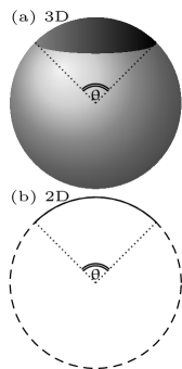
Figure 1: (a) In three dimensions (3D), given a spherical surface (shaded lighter gray), a spherical cap(sid) (shaded darker gray) is a portion of it whose any arc subtends an angle $\uptheta$. (b) In two dimensions (2D), given a circumference (discontinuous line), an arc (continuous line) is a portion of it that subtends an angle $\uptheta$.

Before complementing the investigation on systems of hard spherical caps [8] by investigating systems of hard spherical capsids with $\uptheta\in(\uppi,2\uppi]$, it has seemed opportune to dedicate the present investigation to the two–dimensionally analogous problem: The complete phase behavior of systems of hard infinitesimally–thin circular arcs in the two–dimensional Euclidean space $\mathbb{R}^{2}$ that subtend an angle $\uptheta\in[0,2\uppi]$ [Fig. 1 (b)]. This class of hard curved particles interpolates between the hard segment, corresponding to $\uptheta=0$, and the hard circle, corresponding to $\uptheta=2\uppi$; it can be divided into the sub–class of hard infinitesimally–thin minor circular arcs, from $\uptheta=0$ up to $\uptheta=\uppi$, and the sub–class of hard infinitesimally–thin major circular arcs, from $\uptheta=\uppi^{+}$ up to $\uptheta=2\uppi$ (Fig. 2).

Figure 2: Examples of circular arcs. They have the same length and different subtended angle $\uptheta$. Those in the top row are minor: (a) $\uptheta=0$; (b) $\uptheta=\displaystyle\frac{\uppi}{2}$; (c) $\uptheta=\uppi$. Those in the bottom row are major: (d) $\uptheta=\displaystyle\frac{4}{3}\uppi$; (e) $\uptheta=\displaystyle\frac{5}{3}\uppi$; (f) $\uptheta=2\uppi$.

In addition to the utility of addressing the same type of physical problem across different dimensions, there is another motivation to investigate the complete phase behavior of systems of hard infinitesimally–thin circular arcs. It is the desire of exploring whether the recently constructed densest–known packings of hard infinitesimally–thin major circular arcs [10] or sub–optimal versions of them can spontaneously form. These densest–known packings consist of compact circular clusters that comprise

$$\mathtt{n}=\left[\frac{2\uppi}{\uptheta-\uppi}\right]$$ (1)

[11] (anti)clockwise intertwining hard infinitesimally–thin major circular arcs and dispose themselves with their centres of mass at the sites of a triangular lattice [10]. It should be probed whether a similar cluster phase will finally emerge out of a competition with the other phases that systems of hard infinitesimally–thin circular arcs form.

To characterise these phases, a set of order parameters and correlation functions was considered (Section II.1). These structural descriptors were calculated by statistically analysing the configurations that were saved and stored in the course of isobaric(–isothermal) Monte Carlo numerical simulations [12; 13; 14] (Section II.2). Out of the phases that the resulting phase diagram features, one is that cluster phase. Provided $\uprho$ is sufficiently high, it forms in systems of hard infinitesimally–thin (quasi) major circular arcs. This phase constitutes the spontaneous, though sub–optimal, version of the densest–known packings that have been recently determined [10] (Section III). While sketching this phase diagram, a few traits of the phases that it features and of the transitions between them emerge. that would require as many dedicated theoretical investigations. It is hoped that the present results stimulate these theoretical investigations along with the preparation of colloidal or granular thin-circular-arc–shaped particles and the ensuing experimental investigation of systems of them (Section IV).

II methods

II.1 order parameters and correlation functions

Certain of the order parameters and correlation functions are ordinary and prefigurable based on the non-sphericity and (generally $\mathsf{D}_{{\mathrm{1}}}$ [15]) symmetry of the present hard particles and the abundant previous work on systems of hard (non-)spherical particles [2].

The most basic correlation function is the positional pair–correlation function which, in an uniform, or treated as if it were such, system of $N$ particles is usually indicated as $g(r)$. It can be defined as:

$$g(r)=\frac{1}{N}\left\langle\frac{1}{\uprho}\sum_{i=1}^{N}\sum_{j\neq i}^{N}\updelta\left(\left|{\mathbf{r}}_{j}-{\mathbf{r}}_{i}\right|-r\right)\right\rangle$$ (2)

with $\left\langle\,\right\rangle$ signifying a mean over configurations, $\updelta()$ the usual $\updelta$-function and $\mathbf{r}_{i}$ the position of the centroid of particle $i$; presently, this centroid coincides with the vertex of the circular arc $i$ (Fig. 3).

Figure 3: Example of a circular arc $i$ (continuous line), in a Cartesian $(x,y)$ reference frame with several quantities that define its mechanical state and enter the definition of order parameters and correlation functions: $\mathbf{r}_{i}$, the vector of the position of its vertex; ${\hat{\mathbf{u}}}_{i}$, the unit vector of its orientation, which lies on the direction joining the centre of its parent circle with the vertex and forms an angle $\upvarphi_{i}$ with the $x$ axis; $\mathbf{c}_{i}$, the vector of the position of the centre of its parent circle (discontinuous line) whose radius is $R$.

One order parameter that the symmetry of the present hard particles simply suggests is the polar order parameter S₁. It can be defined as:

$$\mathtt{S}_{1}=\frac{1}{N}\left\langle\left|\sum_{i=1}^{N}\mathsf{e}^{\mathsf{i}\upvarphi_{i}}\right|\right\rangle=\frac{1}{N}\left\langle\left|\sum_{i=1}^{N}{\hat{\mathbf{u}}}_{i}\right|\right\rangle\,$$ (3)

with ${\hat{\mathbf{u}}}_{i}=(\cos\upvarphi_{i}\,,\,\sin\upvarphi_{i})$ the unit vector along the symmetry axis of the circular arc $i$ (Fig. 3).

The non-sphericity of the present hard particles suggests the calculation of the nematic order parameter $\mathtt{S}_{2}$. It can be defined as:

$$\mathtt{S}_{2}=\frac{1}{N}\left\langle\left|\sum_{i=1}^{N}\mathsf{e}^{\mathsf{i}2\upvarphi_{i}}\right|\right\rangle=\left\langle\frac{1}{N}\sum_{i=1}^{N}\left[2\left({\hat{\mathbf{u}}}_{i}\cdot{\hat{\mathit{n}}}\right)^{2}-1\right]\right\rangle\,$$ (4)

with ${\hat{\mathit{n}}}$ the nematic director, i.e., the direction along which the orientation of a circular arc more probably aligns [16].

The two order parameters $\texttt{S}_{1}$ and $\texttt{S}_{2}$ would serve to establish whether and of which type a phase possesses orientational order. In actuality, associated to each of these order parameters is there an orientational pair–correlation function that provides significantly more information. The two respective correlation functions, ${\mathcal{G}}_{1}(r)$ and ${\mathcal{G}}_{2}(r)$, are defined as:

$${\mathcal{G}}_{1}(r)=\left\langle\frac{\sum_{i=1}^{N}\sum_{j\neq i}^{N}\updelta\left(\left|{\mathbf{r}}_{j}-{\mathbf{r}}_{i}\right|-r\right)\left({\hat{\mathbf{u}}}_{i}\left({\mathbf{r}}_{i}\right)\cdot{\hat{\mathbf{u}}}_{j}\left({\mathbf{r}}_{j}\right)\right)}{\sum_{i=1}^{N}\sum_{j\neq i}^{N}\updelta\left(\left|{\mathbf{r}}_{j}-{\mathbf{r}}_{i}\right|-r\right)}\right\rangle\,;$$ (5)

$${\mathcal{G}}_{2}(r)=\left\langle\frac{\sum_{i=1}^{N}\sum_{j\neq i}^{N}\updelta\left(\left|{\mathbf{r}}_{j}-{\mathbf{r}}_{i}\right|-r\right)\left(2\left({\hat{\mathbf{u}}}_{i}\left({\mathbf{r}}_{i}\right)\cdot{\hat{\mathbf{u}}}_{j}\left({\mathbf{r}}_{j}\right)\right)^{2}-1\right)}{\sum_{i=1}^{N}\sum_{j\neq i}^{N}\updelta\left(\left|{\mathbf{r}}_{j}-{\mathbf{r}}_{i}\right|-r\right)}\right\rangle\,.$$ (6)

Not only would the values of $\mathtt{S}_{1}$ and $\mathtt{S}_{2}$ be obtainable from the $r\rightarrow\infty$ limit of, respectively, ${\mathcal{G}}_{1}(r)$ and ${\mathcal{G}}_{2}(r)$ but also the calculation of orientational pair–correlation functions allows one to more profoundly characterise the orientational order of a phase. In fact, the possible tendency of two particles to mutually align can be characterised for any distance separating them and the way by which that long-distance limit is approached can be probed [17].

The possible formation of anisotropic phases suggests the definition of additional orientational pair–correlation functions whose argument is the inter-particle distance vector that is resolved along a certain specific direction. In particular, one can consider the orientational pair–correlation function ${\mathcal{G}}_{1,\perp}^{\hat{\mathbf{u}}}(r_{\perp})$ defined as:

$${\mathcal{G}}_{1,\perp}^{\hat{\mathbf{u}}}(r_{\perp})=\left\langle\frac{\sum_{i=1}^{N}\sum_{j\neq i}^{N}\updelta\left(\left|{\mathbf{r}}_{j}-{\mathbf{r}}_{i}-\left({\mathbf{r}}_{j}-{\mathbf{r}}_{i}\right)\cdot{\hat{\mathbf{u}}}_{i}{\hat{\mathbf{u}}}_{i}\right|-r_{\perp}\right)\left({\hat{\mathbf{u}}}_{i}\left({\mathbf{r}}_{i}\right)\cdot{\hat{\mathbf{u}}}_{j}\left({\mathbf{r}}_{j}\right)\right)}{\sum_{i=1}^{N}\sum_{j\neq i}^{N}\updelta\left(\left|{\mathbf{r}}_{j}-{\mathbf{r}}_{i}-\left({\mathbf{r}}_{j}-{\mathbf{r}}_{i}\right)\cdot{\hat{\mathbf{u}}}_{i}{\hat{\mathbf{u}}}_{i}\right|-r_{\perp}\right)}\right\rangle\,.$$ (7)

It probes the polar orientational correlations between two particles separated by a distance vector that is resolved along the direction perpendicular to the orientation of one of them.

The particular nature of the present hard particles and the fact that systems of them may form, in addition to the isotropic and (quasi)nematic [18] phases, distinctive phases suggest special order parameters and correlation functions.

The particular nature of the present hard particles suggests to probe the positional correlation between a pair of them in terms of the centres of their parent circles. The definition of the corresponding pair–correlation function $G(c)$ parallels that of $g(r)$ in Eq. 2:

$$G(c)=\frac{1}{N}\left\langle\frac{1}{\uprho}\sum_{i=1}^{N}\sum_{j\neq i}^{N}\updelta\left(\left|{\mathbf{c}}_{j}-{\mathbf{c}}_{i}\right|-c\right)\right\rangle$$ (8)

with ${\mathbf{c}_{i}}$ the position of the centre of the parent circle of particle $i$ (Fig. 3) [19].

In analogy with the phase behavior of hard spherical caps with $\uptheta\in[0,\pi]$ [8 (b)], systems of hard infinitesimally–thin minor circular arcs may form a filamentary phase (Fig. 4).

Figure 4: Schematic illustration of a configuration of an idealised prototypical version of the filamentary phase in a system of hard infinitesimally–thin minor circular arcs with, e.g., $\uptheta=1$.

In a filament of this phase, the hard infinitesimally–thin minor circular arcs tend to organise on the same semicircumference with the centres of the parent circles that ensuingly and randomly file; a single filament is thus polar. Different filaments of this phase may dispose themselves in a row along a direction approximately perpendicular to the filament axis, separated by a distance approximately equal to $2R$ and (anti)parallel oriented to adjacent filaments; the filamentary phase is (more probably) non-polar. If particularly preceded by a (quasi)nematic phase, the formation of this phase can be revealed by a decrease in the values of $\mathtt{S}_{2}$. More generally, its formation can be revealed by the appearance of oscillations in the ${\mathcal{G}}_{1,\perp}^{\hat{\mathbf{u}}}(r_{\perp})$ and a sequence of equi-spaced peaks in the $g(r)$ and $G(c)$.

The structure of the densest–known packings of hard infinitesimally–thin major arcs [10] suggests a suitably modified hexatic bond–orientational order parameter. These densest–known packings and the corresponding cluster hexagonal phase have a two–level structural organisation (Fig. 5).

Figure 5: Schematic illustration of a configuration of an idealised prototypical version of a cluster hexagonal phase in a system of hard infinitesimally–thin major circular arcs with, e.g., $\uptheta=1.3\uppi=4.084\cdots$. Roundish clusters of hard infinitesimally–thin major circular arcs dispose themselves with their centres of mass at the sites of a triangular lattice. The hard infinitesimally–thin major circular arcs are with, e.g., $\uptheta=1.3\uppi=4.084\cdots$ so that each roundish cluster is composed of a maximum of $\mathtt{n}=6$ of them (Eq. 1, [11]). The hard infinitesimally–thin major circular arcs are purposedly structurally organised in an expanded configuration to aid the appreciation of their (anti)clockwise “vortical” structural organisation. Towards the densest–known packings, each roundish cluster progressively contracts and the triangular–lattice spacing consequently decreases up to a point that hard infinitesimally–thin major circular arcs essentially are on the same circumference and the triangular–lattice spacing is equal to $2R$.

On the first level, a maximum of $\mathtt{n}$ (Eq. 1, [11]) hard infinitesimally–thin major circular arcs form roundish clusters that remind a vortex. On the second level, these roundish clusters organise in configurations that remind the densest configuration of hard circles [20]. This second-level structural organisation suggests a hexatic bond-orientational order parameter $\uppsi_{6}$. It is defined as

$$\uppsi_{6}=\left\langle\frac{1}{\mathcal{N}}\left|\sum_{i=1}^{\mathcal{N}}\frac{1}{{\rm{n}_{\rm vic}}_{i}}\sum_{j=1}^{{\rm{n}_{\rm vic}}_{i}}\mathsf{e}^{\mathtt{i}6\upvarphi_{ij}}\right|\right\rangle$$ (9)

with: $\mathcal{N}$ the number of roundish clusters; ${\rm{n}_{\rm vic}}_{i}$ the number of vicinal roundish clusters $j$ of a certain roundish cluster $i$, defined as those roundish clusters $j$ whose centres of mass are within a pre-fixed distance from the centre of mass of the roundish cluster $i$; $\upvarphi_{ij}$ the angle that the fictious “bond” between the roundish clusters $i$ and $j$ forms with an arbitrary fixed axis. The application of this order parameter naturally presupposes that sufficiently compact and numerous roundish clusters are at least incipient. This can be detected by $G(c)$ via a peak at $c=0$. Further growth of this peak together with the growth of the peak at $c=2R$ and the progressive split of the peak at $c\simeq 4R$ reveal that the processes of formation of roundish clusters and of their hexagonal structural organisation are consolidating.

II.2 monte carlo numerical simulations

Systems of hard infinitesimally-thin circular arcs were investigated by Monte Carlo (MC) [12; 14] method in the isobaric(–isothermal) ($NPT$) [13; 14] ensemble. The number of particles usually was $N=600$, although larger values of $N$ were also considered such as $N=5400$ for various values of $\uptheta$ and occasionally $N=6400$ in the limit $\uptheta\rightarrow 0$. The $N$ hard infinitesimally–thin circular arcs were placed in an either rectangular or parallelogrammatic variable container. The usual periodic boundary conditions were applied. The pressure $P$ was measured in units $k_{B}\,T\,\ell^{-2}$ with $k_{B}$ the Boltzmann constant, $T$ the absolute (thermodynamic) temperature and $\ell=\uptheta R$ the length of a circular arc. For any value of $\uptheta$ that was investigated, many values of the dimensionless pressure $P^{\star}=P\ell^{2}/(k_{B}T)$ were considered. For any value of these, the initial configuration was: Either a (dis)ordered configuration that was ad hoc constructed; or a configuration that was previously generated in a MC calculation at a nearby value of $\uptheta$ or $P^{\star}$. From the initial configuration, the MC calculations (sequentially) proceeded. Successive changes were attempted. Each of them was randomly chosen among $2N+1$ possibilities: With probability $N/(2N+1)$, a random translation of the centroid of a randomly selected particle; with probability $N/(2N+1)$, a random rotation of the symmetry axis of a randomly selected particle; with probability $1/(2N+1)$, a modification of one randomly selected side of the container. The (pseudo)random number generator that was employed was one that implements the Mersenne twister mt19937 algorithm [21]. These changes were accepted if no overlap resulted or rejected otherwise. The acceptance of a change in the shape and size of the container was further subject to the “Metropolis–like” criterion that characterises the MC method in the $NPT$ ensemble [13; 14]. For any specific values of $\uptheta$ and $P^{\star}$, the maximal amounts of change were adjusted so that 20–30% of each type of change could be accepted; these adjustments were carried out in the course of exploratory MC calculations; the maximal amounts of change were not altered in the course of subsequent MC calculations that were conducted at those specific values of $\uptheta$ and $P^{\star}$. To improve on the efficiency of the MC calculations, neighbour lists or linked-cell lists were employed [14 particularly (a)]. In both cases, the operative parameter was $r_{\rm cut}=4R\sin\left(\uptheta/4\right)$ which is the minimal distance at which two hard infinitesimally–thin circular arcs do not overlap irrespective of their mutual orientation. In the case of neighbour lists, the list of neighbours of a particle $i$ comprised those particles $j$ whose distance from the centroid of $i$ was smaller than $r_{\rm cut}+r_{\rm skin}$; $r_{\rm skin}$ was that distance that had been selected in the course of exploratory MC calculations as the one that provided the largest efficiency. Neighbour lists were automatically updated as soon as $[r_{\rm skin}-2{\rm d}_{\rm max}]\upkappa<r_{\rm cut}(1-\upkappa)$; d_max was the maximum among the particle displacements since the last update of the neighbour lists; $\upkappa$ was the ratio between the new and old values of the length of the modified side. In the case of linked-cell lists, generally rectangular cells were constructed whose minor side was at least equal to $r_{\rm cut}$ so that the largest possible number of cells could be obtained. Linked-cell lists were automatically updated as soon as, following a change in the side of the container: Either the minor side of a cell became smaller than $r_{\rm cut}$ and thus a smaller number of cells had to be considered; or it became sufficiently larger than $r_{\rm cut}$ to allow for more cells to be considered. For any specific values of $\uptheta$ and $P^{\star}$, exploratory MC calculations were conducted to decide which type of lists led to the largest efficiency; neighbour (linked-cell) lists were usually more efficient at higher (lower) density, where the particle mobility was relatively small (large). It was also attempted to combine neighbour lists with linked-cell lists but to no avail: Efficiency did not significantly improve with respect to separately considering the sole neighbour lists or linked-cell lists. The MC calculations were organised in cycles, each of these comprising $2N+1$ attempts of a change. For any specific values of $\uptheta$ and $P^{\star}$, the MC calculations were subdivided into an equilibration run and a production run. Usually, an equilibration run lasted $10^{7}$ cycles while the subsequent production run lasted as many cycles. In the course of the production runs, one every $10^{4}$ configurations was saved and stored for the subsequent statistical analysis. This statistical analysis comprised: The calculation of the mean number density $\left\langle\uprho\right\rangle$, $\uprho$ being measured in units $\ell^{-2}$ so that the dimensionless number density is $\uprho^{\star}=\uprho\ell^{2}$ and its mean $\left\langle\uprho^{\star}\right\rangle=\left\langle\uprho\right\rangle\ell^{2}$; the calculation of the order parameters and correlation functions that are described in Section II.1; the errors in $\left\langle\uprho^{\star}\right\rangle$ and in the order parameters were estimated by a habitual blocking method [22].

III results

III.1 description

By combining the equation of state and the set of order parameters and correlations functions (Section II.1) and with the aid of the visual inspection of configurations, four (distinctive) phases have been identified. On varying $\uprho$ and $\uptheta$, in addition to (I) a (quasi)nematic phase, systems of hard infinitesimally–thin circular arcs can form: (II) a (cluster) isotropic phase where, if $\uprho$ is sufficiently high, either filamentous or roundish clusters of hard infinitesimally–thin circular arcs are recognisable; (III) a filamentary phase as schematically depicted as in Fig. 4; (IV) a cluster hexagonal phase as schematically depicted as in Fig. 5. The regions that the four phases occupy in the $\uptheta$ versus $1/{\uprho^{\star}}$ plane, together with the curves that delimit them, configure the phase diagram in Fig. 6. In describing this phase diagram, it is convenient to subdivide it into four, $\uptheta$-dependent, sections: (i) $\displaystyle 0\leq\uptheta\lesssim\frac{\uppi}{4}$; (ii) $\displaystyle\frac{\uppi}{4}\lesssim\uptheta<\uppi$; (iii) $\uptheta\sim\uppi$; (iv) $\uptheta>\uppi$.

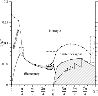
Figure 6: Phase diagram of systems of hard infinitesimally–thin circular arcs in the plane aperture angle $\uptheta$ versus inverse of dimensionless number density $1/\uprho^{\star}$. Black circles correspond to the original data that have been acquired from the MC numerical simulations while the solid lines that transverse them are guides to the eye. The gray region on the left is the co-existence region that separates the filamentary phase from either the isotropic phase or the cluster hexagonal phase. The hatched regions on the right are those regions that are effectively or theoretically prohibited as they correspond to values of number density that are higher than the values of number density of the effective or theoretical densest(–known) packings: The upper mostly monotonic curve that transverses the relevant black circles and delimits the extra region that is hatched with oblique lines from top-left to bottom-right corresponds to the effectively densest packings whose number density has been acquired from the MC numerical simulations; the lower zigzagging curve that delimits the region that is hatched with oblique lines from bottom-left to top-right corresponds to the theoretical densest–known packings [10; 11]. The two dotted lines towards the hard–circle limits indicate the two possible scenarios of the isotropic–cluster hexagonal phase transition line while approaching that limit. The three dashed rectangles enclose the most delicate regions of the phase diagram.

III.1.1 $0\displaystyle\leq\uptheta\lesssim\frac{\uppi}{4}$

The left-handed side of this section corresponds to the phase behavior of systems of hard segments. The numerical simulation data for this basic reference system were usually interpreted as inconsistent with a second–order isotropic–nematic phase transition that the application of a second–virial (Onsager [23]) density functional theory would predict [24]. They were usually interpreted as consistent with the existence of an isotropic–(quasi)nematic phase transition of the Berezinskii–Kosterlitz-Thouless [25; 26; 27; 28] type [29; 30; 31]. One interpretation that essentially maintains both of these two, usually mutually exclusive, interpretations was also proposed [32]. In an infinite periodic system, the S-shaped curve of $\mathtt{S}_{2}$ versus $\uprho$ is suggestive of an isotropic–nematic phase transition. In three dimensions, it would be indeed taken as a signature of such a phase transition. In two dimensions, it is instead considered insufficient. This insufficiency is based on assuming that basic analytic results for specific two–dimensional systems [33; 34] have to also preclude a proper long–ranged nematic ordering in a two-dimensional system. Even though those analytic results were found inapplicable to a two-dimensional nematic phase that is formed in a realistic system of particles interacting via non–separable interactions as hard particles are [35]. Based on that paradigm, $\mathtt{S}_{2}$ of an infinite (thermodynamic) system would be equal to zero at all values of $\uprho$. For this reason, one should turn to explicitly considering ${\mathcal{G}}_{2}(r)$ and its long-distance behavior. The latter distinguishes the two phases at either side of a phase transition of the Berezinskii–Kosterlitz-Thouless type: In the isotropic phase, ${\mathcal{G}}_{2}(r)$ decays to zero exponentially; in the (quasi)nematic phase, ${\mathcal{G}}_{2}(r)$ decays to zero algebraically. Even though past and present numerical simulation data seem to be consistent with this scenario, the limited size of the systems that are considered in these numerical simulations cannot afford to clearly and unambiguously discern the characteristics of the long-distance decay. It is difficult to extrapolate to a very long distance the behavior of a correlation function that is known up to a decade of distance units. Based on this modest distance interval, it is difficult to affirm what is the best fitting function overall. It seems that, for sufficiently large values of $\uprho$, an algebraic fitting function outperforms an exponential fitting function. However, other fitting functions could perform even better: e.g., a “stretched-exponential” function fares at least as well as an algebraic function.

Based on these considerations, the attitude of this work is very pragmatic. In analogy to previous works [29; 30], ${\mathcal{G}}_{2}(r)$ has been fitted to either an exponential or algebraic function. The value of $\uprho$ at which the latter fitting function seems to outperform the former fitting function is taken as the value that delimits the isotropic phase and the (quasi)nematic phase. This is done without claiming it as objectively supporting a phase transition of the Berezinskii–Kosterlitz-Thouless type while conceding the present impossibility to more profoundly investigate the nature of the two-dimensional nematic phase and of the transition that separates it from the isotropic phase.

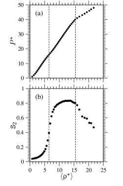
Figure 7: (a) equation of state $P^{\star}$ versus $\langle\uprho^{\star}\rangle$ and (b) nematic order parameter $\mathtt{S}_{2}$ versus $\langle\uprho^{\star}\rangle$ for a system of hard infinitesimally–thin circular arcs with $\uptheta=0.5$. The dashed vertical line on the left separates the isotropic phase and the (quasi)nematic phase while the dashed vertical line on the right separates the (quasi)nematic phase and the filamentary phase.

In a system of hard infinitesimally–thin minor circular arcs with $\uptheta=0.25$, the isotropic and (quasi)nematic phases are the sole phases that have been observed in the interval of values of $P$ that has been presently investigated. Hard infinitesimally–thin minor circular arcs with $\uptheta=0.5$ are instead sufficiently curved for another, denser and arguably more interesting, phase to succeed the (quasi)nematic phase already in the interval of values of $P$ that has been presently investigated. This phase transition is revealed by a bent in the equation of state and a descent in the values of $\mathtt{S}_{2}$ (Fig. 7). These two signs are accompanied by a significant change in the long-distance behavior of ${\mathcal{G}}_{2}(r)$: On going from the lower-density phase to the higher-density phase, the long-distance behavior of ${\mathcal{G}}_{2}(r)$ seems as if it revert to that in the isotropic phase: No remnant of a possible algebraic decay remains [Fig. 8 (a)]. One appreciates that the phase that spontaneously forms at larger values of $\uprho$ is the filamentary phase [Fig. 8 (b, c, d)]. In fact, this phase is characterised by hard infinitesimally–thin minor circular arcs tending to organise on the same semicircumference; in turn, these generated semicircular clusters file to generate filaments; in turn, these filaments tend to mutually organise side-by-side and up-side-down [Fig. 8 (d)]. Consistently, ${\mathcal{G}}_{1,\perp}^{\hat{\mathbf{u}}}(r_{\perp})$ exhibits a short-distance oscillatory behavior with a period approximately equal to $2R$ [Fig. 8 (e)].

Figure 8: (a) The orientational pair–correlation function ${\mathcal{G}}_{2}(r)$ in the isotropic phase at $P^{\star}=10$ (dotted line), (quasi)nematic phase at $P^{\star}=35$ (dashed line) and filamentary phase at $P^{\star}=45$ (solid line). Image of a configuration in the (b) isotropic phase at $P^{\star}=10$, (c) (quasi)nematic phase at $P^{\star}=35$ and (d) filamentary phase at $P^{\star}=45$. (e) The orientational pair–correlation function ${\mathcal{G}}_{1,\perp}^{\hat{\mathbf{u}}}(r_{\perp})$ in the isotropic phase at $P^{\star}=10$ (dotted line), (quasi)nematic phase at $P^{\star}=35$ (dashed line) and filamentary phase at $P^{\star}=45$ (solid line).

It is conceivable that the filamentary phase also forms in systems of hard infinitesimally–thin minor circular arcs with $\uptheta<0.5$ at increasingly higher density and pressure than those that have been presently investigated.

By the concomitant action of both the isotropic phase at lower $\uprho$ and the filamentary phase at higher $\uprho$, the number density interval in which the (quasi)nematic phase exists precipitously contracts as $\uptheta$ increases until this phase disappears at $\displaystyle\uptheta\simeq\frac{\uppi}{4}$.

III.1.2 $\displaystyle\frac{\uppi}{4}\lesssim\uptheta<\uppi$

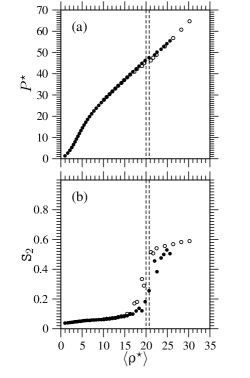
Figure 9: (a) equation of state $P^{\star}$ versus $\langle\uprho^{\star}\rangle$ and (b) nematic order parameter $\mathtt{S}_{2}$ versus $\langle\uprho^{\star}\rangle$ for a system of hard infinitesimally–thin circular arcs with $\uptheta=1.8$. In both panels, filled circles correspond to data that were obtained by progressively compressing the system from an initial dilute and disordered configuration while empty circles correspond to data that were obtained by progressively decompressing the system from an initial filamentary configuration as that schematically depicted as in Fig. 4. The two dashed vertical lines separate the isotropic phase and the filamentary phase.

In this section, the isotropic and filamentary are the sole phases that have been observed. These two phases are separated by a first-order phase transition whose strength increases with increasing $\uptheta$. This is revealed by the behavior of the equation of state [Fig. 9 (a)]. $\mathtt{S}_{2}$ concurs to reveal this phase transition: $\mathtt{S}_{2}$ exhibits a surge in correspondence to the values of $\uprho$ at which the phase transition occurs; the values that this order parameter takes on in the filamentary phase are significantly smaller than those typical of a (quasi)nematic phase [Fig. 9 (b)]. In fact, in an idealised prototypical filamentary phase as schematically depicted as in Fig. 4, the $\mathtt{S}_{2}$ would take on a value equal to $\displaystyle\frac{\sin(\uptheta-\uppi)}{\uptheta-\uppi}$. The structural differences that occur on going from the isotropic phase to the filamentary phase are revealed by the various pair–correlation functions (Fig. 10). Particularly, $G(c)$ becomes to peak at $c=2R$ and $c=4R$ [cf. (a) and (b) in Fig. 10], while ${\mathcal{G}}_{1,\perp}^{\hat{\mathbf{u}}}(r_{\perp})$ becomes oscillatory with a period equal to $4R$ [cf. (e) and (f) in Fig. 10]. On increasing $\uptheta$, as the transition to the filamentary phase is approached, the isotropic phase passes from being ordinary to exhibiting clusters. These clusters are made of hard infinitesimally–thin circular arcs that tend to organise on the same semicircumference and then file to generate filaments that are of varying length, degree of ramification and tortuousity [inset in Fig. 10 (c)]. The progressive straightening of the equation of state is a symptom of the formation of these “supraparticular” structures that precurse a proper filamentary phase. On increasing $\uptheta$, in the same filamentary phase, the filaments tend to be more tortuous and it is increasingly more frequent to observe ramifications and “ruptures”. These ramifications and “ruptures” are provoked by hard infinitesimally–thin circular arcs that tend to dispose in an antiparallel configuration [inset in Fig. 10 (d)].

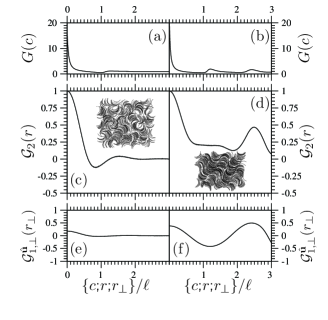
Figure 10: For a system of hard infinitesimally–thin circular arcs with $\uptheta=1.8$ in the isotropic phase at $P^{\star}=40$ and in the filamentary phase at $P^{\star}=53$, the positional pair-correlation function $G(c)$ (a and b, respectively), the orientational pair-correlation function ${\mathcal{G}}_{2}(r)$ (c and d, respectively) and the orientational pair-correlation function ${\mathcal{G}}_{1,\perp}^{\hat{\mathbf{u}}}(r_{\perp})$ (e and f, respectively) are shown. The inset in (c) is an image of a configuration in the isotropic phase at $P^{\star}=40$ while the inset in (d) is an image of a configuration in the filamentary phase at $P^{\star}=53$.

III.1.3 $\uptheta\sim\uppi$

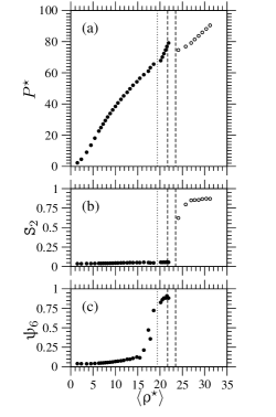
Figure 11: (a) equation of state $P^{\star}$ versus $\langle\uprho^{\star}\rangle$, (b) nematic order parameter $\mathtt{S}_{2}$ versus $\langle\uprho^{\star}\rangle$ and (c) hexatic order parameter $\uppsi_{6}$ versus $\langle\uprho^{\star}\rangle$ for a system of hard infinitesimally–thin circular arcs with $\uptheta=3$. In panels (a) and (b) filled circles correspond to data that were obtained by progressively compressing the system from an initial dilute and disordered configuration while empty circles correspond to data that were obtained by progressively decompressing the system from an initial filamentary configuration as that schematically depicted as in Fig. 4. In the three panels, the vertical dotted line separates the isotropic phase and the cluster hexagonal phase while the two vertical dashed lines separate the cluster hexagonal phase and the filamentary phase.

In this section, a new, arguably most interesting, phase appears in between the isotropic phase and the filamentary phase: The cluster hexagonal phase. In the isotropic phase, the tendency that filamentous clusters have to break and close up increases up to conducing to the formation of roundish clusters. This occurs up to a point that the roundish clusters become sufficiently compact and numerous and their number sufficiently large to organise in a triangular lattice. The formation of this cluster hexagonal phase, which prevents the spontaneous formation of the filamentary phase, can be revealed by examining the equation of state: It corresponds to a tenuous surge in its graph that is recognisable at values of $\uprho^{\star}\simeq 20$ [Fig. 11 (a)]. While $\mathtt{S}_{2}$ is unable to reveal this phase transition [Fig. 11 (b)], better evidence of a transition between the isotropic phase and the cluster hexagonal phase is nonetheless acquired by examining the dependence of $\uppsi_{6}$ on $\uprho$: This order parameter exhibits a clear surge in correspondence to the isotropic–cluster hexagonal phase transition [Fig. 11 (c)]. $\mathtt{S}_{2}$ can instead distinguish between the cluster hexagonal phase and the filamentary phase: Since the roundish clusters are overall isotropic, $\mathtt{S}_{2}$ (effectively) vanishes in the cluster hexagonal phase as it does in the isotropic phase; since the structural units of the filamentary phase are formed by a progressively smaller number of hard infinitesimally–thin minor circular arcs as $\uptheta\rightarrow\uppi$, $\mathtt{S}_{2}$ is increasingly significantly larger than zero in the filamentary phase [Fig. 11 (b)]. The two cluster phases are separated by a first–order phase transition.

Figure 12: For a system of hard infinitesimally–thin circular arcs with $\uptheta=3$ in the isotropic phase at $P^{\star}=25$, the cluster hexagonal phase at $P^{\star}=34$ and the filamentary phase at $P^{\star}=34$: (a) the positional pair–correlation function $g(r)$; (b) the positional pair–correlation function $G(c)$; (c, d, e) image of a configuration respectively in the isotropic phase, cluster hexagonal phase and filamentary phase; (f) the orientational pair–correlation function ${\mathcal{G}}_{1}(r)$; (g) the orientational pair–correlation function ${\mathcal{G}}_{2}(r)$; (h) the orientational pair–correlation function ${\mathcal{G}}_{1,\perp}^{\hat{\mathbf{u}}}(r_{\perp})$; in panel (a, b, f, g, h), the dotted, solid and dashed lines are respectively for the isotropic, cluster hexagonal and filamentary phases.

The structural differences among the three phases are revealed by the various pair–correlation functions and evidenced by the corresponding images of a configuration (Fig. 12). Based on these images, one notes the similarity between the structures of the isotropic phase and of the cluster hexagonal phase which contrast with the structure of the filamentary phase. This (dis)similarity among the three phases is reflected in the graphs of the various pair–correlation functions (Fig. 12).

III.1.4 $\uptheta>\uppi$

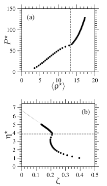
Figure 13: equation of state (a) in the representation $P^{\star}$ versus $\langle\uprho^{\star}\rangle$ and (b) in the representation $\upeta^{\star}$ versus $\upzeta$ for a system of hard infinitesimally–thin circular arcs with $\uptheta=1.1\uppi=3.455\cdots$; in (a) the vertical dashed line and in (b) the horizontal dashed line separates the isotropic phase and the cluster hexagonal phase; in (b) the dotted line is a linear fit extrapolation of the higher-density part of the solid-phase branch.

The fact that $\uptheta$ surpasses the intermediate value of $\uppi$ is very consequential. It was already observed that two hard infinitesimally–thin major circular arcs that are disposed on top of one another cannot superpose; they can only superpose if they are suitably rotated with respect to one another in a way that, once it is exactly replicated $\mathtt{n}$ (Eq. 1, [11]) - 2 times, conduces to the formation of those compact circular clusters that characterise the corresponding densest–known packings [10]. This fact significantly destabilises the filamentary phase with respect to the cluster hexagonal phase: The former phase precipitously disappears leaving the latter phase as the sole observable phase at sufficiently high $\uprho$. The cluster hexagonal phase is separated from the isotropic phase by a transition whose weakness presently makes impossible to assess whether it is either (more probably) first-order or second-order. This phase transition is revealed by a visually recognisable change in the graph of the equation of state [Fig. 13 (a)]. This change may be made clearer by plotting the effective packing fraction $\displaystyle\upeta^{\star}=\frac{\uprho\uppi R^{2}}{\uppi/(2\sqrt{3})}$ with respect to the inverse compressibility factor $\upzeta=\displaystyle\frac{\uprho^{\star}}{P^{\star}}$ [Fig. 13 (b)]. One further revealer of the formation of a cluster hexagonal phase is again $\uppsi_{6}$: It exhibits a surge in correspondence to $\langle\uprho^{\star}\rangle\simeq 12$, the value of $\langle\uprho^{\star}\rangle$ at which the isotropic–cluster-hexagonal phase transition occurs [Fig. 14 (a)]. In addition, the form of $g(r)$ and $G(c)$ passes from being fluid–like [Fig. 14 (b, c)] to being crystalline–like [Fig. 14 (d, e)].

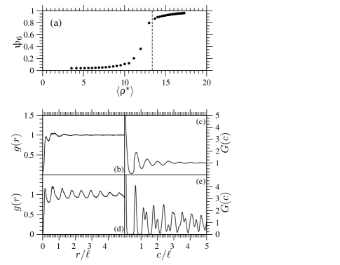
Figure 14: For a system of hard infinitesimally–thin circular arcs with $\uptheta=1.1\uppi=3.455\cdots$: (a) the order parameter $\uppsi_{6}$ as a function of number density $\langle\uprho^{\star}\rangle$; the vertical dashed line separates the isotropic phase and the cluster hexagonal phase; the pair–correlation functions $g(r)$ and $G(c)$ in the isotropic phase at $P^{\star}=56.7$ (b, c) and in the cluster hexagonal phase at $P^{\star}=128.4$ (d, e).

In the graphical representation of Fig. 13(b), one can observe that the cluster-hexagonal-phase branch is, to a good approximation, linear. This is consistent with the applicability, also to the present case, of a suitably adapted version of the free–volume theory [36]. This theory is known to provide a good (the) description and interpretation of the equation of state of a dense solid phase in a system of hard particles [36; 37]. In an equilibrium system of hard circles (discs), the linear extrapolation of the high-density solid-branch curve would intersect the ordinate axis at a value equal to 1. The linear extrapolation of the high-density solid-branch curve in a system of hard infinitesimally–thin major circular arcs with $\uptheta=1.1\uppi=3.455\cdots$ intersects the ordinate axis at a value approximately equal to 6.5 [Fig. 13 (b)]. This value corresponds to the mean value $\langle n\rangle$ of the hard infinitesimally–thin major circular arcs with $\uptheta=1.1\uppi=3.455\cdots$ per roundish cluster. This is confirmed by a more direct calculation of $\langle n\rangle$. It ensues from the calculation of the probability distribution, $\mathcal{P}$, of the number, $n$, of hard infinitesimally–thin major circular arcs per roundish cluster: ${\mathcal{P}}(n)$ [Fig. 15 (a)]. The value of $\langle n\rangle$ increases with $\langle\uprho^{\star}\rangle$ in the isotropic phase until it flatly levels up as the system enters the cluster hexagonal phase [Fig. 15 (b)]. The limit value $\langle n\rangle\simeq 6.5$ in the cluster hexagonal phase is smaller than ${\mathtt{n}}=19$ (Eq. 1, [11]) [10]. This means that the cluster hexagonal phase that spontaneously forms from the isotropic phase is a sub–optimal version of these densest–known packings. This is comprehensible as the phase transition occurs at a value of $\langle\uprho^{\star}\rangle\simeq 12$ that is still relatively small [Fig. 15 (b)]. Yet, the subsequent constancy of $\langle n\rangle$ with $\langle\uprho^{\star}\rangle$ [Fig. 15 (b)] raises two questions as to whether the densest–known packings could ever spontaneously form on progressive compression and whether the cluster hexagonal phase that spontaneously forms from the isotropic phase could ever be an equilibrium phase.

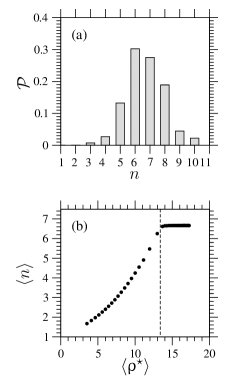
Figure 15: (a) Probability distribution function $\mathcal{P}$ of the number $n$ of hard infinitesimally–thin circular arcs per roundish cluster for a system of hard infinitesimally–thin circular arcs with $\uptheta=1.1\uppi=3.455\cdots$ at $P^{\star}=128.4$. (b) The mean value $\langle n\rangle$ of the number of hard infinitesimally–thin circular arcs per roundish cluster as a function of $\langle\uprho^{\star}\rangle$ for a system of hard infinitesimally–thin circular arcs with $\uptheta=1.1\uppi=3.455\cdots$; the vertical dashed line separates the isotropic phase and the cluster hexagonal phase.

The importance and relevance of these questions also emerge from investigating systems of hard infinitesimally–thin major circular arcs with a larger value of $\uptheta$. In these cases, more than one cluster hexagonal phase branches can be observed; these are separated by what would seem as a first–order phase transition [Fig. 16 (a)]. Such a discontinuous phase behavior can be also appreciated by examining the evolution of $\uprho^{\star}$ in the course of a Monte Carlo numerical simulation: An abrupt jump in the values of $\uprho^{\star}$ is frequently observed [Fig. 16 (b)]. This is due to the roundish clusters that are progressively re-organising in such a way that they incorporate, on the average, more constituting hard infinitesimally–thin circular arcs: In correspondence to the rise in the values of $\uprho^{\star}$ there is a momentary fall in the values of $\uppsi_{6}$; this suggests a momentary re-organisation of the system that allows the incorporation of more hard infinitesimally–thin circular arcs into the same roundish cluster(s) [Fig. 16 (c)]. The lower-density branch directly forms from the isotropic phase [Fig. 16 (a)]. If pressure is sufficiently high, then it transforms into the higher-density branch after many MC cycles (Fig. 16). From that value of pressure, the higher-density branch can be continued up to higher pressure and down to lower pressure [Fig. 16 (a)]. One may assess the lower-density branch in Fig. 16 (a) as an enduring metastable branch. However, the same assessment is applicable to the unique branch that is observed in Fig. 13 and to the higher-density branch in Fig. 16 (a) with respect to other, hypothesisable, even higher-density branches that insufficiently lengthy MC numerical simulations prevent from observing. Continuous incorporation and release of hard infinitesimally–thin circular arcs into or from roundish clusters are necessary to spontaneously attain and maintain an equilibrium ${\mathcal{P}}(n)$. In a cluster hexagonal phase, it is conceivable that the mechanisms of incorporation and release become increasingly less effective as $\uprho$ increases. Based on Figs. 13, 15, 16, it is presently unclear how an equilibrium cluster hexagonal phase should proceed towards the densest–known packing limit: Either continuously, via a gradual modification of ${\mathcal{P}}(n)$; or discontinuously, via a sequence of iso–structural first–order phase transitions, each phase at either side of the phase transition being a cluster hexagonal phase with its own ${\mathcal{P}}(n)$. The discontinuous behavior that is observed may well be an artificial effect due to the finite size of the systems that are considered in the MC numerical simulations which is further exacerbated by an (always looming) insufficiency of their duration.

On progressive compression from the isotropic phase, the capability of hard infinitesimally–thin major circular arcs of intertwining in roundish clusters persists up to values of $\uptheta$ almost equal to $2\uppi$: For a value of $\uptheta$ as large as $1.9\uppi=5.969\cdots$ a vast majority of dimers are observed. This capability should deteriorate as the value of $\uptheta$ is further increased: in the very close neighbourhood of $\uptheta=2\uppi$, a more even mixture of monomers and dimers is expected, with the former progressively becoming more abundant as the hard-circle limit is approached. In the hard-circle limit, the system is clearly formed by single hard circles. However, it is probable that this limit should be considered as a singular limit. This hypothesis relies on the densest–known packings being formed by dimers that dispose themselves at the sites of a triangular lattice for any value of $\uptheta<2\uppi$ [10]. In the thermodynamic limit at very high density, the stablest structures should correspond to these densest–known packings for any value of $\uptheta<2\uppi$ [10].

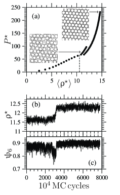
Figure 16: For a system of hard infinitesimally–thin circular arcs with $\uptheta=1.4\uppi=4.398\cdots$: (a) equation of state $P^{\star}$ versus $\langle\uprho^{\star}\rangle$; note that there are two cluster-hexagonal branches; the vertical dashed line separates the isotropic phase and the lower-density cluster-hexagonal phase; the inset on the bottom left is an image of a configuration taken at $P^{\star}=77.4$ in the lower-density cluster-hexagonal branch; the inset on the top right is an image of a configuration taken at $P^{\star}=232.1$ in the higher-density cluster-hexagonal branch; (b) evolution of the number density $\uprho^{\star}$ at $P^{\star}=77.4$ as a function of MC cycles; (c) evolution of the number density $\uppsi_{6}$ at $P^{\star}=77.4$ as a function of MC cycles.

III.2 discussion

In discussing the phase diagram that has been described, there are several comparisons to be made and connections to be established with previous works.

Section (i) resembles the phase diagram of a generalised planar rotor spin system on a square lattice. In this system, the interaction of a spin $i$ with its nearest neighbour spin $j$ comprises the (ferromagnetic or) polar term, proportional to $\cos\left(\upvarphi_{j}-\upvarphi_{i}\right)$, and the (generalised) nematic term, proportional to $\cos\left(q\left(\upvarphi_{j}-\upvarphi_{i}\right)\right)$, with $q=\rm{2,3,4}$ [38; 39; 40; 41]. This resemblance is made once the low-density isotropic (high-density filamentary) phase in the present off–lattice systems is associated to the high-temperature paramagnetic (low-temperature ferromagnetic) phase in those on–lattice systems. In both types of systems, a (quasi)nematic phase exists in between the other two respective phases. Its stability interval diminishes as, respectively, either $\uptheta$ increases or the polar term proportional to $\cos\left(\upvarphi_{j}-\upvarphi_{i}\right)$ prevails. However, this resemblance may be solely qualitative and a possible correspondence between the two types of systems may immediately end. Even though sharing the same rotational symmetry, investigations on on–lattice systems of spins interacting with a potential energy $\rm U$ of the form

$${\rm U}=-a_{1}\cos(\upvarphi_{j}-\upvarphi_{i})-a_{q}\cos\left(q(\upvarphi_{j}-\upvarphi_{i})\right)$$

with $q\geq 2$ have shown that the resulting phase diagrams can significantly depend on $q$ [40]. It is presumable that the same conclusion hold when other, more general, expressions for the potential energy of the form

$${\rm U}=-\sum_{q\geq 1}a_{q}\cos\left(q(\upvarphi_{j}-\upvarphi_{i})\right)$$

were considered [42]. The excluded area could be considered as the quantity in a two–dimensional off–lattice non–thermal model that plays a role analogous to the potential energy in a two–dimensional on–lattice thermal model. In fact, there has been an investigation of a system of spins on a square lattice interacting with a potential energy of the same form as the excluded area between two discorectangles [43]. If one adapted this exercise to the present case, one would have to calculate the excluded area between two hard infinitesimally–thin minor circular arcs. The first four terms of the Fourier series expansion of this excluded area (Table 1) would indicate that the effect of progressively curving hard segments into hard infinitesimally–thin minor circular arcs would be to generally make the effective interactions more isotropic.

$\uptheta$	$a_{1}/a_{2}$	$a_{2}/a_{2}$	$a_{3}/a_{2}$	$a_{4}/a_{2}$
0	0	1	0	0.2
0.11285	-0.000762	1	-0.000754	0.198
0.56608	-0.0214	1	-0.0196	0.158
1.14391	-0.107	1	-0.0755	0.0873

Table 1: the first four coefficients of the Fourier series of the excluded area between two hard infinitesimally–thin circular arcs that subtend an angle $\uptheta$; note that the coefficients are in units of the coefficient $a_{2}$.

These effective interactions would be essentially classifiable as a composition of an (antiferromagnetic or) antipolar term with a nematic term (Table 1). This would not be entirely compatible with the observation of a filamentary phase which, although globally non-polar, is locally polar. The passage from an on–lattice model to an off–lattice model does not seem to be that straightforward: If even maintaining the particles constrained on a lattice and changing a sole term proportional to $\cos\left(q(\upvarphi_{j}-\upvarphi_{i})\right)$ produces qualitatively different phase diagrams, then results that may be valid for an on–lattice system may not apply, especially in low dimensions, to a supposedly related off–lattice system. Not only are the centroids of the hard infinitesimally–thin circular arcs not constrained on a lattice but the interaction between two of them is also non–separable. This significantly adds to debilitating a possible association between the filamentary phase in a system of hard infinitesimally-thin minor circular arcs and the ferromagnetic phase in a system of generalised planar rotor spins: In fact, even leaving aside the positional structure of the filamentary phase, its orientational pair–correlation functions are significantly more complicated than the simple algebraically and monotonically decaying pair–correlation functions in the ferromagnetic phase.

The filamentary phase is the same phase that was observed in numerical simulations on systems of hard bow–shaped particles formed by three suitably disposed hard segments [44 (a)]. In that work, this phase was denoted as “modulated nematic” phase. In a subsequent work that attempted to reproduce these numerical simulation data with second-virial (Onsager [23]) density-functional theory analytic calculations, this phase was interpreted as a “splay–bend nematic” phase [44 (b)]. Irrespective of whether it could be qualified as generically “modulated” or particularly “splay–bend”, it is actually the application of the adjective “nematic” to this phase that does not convince. One constitutive feature of a nematic phase is its positional uniformity. The filamentary phase, even in those versions that are very rippled with ramifications, ruptures and tortuousity, is not positionally uniform: e.g., the probability density to find a particle intra-filament is not the same as that to find a particle inter-filament. One more constitutive feature of a nematic phase is its fluidity. One would expect that particles travel along the “modulation” in a “modulated” nematic phase as fast as they do along the nematic director in an ordinary nematic phase. This is what happens in the screw–like nematic phase that forms in systems of helical particles [45]. Preliminary results on the mechanism of diffusion in the filamentary phase that forms in systems of hard infinitesimally–thin circular arcs point that this is not the case [46]: Hard infinitesimally–thin circular arcs intrude from one into an adjacent filament in a step-like manner while retaining their orientation and rapidly return to the original filament or advance to the subsequent filament: A mechanism of diffusion that reminds the one operative in a smectic A phase [47]. These considerations are consistent with what has been ultimately observed in systems of hard arched particles in three dimensions. Initially, numerical simulations and experiments on systems of hard or colloidal arched particles have claimed that these systems form a splay-bend nematic phase [48 (a,b)]. Subsequently, this conclusion has been rectified: That “modulated” phase is not positionally uniform: it is not nematic but smectic-like [48 (c)].

Rather, the concavity and polarity of the present hard particles induces the recognition of another resemblance: between the cluster isotropic phase and the filamentary phase that are observed in section (ii) of the present phase diagram and the “living polymeric” phase that was observed in systems of dipolar hard circles (discs) [49]. In both present and previous systems, filaments or chains form which are tortuous and occasionally ramificates and closes up to produce roundish clusters or irregular rings.

Sections (i) and (ii) of the phase diagram of systems of hard infinitesimally–thin circular arcs constitute (nothing else than) the two–dimensional version of the phase diagram of systems of hard spherical caps with subtended angle $\uptheta\in[0,\uppi]$ [8]. In particular, the present filamentary phase is (nothing else than) the two–dimensional version of that cluster columnar phase that was observed in three–dimensional systems of hard spherical caps. Consistently to its lower dimension, the filamentary phase is subject to stronger fluctuations that should conduce to a more extensive tortuosity as well as to more ramifications and “ruptures”. Yet, the same auto-assembly phenomenology is essentially observed in both two and three dimensions. In particular, it causes the isotropic phase exhibit, at sufficiently high $\uprho$, the formation of clusters that progressively pass from being filamentous or lacy to being roundish or globular as $\uptheta$ increases. The principal difference between what is observed in two dimensions and what is observed in three dimensions is the capability of the two–dimensional roundish clusters to organise in a triangular lattice: i.e., the formation of a cluster hexagonal phase in two dimensions.

Though already incipient in section (iii), this cluster hexagonal phase completely characterises section (iv) of the phase diagram of Fig. 6. Consistently to the recent determination of the corresponding densest–known packings [10], it constitutes the truly novel phase that is observed in the present work. It forms in two dimensions while in three dimensions an analogous phase has not been observed and will probably be not observable. It forms due to the capability that hard infinitesimally–thin, particularly major, circular arcs have to intertwine without intersecting. This capability cannot be retained on going from two to three dimensions.

Similarly to what has been already commented apropos the phase behavior of systems of hard spherical caps [8], the auto-assembly phenomenology that is observed in systems of hard infinitesimally–thin circular arcs resembles what is observed in molecular systems that form micelles [50; 51]: These supramolecular structural units can be cylindrical or globular which can then auto-assemble to form a variety of complex phases among which are columnar and crystalline phases [50; 51]. There, at the origin of the complex phase behavior are complex molecules that interact between them via complicated attractive and repulsive intermolecular interactions. Here, this complex phase behavior occurs in systems of relatively simple hard particles and thus is purely entropy–driven.

IV conclusion and perspective

This work consists in an investigation on the phase behavior of systems of hard infinitesimally–thin circular arcs in the two–dimensional Euclidean space $\mathbb{R}^{2}$. Depending on the subtended angle $\uptheta$ and the number density $\uprho$, several purely entropy-driven phases are observed in the course of Monte Carlo numerical simulations [12; 13; 14].

Leaving aside the (quasi)nematic phase that is solely observed for sufficiently small values of $\uptheta$ and at intermediate values of $\uprho$, more interesting are the other phases that are observed. The very same isotropic phase is such: Provided $\uprho$ is sufficiently high, it becomes no ordinary in that it exhibits clusters which pass from being filamentous to being roundish as $\uptheta$ progressively increases. Provided $\uprho$ is even higher, these two types of clusters respectively produce a filamentary phase for $\uptheta\lesssim\uppi$ and a hexagonal phase for $\uptheta\gtrsim\uppi$. Both these phases are characterised by a “supraparticular” structural organisation: the actual structural units are formed by a number of suitably disposed hard particles. Particularly interesting is the cluster hexagonal phase. It offers examples of (soft) porous crystalloid materials [52; 53] whose porosity could be regulated by compression. The auto–assembly phenomenology in systems of hard infinitesimally–thin circular arcs, as well as that in systems of hard spherical caps [8], interestingly resemble that that occurs in micellising molecular systems [50; 51].

Despite the extensive Monte Carlo numerical simulations, there are several issues that still necessitate a clarification. Leaving aside the persistent issue of the nature of the nematic phase in a realistic two–dimensional system [35], it is the structure of the three cluster phases that would require a more detailed characterisation. This should centre on a detailed statistical analysis of the shape and size of respective clusters. Specifically in systems of hard infinitesimally–thin minor circular arcs, it should address the persistence length of the filaments and the number of their ramifications and “ruptures” [54]. Specifically in systems of hard infinitesimally–thin major circular arcs, it should ascertain whether, on progressive compression, a single hexagonal phase forms or multiple hexagonal phases form in the (long) way towards the corresponding densest–known packings [10]. The clarification of these pending issues necessitates to consider systems of a significantly larger size and improved computational resources and techniques than those presently available. Under these conditions, it would be very beneficial to have an experimental system, either colloidal or granular, of thin-circular-arc–shaped particles [55]. It could be used to first test the present predictions on the complete phase behavior and then address and aid to resolve those pending issues.

References

- [1] e.g. P. M. Chaikin and T. C. Lubensky, Principles of Condensed Matter Physics, Cambridge University Press, Cambridge (1995).
- [2] e.g. S. Torquato, J. Chem. Phys. 149, 020901 (2018).
- [3] e.g. The Plastically Crystalline State: Orientationally–Disordered Crystals, edited by J. N. Sherwood, Wiley, Chichester (1979).
- [4] e.g. L. M. Blinov, Structure and Properties of Liquid Crystals, Springer, Dordrecht (2011).
- [5] L. Mederos, E. Velasco, Y. Martínez-Ratón, J. Phys. Cond. Matter 26, 463101 (2014).
- [6] M. P. Allen, Mol. Phys. 117, 2391 (2019).
- [7] e.g. C. Avendaño and F. A. Escobedo, Curr. Op. Coll. Interface Sci. 30, 62 (2017).
- [8] (a) G. Cinacchi and J. S. van Duijneveldt, J. Phys. Chem. Lett. 1, 787 (2010); (b) G. Cinacchi, J. Chem. Phys. 139, 124908 (2013); (c) G. Cinacchi and A. Tani, J. Chem. Phys. 141, 154901 (2014).
- [9] (a) S. Sacanna, M. Korpics, K. Rodriguez, L. Colón-Meléndez, S. -H. Kim, D. J. Pine, and G. -R. Yi, Nature Comms. 4, 1688 (2013); (b) K. V. Edmond, T. W. P. Jacobson, J. S. Oh, G. -R. Yi, A. D. Hollingsworth, S. Sacanna and D. J. Pine, Soft Matter 17, 6176 (2021).
- [10] J. P. Ramírez González and G. Cinacchi, Phys. Rev. E 102, 042903 (2020).
- [11] indicates the strict floor function of the real variable . The adjective strict is used to signify that this floor function returns and not for while it behaves as an ordinary floor function for .
- [12] N. Metropolis, A. W. Rosenbluth, M. N. Rosenbluth, A. N. Teller, and E. Teller, J. Chem. Phys 21 , 1087 (1953).
- [13] W. W. Wood, J. Chem. Phys. 48, 415 (1968); ibidem 52, 729 (1970).
- [14] e.g. (a) M. P. Allen and D. J. Tildesley, Computer Simulation of Liquids, Clarendon Press, Oxford (1987); (b) W. Krauth, Statistical Mechanics: Algorithms and Computations, Oxford University Press, Oxford (2006).
- [15] Except for , in which case it is .
- [16] J. Vieillard-Baron, Mol. Phys. 28, 809 (1974). This work actually introduced the method, based on ordinary linear algebra, to calculate and for a system of hard non-spherical particles in three dimensions. The method is, mutatis mutandis, the same in a system of hard non–circular particles in two dimensions.
- [17] Higher–order orientational pair–correlation functions and their associated order parameters could be considered but, based on the experience that was acquired with systems of hard spherical caps [8], those of order one and two were considered sufficient. In addition, more general orientational pair–correlation functions that depend not only on the modulus but also on the direction of the inter–particle distance vector could be profitably considered.
- [18] The pre-fix (quasi) is added to indicate that, in a two–dimensional system, a proper long-ranged nematic ordering, like any other proper long-ranged ordering, would not exist.
- [19] Orientational pair–correlation functions similar to Eqs. 5 and 6 could be defined in terms of the centres of the parent circles but their calculation was omitted.
- [20] e.g., P. Brass, W. O. J. Moser, J. Pach, Research Problems in Discrete Geometry, Springer, New York (2005).
- [21] M. Matsumoto and T. Nishimura, ACM Trans. Model. Comput. Simul. 8, 3 (1998).
- [22] H. Flyvbjerg, H. G. Petersen, J. Chem. Phys. 91, 461 (1989); [consult also M. Jonsson, Phys. Rev. E 98, 043304 (2018)].
- [23] L. Onsager, Ann. N. Y. Acad. Scie. 51, 627 (1949).
- [24] R. F. Kayser and H. J. Raveché, Phys. Rev. A 17, 2067 (1978).
- [25] (a) V.L. Berezinskii, Zh. Eksp. Teor. Fiz. 59, 907 (1970) [Sov. JETP 32, 493 (1971)]. (b) V.L. Berezinskii, Zh. Eksp. Teor. Fiz. 61, 1144 (1971) [Sov.JETP 34, 610 (1972)]. (c) V.L. Berezinskii, ”Nizkotemperaturnye svoistva dvumernykh sistem s nepreryvnoi gruppoi simmetrii”, Ph.D. thesis, Landau Institute for Theoretical Physics, Moscow, 1971; Nizkotemperaturnye svoistva dvumernykh sistem s nepreryvnoi gruppoi simmetrii, Fizmalit, Moscow (2007).
- [26] (a) J. M. Kosterlitz and D. J. Thouless, J. Phys. C 5, L124 (1972); (b) J. M. Kosterlitz and D. J. Thouless, J. Phys. C 6, 1181 (1973); (c) J. M. Kosterlitz, J. Phys. C 7, 1046 (1974).
- [27] J. M. Kosterlitz, Rep. Prog. Phys. 79, 026001 (2016).
- [28] V. N. Ryzhov, E. E. Tareyeva, Y. D. Fomin, E. N. Tsiok, Usp. Fiz. Nauk. 187, 921 (2017) [Phys. Usp. 60, 857 (2017)].
- [29] D. Frenkel and R. Eppenga Phys. Rev. A 31, 1776 (1985).
- [30] M. D. Khandkar and M. Barma, Phys. Rev. E 72, 051717 (2005).
- [31] R. L. C. Vink Eur. Phys. J. B 72, 225 (2009).
- [32] A. Chrzanowska, Acta Phys. Pol. B 36, 3163 (2005).
- [33] N. D. Mermin and H. Wagner, Phys. Rev. Lett. 17, 1133 (1967).
- [34] N. D. Mermin, Phys. Rev. 176, 250 (1968).
- [35] J. P. Straley, Phys. Rev. A 4, 675 (1971).
- [36] J. G. Kirkwood, J. Chem. Phys. 18, 380 (1950); W. W. Wood, J. Chem. Phys. 20, 1334 (1952); Z. W. Salsburg and W. W. Wood, J. Chem. Phys. 37, 798 (1962); F. H. Stillinger and Z. W. Salsburg, J. Stat. Phys. 1, 179 (1969).
- [37] A. Donev, S. Torquato and F. H. Stillinger, Phys. Rev. E 71, 011105 (2005).
- [38] D. H. Lee and G. Grinstein, Phys. Rev. Lett. 55, 541 (1985).
- [39] D. B. Carpenter and J. T. Chalker, J. Phys. Condens. Matter 1, 4907 (1989).
- [40] (a) F. C. Poderoso, J. J. Arenzon, Y. Levin, Phys. Rev. Lett. 106, 067202 (2011); (b) G. A. Canova, Y. Levin, J. J. Arenzon, Phys. Rev. E 89, 012126 (2014). (c) G. A. Canova, Y. Levin, J. J. Arenzon, Phys. Rev. E 94, 032140 (2016).
- [41] D. M. Hübscher and S. Wessel, Phys. Rev. E 87, 062112 (2012).
- [42] In this respect, consult: (a) M. Žukovič, G. Kalagov, Phys. Rev. E 96, 022158 (2017); (b) M. Žukovič, G. Kalagov, Phys. Rev. E 97, 052101 (2018); (c) M. Žukovič, Phys. Lett. A 382, 2618 (2018).
- [43] H. Chamati and S. Romano, Phys. Rev. E 77, 051704 (2008).
- [44] (a) R. Tavarone, P. Charbonneau, H. Stark, J. Chem. Phys. 143, 114505 (2015); (b) P. Karbowniczek, J. Chem. Phys. 148, 136101 (2018).
- [45] (a) E. Barry, Z. Hensel, Z. Dogic, M. Shribak and R. Oldenbourg, Phys. Rev. Lett. 96, 018305 (2006); (b) H.B. Kolli, E. Frezza, G. Cinacchi, A. Ferrarini, A. Giacometti, T.S. Hudson, J. Chem. Phys. 140, 081101 (2014); (c) G. Cinacchi, A.M. Pintus, A. Tani, J. Chem. Phys. 145, 134903 (2016).
- [46] J.P. Ramírez González, G. Cinacchi, in progress.
- [47] (a) M.P. Lettinga, E. Grelet, Phys. Rev. Lett. 99, 197802 (2007); (b) G. Cinacchi, L. De Gaetani, Phys. Rev. E 79, 011706 (2009).
- [48] (a) M. Chiappini, T. Drwenski, R. van Roij, M. Dijkstra, Phys. Rev. Lett. 123, 068001 (2019); (b) C. Fernández-Rico, M. Chiappini, T. Yanagishima, H. de Sousa, D.G.A.L. Aarts, M. Dijkstra, R.P.A. Dullens, Science 369, 950 (2020); (c) M. Chiappini, M. Dijkstra, Nature Communications 12, 2157 (2021).
- [49] J.M. Caillol, J.J. Weis, Mol. Phys. 113, 2487 (2015).
- [50] e.g. J.N. Israelachvili, Intermolecular and Surface Forces, Academic Press (2011).
- [51] Other systems for which a certain resemblance could be recognised are colloidal systems that are formed by Janus colloidal particles: e.g. J.S. Oh, S. Lee, S.C. Glotzer, G.-R. Yi, D.J. Pine, Nature Comms. 10, 3936 (2019).
- [52] If such a view is naturally taken along the direction that is perpendicular to .
- [53] e.g. A.G. Slater and A.I. Cooper, Science 348, aaa8075 (2015).
- [54] it is not clear whether these ramifications and “ruptures”should be considered as “defects” or are instead inherent to the very nature of these phases.
- [55] One possibility could be systems of colloidal particles that suitably generalised those that have been prepared and investigated by P. Y. Wang and T. G. Mason, J. Am. Chem. Soc. 137, 15308 (2015).