Modified regular black holes with time delay and 1-loop quantum correction

Abstract

We develop the regular black hole solutions recently proposed in [1] by incorporating the 1-loop quantum correction to the Newton potential as well as a time delay between an observer at the regular center and that at infinity. We define the maximal time delay between the center and the infinity by scanning the mass of black holes such that the sub-Planckian feature of Kretschmann scalar curvature is preserved during the whole process of evaporation. We also compare the distinct behavior of Kretschmann curvature for black holes with an asymptotically Minkowski core and those with an asymptotically de-Sitter core, including Bardeen and Hayward black holes. We expect that this sort of regular black holes may provide more information about the construction of effective metric for Planck stars.

1 Introduction

Before a complete theory of quantum gravity could be established, it is quite desirable to construct regular black hole solutions, which are non-singular everywhere and characterized by a finite Kretschmann scalar curvature, to understand the final stage of star collapse and black hole evaporation[2, 3, 4, 5, 6, 7, 8, 9]. In literature [10, 11, 12, 13, 14, 15, 16, 17, 18, 19, 20, 21, 23, 22], such regular black holes can be constructed by taking the quantum effects of gravity into account in a heuristical manner, and can be classified into two categories based on their asymptotical behavior at the central core which now is regular. One is the regular black hole with asymptotically de-Sitter core, which includes the well known Bardeen black hole[10], Hayward black hole[11] as well as Frolov black hole[12]; the other is the regular black hole with asymptotically Minkowski core, which was originally proposed in [19] and then was developed in [20, 21, 22, 23] . Recently, in [1] we proposed an exponentially suppressing form of gravity potential which is mass dependent such that Kretschmann scalar curvature is bounded above by the Planck mass density, regardless of the mass of the black hole. Furthermore, we established a one-to-one correspondence between regular black holes with Minkowski core and those with de-Sitter core. This correspondence provides us a scheme to construct new regular black holes with dS core as well.

With the goal to construct effective metrics to describe the evolution of black holes and the collapse of matter stars without the central singularity, in this paper we continue to improve the regular black holes proposed in [1] based on the following consideration. Firstly, at Planck scale, the effects of quantum gravity are essentially strong to change the quantum mechanical behavior of matter, which is usually reflected by generalized uncertainty principle(GUP). It is well known that GUP provides a lower bound for the size of any quantum object, whose size should be larger than the minimal length at Planck scale. As a result, when one puts any quantum object with finite size into a curved spacetime, it must be affected by the gravitational tidal force. In [1] , we presented an alternative point of view on this picture. One can assume that quantum object still obeys the usual Heisenberg’s uncertainty relation, namely the quantum theory is retained, but introduce an effective gravitational field strength to count in the interacting effects of gravity and the quantum object. It turns out that in latter point of view, the black hole background will be modified to have a metric characterized by an effective Newton constant, leading to the regular black holes constructed in [1]. Or in a word, the regular black holes in [1] are constructed based on the consideration of strong quantum gravity effects such as GUP. In this paper, we expect that the effective metric does not only contain the strong quantum gravity effects, which may come from the GUP, but also the 1-loop quantum corrections to the Newton potential via effective field theory[24, 25]. Secondly, we expect the effective metric allows the time delay between an observer at the central core and an observer at infinity. This should be a more practical setup since any clock in a gravitational potential well should be slowed down in comparison with the clock in an asymptotically flat region. The quite similar modification has been performed to the Hayward black hole in [26], here we will closely follow up and improve their strategy to general regular black holes with spherical symmetry. In particular, we will compare the distinct behavior of Kretschmann curvature for these two sorts of black holes.

This paper is organized as follows. In next section we will present the general metric form for regular black holes with spherical symmetry. Leave the basic features of these regular black holes reviewed in Appendix, we will focus on the mass dependent behavior of Kretschmann curvature when 1-loop quantum correction and time delay are taken into account. We will propose a scheme to figure out the maximal time delay at the center by scanning the mass of black holes such that the sub-Plackian feature of Kretschmann curvature is preserved for black holes during the whole evaporation process. Then from section three to section five we will numerically demonstrate the dependent behavior of Kretschmann curvature on various parameters in various regular black holes. The distinct behavior are compared for regular black holes with asymptotically Minkowski core and those with asymptotically de-Sitter core. In particular, we will find that Kretschmann curvature can always be sub-Planckian, irrespective of the mass of black holes. Finally, we propose a scheme to fix the time delay parameter in the section of conclusion and discussion.

2 The general setup for static spherically symmetric black hole

We consider a static spherically symmetric black hole with a general form of the metric

$$ds^{2}=-G(r)F(r)dt^{2}+\frac{1}{F(r)}dr^{2}+r^{2}d\Omega^{2},$$ (1)

with

$$F(r)=1+2\phi(r),$$ (2)

where $\phi(r)$ is understood as the gravitational potential. In general, we introduce $F(r)$ to include the strong quantum gravity effects which would modify the singularity behavior at the Planck scale, while $G(r)$ would be responsible for the weak quantum gravity effects as well as the finite time delay between an observer at the center and the one at infinity. Thus we assume $G(r)$ is a regular function of radius, while the position of the horizon $r_{h}$ is solely determined by $g^{rr}=F(r_{h})=0$. For this ansatz it is straightforward to derive the Kretschmann scalar curvature which looks complicated and we present its expression in Appendix.A.

In this paper we consider a specifical modification of the regular black hole proposed by [1] closely following the strategy presented in [26]. Then the gravitational potential $\phi(r)$ and the modified function $G(r)$ are specified as

$$\phi=-\frac{M}{r}e^{-\alpha M^{x}/r^{n}},\ \ \ \ \ G(r)=1-\frac{\beta M\gamma}{\gamma r^{3}+\beta M},$$ (3)

where $\alpha$, $\beta$ and $\gamma$ are understood as dimensionless constants. We have also set $l_{p}=M_{p}=1$ throughout the paper. It implies that to recover the correction dimension of any physical quantity, the unit $l_{p}$ or $m_{p}$ should be inserted appropriately. The above form of $\phi(r)$ was originally proposed by us in [1]. When $x$ and $n$ are specified with $n>x\geq 0$ and $n\geq 1$ , it produces various regular black holes with an asymptotically Minkowski core. With $G(r)=1$, the sub-Planckian feature of Kretschmann curvature as well as the thermodynamical behavior has been investigated in [1] as well, we refer to that paper for details.

The above form of $G(r)$ originally appears in [26], giving rise to a modified Hayward black hole. Here we adopt the same form in order to introduce the 1-loop quantum correction to the gravity potential and a time delay between the center and infinity. Obviously, if $G(r)=1$, then it goes back to the regular black hole proposed in Ref.[1]. Now with non-trivial $G(r)$, it is also straightforward to obtain the location of the outer horizon and the thermodynamics of the above modified black holes, which are presented in Appendix.B and Appendix.C, respectively. Here we intend to demonstrate how a one-loop quantum correction and the time delay can be incorporated by the function $G(r)$. For this modified regular black holes, the metric component $g_{00}$ at large scale behaves as

$$g_{00}=1-\frac{2M}{r}-\frac{\beta M}{r^{3}}+\frac{2\beta M^{2}}{r^{4}}+\frac{2\alpha M^{x+1}}{r^{n+1}}+o\left(\frac{1}{r^{n+2}}\right).$$ (4)

On the other hand, the leading quantum correction to the Newtonian potential has been perturbatively computed and the large scale behavior of gravitational potential takes the form as [24, 25]

$$\phi(r)=-\frac{M}{r}\left(1+\frac{41}{10\pi}\frac{1}{r^{2}}+...\right),$$ (5)

where the leading term is featured by a positive sign. In this paper, we require that $n\geq x\geq n/3$ and $n\geq 2$ such that Kretschmann curvature can be sub-Planckian irrespective of the mass of black holes, as analyzed in [1]. Therefore the exponential form of the gravitational potential has no contribution to the 1-loop quantum correction, we simply set $\beta=41/(5\pi)$ to reproduce such a 1-loop quantum corrections.

Next we explain how the time delay is incorporated by $G(r)$ with parameter $\gamma$. First of all, we remark that the metric component $g_{00}$ at the center remains time-like which is in contrast to the standard Schwarzschild black hole, thus we may compare the time for two clocks which are placed at the center and at infinity, respectively. Specifically, the time delay may be defined as $(\delta t_{\infty}-\delta t_{0})/\delta t_{\infty}=1-\sqrt{|g_{00}(0)}|$ as proposed in[26]. Before introducing the function $G(r)$, it is easy to see that $F(r)\rightarrow 1$ as $r\rightarrow 0$, which means there is no time delay between these two clocks, which looks peculiar since we know usually the distribution of matter would lead to a time delay for any star or matter collapse. Therefore we introduce a parameter $\gamma$ with $1>\gamma\geq 0$ in $G(r)$ to produce a desired time delay at the center. Obviously, now as $r\rightarrow 0$, $G(r)\rightarrow 1-\gamma$ and $F(r)\rightarrow 1$, then the request of time delay between two clocks at the center and at infinity is measured by $\gamma$.

Now we are concerned with the effects of $G(r)$ on Kretschmann scalar curvature. As we have found in [1] where $G(r)=1$, if $n\geq x\geq n/3$ and $n\geq 2$, then Kretschmann curvature can be always sub-Planckian because its maximal value $K_{max}$ is inversely proportional to the mass of black holes. The saturated case is reached at $x=n/3$, where the maximal value $K_{max}$ is independent of the mass of black holes. Specially, when $n=2$ and $n=3$ the regular black holes with asymptotically Minkowski core correspond to the Bardeen black hole and Hayward black hole respectively, in the sense that they have the same asymptotical behavior at large scales. Now, once the function $G(r)$ is introduced, we point out that in general the maximal value of Kretschmann curvature becomes a function of the mass $M$, parameter $\alpha$ as well as the parameter $\gamma$, namely $K^{max}(m,\alpha,\gamma)$. In particular, in this form as $\gamma\rightarrow 1$, then the metric component $g_{tt}$ becomes vanishing such that Kretschmann scalar curvature can easily exceed the Planckian mass density, as we will explicitly demonstrate in next sections. Of course this is not surprising, it just implies that an arbitrarily large time delay is not available, which is quite reasonable from the physical side because any time delay induced by the distribution of matter should be finitely large. Therefore, once $\alpha$ is given, we intend to define a maximal value of $\gamma$ that saturates the bound of Kretschmann scalar curvature by scanning the mass of black holes, namely, $K^{max}(\gamma_{max})=1$ for some certain mass $m$. More importantly, we remark that in the region of $n\geq x\geq n/3$ and $n\geq 2$, this can always be done because in this region $K^{max}$ will not increase with the mass $M$ forever, but becoming saturated at large $M$ of black holes. This will be justified by the numerical analysis as well in next sections. Therefore, for a given $\alpha$, we can obtain the maximal time delay $\gamma_{max}$ such that given a $\gamma$ under the condition $\gamma_{max}>\gamma\geq 0$, Kretschmann curvature will maintain at the sub-Planckian scale for all the masses of a black hole. This of course is what we expect because once all the parameters are specified in Eq.(3), we hope the sub-Planckian feature of $K$ is preserved during the whole evaporation process, in which the mass of black hole changes. Therefore, we numerically plot $\gamma_{max}$ as the function of $\alpha$ for some typical regular black holes in Fig.1. It is obvious to see that in general $\gamma_{max}$ grows up rapidly with the increase of parameter $\alpha$ and then becomes saturated as $\gamma_{max}\rightarrow 1$. In particular, for Bardeen black hole it approaches one quickly in the region with smaller $\alpha$. Anyway, for all the black holes below we will consider the time delay with $\gamma_{max}>\gamma\geq 0$ such that the sub-Planckian feature is always guaranteed for Kretschmann scalar curvature.

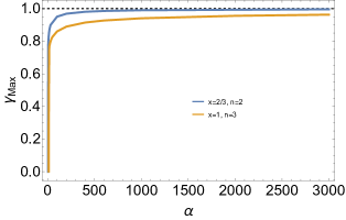
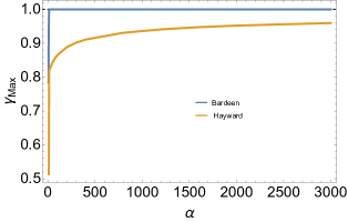
Figure 1: $\gamma_{max}$ as the function of $\alpha$, which is defined as $K^{max}(\gamma_{max})=1$ and obtained by scanning the mass of black holes. The left plot is for the regular black holes with asymptotically Minkowski core while the right plot is for the regular black holes with asymptotically de-Sitter core.

We argue that our above treatment is a dramatic improvement in comparison with the scheme applied in [26], where the maximal value of $\gamma$ is defined for a given mass. Because in next sections will find that for a given $\alpha$ and $\gamma$, Kretschmann curvature is sub-Planckian with some large mass does not guarantee that it must be sub-Planckian with any mass, even if it becomes saturated in large mass limit (this is always true indeed). On the contrary, Kretschmann curvature may exceed the Planck scale easily when the mass drops down. For instance, in Figure 6 of [26] which is on the modified Hayward black hole, $K$ is sub-Planckian for $M=10^{5}$, but if one drops down the mass with other parameters fixed, $K_{max}$ can easily exceed one. For instance, if $M=10^{2}$, then $K_{max}\simeq 6000$. In a word, the introduction of $\gamma_{max}$ independent of mass in our paper gives us a way to specify the parameter values such that the sub-Planckian feature of curvature can be preserved during the whole process of evaporation.

3 Modified regular black hole with $x=1$ and $n=2$

In this section we study the modified regular black hole with $n=2$ and $x=1$. When $G(r)=1$, its main features have been investigated in [1]. We remark that the following features are maintained when the metric is modified by $G(r)$. Firstly, the mass of the black hole is bounded by $M\geq\frac{e\alpha}{2}$. In particular, when this bound is saturated, the black hole is characterized by the minimal radius $r_{h}=\sqrt{e}\alpha_{0}$, which may be treated as the remnant of the black hole evaporation, since the final stage of the black hole is characterized by $M\rightarrow\frac{e\alpha_{0}}{2}$ (or $r_{h}\rightarrow\sqrt{e}\alpha_{0}$). This effect completely results from the exponential suppressing potential and is controlled by the parameter $\alpha$. In this limit, it is obvious to see that the Hawking temperature is always vanishing even when 1-loop quantum correction and time delay are incorporated, as illustrated in Fig.2. It is noticed that the maximal value of the temperature goes down with the increase of $\gamma$. In addition, based on the equations in Appendix.C we may plot the heat capacity as well as the entropy as the function of black hole mass. Whenever the temperature reaches the maximal value, the heat capacity becomes divergent, as illustrated in Fig.3, which means the black hole undergoes a transition from a system with negative heat capacity to a system with positive heat capacity during the process of evaporation. Since the black hole has a remnant with the minimal mass, whose entropy may be denoted as $S_{min}$, we may also plot the entropy difference between the black hole with any mass and the one with the minimal mass, as illustrated in Fig.3. It is found that the entropy difference monotonically decreases with the decrease of the mass $M$, but does not change much with the change of parameter $\gamma$. The inset of Fig.3 tells us that the entropy increases a little bit when $\gamma$ goes up with a given mass.

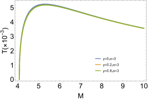
Figure 2: Left: The temperature as the function of $M$.   Right: The maximum value of temperature as the function of $\gamma$.

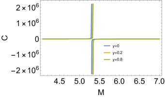
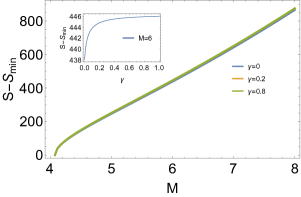
Figure 3: Left: The heat capacity as the function of $M$.   Right: The entropy as the function of $M$, while the inset shows the entropy as the function of $\gamma$ with a given mass.

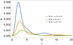
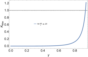
Figure 4: Left: The Kretschmann scalar curvature $K$ as the function of the radial coordinate $r$ with $\gamma=0.5$. Right:The maximum value of the Kretschmann scalar curvature $K$ as the function of $\gamma$.

Secondly, these exists a minimal value for $\alpha$ at the Planck scale $\alpha_{min}\simeq 2.747$ such that $K^{max}(\alpha_{min})=1$. When 1-loop quantum correction and time delay are incorporated, we find $\alpha_{min}$ does not change. For $\alpha\geq\alpha_{min}$, we may plot Kretschmann curvature $K$ as the function of the radial coordinate $r$, as shown in Fig.4. In general, the maximal value of $K$ appears at some position in space, and we denote it as $K_{max}$. Similar to the case with $G(r)=1$, we find $K(0)=0$ always, but the location of $K_{max}$ moves to the right side with the increase of mass $M$. We demonstrate $K_{max}$ as the function of $\gamma$ in the right plot of Fig.4, indicating that it monotonously grows up with the parameter $\gamma$ once $\alpha$ is fixed. Therefore, we need define a $\gamma_{max}$ to preserve Kretschmann curvature to be sub-Planckian.

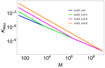
Figure 5: The maximum value of the Kretschmann scalar curvature $K$ as the function of $M$.

Finally, we illustrate the mass dependent behavior of $K_{max}$ in Fig.5. For $G(r)=1$, we have figured out in [1] that $K_{max}\propto 1/M$ such that the black hole with the minimal mass is featured by the maximal $K_{max}$. When $G(r)$ is turned on, we find in this figure that $K_{max}$ remains a linear relation with the logarithm of mass, thus decaying with the increase of mass. The main difference is that the value of $K_{max}$ is promoted due to the presence of $\gamma$.

4 Modified regular black hole with $x=2/3$ and $n=2$

In this section, we will study the modified regular black hole with $n=2$ and $x=2/3$, which corresponds to Bardeen black hole at large scales, since the gravitational potential of Bardeen black hole $\phi(r)$ is given as

$$\phi(r)=-\frac{Mr^{2}}{\left(\frac{2}{3}\alpha M^{2/3}+r^{2}\right)^{3/2}}.$$ (6)

One can easily check these two black holes have the same expansion behavior for large radius. Nevertheless, they have distinct behavior near the central core. The former has an asymptotically Minkowski core, while Bardeen black hole has a de-Sitter core.

Similarly, we point out that for the regular black hole with $x=2/3,\ n=2$, the mass is bounded by $M\geq\left(\frac{e}{2}\right)^{3/4}\alpha^{3/4}$, which is solely determined by the exponentially suppressing potential controlled by the parameter $\alpha$. Thus the presence of $G(r)$ does not change the whole picture of black hole evaporation, and the remnant of black holes maintains at the final stage. Again, $\alpha$ has the minimal value $\alpha_{min}\simeq 0.875$, that is defined by $K_{max}(\alpha_{min})=1$ with $\gamma=0$. While for Bardeen black hole, it is worthwhile to point out that $M\geq(\frac{9\alpha}{4})^{3}$, indicating that $M_{min}$ increases with $\alpha^{3}$. That is to say, $M_{min}$ grows rapidly with $\alpha>1$. This behavior is in contrast to all the other regular black holes in this paper.

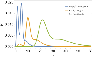
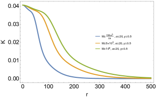
Figure 6: Kretschmann curvature $K$ as the function of the radial coordinate $r$ for $\gamma=0.5$. The left plot is for the regular black hole with $x=2/3,\ n=2$, while the right plot is for Bardeen black hole.

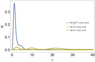
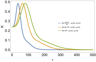
Figure 7: Kretschmann curvature $K$ as the function of the radial coordinate $r$ for $\gamma=0.8$. The left plot is for the regular black hole with $n=2,\ x=2/3$, while the right plot is for Bardeen black hole.

Now let us compare Kretschmann scalar curvature $K$ as the function of the radius $r$ for these two black holes. In Fig.6 we plot Kretschmann curvature $K(r)$ for $\gamma=0.5$, which is much smaller than $\gamma_{max}$. One finds $K(0)=0$ always for black hole with $x=2/3$ and $n=2$, while $K(0)=K_{max}$ for Bardeen black hole, irrespective of the mass of the black hole. While for $\gamma$ close to $\gamma_{max}$, for instance $\gamma=0.8$ as illustrated in Fig.7, the maximal value of $K$ runs away from the center for Bardeen black hole as well.

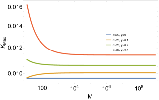
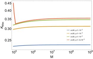
Figure 8: The maximum value of Kretschmann curvature $K_{max}$ as the function of $M$ for the black hole with $n=2,\ x=2/3$ (left) and Bardeen black hole (right).

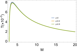
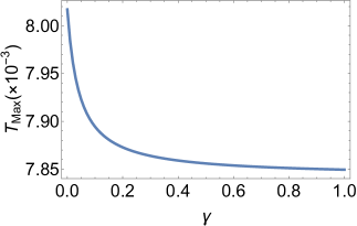
Figure 9: Left: The temperature as the functions of $M$.   Right: The maximum value of temperature as the functions of $\gamma$.

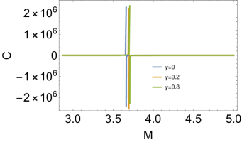
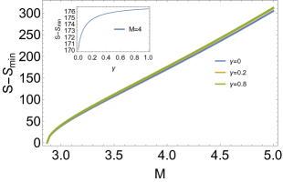
Figure 10: Left: The heat capacity as the function of $M$.   Right: The entropy as the function of $M$, while the inset shows the entropy as the function of $\gamma$ with a given mass.

Next we focus on the mass dependent behavior of $K_{max}$ for these two black holes. It is known in [1] that when $G(r)=1$, both black holes are characterized by the fact that $K_{max}$ is independent of the mass of black holes. However, when $G(r)$ is turned on we find this feature does not hold anymore. This is not surprising if one recalls that an arbitrarily large time delay would make the metric singular again. Therefore, in this case we demonstrate the mass dependent behavior of $K_{max}$ for different values of $\gamma$ in Fig.8. First of all, when $G(r)=1$, namely $\gamma=0$, $K_{max}$ is a constant indeed (see the left plot of Fig.8), while with the increase of $\gamma$, we notice that $K_{max}$ becomes larger and depends on the mass. In particular, it is surprising to notice that as $\gamma$ approaches $\gamma_{max}$, $K_{max}$ with small masses becomes larger, and this phenomenon is observed for both black hole with $x=2/3,\ n=2$ and Bardeen black hole, as illustrated in Fig.8 ($\gamma=0.4$ in the left plot while $\gamma=1-3\times 10^{-5}$ in the right plot). It is this fact that $K_{max}$ with small masses always grows up to one at first and determines the value of $\gamma_{max}$ when we scan the mass of black holes. This tendency also gives us more difficulty to figure out $\gamma_{max}$ by scanning the mass of black holes in Fig.1. On the other hand, $K_{max}$ always becomes saturated in large mass limit. This nice feature is important for us to pick out a $\gamma_{max}$ to preserve $K_{max}$ to be sub-Planckian always. In addition, we remark that for Bardeen black hole, the mass dependent behavior of $K_{max}$ does not change much until $\gamma\rightarrow\gamma_{max}$, and the mass scale is much larger than that for the black hole with $x=2/3,\ n=2$, which is the reflection of the fact $M_{min}\propto\alpha^{3}$ since we have set $\alpha=20$.

Finally, the thermodynamical behavior of the black hole is illustrated in Fig.9 and Fig.10. We find that the maximal value of the Hawking temperature becomes smaller slightly with the increase of $\gamma$, while the entropy becomes larger slightly with the increase of $\gamma$.

5 Modified regular black hole with $x=1$ and $n=3$

In this section we will study the modified regular black hole with $n=3$ and $x=1$ in a quite parallel manner, which corresponds to Hayward black hole at large scales. The gravitational potential for Hayward black hole is given by

$$\phi(r)=-\frac{Mr^{2}}{r^{3}+M\alpha}.$$ (7)

We plot Kretschmann curvature $K$ as the function of the radial coordinate $r$ in Fig.11, where $M=\frac{1}{2}\sqrt{\frac{3e\alpha}{2}}$ is the minimal value allowed for the regular black hole with $x=1$ and $n=3$, while $M=\frac{3}{4}\sqrt{\frac{3\alpha}{2}}$ is the minimal value allowed for Hayward black hole. It is found that $K_{max}$ moves to the right with larger radius as the mass increases for black hole with $x=1$ and $n=3$, while for Bardeen black hole $K_{max}$ runs away from the center as well.

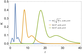
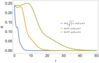
Figure 11: The Kretschmann scalar curvature $K$ as the functions of the radial coordinate $r$. The left plot is for the regular black hole with $n=3,\ x=1$, while the right plot is for Hayward black hole.

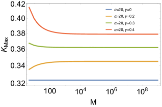
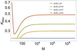
Figure 12: The maximum value of the Kretschmann scalar curvature $K$ as the function of $M$ for $n=3,\ x=1$(left) and Hayward black hole(right).

Next we focus on the mass dependent behavior of $K_{max}$. We plot $K_{max}$ as the function of $M$ for both black holes, as illustrated in Fig.12. The phenomenon is similar to what we have found in the previous section. This figure explicitly exhibits that $K_{max}$ does not depend on the mass of black holes when $\gamma=0$, as we expect. However, when the time delay parameter $\gamma$ is turned on, for instance $\gamma=0.2$ in the left plot and $\gamma=0.6,0.7$ in the right plot, we find $K_{max}$ increases with the mass and becomes saturated in the large mass limit. Keep increasing $\gamma$ further, one finds $K_{max}$ becomes larger on the side with small masses, for instance when $\gamma=0.3,0.4$ in the left plot and $\gamma=0.8$ in the right plot. In this situation, $K_{max}$ decreases with the mass and then becomes saturated in the large mass limit.

Finally, we remark that the thermodynamical behavior of this modified regular black hole is quite similar to what we have demonstrated in previous sections. The maximal value of the Hawking temperature becomes smaller slightly with the increase of $\gamma$, while the entropy becomes larger slightly with the increase of $\gamma$.

6 Conclusion and Discussion

In this paper we have developed the regular black holes recently proposed in [1] by incorporating the 1-loop quantum correction to the gravity potential and a time delay between an observer at the center and the one at infinity. Our analysis covers two sorts of black holes. One is featured by an asymptotically Minkowski core, while the other is featured by an asymptotically de-Sitter core. We have proposed a scheme to figure out the maximal time delay at the center by scanning the mass of black holes such that the sub-Planckian feature of Kretschmann curvature is preserved for black holes during the whole evaporation process, which greatly improved the strategy presented in [26] where the maximal time delay is considered for a given mass in the context of modified Hayward black hole. Therefore, such effective metrics may be more appropriate to be applied to describe the evolution of Planck stars or the evaporation of black holes. We have also compared the distinct behavior of Kretschmann curvature for these two sorts of black holes. In general, we have found the mass dependent behavior of $K_{max}$ becomes complicated when 1-loop quantum correction and the time delay are taken into account. Nevertheless, it is still plausible to define a modified regular black hole with sub-Planckian curvature irrespective of the mass, thanks to the saturating behavior of $K_{max}$ in the large mass limit.

Next we remark that the form of $G(r)$ adopted in this paper is not unique of course. One may consider other forms of $G(r)$, for instance $G(r)=1-\gamma+\gamma e^{\frac{-\beta M}{\gamma r^{3}}}$ as proposed in [27], to introduce 1-loop quantum correction and the time delay. One would obtain the similar results. More importantly, we may further improve the form of effective metric to be more practical to describe the collapse of star or black holes. One prominent issue in all previous papers is that one just introduces the time delay by hand, since $\gamma$ is introduced as a free parameter. A more realistic setup would be that the time delay is fixed to be a specific one by the distribution of matter surrounding the center. At the phenomenological level, it implies that $\gamma$ could be determined by the other parameters or quantities. For instance, we could assume that $\gamma=1-(\alpha_{min}/\alpha)^{1/n}$ or $\gamma=1-(\alpha_{min}/\alpha)^{1/(n-1)}$, then remarkably we find this value is always smaller than $\gamma_{max}$ for arbitrary value of $\alpha$ such that a sub-Planckian Kretschmann scalar curvature is always guaranteed. We expect this conjecture can be justified by more detailed investigation in future.

Finally, at the current stage we are strict to consider the regular black holes with spherical symmetry. We expect the proposed construction may be extended to the rotating black holes, as other authors have performed for Hayward black holes in [18, 27].

Appendix A The Kretschmann scalar curvature

For ansatz in Eq.(1), it is straightforward to derive the Kretschmann scalar curvature which is given by

$$K =R^{\mu\nu\rho\lambda}R_{\mu\nu\rho\lambda}$$ (8)

$$=\frac{(2\phi(r)+1)^{2}G^{\prime}(r)^{4}}{4G(r)^{4}}+4\left(\frac{4\left(r^{2}\phi^{\prime}(r)^{2}+\phi(r)^{2}\right)}{r^{4}}+\phi^{\prime\prime}(r)^{2}\right)$$

$$+\frac{1}{r^{2}G(r)^{2}}(r^{2}(2\phi(r)+1)^{2}G^{\prime\prime}(r)^{2}+G^{\prime}(r)^{2}(-2r^{2}(2\phi(r)+1)\phi^{\prime\prime}(r)$$

$$+9r^{2}\phi^{\prime}(r)^{2}+8\phi(r)^{2}+8\phi(r)+2)+6r^{2}(2\phi(r)+1)G^{\prime}(r)G^{\prime\prime}(r)\phi^{\prime}(r))$$

$$-\frac{1}{G(r)^{3}}((2\phi(r)+1)G^{\prime}(r)^{2}\left((2\phi(r)+1)G^{\prime\prime}(r)+3G^{\prime}(r)\phi^{\prime}(r)\right))$$

$$+\frac{1}{r^{2}G(r)}(4\left(r^{2}(2\phi(r)+1)G^{\prime\prime}(r)\phi^{\prime\prime}(r)+G^{\prime}(r)\phi^{\prime}(r)\left(3r^{2}\phi^{\prime\prime}(r)+4\phi(r)+2\right)\right)).$$

Furthermore, if we expect that $G(r)$ only plays a role of time delay at the center, without changing the asymptotical behavior near the center, it is reasonable to require that $G^{\prime}(0)=G^{\prime\prime}(0)=0$. Then, as $r\rightarrow 0$, we find Kretschmann scalar curvature behaves as

$$K\sim 4\phi^{\prime\prime}(r)^{2}+\frac{16\phi^{\prime}(r)^{2}}{r^{2}}+\frac{16\phi(r)^{2}}{r^{4}}.$$ (9)

Remarkably, we find the function $G(r)$ would not change the value of Kretschmann scalar curvature at the center, under the condition that $G^{\prime}(0)=G^{\prime\prime}(0)=0$.

Appendix B The horizon of the modified regular black hole

In this section, we derive the location of the outer horizon for the modified regular black hole, where the metric components are specified by Eq.(3). First of all, we notice that the location of the outer horizon is not affected by $G(r)$, it is solely determined by $F(r_{h})=0$ and this gives rise to the relation between $r_{h}$ and $M$:

$$2M=r_{h}e^{\alpha M^{x}/r_{h}^{n}}.$$ (10)

We rewrite the radius of the horizon $r_{h}$ as

$$r_{h}=2M\left(\frac{\theta}{W(\theta)}\right)^{1/n},\quad\theta=-\frac{\alpha}{2M^{2-x}},$$ (11)

where

$$W(\theta)=\sum_{n=1}^{\infty}\frac{(-n)^{n-1}}{n!}\theta^{n},$$ (12)

is the Lambert-W function with $W(\theta)\geq-1$. A real W requires $\theta\geq-e^{-1}$, thus the mass of modified regular black hole is bounded by

$$M\geq\frac{1}{2}(e\alpha)^{\frac{1}{2-x}}.$$ (13)

Appendix C The thermodynamics of the modified black holes

For the modified black holes with non-trivial $G(r)$, the black hole temperature and the luminosity are respectively given by

$$T =\left[-\frac{1}{4\pi}\sqrt{-g^{tt}g^{rr}}\frac{d}{dr}g_{tt}\right]_{r=r_{h}}=\frac{\left(2\phi\left(r_{h}\right)+1\right)G^{\prime}\left(r_{h}\right)+2G\left(r_{h}\right)\phi^{\prime}\left(r_{h}\right)}{4\pi\sqrt{G\left(r_{h}\right)}},$$ (14)

$$L =\sigma T^{4}A=\frac{\sigma r_{h}^{2}\left(\left(2\phi\left(r_{h}\right)+1\right)G^{\prime}\left(r_{h}\right)+2G\left(r_{h}\right)\phi^{\prime}\left(r_{h}\right)\right){}^{4}}{64\pi^{3}G\left(r_{h}\right){}^{2}}.$$

Using Eq.(11) and (14), one can derive the heat capacity as

$$C=\frac{dM}{dT}=\frac{dM/dr_{h}}{dT/dr_{h}}.$$ (15)

Moreover, according to the first law of black hole thermodynamics, the entropy of the modified black hole is given by

$$S=\int\frac{dM}{T}.$$ (16)

Usually, due to the correction of the Hawking temperature, it is well known that the entropy of modified black holes will deviate from the area law and receive the higher order corrections. For instance, for Hayward black hole in [28], the integrated form of the entropy can be expanded as

$$S=\pi r_{h}^{2}+\pi\alpha\log\left(2r_{h}^{2}-\alpha\right)-\frac{\pi\alpha}{2}-\frac{\pi\alpha^{2}}{2\left(2r_{h}^{2}-\alpha\right)}.$$ (17)

For Bardeen black hole in [29], the integrated form of the entropy is given by

$$S=2\pi\left(\left(\frac{r_{h}}{2}-\frac{\alpha}{r_{h}}\right)\sqrt{\alpha+r_{h}^{2}}+\frac{3}{2}\alpha\log\left(\sqrt{\alpha+r_{h}^{2}}+r_{h}\right)\right).$$ (18)

For regular black hole in [19], the integrated form of the entropy can be written as

$$S=\int\frac{dM}{T}=e^{\frac{\alpha}{r_{h}^{2}}}\pi r_{h}^{2}+2\pi\alpha\int\frac{e^{\frac{\alpha}{r_{h}^{2}}}}{r_{h}}\,dr_{h}.$$ (19)

For the black hole presented in this paper, such expansions become very complicated and we just present the numerical results in the main body of the text.

References

- [1] Y. Ling and M. H. Wu, [arXiv:2109.05974 [gr-qc]].
- [2] R. J. Adler, P. Chen and D. I. Santiago, Gen. Rel. Grav. 33, 2101-2108 (2001) [arXiv:gr-qc/0106080 [gr-qc]].
- [3] G. Amelino-Camelia, M. Arzano and A. Procaccini, Phys. Rev. D 70, 107501 (2004) doi:10.1103/PhysRevD.70.107501 [arXiv:gr-qc/0405084 [gr-qc]].
- [4] A. Ashtekar and M. Bojowald, Class. Quant. Grav. 22, 3349-3362 (2005) [arXiv:gr-qc/0504029 [gr-qc]].
- [5] G. Amelino-Camelia, M. Arzano, Y. Ling and G. Mandanici, Class. Quant. Grav. 23, 2585-2606 (2006) [arXiv:gr-qc/0506110 [gr-qc]].
- [6] Y. Ling, B. Hu and X. Li, Phys. Rev. D 73, 087702 (2006) [arXiv:gr-qc/0512083 [gr-qc]].
- [7] Y. Ling, X. Li and H. b. Zhang, Mod. Phys. Lett. A 22, 2749-2756 (2007) [arXiv:gr-qc/0512084 [gr-qc]].
- [8] A. Bonanno and M. Reuter, Phys. Rev. D 62, 043008 (2000) [arXiv:hep-th/0002196 [hep-th]].
- [9] C. Rovelli and F. Vidotto, Int. J. Mod. Phys. D 23, no.12, 1442026 (2014) [arXiv:1401.6562 [gr-qc]].
- [10] J. M. Bardeen, In Proceeding of the international conference GR5, 1968, Tbilisi, USSR, Georgia, pp. 174-180.
- [11] S. A. Hayward, Phys. Rev. Lett. 96, 031103 (2006) [arXiv:gr-qc/0506126 [gr-qc]].
- [12] V. P. Frolov, JHEP 05, 049 (2014) [arXiv:1402.5446 [hep-th]].
- [13] A. Bogojevic and D. Stojkovic, Phys. Rev. D 61, 084011 (2000) [arXiv:gr-qc/9804070 [gr-qc]].
- [14] P. O. Mazur and E. Mottola, [arXiv:gr-qc/0109035 [gr-qc]].
- [15] I. Dymnikova, Class. Quant. Grav. 19, 725-740 (2002) [arXiv:gr-qc/0112052 [gr-qc]].
- [16] P. Nicolini, A. Smailagic and E. Spallucci, Phys. Lett. B 632, 547-551 (2006) [arXiv:gr-qc/0510112 [gr-qc]].
- [17] K. Falls, D. F. Litim and A. Raghuraman, Int. J. Mod. Phys. A 27, 1250019 (2012) [arXiv:1002.0260 [hep-th]].
- [18] C. Bambi and L. Modesto, Phys. Lett. B 721, 329-334 (2013) [arXiv:1302.6075 [gr-qc]].
- [19] L. Xiang, Y. Ling and Y. G. Shen, Int. J. Mod. Phys. D 22, 1342016 (2013) [arXiv:1305.3851 [gr-qc]].
- [20] H. Culetu, [arXiv:1305.5964 [gr-qc]].
- [21] H. Culetu, Int. J. Theor. Phys. 54, no.8, 2855-2863 (2015) [arXiv:1408.3334 [gr-qc]].
- [22] S. G. Ghosh, Eur. Phys. J. C 75, no.11, 532 (2015) [arXiv:1408.5668 [gr-qc]].
- [23] A. Simpson and M. Visser, Universe 6, no.1, 8 (2019) [arXiv:1911.01020 [gr-qc]].
- [24] N. E. J. Bjerrum-Bohr, J. F. Donoghue and B. R. Holstein, Phys. Rev. D 67, 084033 (2003) [erratum: Phys. Rev. D 71, 069903 (2005)] [arXiv:hep-th/0211072 [hep-th]].
- [25] J. F. Donoghue, AIP Conf. Proc. 1483, no.1, 73-94 (2012) [arXiv:1209.3511 [gr-qc]].
- [26] T. De Lorenzo, C. Pacilio, C. Rovelli and S. Speziale, Gen. Rel. Grav. 47, no.4, 41 (2015) [arXiv:1412.6015 [gr-qc]].
- [27] T. De Lorenzo, A. Giusti and S. Speziale, Gen. Rel. Grav. 48, no.3, 31 (2016) [erratum: Gen. Rel. Grav. 48, no.8, 111 (2016)] [arXiv:1510.08828 [gr-qc]].
- [28] X. Li, Y. Ling, Y. G. Shen, C. Z. Liu, H. S. He and L. F. Xu, Annals Phys. 396, 334-350 (2018) [arXiv:1611.09016 [gr-qc]].
- [29] M. Sharif and W. Javed, J. Korean Phys. Soc. 57, 217-222 (2010) [arXiv:1007.4995 [gr-qc]].