Preconditioning for finite element methods with strain smoothing

Abstract

Strain smoothing methods such as the smoothed finite element methods (S-FEMs) and the strain-smoothed element method (SSE) have successfully improved the convergence behavior of finite elements. The strain smoothing methods have been applied in numerous finite element analyses, especially for analyzing solids and structures; however, there have been no studies on efficient numerical solvers for the methods. We need mathematically and numerically well-elaborated iterative solvers for efficient applications to large-scale problems. In this study, we investigate how to design appropriate preconditioners for the methods with inspiration from the spectral properties of the strain smoothing methods. First, we analyze the spectrums of the stiffness matrices of the edge-based S-FEM and SSE. Subsequently, we propose improved two-level additive Schwarz preconditioners for the strain smoothing methods by modifying local solvers appropriately. For convenience of implementation, an alternative form of the preconditioners is proposed by defining the coarse-scale operation in terms of the standard FEM. We verify our theoretical results through numerical experiments.

url]https://sites.google.com/view/jonghopark

1 Introduction

There have been various attempts to improve the performance of finite elements, among which strain smoothing methods can achieve the goal without introducing additional degrees of freedom. Chen et al. [1] first proposed the concept of strain smoothing methods for the Galerkin mesh-free method. Subsequently, Liu et al. [2] applied the strain smoothing technique to the finite element method (FEM) and developed a series of smoothed FEMs (S-FEMs). The S-FEMs are classified according to the construction of smoothing domains; the edge-based S-FEM (ES-FEM) and node-based S-FEM (NS-FEM) are well-known and broadly used [3, 4, 5, 6, 7]. The ES-FEM generally exhibits the best convergence properties among the S-FEMs [4]; the NS-FEM is effective in relieving volumetric locking [3]. Several studies were conducted to establish the theoretical properties of the S-FEMs [5, 8, 9]. Recently, the strain-smoothed element method (SSE) has been developed [10, 11, 12, 13, 14]. Whereas the S-FEMs construct strain fields for specifically defined smoothing domains, the SSE constructs strain fields for elements. The SSE provides a finite element solution with reduced discretization error by fully using the strains of all neighboring elements for strain smoothing. A theoretical foundation for the convergence properties of the SSE has been established in [15].

Although there has been a vast literature on the development of new strain smoothing methods and their applications to various engineering problems (see [16] for a recent survey), there have been no studies on efficient numerical solvers for the strain smoothing methods, to the best of our knowledge. However, developing robust and efficient numerical solvers is critical for successful application of the methods to large-scale engineering problems [17]. Particularly, iterative solvers are suitable for large-scale sparse linear problems [18]. Since the performance of iterative solvers relies on the condition number of a target linear system, an effective way to improve iterative solvers is to design good preconditioners. In this perspective, there have been plenty of notable works on preconditioning of large-scale linear problems arising in structural mechanics; see, e.g., [19, 20, 21, 22].

In this study, we examine how to design suitable preconditioners for the strain smoothing methods. The main observation is that the stiffness matrices of the ES-FEM and SSE are spectrally equivalent to that of the standard FEM. This observation guarantees that the ES-FEM and SSE can adopt any preconditioner designed for the standard FEM and enjoy the advantages of the preconditioner such as good conditioning or numerical scalability. As a concrete example, we consider an overlapping Schwarz preconditioner, which is one of the most broadly used parallel preconditioners for finite element problems [23, 24, 25, 26]. We prove that the standard two-level additive Schwarz preconditioner [23] designed for the standard FEM can be applied to the ES-FEM and SSE, satisfying the condition number bound $C(1+H/\delta)$, where $C$ is a positive constant independent of the mesh and subdomain sizes, $H$ is the subdomain size, and $\delta$ is the overlapping width for the overlapping domain decomposition associated with the additive Schwarz preconditioner. Additionally, we propose novel improved two-level additive Schwarz preconditioners for the ES-FEM and SSE with better condition number estimates than the standard two-level additive Schwarz preconditioner. With some simple modifications on the local problems of the standard Schwarz preconditioner, we obtain the proposed preconditioners that show improved performance in both theoretical and numerical senses. The improvement strategy can be applied to not only additive Schwarz preconditioners but also a broad range of subspace correction preconditioners [27, 28] such as multigrid and domain decomposition preconditioners. Notably, several existing iterative solvers for linear systems fit into the framework of subspace correction [27]; the improvement strategy introduced in this study reveals new possibilities for designing efficient iterative solvers for various contemporary FEMs. Numerical results verify the theories presented in this study and prove the superiority of the proposed improved preconditioners.

This study includes an interesting remark on the NS-FEM; although the NS-FEM and ES-FEM are considered members of the common class of S-FEMs, their spectral properties may differ significantly. In this study, we claim that the stiffness matrix of the NS-FEM may not be spectrally equivalent to that of the standard FEM. Specifically, we present an example that the condition number $\kappa(K^{-1}\bar{K}_{\mathrm{NS}})$ increases as the mesh size $h$ decreases, where $K$ and $\bar{K}_{\mathrm{NS}}$ are the stiffness matrices of the standard FEM and NS-FEM, respectively. This suggests the need to develop different mathematical theories for the NS-FEM and ES-FEM. However, most of the existing theories [5, 9, 16] are based on a unified S-FEM framework.

The remainder of this paper is organized as follows. In Section 2, we summarize the key features of the ES-FEM and SSE. Section 3 deals with the spectral properties of the ES-FEM and SSE; specifically, we demonstrate that the stiffness matrices of these methods are spectrally equivalent to that of the standard FEM. Utilizing the spectral equivalence, in Section 4, we present efficient two-level additive Schwarz preconditioners for the ES-FEM and SSE and analyze their convergence properties. Section 5 presents numerical results that support the theoretical findings. In Section 6, we give some remarks on the spectral property of the NS-FEM. We conclude the study in Section 7.

2 Finite element methods with strain smoothing

We provide brief descriptions of the S-FEM and SSE for a model Poisson problem

$$\begin{split}-\Delta u=f\quad&\textrm{ in }\Omega,\\ u=0\quad&\textrm{ on }\partial\Omega,\end{split}$$ (2.1)

where $\Omega\subset\mathbb{R}^{2}$ is a bounded polygonal domain. For simplicity, we consider the case of three-node triangular elements throughout this study; see [29] and [12] for formulations of polygonal finite elements adopting the S-FEM and SSE, respectively. For a subregion $\omega\subset\Omega$ and a nonnegative integer $n$, the collection of all polynomials of degree less than or equal to $n$ on $\omega$ is denoted by $\mathcal{P}_{n}(\omega)$. Let $\mathcal{T}_{h}$ be a quasi-uniform triangulation of $\Omega$ with a characteristic element diameter $h>0$. We define $V_{h}$ as the conforming piecewise linear finite element space on $\mathcal{T}_{h}$, i.e.,

$$V_{h}=\left\{v\in H_{0}^{1}(\Omega):v|_{e}\in\mathcal{P}_{1}(e)\hskip 2.84544pt\forall e\in\mathcal{T}_{h}\right\},$$

where $H_{0}^{1}(\Omega)$ is the usual Sobolev space consisting of all functions $u\in L^{2}(\Omega)$ such that $\nabla u\in(L^{2}(\Omega))^{2}$ and $u|_{\partial\Omega}=0$. We also define $W_{h}$ as follows:

$$W_{h}=\left\{\epsilon\in(L^{2}(\Omega))^{2}:\epsilon|_{e}\in(\mathcal{P}_{0}(e))^{2}\hskip 2.84544pt\forall e\in\mathcal{T}_{h}\right\}.$$

Then we readily have that $v\in V_{h}$ implies $\nabla v\in W_{h}$. With a slight abuse of notation, we do not distinguish between finite element functions and the corresponding vectors of degrees of freedom in the following.

2.1 Standard finite element method

The geometry of a 3-node triangular element $e\in\mathcal{T}_{h}$ is interpolated by

$$(x,y)=\sum_{i=1}^{3}h_{i}(r,s)(x_{i},y_{i})\in e,$$

where $(x_{i},y_{i})$, $1\leq i\leq 3$, is the position vector of the $i$th node of $e$ in the global Cartesian coordinate system, and $h_{i}(r,s)$ is the two-dimensional interpolation function of the standard isoparametric procedure corresponding to the $i$th node, that is, $h_{1}(r,s)=1-r-s$, $h_{2}(r,s)=r$, and $h_{3}(r,s)=s$. The corresponding interpolation of the function $u$ within the element $e$ is given by

$$u(x,y)=\sum_{i=1}^{3}h_{i}(r,s)u_{i},$$

where $u_{i}=u(x_{i},y_{i})$. Note that $u$ is continuous and piecewise linear on $\mathcal{T}_{h}$, i.e., $u\in V_{h}$.

The local gradient $\epsilon^{(e)}$ within element $e$ is obtained through the standard isoparametric finite element procedure as follows:

$$\epsilon^{(e)}=B^{(e)}u^{(e)}\quad\textrm{with}\quad B^{(e)}=\begin{bmatrix}\frac{\partial h_{1}}{\partial x}&\frac{\partial h_{2}}{\partial x}&\frac{\partial h_{3}}{\partial x}\\ \frac{\partial h_{1}}{\partial y}&\frac{\partial h_{2}}{\partial y}&\frac{\partial h_{3}}{\partial y}\end{bmatrix},\hskip 2.84544ptu^{(e)}=\begin{bmatrix}u_{1}&u_{2}&u_{3}\end{bmatrix}^{T}.$$ (2.2)

The stiffness matrix $K$ corresponding to the standard FEM is given by

$$u^{T}Kv=\int_{\Omega}\nabla u\cdot\nabla v\,d\Omega=\sum_{e\in\mathcal{T}_{h}}|e|\left(B^{(e)}u^{(e)}\right)^{T}\left(B^{(e)}v^{(e)}\right),\quad u,v\in V_{h}.$$ (2.3)

A finite element solution corresponding to the standard FEM is given by a solution of a linear system

$$Ku=f,$$

where the load vector $f$ is defined as

$$f^{T}v=\int_{\Omega}fv\,d\Omega,\quad v\in V_{h}.$$ (2.4)

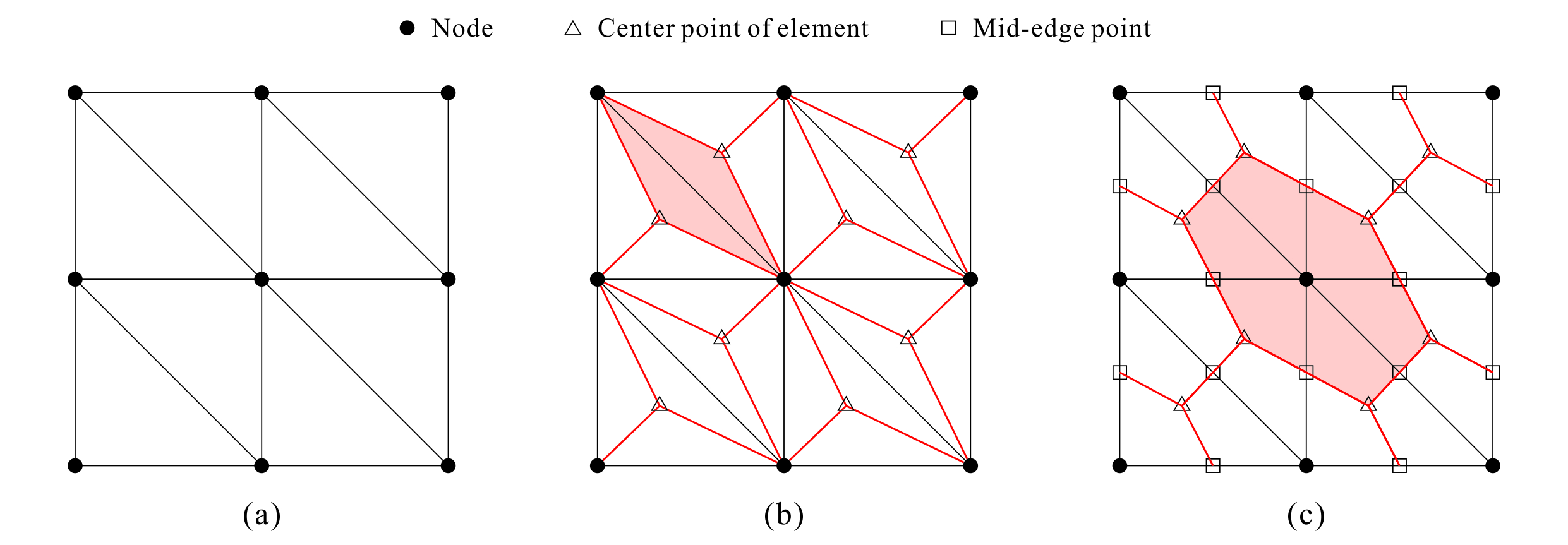
Figure 1: Discretizations based on (a) finite elements, (b) edge-based smoothing domains, and (c) node-based smoothing domains.

2.2 Edge-based smoothed finite element method (ES-FEM)

The standard FEM discretizes a region into finite elements (see Fig. 1(a)), whereas S-FEM performs discretization based on newly defined smoothing domains. The well-known S-FEMs are the ES-FEM and NS-FEM, which form the smoothing domains based on the edges and nodes of $\mathcal{T}_{h}$, respectively. We briefly introduce the ES-FEM; see Section 6 for a description of the NS-FEM.

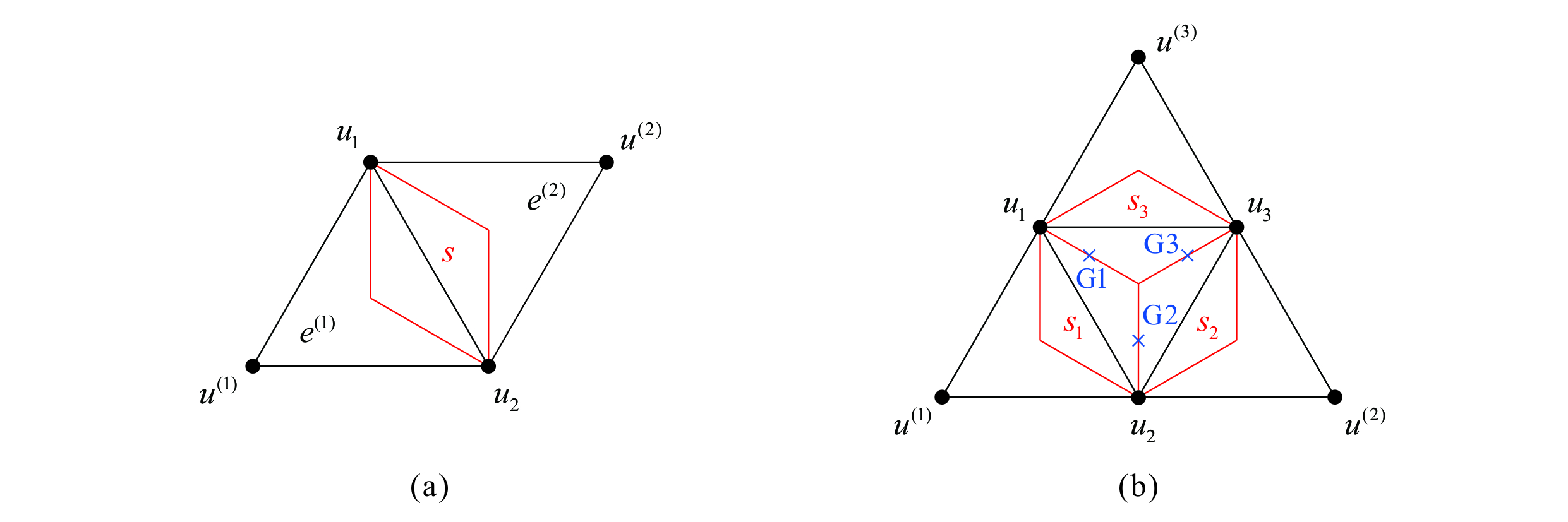
Figure 2: Degrees of freedom of $u\in V_{h}$ corresponding to the vectors (a) $\bar{u}^{(s)}$ in (2.6) and (b) $\bar{u}^{(e)}$ in (2.10).

In the ES-FEM, each element in $\mathcal{T}_{h}$ is divided into three triangular subdomains using its nodes and the barycenter ($r=s=1/3$). Subsequently, the edge-based smoothing domains are defined as assemblages of two neighboring subdomains belonging to different elements; see Fig. 1(b). In the following, let $\mathcal{S}_{h,\mathrm{ES}}$ denote the collection of all smoothing domains constructed from $\mathcal{T}_{h}$ for the ES-FEM. We define $W_{h,\mathrm{ES}}$ as the collection of all piecewise constant vector fields on $\mathcal{S}_{h,\mathrm{ES}}$, i.e.,

$$W_{h,\mathrm{ES}}=\left\{\epsilon\in(L^{2}(\Omega))^{2}:\epsilon|_{e}\in(\mathcal{P}_{0}(e))^{2}\hskip 2.84544pt\forall e\in\mathcal{S}_{h,\mathrm{ES}}\right\}.$$

The ES-FEM smoothing operator $S_{h,\mathrm{ES}}\colon W_{h}\rightarrow W_{h,\mathrm{ES}}$ that maps a given gradient field $\epsilon\in W_{h}$ to the corresponding smoothed gradient field $\bar{\epsilon}\in W_{h,\mathrm{ES}}$ is defined as follows. The local smoothed gradient $\bar{\epsilon}^{(s)}$ for a smoothing domain $s\in\mathcal{S}_{h,\mathrm{ES}}$ is defined by

$$\bar{\epsilon}^{(s)}=\frac{|e^{(1)}|\epsilon^{(e^{(1)})}+|e^{(2)}|\epsilon^{(e^{(2)})}}{|e^{(1)}|+|e^{(2)}|},$$ (2.5)

where $e^{(1)}$ and $e^{(2)}$ are the elements in $\mathcal{T}_{h}$ sharing the edge corresponding to $s$, and $\epsilon^{(e^{(1)})}$ and $\epsilon^{(e^{(2)})}$ were defined in (2.2). The local smoothed gradient in (2.5) can be expressed in a matrix-vector form as

$$\bar{\epsilon}^{(s)}=\bar{B}_{\mathrm{ES}}^{(s)}\bar{u}^{(s)}\quad\textrm{with}\quad\bar{B}_{\mathrm{ES}}^{(s)}=\frac{|e^{(1)}|}{|e^{(1)}|+|e^{(2)}|}B^{(e_{1})}R^{(e_{1})}+\frac{|e^{(2)}|}{|e^{(1)}|+|e^{(2)}|}B^{(e_{2})}R^{(e_{2})},\hskip 2.84544pt\bar{u}^{(s)}=\begin{bmatrix}u_{1}&u_{2}&u^{(1)}&u^{(2)}\end{bmatrix}^{T},$$ (2.6)

where the vector $\bar{u}^{(s)}$ consists of the four degrees of freedom of $u\in V_{h}$ at the nodes of the elements sharing the edge corresponding to $s$ as shown in Fig. 2(a), $B^{(e_{1})}$ and $B^{(e_{2})}$ were defined in (2.2), and $R^{(e_{1})}$ and $R^{(e_{2})}$ are boolean matrices that extract the degrees of freedom corresponding to the elements $e_{1}$ and $e_{2}$, respectively, i.e.,

$$R^{(e_{1})}=\begin{bmatrix}1&0&0&0\\ 0&1&0&0\\ 0&0&1&0\end{bmatrix},\hskip 2.84544ptR^{(e_{2})}=\begin{bmatrix}1&0&0&0\\ 0&1&0&0\\ 0&0&0&1\end{bmatrix}.$$

Finally, the stiffness matrix $\bar{K}_{\mathrm{ES}}$ for the ES-FEM can be obtained as

$$u^{T}\bar{K}_{\mathrm{ES}}v=\int_{\Omega}\bar{\nabla}_{\mathrm{ES}}u\cdot\bar{\nabla}_{\mathrm{ES}}v\,d\Omega=\sum_{s\in\mathcal{S}_{h,\mathrm{ES}}}|s|\left(\bar{B}_{\mathrm{ES}}^{(s)}\bar{u}^{(s)}\right)^{T}\left(\bar{B}_{\mathrm{ES}}^{(s)}\bar{v}^{(s)}\right),\quad u,v\in V_{h},$$ (2.7)

where $\bar{\nabla}_{\mathrm{ES}}$ denotes the global smoothed gradient operator corresponding to (2.5), i.e., $\bar{\nabla}_{\mathrm{ES}}=S_{h,\mathrm{ES}}\nabla$. We obtain an ES-FEM finite element solution by solving a linear system

$$\bar{K}_{\mathrm{ES}}u=f,$$

where the load vector $f$ was given in (2.4). That is, the ES-FEM uses an alternative stiffness matrix $\bar{K}_{\mathrm{ES}}$, whereas its load vector $f$ is the same as that of the standard FEM. Among the various types of S-FEMs, it has been numerically verified that the ES-FEM is the most effective method in reducing the discretization error of the finite element solution; see, e.g., [4].

2.3 Strain-smoothed element method (SSE)

When the SSE is employed, a smoothed gradient field is constructed for each element in $\mathcal{T}_{h}$ and the gradient information in all elements adjacent to a target element is utilized. No smoothing domains are required; the domain discretization with the SSE is the same as the one with the standard FEM. The space $W_{h,\mathrm{SSE}}$ for the SSE smoothed gradient fields is given by

$$W_{h,\mathrm{SSE}}=\left\{\epsilon\in(L^{2}(\Omega))^{2}:\epsilon|_{e}\in(\mathcal{P}_{1}(e))^{2}\hskip 2.84544pt\forall e\in\mathcal{T}_{h}\right\}.$$

Note that $W_{h,\mathrm{SSE}}$ includes piecewise linear polynomials, while $W_{h}$ only includes piecewise constant functions. We present how to construct the SSE smoothed gradient $\bar{\epsilon}=S_{h,\mathrm{SSE}}\epsilon\in W_{h,\mathrm{SSE}}$ for $\epsilon\in W_{h}$, where $S_{h,\mathrm{SSE}}\colon W_{h}\rightarrow W_{h,\mathrm{SSE}}$ denotes the SSE smoothing operator. For an element $e\in\mathcal{T}_{h}$, there can be up to three neighboring elements in $\mathcal{T}_{h}$ through element edges, say $e^{(k)}$, $1\leq k\leq 3$. An intermediate smoothed gradient $\hat{\epsilon}^{(k)}$ between $e$ and its neighboring element $e^{(k)}$ is defined by

$$\hat{\epsilon}^{(k)}=\frac{|e|\epsilon^{(e)}+|e^{(k)}|\epsilon^{(e^{(k)})}}{|e|+|e^{(k)}|},$$ (2.8)

where $\epsilon^{(e)}$ and $\epsilon^{(e^{(k)})}$ were defined in (2.2). If there is no adjacent element $e^{(k)}$ for some $k$, we simply use $\hat{\epsilon}^{(k)}=\epsilon^{(e)}$. Subsequently, we construct a linear smoothed gradient field $\bar{\epsilon}^{(e)}$ on the target element $e$ by unifying the intermediate smoothed gradients in (2.8). The values are assigned at three Gaussian integration points $\mathrm{G}k$, $1\leq k\leq 3$, of $e$ as the pointwise values of $\bar{\epsilon}^{(e)}$ as follows:

$$\bar{\epsilon}^{(e)}(\mathrm{G}k)=\frac{\hat{\epsilon}^{(k-1)}+\hat{\epsilon}^{(k)}}{2},$$ (2.9)

with the convention $\hat{\epsilon}^{(0)}=\hat{\epsilon}^{(3)}$. The smoothed gradient field $\bar{\epsilon}^{(e)}$ is uniquely determined within $e$ by linear interpolation of the pointwise values. The local smoothed gradient in (2.9) can be expressed in a matrix-vector form as

$$\bar{\epsilon}^{(e)}=\bar{B}_{\mathrm{SSE}}^{(e)}\bar{u}^{(e)}\quad\textrm{with}\quad\bar{B}_{\mathrm{SSE}}^{(e)}=\frac{1}{2}\begin{bmatrix}\bar{B}_{\mathrm{ES}}^{(s_{1})}R^{(s_{1})}+\bar{B}_{\mathrm{ES}}^{(s_{3})}R^{(s_{3})}\\ \bar{B}_{\mathrm{ES}}^{(s_{1})}R^{(s_{1})}+\bar{B}_{\mathrm{ES}}^{(s_{2})}R^{(s_{2})}\\ \bar{B}_{\mathrm{ES}}^{(s_{2})}R^{(s_{2})}+\bar{B}_{\mathrm{ES}}^{(s_{3})}R^{(s_{3})}\end{bmatrix},\hskip 2.84544pt\bar{u}^{(e)}=\begin{bmatrix}u_{1}&u_{2}&u_{3}&u^{(1)}&u^{(2)}&u^{(3)}\end{bmatrix}^{T},$$ (2.10)

where the vector $\bar{\epsilon}^{(e)}$ comprises three pointwise values $\bar{\epsilon}^{(e)}(\mathrm{G}1)$, $\bar{\epsilon}^{(e)}(\mathrm{G}2)$, and $\bar{\epsilon}^{(e)}(\mathrm{G}3)$, the vector $\bar{u}^{(e)}$ consists of at most six degrees of freedom of $u\in V_{h}$ at the nodes of $e$ and its neighboring elements (see Fig. 2(b)), the matrices $\bar{B}_{\mathrm{ES}}^{(s_{k})}$, $1\leq k\leq 3$, were defined in (2.6), and $R^{(s_{k})}$ are boolean matrices that extract the degrees of freedom corresponding to the subdomains $s_{k}$, i.e.,

$$R^{(s_{1})}=\begin{bmatrix}1&0&0&0&0&0\\ 0&1&0&0&0&0\\ 0&0&0&1&0&0\\ 0&0&1&0&0&0\end{bmatrix},\hskip 2.84544ptR^{(s_{2})}=\begin{bmatrix}0&1&0&0&0&0\\ 0&0&1&0&0&0\\ 0&0&0&0&1&0\\ 1&0&0&0&0&0\end{bmatrix},\hskip 2.84544ptR^{(s_{3})}=\begin{bmatrix}0&0&1&0&0&0\\ 1&0&0&0&0&0\\ 0&0&0&0&0&1\\ 0&1&0&0&0&0\end{bmatrix}.$$

In the SSE, the smoothed gradient field is constructed for each element in $\mathcal{T}_{h}$. The stiffness matrix $\bar{K}_{\mathrm{SSE}}$ for the SSE is calculated by

$$u^{T}\bar{K}_{\mathrm{SSE}}v=\int_{\Omega}\bar{\nabla}_{\mathrm{SSE}}u\cdot\bar{\nabla}_{\mathrm{SSE}}v\,d\Omega=\sum_{e\in\mathcal{T}_{h}}\frac{|e|}{3}\left(\bar{B}_{\mathrm{SSE}}^{(e)}\bar{u}^{(e)}\right)^{T}\left(\bar{B}_{\mathrm{SSE}}^{(e)}\bar{v}^{(e)}\right),\quad u,v\in V_{h},$$ (2.11)

where $\bar{\nabla}_{\mathrm{SSE}}$ denotes the global smoothed gradient operator corresponding to (2.9), i.e., $\bar{\nabla}_{\mathrm{SSE}}=S_{h,\mathrm{SSE}}\nabla$. An SSE finite element solution is given by a solution of a linear system

$$\bar{K}_{\mathrm{SSE}}u=f,$$

where the load vector $f$ was defined in (2.4).

The strain-smoothed elements adopting the SSE have been verified to pass the three basic tests (zero energy mode, isotropic element, and patch tests) and show improved convergence behaviors compared with other competitive elements in various numerical problems [10, 11, 12].

Remark 2.1.

The ES-FEM and SSE are variationally consistent numerical schemes in the sense that they are derived from a particular variational principle for (2.1). More precisely, it was proven in [15] that the ES-FEM and SSE are conforming Galerkin approximations of the following mixed variational principle: find $(u,\epsilon_{1},\epsilon_{2},\sigma_{1},\sigma_{2})\in V\times W\times W\times W\times W$ such that

$$\begin{split}\int_{\Omega}\sigma_{1}\cdot\nabla v\,d\Omega+\int_{\Omega}(-\sigma_{1}+\sigma_{2})\cdot\delta_{1}\,d\Omega+\int_{\Omega}(\epsilon_{2}-\sigma_{2})\cdot\delta_{2}\,d\Omega=\int_{\Omega}fv\,d\Omega\quad&\forall v\in V,\hskip 2.84544pt\delta_{1}\in W,\hskip 2.84544pt\delta_{2}\in W,\\ \int_{\Omega}\tau_{1}\cdot(\nabla u-\epsilon_{1})\,d\Omega+\int_{\Omega}\tau_{2}\cdot(\epsilon_{1}-\epsilon_{2})\,d\Omega=0\quad&\forall\tau_{1}\in W,\hskip 2.84544pt\tau_{2}\in W,\end{split}$$ (2.12)

where $V=H_{0}^{1}(\Omega)$ and $W=(L^{2}(\Omega))^{2}$; the equivalence between (2.1) and (2.12) is presented in [15, Proposition 4.1]. Because of variational consistency, the existence and uniqueness of a solution for both methods can be proven and a discretization error bound can be obtained by invoking the standard theory of mixed FEMs [30, 31]; see [15] for details.

3 Spectral equivalence among stiffness matrices

In this section, we prove that the stiffness matrices of the ES-FEM and SSE defined in (2.7) and (2.11), respectively, are spectrally equivalent to that of the standard FEM defined in (2.3). The results of this section imply that the ES-FEM and SSE can adopt any preconditioner designed for the standard FEM without degrading the performance of the preconditioner. In this sense, they are advantageous for use with preconditioned iterative schemes such as the preconditioned conjugate gradient method and other Krylov space methods [18] compared to other FEMs with strain smoothing. In contrast, in Section 6, we will demonstrate that the stiffness matrix of the NS-FEM is not spectrally equivalent to that of the standard FEM in general.

First, we present a simple but useful lemma that is required for the spectral analysis of the ES-FEM and SSE.

Lemma 3.1.

Let $\omega_{1}$ and $\omega_{2}$ be polygonal regions in $\mathbb{R}^{2}$ sharing an edge $f$, i.e., $\overline{\omega}_{1}\cap\overline{\omega}_{2}=f$. If a continuous and piecewise linear function $u\colon\overline{\omega_{1}\cup\omega_{2}}\rightarrow\mathbb{R}$ satisfies $w_{1}\nabla u|_{\omega_{1}}+w_{2}\nabla u|_{\omega_{2}}=0$ for some $w_{1}$, $w_{2}>0$, then it is constant along $f$.

Proof.

Let $t$ be a unit vector along the direction of the edge $f$. If we suppose that $u$ is not constant along $f$, then it follows that $\nabla u|_{\omega_{1}}\cdot t=\nabla u|_{\omega_{2}}\cdot t\neq 0$. However, it contradicts $(w_{1}\nabla u|_{\omega_{1}}+w_{2}\nabla u|_{\omega_{2}})\cdot t=0$. ∎

Using Lemma 3.1 and the fact that the strain smoothing operation of the ES-FEM is an orthogonal projection in $(L^{2}(\Omega))^{2}$ [9], we can prove the spectral equivalence between the stiffness matrices of the standard FEM and ES-FEM as follows.

Theorem 3.2.

The stiffness matrices $K$ and $\bar{K}_{\mathrm{ES}}$ of the standard FEM and ES-FEM defined in (2.3) and (2.7), respectively, are spectrally equivalent. That is, there exists two positive constants $\underline{C}$ and $\overline{C}$ independent of the mesh size $h$ such that

$$\underline{C}u^{T}Ku\leq u^{T}\bar{K}_{\mathrm{ES}}u\leq\overline{C}u^{T}Ku\quad\forall u\in V_{h}.$$

Proof.

We recall that the ES-FEM smoothing operator $S_{h,\mathrm{ES}}$ defined in Section 2.2 is an $(L^{2}(\Omega))^{2}$-orthogonal projection. More precisely, it was shown in [9, Remark 4] that

$$S_{h,\mathrm{ES}}\epsilon=P_{h,\mathrm{ES}}\epsilon\quad\forall\epsilon\in W_{h},$$

where $P_{h,\mathrm{ES}}\colon(L^{2}(\Omega))^{2}\rightarrow W_{h,\mathrm{ES}}$ is the $(L^{2}(\Omega))^{2}$-orthogonal projection onto $W_{h,\mathrm{ES}}$. Then it follows that

$$u^{T}\bar{K}_{\mathrm{ES}}u=\int_{\Omega}|\bar{\nabla}_{\mathrm{ES}}u|^{2}\,d\Omega=\int_{\Omega}|P_{h,\mathrm{ES}}\nabla u|^{2}\,d\Omega\leq\int_{\Omega}|\nabla u|^{2}\,d\Omega=u^{T}Ku\quad\forall u\in V_{h}.$$

Consequently, we have $\overline{C}=1$. Next, we estimate $\underline{C}$. For any element $e\in\mathcal{T}_{h}$ intersecting three smoothing domains $s^{(k)}\in\mathcal{S}_{h,\mathrm{ES}}$, $1\leq k\leq 3$, we have

$$\int_{e}|\bar{\nabla}_{\mathrm{ES}}u|^{2}\,d\Omega=\sum_{k=1}^{3}\int_{e\cap s^{(k)}}|\bar{\nabla}_{\mathrm{ES}}u|^{2}\,d\Omega=\frac{|e|}{3}\sum_{k=1}^{3}(\hat{\epsilon}^{(k)})^{T}\hat{\epsilon}^{(k)},$$

where $\hat{\epsilon}^{(k)}$ was given in (2.8). In order for $\int_{e}|\bar{\nabla}_{\mathrm{ES}}u|^{2}\,d\Omega$ to be zero, we must have $\hat{\epsilon}^{(k)}=0$ for all $k$. If $s^{(k)}\subset e$ for some $k$, i.e., if $e$ is a boundary element, then we have

$$\epsilon^{(e)}=\hat{\epsilon}^{(k)}=0,$$

where $\epsilon^{(e)}$ was defined in (2.2). If $e$ is an interior element with three adjacent elements, Lemma 3.1 implies that $u$ is constant along all the edges of $e$, such that $u$ is constant on $e$ and

$$\int_{e}|\nabla u|^{2}\,d\Omega=|e|(\epsilon^{(e)})^{T}\epsilon^{(e)}=0,$$

Up to this point, we have shown that

$$\int_{e}|\bar{\nabla}_{\mathrm{ES}}u|^{2}\,d\Omega=0\quad\textrm{implies}\quad\int_{e}|\nabla u|^{2}\,d\Omega=0.$$

Hence there exists a positive constant $C_{e}$ such that

$$\int_{e}|\bar{\nabla}_{\mathrm{ES}}u|^{2}\,d\Omega\geq C_{e}\int_{e}|\nabla u|^{2}\,d\Omega\quad\forall u\in V_{h}.$$ (3.1)

Now, we verify that the constant $C_{e}$ in (3.1) is independent of the mesh size $h$ using a scaling argument (cf. [23, Section 3.4]). The transformation $x=h\hat{x}$ maps the domain $\hat{\Omega}=h^{-1}\Omega$ with the same shape as $\Omega$ into $\Omega$. The domain $\hat{\Omega}$ naturally admits a triangulation

$$\hat{\mathcal{T}}_{1}=\left\{\hat{e}=h^{-1}e:e\in\mathcal{T}_{h}\right\},$$

whose characteristic element diameter is $1$. Spaces $\hat{V}_{1}$ and $\hat{W}_{1}$ are defined as

$$\hat{V}_{1} =\left\{\hat{v}\in H_{0}^{1}(\hat{\Omega}):\hat{v}|_{\hat{e}}\in\mathcal{P}_{1}(\hat{e})\hskip 2.84544pt\forall\hat{e}\in\hat{\mathcal{T}}_{1}\right\},$$

$$\hat{W}_{1} =\left\{\hat{\epsilon}\in(L^{2}(\hat{\Omega}))^{2}:\hat{\epsilon}|_{\hat{e}}\in(\mathcal{P}_{0}(\hat{e}))^{2}\hskip 2.84544pt\forall\hat{e}\in\hat{\mathcal{T}}_{1}\right\}.$$

We define an ES-FEM smoothing operator $\hat{S}_{1,\mathrm{ES}}$ on $\hat{W}_{1}$ in the same manner as $S_{h,\mathrm{ES}}$. The inequality (3.1) is valid for $\hat{e}=h^{-1}e\in\hat{\mathcal{T}}_{1}$, with a constant $\hat{C}_{\hat{e}}$ that only depends on $\hat{e}$ and $\hat{e}^{(k)}=H^{-1}e^{(k)}$ ($1\leq k\leq 3$), i.e., only on the geometries of $e$ and $e^{(k)}$:

$$\int_{\hat{e}}|\hat{S}_{1,\mathrm{ES}}\nabla\hat{u}|^{2}\,d\hat{\Omega}\geq\hat{C}_{\hat{e}}\int_{\hat{e}}|\nabla\hat{u}|^{2}\,d\hat{\Omega}\quad\forall\hat{u}\in\hat{V}_{1}.$$ (3.2)

We observe that

$$\bar{\nabla}_{\mathrm{ES}}u|_{e\cap e^{(k)}}=\frac{|e|}{|e|+|e^{(k)}|}\nabla u|_{e}+\frac{|e^{(k)}|}{|e|+|e^{(k)}|}\nabla u|_{e^{(k)}}=\frac{|\hat{e}|}{|\hat{e}|+|\hat{e}^{(k)}|}h^{-1}\nabla\hat{u}|_{\hat{e}}+\frac{|\hat{e}^{(k)}|}{|\hat{e}|+|\hat{e}^{(k)}|}h^{-1}\nabla\hat{u}|_{\hat{e}^{(k)}}=h^{-1}\hat{S}_{1,\mathrm{ES}}\nabla\hat{u}|_{\hat{e}\cap\hat{e}^{(k)}},$$ (3.3)

where $\hat{u}(\hat{x})=u(h\hat{x})$ is a transformed function. It follows that

$$\int_{e}|\bar{\nabla}_{\mathrm{ES}}u|^{2}\,d\Omega\stackrel{{\scriptstyle\eqref{scaling_argument}}}{{=}}\int_{\hat{e}}|h^{-1}\hat{S}_{1,\mathrm{ES}}\nabla\hat{u}|^{2}h^{2}\,d\hat{\Omega}\stackrel{{\scriptstyle\eqref{ES_local_scaled}}}{{\geq}}\hat{C}_{\hat{e}}\int_{\hat{e}}|\nabla\hat{u}|^{2}\,d\hat{\Omega}=\hat{C}_{\hat{e}}\int_{e}|h\nabla u|^{2}h^{-2}\,d\Omega.$$

Hence, the inequality (3.1) holds with $C_{e}=\hat{C}_{\hat{e}}$, i.e., $C_{e}$ is independent of the mesh size $h$ and depends only on the geometries of $e$ and $e^{(k)}$.

Since $\mathcal{T}_{h}$ is quasi-uniform, the constant $C_{e}$ in (3.1) has a uniform positive lower bound, say $\underline{C}$, over all $e\in\mathcal{T}_{h}$. For any $u\in V_{h}$, we have

$$u^{T}\bar{K}_{\mathrm{ES}}u=\sum_{e\in\mathcal{T}_{h}}\int_{e}|\bar{\nabla}_{\mathrm{ES}}u|^{2}\,d\Omega\geq\underline{C}\sum_{e\in\mathcal{T}_{h}}\int_{e}|\nabla u|^{2}\,d\Omega=\underline{C}u^{T}Ku,$$

which completes the proof. ∎

A useful consequence of Theorem 3.2 is that any preconditioner for the standard FEM works for the ES-FEM. Corollary 3.3 presents a rigorous statement on the performance of a preconditioner applied to the ES-FEM. Note that, for a symmetric and positive definite matrix $A$, $\kappa(A)$ denotes the condition number of $A$, i.e.,

$$\kappa(A)=\frac{\lambda_{\max}(A)}{\lambda_{\min}(A)},$$

where $\lambda_{\min}(A)$ and $\lambda_{\max}(A)$ are the minimum and maximum eigenvalues of $A$, respectively.

Corollary 3.3.

Any preconditioner $M^{-1}$ for the standard FEM $Ku=f$ works for the ES-FEM $\bar{K}_{\mathrm{ES}}u=f$ as well. More precisely, there exists a positive constant $C$ independent of the mesh size $h$ such that

$$\kappa(M^{-1}\bar{K}_{\mathrm{ES}})\leq C\kappa(M^{-1}K).$$

Proof.

By [23, Corollary C.2], it follows that

$$\kappa(M^{-1}\bar{K}_{\mathrm{ES}})\leq\kappa(K^{-1}\bar{K}_{\mathrm{ES}})\kappa(M^{-1}K)\leq\frac{\overline{C}}{\underline{C}}\kappa(M^{-1}K),$$

where $\underline{C}$ and $\overline{C}$ were given in Theorem 3.2. Setting $C=\overline{C}/\underline{C}$ completes the proof. ∎

We provide a detailed explanation for Corollary 3.3. Suppose that we have a preconditioner $M^{-1}$ for the standard FEM such that $\kappa(M^{-1}K)=O(h^{-\alpha})$ for some $\alpha\geq 0$. Then, Corollary 3.3 implies that preconditioning the stiffness matrix of the ES-FEM by $M^{-1}$ yields the same condition number estimate as the standard FEM, i.e., $\kappa(M^{-1}\bar{K}_{\mathrm{ES}})=O(h^{-\alpha})$. Therefore, it is ensured that any preconditioned iterative scheme for the ES-FEM reaches a target accuracy within the same number of iterations up to a multiplicative constant as the case of the standard FEM.

Similar results can be obtained for the SSE. The spectral equivalence between the stiffness matrices of the standard FEM and SSE can be deduced by invoking the fact that the strain smoothing step of the SSE can be represented as a composition of orthogonal projection operators among some assumed strain spaces [15].

Theorem 3.4.

The stiffness matrices $K$ and $\bar{K}_{\mathrm{SSE}}$ of the standard FEM and SSE defined in (2.3) and (2.11), respectively, are spectrally equivalent. That is, there exists two positive constants $\underline{C}$ and $\overline{C}$ independent of the mesh size $h$ such that

$$\underline{C}u^{T}Ku\leq u^{T}\bar{K}_{\mathrm{SSE}}u\leq\overline{C}u^{T}Ku,\quad u\in V_{h}.$$

Proof.

Let $\mathcal{S}_{h,\mathrm{SSE}}$ be the collection of quadrilaterals formed by joining the centroid and midpoints of the edges of each element in $\mathcal{T}_{h}$; see [15, Figure 3(c)]. The collection of all piecewise constant vector fields on $\mathcal{S}_{h,\mathrm{SSE}}$ is denoted by $W_{h,\mathrm{SSE}}^{\prime}$, i.e.,

$$W_{h,\mathrm{SSE}}^{\prime}=\left\{\epsilon\in(L^{2}(\Omega))^{2}:\epsilon|_{e}\in(\mathcal{P}_{0}(e))^{2}\hskip 2.84544pt\forall e\in\mathcal{S}_{h,\mathrm{SSE}}\right\}.$$

Additionally, let $P_{h,\mathrm{SSE}}\colon(L^{2}(\Omega))^{2}\rightarrow W_{h,\mathrm{SSE}}^{\prime}$ denote the $(L^{2}(\Omega))^{2}$-orthogonal projection onto $W_{h,\mathrm{SSE}}^{\prime}$. Then the SSE smoothing operator $S_{h,\mathrm{SSE}}$ defined in Section 2.3 satisfies the following equality [15, Theorem 3.3]:

$$\int_{\Omega}|S_{h,\mathrm{SSE}}\epsilon|^{2}\,d\Omega=\int_{\Omega}|P_{h,\mathrm{SSE}}P_{h,\mathrm{ES}}\epsilon|^{2}\,d\Omega\quad\forall\epsilon\in W_{h},$$

where $P_{h,\mathrm{ES}}$ was defined in the proof of Theorem 3.4. Hence, we deduce that $u^{T}\bar{K}_{\mathrm{SSE}}u\leq u^{T}Ku$ for all $u\in V_{h}$, i.e., $\overline{C}=1$. In order to prove the $\underline{C}$-inequality, it suffices to show that

$$\int_{e}|\bar{\nabla}_{\mathrm{SSE}}u|^{2}\,d\Omega=0\quad\textrm{implies}\quad\int_{e}|\nabla u|^{2}\,d\Omega=0$$ (3.4)

for any $e\in\mathcal{T}_{h}$; if we show (3.4), we can deduce the $\underline{C}$-inequality by the same argument as in Theorem 3.2. We take an element $e\in\mathcal{T}_{h}$ and suppose that $\int_{e}|\bar{\nabla}_{\mathrm{SSE}}u|^{2}\,d\Omega=0$. Observing that

$$\int_{e}|\bar{\nabla}_{\mathrm{SSE}}u|^{2}\,d\Omega=\frac{|e|}{3}\sum_{k=1}^{3}\left(\frac{\hat{\epsilon}^{(k-1)}+\hat{\epsilon}^{(k)}}{2}\right)^{T}\left(\frac{\hat{\epsilon}^{(k-1)}+\hat{\epsilon}^{(k)}}{2}\right),$$

where $\hat{\epsilon}^{(k)}$ was defined in (2.8), we have $\hat{\epsilon}^{(k-1)}+\hat{\epsilon}^{(k)}=0$ for all $k$. Equivalently, we get $\hat{\epsilon}^{(k)}=0$ for all $k$. If $e$ is a boundary element, i.e., $\epsilon^{(e)}=\hat{\epsilon}^{(k)}$ for some $k$, we readily obtain $\epsilon^{(e)}=\hat{\epsilon}^{(k)}=0$. If $e$ is an interior element, invoking Lemma 3.1, we deduce that $u$ is constant on $e$ such that $\int_{e}|\nabla u|^{2}\,d\Omega=0$. Therefore, (3.4) holds. ∎

The following corollary is a direct consequence of Theorem 3.4; it says that any preconditioner for the standard FEM is also well-suited for the SSE. Corollary 3.5 is derived in the same manner as Corollary 3.3.

Corollary 3.5.

Any preconditioner $M^{-1}$ for the standard FEM $Ku=f$ works for the SSE $\bar{K}_{\mathrm{SSE}}u=f$ as well. More precisely, there exists a positive constant $C$ independent of the mesh size $h$ such that

$$\kappa(M^{-1}\bar{K}_{\mathrm{SSE}})\leq C\kappa(M^{-1}K).$$

We present another useful consequence of Theorems 3.2 and 3.4: a Poincaré–Friedrichs-type inequality for the ES-FEM and SSE. Poincaré–Friedrichs-type inequalities are especially useful for convergence analysis of FEMs with strain smoothing; see, e.g., [9, 15].

Proposition 3.6.

Let $\bar{\nabla}$ denote the smoothed gradient operator for either the ES-FEM or SSE. Then, there exists a positive constant $C$ independent of the mesh size $h$ such that

$$\int_{\Omega}|\bar{\nabla}u|^{2}\,d\Omega\geq C\int_{\Omega}u^{2}\,d\Omega,\quad u\in V_{h}.$$

Proof.

Combining the standard Poincaré–Friedrichs inequality [23, Lemma A.14] with Theorems 3.2 and 3.4 yields the desired result. ∎

Remark 3.7.

Proposition 3.6 indicates that the bilinear form

$$\bar{a}(u,v)=\int_{\Omega}\bar{\nabla}u\cdot\bar{\nabla}v\,d\Omega,\quad u,v\in V_{h}$$

is coercive. Coercivity of the bilinear form $\bar{a}(\cdot,\cdot)$ corresponding to the S-FEMs was first proven in [32] using a positivity relay argument. We note that the coercivity constant $C$ in Proposition 3.6 is proven to be independent of $h$, whereas that in [32] was not. Thus, Proposition 3.6 provides a sharper result than [32].

4 Improvement of preconditioners

As we observed in Section 3, existing preconditioners for the standard FEM can be applied to the ES-FEM and SSE, inheriting good convergence properties from the case of the standard FEM. Meanwhile, when applied to the ES-FEM and SSE, the performance of preconditioners based on subspace correction [27, 28] can be further improved by modifying local solvers appropriately. In this section, we present how to construct improved subspace correction preconditioners for the ES-FEM and SSE. Specifically, we propose two-level additive Schwarz preconditioners [23] for the ES-FEM and SSE; note that Schwarz preconditioning is a standard methodology of parallel computing for large-scale finite element problems; see, e.g., [24, 25, 26]. Although we utilize the two-level additive Schwarz preconditioner as descriptive examples, the method of improvement introduced in this section can be applied to various subspace correction preconditioners such as multigrid and domain decomposition preconditioners. Throughout this section, we omit the subscript $h$ standing for the mesh size if there is no ambiguity.

4.1 Two-level additive Schwarz preconditioner

First, we summarize key features of the standard two-level additive Schwarz preconditioner for the standard FEM [23]. Assuming that the domain $\Omega$ admits a coarse triangulation $\mathcal{T}_{H}$ with the characteristic element diameter $H$, it is decomposed into $\mathcal{N}$ nonoverlapping subdomains $\{\Omega_{j}\}_{j=1}^{\mathcal{N}}$ such that each $\Omega_{j}$ is the union of several coarse elements in $\mathcal{T}_{H}$, and the number of coarse elements consisting of $\Omega_{j}$ is uniformly bounded. Each $\Omega_{j}$ is enlarged to form a larger region $\Omega_{j}^{\prime}$ by adding layers of fine elements with the overlap width $\delta$. If we set

$$V_{j}=\left\{v_{j}\in H_{0}^{1}(\Omega_{j}^{\prime}):v_{j}|_{e}\in\mathcal{P}_{1}(e)\hskip 2.84544pt\forall e\in\mathcal{T}_{h}\text{ inside }\Omega_{j}^{\prime}\right\},\quad 1\leq j\leq\mathcal{N},$$

and

$$V_{0}=\left\{v_{0}\in H_{0}^{1}(\Omega):v_{0}|_{e}\in\mathcal{P}_{1}(e)\hskip 2.84544pt\forall e\in\mathcal{T}_{H}\right\},$$

then $\{V_{j}\}_{j=0}^{\mathcal{N}}$ forms a space decomposition of $V=V_{h}$, i.e.,

$$V=\sum_{j=0}^{\mathcal{N}}R_{j}^{T}V_{j},$$

where $R_{j}^{T}\colon V_{j}\rightarrow V$, $0\leq j\leq\mathcal{N}$, is the natural interpolation operator. In this setting, the standard two-level additive Schwarz preconditioner is given by

$$M^{-1}=\sum_{j=0}^{\mathcal{N}}R_{j}^{T}K_{j}^{-1}R_{j},$$ (4.1)

where $K_{j}\colon V_{j}\rightarrow V_{j}$, $0\leq j\leq\mathcal{N}$, is the local stiffness matrix on the subspace $V_{j}$, i.e., $K_{j}=R_{j}KR_{j}^{T}$. The additive Schwarz condition number (see (A.1)) of the preconditioned operator $M^{-1}K$ satisfies the following upper bound [23, Theorem 3.13].

Proposition 4.1.

Let $M^{-1}$ be the two-level additive Schwarz preconditioner defined in (4.1). Then it satisfies

$$\kappa_{\mathrm{ASM}}(M^{-1}K)\leq C\left(1+\frac{H}{\delta}\right),$$

where $\kappa_{\mathrm{ASM}}$ denotes the additive Schwarz condition number defined in (A.1) and $C$ is a positive constant independent of $h$, $H$, and $\delta$.

Proposition 4.1 can be proven by using the abstract convergence theory of additive Schwarz methods presented in [23, 33]; see A for a brief summary. Combining Corollaries 3.3 and 3.5 with Proposition 4.1, we deduce that the preconditioner $M^{-1}$ works for the ES-FEM and SSE as well as for the standard FEM.

Corollary 4.2.

Let $M^{-1}$ be the two-level additive Schwarz preconditioner defined in (4.1) and let $\bar{K}$ be the stiffness matrix of either the ES-FEM or SSE. Then it satisfies that

$$\kappa_{\mathrm{ASM}}(M^{-1}\bar{K})\leq C\left(1+\frac{H}{\delta}\right),$$

where $\kappa_{\mathrm{ASM}}$ denotes the additive Schwarz condition number defined in (A.1) and $C$ is a positive constant independent of $h$, $H$, and $\delta$.

Corollary 4.2 means that preconditioning the ES-FEM and SSE by $M^{-1}$ is as advantageous as preconditioning the standard FEM by $M^{-1}$. For instance, the $M^{-1}$-preconditioned SSE is scalable in the sense that its condition number does not deteriorate even if the fine mesh size $h$ decreases when the coarse mesh size $H$ and overlap width $\delta$ decrease keeping $H/\delta$ and $\delta/h$ constant. Therefore, the $M^{-1}$-preconditioned SSE is suitable for large-scale parallel computing in a manner that each subspace $V_{j}$ is assigned to a processor; this aspect is a usual advantage of subspace correction methods as parallel numerical solvers [23].

4.2 Enhanced local problems

Until now, we have observed that subspace correction preconditioners designed for the standard FEM perform their roles properly even if they are applied to either the ES-FEM or SSE. Meanwhile, for each of the methods, preconditioners can be modified to be more suitable to the method to achieve better performance. The idea is straightforward; we simply replace the local stiffness matrices in (4.1) defined in terms of the standard FEM with those defined in terms of either the ES-FEM or SSE. Let $\bar{K}\colon V\rightarrow V$ be the stiffness matrix of either the ES-FEM or SSE. We set

$$\bar{M}^{-1}=\sum_{j=0}^{\mathcal{N}}R_{j}^{T}\bar{K}_{j}^{-1}R_{j},$$ (4.2)

where $\bar{K}_{j}\colon V_{j}\rightarrow V_{j}$, $0\leq j\leq\mathcal{N}$, is defined by $\bar{K}_{j}=R_{j}\bar{K}R_{j}^{T}$. That is, $\bar{K}_{j}$ is the local stiffness matrix of either the ES-FEM or SSE on the subspace $V_{j}$. Invoking Theorem A.4, we can mathematically explain why the preconditioner $\bar{M}^{-1}$ performs better than $M^{-1}$ when it is applied to either the ES-FEM or SSE. Theorem 4.3 says that $\bar{M}^{-1}$ is a better preconditioner for $\bar{K}$ than $M^{-1}$, and that it inherits good properties of $M^{-1}$ such as the scalability.

Theorem 4.3.

The enhanced additive Schwarz preconditioner $\bar{M}^{-1}$ defined in (4.2) performs better than the original additive Schwarz preconditioner $M^{-1}$ defined in (4.1). More precisely, it satisfies

$$\kappa_{\mathrm{ASM}}(\bar{M}^{-1}\bar{K})\leq\kappa_{\mathrm{ASM}}(M^{-1}\bar{K}),$$

where $\bar{K}$ is the stiffness matrix of either the ES-FEM or SSE, and $\kappa_{\mathrm{ASM}}$ denotes the additive Schwarz condition number defined in (A.1).

Proof.

By the definition of $\kappa_{\mathrm{ASM}}$, it suffices to show that

$$\omega_{0}(\bar{M}^{-1}\bar{K})C_{0}^{2}(\bar{M}^{-1}\bar{K})\leq\omega_{0}(M^{-1}\bar{K})C_{0}^{2}(M^{-1}\bar{K}),\quad\tau_{0}(\bar{M}^{-1}\bar{K})\geq\tau_{0}(M^{-1}\bar{K}),$$

where $C_{0}$, $\tau_{0}$, and $\omega_{0}$ are defined in Assumptions A.1, A.2, and A.3, respectively. First, we readily get $\tau_{0}(\bar{M}^{-1}\bar{K})=\tau_{0}(M^{-1}\bar{K})$ because Assumption A.2 does not rely on which local operators are used. Since $\bar{K}_{j}=R_{j}\bar{K}R_{j}^{T}$, $0\leq j\leq\mathcal{N}$, it follows by the definition of $\omega_{0}$ that $\omega_{0}(\bar{M}^{-1}\bar{K})=1$. Meanwhile, as the inequality

$$v_{j}^{T}\bar{K}_{j}v_{j}\leq\lambda_{\max}(K_{j}^{-1}\bar{K}_{j})v_{j}^{T}K_{j}v_{j}\quad\forall v_{j}\in V_{j}$$

is sharp for all $0\leq j\leq\mathcal{N}$, we get

$$\omega_{0}(M^{-1}\bar{K})=\max_{0\leq j\leq\mathcal{N}}\lambda_{\max}(K_{j}^{-1}\bar{K}_{j}).$$

Next, we take any $v\in V$ and let $v=\sum_{j=0}^{\mathcal{N}}R_{j}^{T}v_{j}$ be a decomposition of $v$ such that

$$\sum_{j=0}^{\mathcal{N}}v_{j}^{T}K_{j}v_{j}=C_{0}^{2}(M^{-1}\bar{K})v^{T}\bar{K}v.$$

We refer to [23, Lemma 2.5] for the existence of this decomposition. It follows that

$$\sum_{j=0}^{\mathcal{N}}v_{j}^{T}\bar{K}_{j}v_{j}\leq\sum_{j=0}^{\mathcal{N}}\lambda_{\max}(K_{j}^{-1}\bar{K}_{j})v_{j}^{T}K_{j}v_{j}\leq\omega_{0}(M^{-1}\bar{K})\sum_{j=0}^{\mathcal{N}}v_{j}^{T}K_{j}v_{j}=\omega_{0}(M^{-1}\bar{K})C_{0}^{2}(M^{-1}\bar{K})v^{T}\bar{K}^{T}v,$$

which implies $C_{0}^{2}(\bar{M}^{-1}\bar{K})\leq\omega_{0}(M^{-1}\bar{K})C_{0}^{2}(M^{-1}\bar{K})$ by the definition of $C_{0}$. Consequently, we have

$$\omega_{0}(\bar{M}^{-1}\bar{K})C_{0}^{2}(\bar{M}^{-1}\bar{K})=C_{0}^{2}(\bar{M}^{-1}\bar{K})\leq\omega_{0}(M^{-1}\bar{K})C_{0}^{2}(M^{-1}\bar{K}),$$

which completes the proof. ∎

We conclude this section by introducing a variant of (4.2) that is more convenient to implement. When we implement (4.2), a cumbersome step is to assemble the coarse stiffness matrix $\bar{K}_{0}=R_{0}\bar{K}R_{0}^{T}$. While the interpolation operator $R_{0}^{T}$ is defined for functions in the coarse space $V_{0}$, the strain smoothing procedure in $\bar{K}$ is defined in the fine-scale space $V$. Hence, to assemble $\bar{K}_{0}$, fine-scale computations are required, although it acts on the coarse space $V_{0}$. To explain in detail, we consider how to compute each entry of the coarse stiffness matrix $\bar{K}_{0}$. The entry $(\bar{K}_{0})_{ij}$ on the $i$th row and $j$th column is given by

$$(\bar{K}_{0})_{ij}=\int_{\Omega}\bar{\nabla}(R_{0}^{T}\phi_{i})\cdot\bar{\nabla}(R_{0}^{T}\phi_{j})\,d\Omega,$$

where $\bar{\nabla}$ is either $\bar{\nabla}_{\mathrm{ES}}$ or $\bar{\nabla}_{\mathrm{SSE}}$, and $\phi_{i}$ and $\phi_{j}$ denote the $i$th and $j$th nodal basis functions for $V_{0}$, respectively. For simplicity, we suppose that $\bar{\nabla}=\bar{\nabla}_{\mathrm{ES}}$ and that $\mathcal{T}_{h}$ is a refinement of $\mathcal{T}_{H}$. Since $R_{0}^{T}\phi_{i}$ is continuous and piecewise linear on $\mathcal{T}_{H}$, $\nabla(R_{0}^{T}\phi_{i})$ is contained in a coarse-scale space $W_{H}$, where

$$W_{H}=\left\{\epsilon\in(L^{2}(\Omega))^{2}:\epsilon|_{e}\in(\mathcal{P}_{0}(e))^{2}\hskip 2.84544pt\forall e\in\mathcal{T}_{H}\right\}.$$

In contrast, by the definition of $\bar{\nabla}_{\mathrm{ES}}$, $\bar{\nabla}_{\mathrm{ES}}(R_{0}^{T}\phi_{i})$ is contained in a fine-scale space $W_{h,\mathrm{ES}}$. Hence, we need integration on the fine mesh $\mathcal{T}_{h}$ in order to compute $(\bar{K}_{0})_{ij}$, while it suffices to perform integration on the coarse mesh $\mathcal{T}_{H}$ to compute $(K_{0})_{ij}$.

To avoid such fine-scale computations, we propose the following alternative two-level additive Schwarz preconditioner:

$$\bar{M}_{\mathrm{alt}}^{-1}=R_{0}^{T}K_{0}^{-1}R_{0}+\sum_{j=1}^{\mathcal{N}}R_{j}^{T}\bar{K}_{j}^{-1}R_{j}.$$ (4.3)

Note that if $\mathcal{T}_{h}$ is a refinement of $\mathcal{T}_{H}$, then $K_{0}$ agrees with the stiffness matrix of the standard FEM associated with the coarse mesh $\mathcal{T}_{H}$. The alternative preconditioner $\bar{M}_{\mathrm{alt}}^{-1}$ involves the stiffness matrices of the strain smoothing methods in the fine-scale subspaces, whereas its coarse-scale operation is defined in terms of the standard FEM. Therefore, it is easier to implement than $\bar{M}^{-1}$. Because $\bar{M}_{\mathrm{alt}}^{-1}$ is a type of hybrid of $M^{-1}$ and $\bar{M}^{-1}$, it is expected that the convergence behavior of the $\bar{M}_{\mathrm{alt}}^{-1}$-preconditioned operator lies between those of the $M^{-1}$- and $\bar{M}^{-1}$-preconditioned operators. Numerical comparisons among the preconditioners $M^{-1}$, $\bar{M}^{-1}$, and $\bar{M}_{\mathrm{alt}}^{-1}$ will be presented in Section 5.

5 Numerical results

In this section, we verify the theoretical results presented through numerical experiments. We solve two-dimensional Poisson and linear elasticity problems using three-node triangular elements with the ES-FEM and SSE. The preconditioned conjugate gradient method is used to solve a linear system $Au=f$, $A\in\{K,\bar{K}_{\mathrm{ES}},\bar{K}_{\mathrm{SSE}}\}$, with a stop criterion

$$\frac{\|Au^{(k)}-f\|_{\ell^{2}}}{\|f\|_{\ell^{2}}}<10^{-12},$$

and with zero initial guess, where $\|\cdot\|_{\ell^{2}}$ denotes the $\ell^{2}$-norm of degrees of freedom and $u^{(k)}$ is the $k$th iterate of the preconditioned conjugate gradient method. We verify the spectral equivalence among the stiffness matrices of the standard FEM, ES-FEM, and SSE. Additionally, we compare the performance of the two-level additive Schwarz preconditioners $M^{-1}$, $\bar{M}^{-1}$, and $\bar{M}_{\mathrm{alt}}^{-1}$ introduced in (4.1), (4.2), and (4.3), respectively.

5.1 Poisson equation

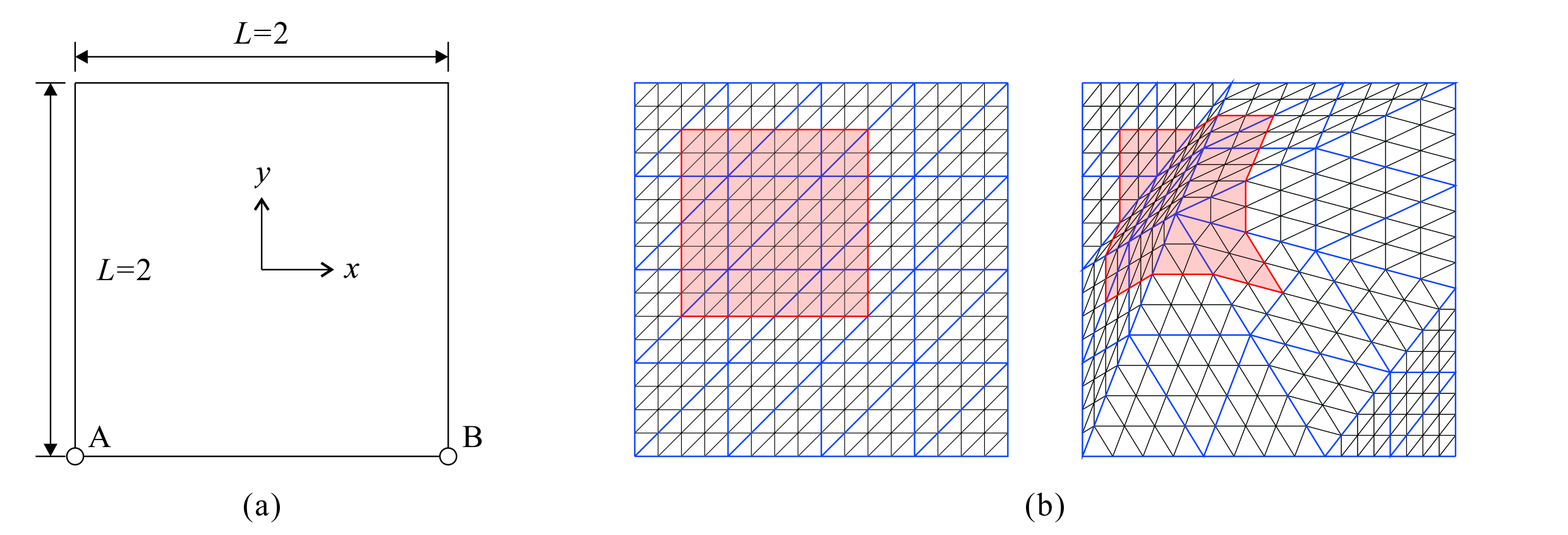
Figure 3: (a) Square domain $\Omega=(-1,1)^{2}\subset\mathbb{R}^{2}$ for the model Poisson and linear elasticity problems. (b) Domain decomposition settings for structured and unstructured meshes when $n=2^{4},N=2^{2}$, and $\delta=2h$. The blue and black lines represent the coarse and fine triangulations $\mathcal{T}_{H}$ and $\mathcal{T}_{h}$, respectively.

The first example is the Poisson problem (2.1) defined on the domain $\Omega=(-1,1)^{2}\subset\mathbb{R}^{2}$ shown in Fig. 3(a), where the function $f$ is given such that the problem has the exact solution $u(x,y)=e^{8(x+y)}\sin(\pi x)\sin(\pi y)$. The side length of the square domain $\Omega$ is denoted by $L=2$. We employ two types of coarse triangulations $\mathcal{T}_{H}$: the standard checkerboard type structured triangulation and an unstructured triangulation with nonuniform nodal points, with $2\times N\times N$ coarse elements ($N=2$, $2^{2}$, …, $2^{5}$). Fine triangulations $\mathcal{T}_{h}$ are constructed as the uniform refinements of $\mathcal{T}_{H}$ such that there are $2\times n\times n$ fine elements in the whole domain $\Omega$ ($n=2^{3}$, $2^{4}$, …, $2^{7}$). Each nonoverlapping subdomain $\Omega_{j}$, $1\leq j\leq\mathcal{N}=N\times N$, is a quadrilateral region composed of two coarse elements, and the corresponding overlapping subdomain $\Omega_{j}^{\prime}$ is formed by adding $\delta/h$ layers of fine elements; see Fig. 3(b) for the case of $n=2^{4}$ and $N=2^{2}$. The characteristic sizes of the fine and coarse meshes are calculated by $h=L/n$ and $H=L/N$, respectively. We set the overlap width $\delta$ as $h$ or $2h$, such that $\delta/h$ is constant.

				$n=2^{3}$		$n=2^{4}$		$n=2^{5}$		$n=2^{6}$		$n=2^{7}$
ES-FEM		Structured mesh		1.90e0		2.04e0		2.07e0		2.08e0		2.09e0
		Unstructured mesh		2.21e0		2.60e0		2.88e0		3.05e0		3.12e0
SSE		Structured mesh		2.87e0		3.24e0		3.34e0		3.37e0		3.38e0
		Unstructured mesh		3.45e0		4.32e0		4.90e0		5.26e0		5.40e0

Table 1: Condition numbers $\kappa(K^{-1}\bar{K}_{\mathrm{ES}})$ and $\kappa(K^{-1}\bar{K}_{\mathrm{SSE}})$ for the model Poisson problem (2.1).

Precond.	$N$		$n=2^{3}$			$n=2^{4}$			$n=2^{5}$			$n=2^{6}$			$n=2^{7}$
			#iter	$\kappa$		#iter	$\kappa$		#iter	$\kappa$		#iter	$\kappa$		#iter	$\kappa$
None			17	1.73e1		34	6.92e1		69	2.77e2		138	1.11e3		278	4.43e3
$M^{-1}$	$2$		13	5.73e0		14	6.67e0		13	6.41e0		14	7.99e0		15	1.52e1
	$2^{2}$		-	-		16	5.98e0		17	6.63e0		17	6.91e0		21	1.07e1
	$2^{3}$		-	-		-	-		16	5.86e0		18	6.72e0		19	7.00e0
	$2^{4}$		-	-		-	-		-	-		18	6.00e0		19	6.76e0
	$2^{5}$		-	-		-	-		-	-		-	-		18	6.04e0
$\bar{M}^{-1}$	$2$		9	4.81e0		9	5.58e0		10	6.84e0		11	1.00e1		12	1.76e1
	$2^{2}$		-	-		14	5.45e0		14	5.88e0		15	6.98e0		20	1.20e1
	$2^{3}$		-	-		-	-		15	5.49e0		15	5.91e0		17	7.00e0
	$2^{4}$		-	-		-	-		-	-		16	5.50e0		16	5.91e0
	$2^{5}$		-	-		-	-		-	-		-	-		16	5.45e0
$\bar{M}_{\mathrm{alt}}^{-1}$	$2$		9	4.75e0		9	5.62e0		9	6.88e0		11	1.00e1		12	1.76e1
	$2^{2}$		-	-		14	5.33e0		14	5.90e0		15	7.00e0		20	1.20e1
	$2^{3}$		-	-		-	-		15	5.37e0		15	5.95e0		16	7.00e0
	$2^{4}$		-	-		-	-		-	-		16	5.35e0		16	5.94e0
	$2^{5}$		-	-		-	-		-	-		-	-		16	5.24e0

Table 2: Condition numbers $\kappa$ and iteration counts #iter of the ES-FEM applied to the model Poisson problem (2.1) for the structured meshes and $\delta=2h$ with the two-level additive Schwarz preconditioners $M^{-1}$, $\bar{M}^{-1}$, and $\bar{M}_{\mathrm{alt}}^{-1}$ defined in (4.1), (4.2), and (4.3), respectively.

Precond.	$N$		$n=2^{3}$			$n=2^{4}$			$n=2^{5}$			$n=2^{6}$			$n=2^{7}$
			#iter	$\kappa$		#iter	$\kappa$		#iter	$\kappa$		#iter	$\kappa$		#iter	$\kappa$
None			15	1.32e1		30	5.22e1		59	2.08e2		119	8.30e2		240	3.32e3
$M^{-1}$	$2$		14	7.16e0		16	9.49e0		16	9.55e0		15	9.30e0		16	1.40e1
	$2^{2}$		-	-		18	7.62e0		20	9.53e0		20	1.01e1		21	1.01e1
	$2^{3}$		-	-		-	-		19	7.72e0		20	9.47e0		22	1.03e1
	$2^{4}$		-	-		-	-		-	-		20	7.55e0		22	9.59e0
	$2^{5}$		-	-		-	-		-	-		-	-		21	7.74e0
$\bar{M}^{-1}$	$2$		9	4.77e0		9	5.48e0		9	6.73e0		10	9.49e0		12	1.67e1
	$2^{2}$		-	-		14	5.42e0		14	5.77e0		15	6.87e0		20	1.18e1
	$2^{3}$		-	-		-	-		15	5.46e0		15	5.79e0		16	6.87e0
	$2^{4}$		-	-		-	-		-	-		16	5.46e0		16	5.79e0
	$2^{5}$		-	-		-	-		-	-		-	-		16	5.43e0
$\bar{M}_{\mathrm{alt}}^{-1}$	$2$		9	4.69e0		9	5.53e0		9	6.79e0		10	9.49e0		12	1.67e1
	$2^{2}$		-	-		14	5.27e0		14	5.80e0		15	6.90e0		20	1.18e1
	$2^{3}$		-	-		-	-		15	5.30e0		15	5.85e0		16	6.88e0
	$2^{4}$		-	-		-	-		-	-		16	5.29e0		16	5.84e0
	$2^{5}$		-	-		-	-		-	-		-	-		16	5.23e0

Table 3: Condition numbers $\kappa$ and iteration counts #iter of the SSE applied to the model Poisson problem (2.1) for the structured meshes and $\delta=2h$ with the two-level additive Schwarz preconditioners $M^{-1}$, $\bar{M}^{-1}$, and $\bar{M}_{\mathrm{alt}}^{-1}$ defined in (4.1), (4.2), and (4.3), respectively.

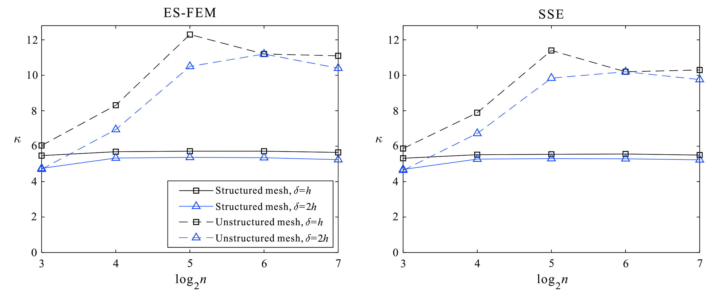
Figure 4: Condition numbers $\kappa(\bar{M}_{\mathrm{alt}}^{-1}\bar{K})$ of the ES-FEM and SSE applied to the model Poisson problem (2.1) when $n$ varies and $n/N$ $(=H/h)$ is fixed as $4$.

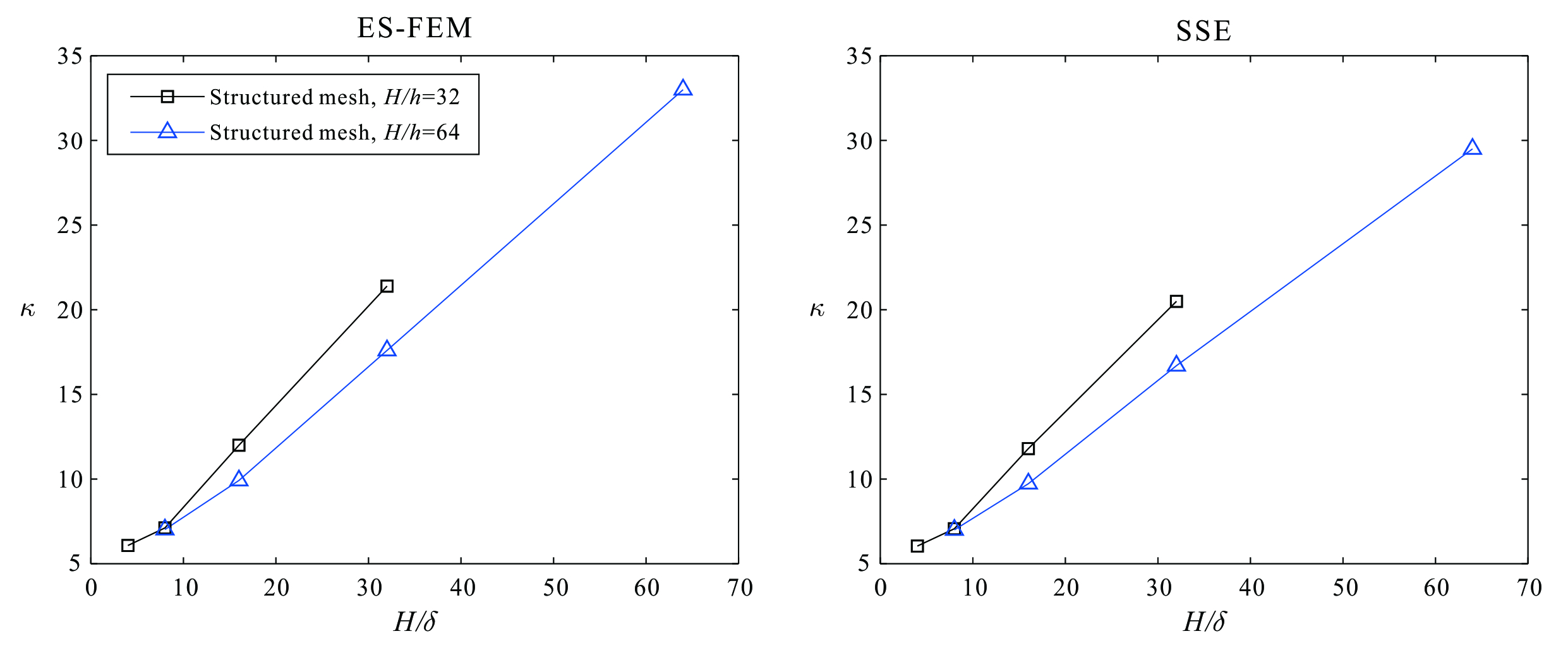
Figure 5: Condition numbers $\kappa(\bar{M}_{\mathrm{alt}}^{-1}\bar{K})$ of the ES-FEM and SSE applied to the model Poisson problem (2.1) when $H/\delta$ varies and $n/N$ $(=H/h)$ is fixed as $32$ or $64$.

Table 1 provides the condition numbers $\kappa(K^{-1}\bar{K}_{\mathrm{ES}})$ and $\kappa(K^{-1}\bar{K}_{\mathrm{SSE}})$ for the structured and unstructured meshes for various values of $n$. The condition numbers $\kappa(K^{-1}\bar{K}_{\mathrm{ES}})$ and $\kappa(K^{-1}\bar{K}_{\mathrm{SSE}})$ are eventually bounded when $n$ increases. Hence, the stiffness matrices $\bar{K}_{\mathrm{ES}}$ and $\bar{K}_{\mathrm{SSE}}$ of the ES-FEM and SSE, respectively, are spectrally equivalent to the stiffness matrix $K$ of the standard FEM. This numerically verifies Theorems 3.2 and 3.4. Tables 2 and 3 exhibit the condition numbers of the $M^{-1}$-, $\bar{M}^{-1}$-, and $\bar{M}_{\mathrm{alt}}^{-1}$-preconditioned stiffness matrices of the ES-FEM and SSE, respectively, and the corresponding conjugate gradient iteration counts denoted as #iter for the structured meshes with various values of $n$ and $N$. Fig. 4 depicts the condition numbers of the $\bar{M}_{\mathrm{alt}}^{-1}$-preconditioned ES-FEM and SSE for the structured and unstructured meshes when $n/N$ $(=H/h)$ is fixed as $4$. As we have explained theoretically in Section 4, $M^{-1}$-, $\bar{M}^{-1}$-, and $\bar{M}_{\mathrm{alt}}^{-1}$-preconditioned ES-FEM and SSE are all numerically scalable in the sense that the condition number and iteration count are eventually bounded when $n$ and $N$ increase keeping $n/N$ constant. Moreover, we observe that each iteration count for the preconditioner $\bar{M}^{-1}$ is less than the corresponding counterpart for the preconditioner $M^{-1}$, which numerically verifies Theorem 4.3. We also highlight that the condition numbers and iteration counts for the preconditioner $\bar{M}_{\mathrm{alt}}^{-1}$ are comparable to those for $\bar{M}^{-1}$. Hence, as we have claimed in Section 4, $\bar{M}_{\mathrm{alt}}^{-1}$ can be a good alternative to $\bar{M}^{-1}$ with a comparable performance and easy implementation. In addition, Fig. 5 provides the condition numbers of the $\bar{M}_{\mathrm{alt}}^{-1}$-preconditioned ES-FEM and SSE for the structured meshes when $H/\delta$ varies and $n/N$ $(=H/h)$ is fixed as $32$ or $64$. We verify the linear growth of the condition numbers for increasing values of $H/\delta$.

5.2 Linear elasticity

We consider the following model linear elasticity problem defined on the domain $\Omega=(-1,1)^{2}\subset\mathbb{R}^{2}$:

$$-\operatorname{div}\sigma(u)=b\hskip 2.84544pt\textrm{ in }\Omega,$$ (5.1)

where $\sigma(u)$ is the Cauchy stress, $b$ is the body force given by $b(x,y)=(-y^{2},1-x^{2})$, and the Dirichlet boundary condition $u=0$ is given along line AB (see Fig. 3(a)). The plane stress condition is employed with Young’s modulus $E=1\times 10^{3}$ and Poisson’s ratio $\nu=0.2$. The finite element models are constructed using $2\times n\times n$ fine elements ($n=2^{3}$, $2^{4}$, …, $2^{7}$) and $2\times N\times N$ coarse elements ($N=2$, $2^{2}$, …, $2^{5}$) with the overlap width $\delta=h$ or $2h$, as shown in Fig. 3(b). We only present the results for the structured meshes; as in the case of the Poisson’s equation, the unstructured meshes show similar behaviors as the structured meshes.

		$n=2^{3}$		$n=2^{4}$		$n=2^{5}$		$n=2^{6}$		$n=2^{7}$
ES-FEM		2.27e0		2.30e0		2.32e0		2.33e0		2.33e0
SSE		3.68e0		3.78e0		3.84e0		3.86e0		3.87e0

Table 4: Condition numbers $\kappa(K^{-1}\bar{K}_{\mathrm{ES}})$ and $\kappa(K^{-1}\bar{K}_{\mathrm{SSE}})$ with the structured meshes for the model linear elasticity problem (5.1).

Precond.	$N$		$n=2^{3}$			$n=2^{4}$			$n=2^{5}$			$n=2^{6}$			$n=2^{7}$
			#iter	$\kappa$		#iter	$\kappa$		#iter	$\kappa$		#iter	$\kappa$		#iter	$\kappa$
None			71	1.05e3		139	3.71e3		272	1.38e4		535	5.32e4		1065	2.08e5
$M^{-1}$	$2$		21	8.80e0		22	9.73e0		24	1.16e1		30	1.76e1		40	3.14e1
	$2^{2}$		-	-		23	8.96e0		25	9.20e0		28	1.17e1		37	2.01e1
	$2^{3}$		-	-		-	-		23	8.33e0		25	9.20e0		28	1.19e1
	$2^{4}$		-	-		-	-		-	-		23	8.24e0		25	9.32e0
	$2^{5}$		-	-		-	-		-	-		-	-		23	8.16e0
$\bar{M}^{-1}$	$2$		18	7.66e0		20	9.26e0		22	1.22e1		28	1.94e1		38	3.51e1
	$2^{2}$		-	-		20	6.88e0		21	7.58e0		26	1.18e1		33	2.13e1
	$2^{3}$		-	-		-	-		20	6.83e0		22	8.58e0		26	1.19e1
	$2^{4}$		-	-		-	-		-	-		20	6.72e0		22	8.78e0
	$2^{5}$		-	-		-	-		-	-		-	-		20	6.71e0
$\bar{M}_{\mathrm{alt}}^{-1}$	$2$		18	8.52e0		20	1.00e1		24	1.26e1		29	1.95e1		39	3.52e1
	$2^{2}$		-	-		21	7.77e0		23	9.25e0		28	1.24e1		36	2.17e1
	$2^{3}$		-	-		-	-		21	7.63e0		23	9.23e0		28	1.25e1
	$2^{4}$		-	-		-	-		-	-		21	7.60e0		24	9.50e0
	$2^{5}$		-	-		-	-		-	-		-	-		21	7.61e0

Table 5: Condition numbers $\kappa$ and iteration counts #iter of the ES-FEM applied to the model linear elasticity problem (5.1) for the structured meshes and $\delta=2h$ with the two-level additive Schwarz preconditioners $M^{-1}$, $\bar{M}^{-1}$, and $\bar{M}_{\mathrm{alt}}^{-1}$ defined in (4.1), (4.2), and (4.3), respectively.

Precond.	$N$		$n=2^{3}$			$n=2^{4}$			$n=2^{5}$			$n=2^{6}$			$n=2^{7}$
			#iter	$\kappa$		#iter	$\kappa$		#iter	$\kappa$		#iter	$\kappa$		#iter	$\kappa$
None			67	8.00e2		123	2.80e3		237	1.04e4		464	3.99e4		922	1.56e5
$M^{-1}$	$2$		24	1.29e1		26	1.23e1		28	1.28e1		30	1.70e1		38	3.03e1
	$2^{2}$		-	-		27	1.43e1		28	1.32e1		29	1.36e1		36	1.96e1
	$2^{3}$		-	-		-	-		27	1.41e1		29	1.35e1		30	1.39e1
	$2^{4}$		-	-		-	-		-	-		27	1.33e1		30	1.36e1
	$2^{5}$		-	-		-	-		-	-		-	-		26	1.11e1
$\bar{M}^{-1}$	$2$		18	7.45e0		19	9.02e0		22	1.20e1		28	1.90e1		36	3.43e1
	$2^{2}$		-	-		20	6.76e0		21	7.34e0		25	1.15e1		33	2.08e1
	$2^{3}$		-	-		-	-		20	6.67e0		22	8.35e0		25	1.16e1
	$2^{4}$		-	-		-	-		-	-		20	6.55e0		22	8.55e0
	$2^{5}$		-	-		-	-		-	-		-	-		20	6.54e0
$\bar{M}_{\mathrm{alt}}^{-1}$	$2$		18	8.33e0		20	9.82e0		23	1.24e1		29	1.91e1		37	3.44e1
	$2^{2}$		-	-		21	7.56e0		23	9.00e0		27	1.21e1		35	2.11e1
	$2^{3}$		-	-		-	-		21	7.25e0		23	8.99e0		27	1.22e1
	$2^{4}$		-	-		-	-		-	-		21	7.31e0		23	9.19e0
	$2^{5}$		-	-		-	-		-	-		-	-		21	7.32e0

Table 6: Condition numbers $\kappa$ and iteration counts #iter of the SSE applied to the model linear elasticity problem (5.1) for the structured meshes and $\delta=2h$ with the two-level additive Schwarz preconditioners $M^{-1}$, $\bar{M}^{-1}$, and $\bar{M}_{\mathrm{alt}}^{-1}$ defined in (4.1), (4.2), and (4.3), respectively.

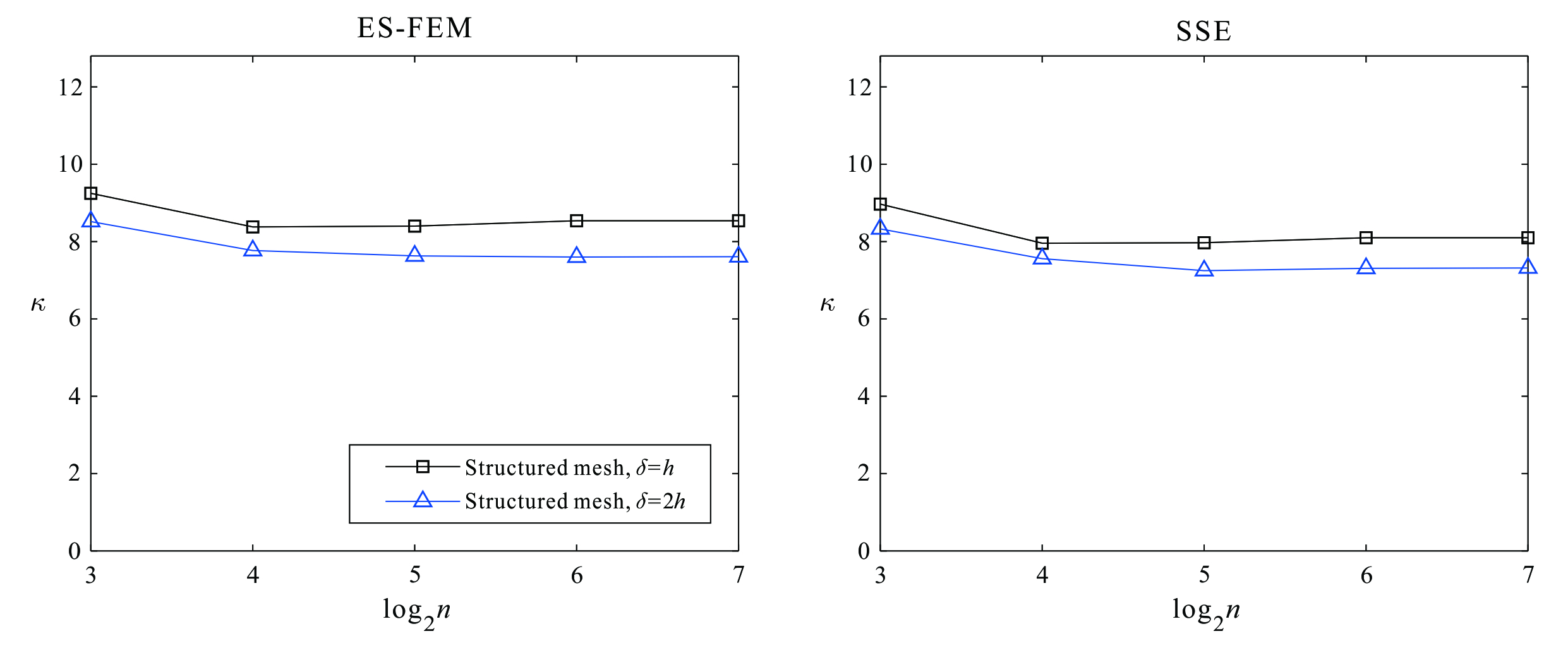
Figure 6: Condition numbers $\kappa(\bar{M}_{\mathrm{alt}}^{-1}\bar{K})$ of the ES-FEM and SSE applied to the model linear elasticity problem (5.1) for the structured meshes when $n$ varies and $n/N$ $(=H/h)$ is fixed as $4$.

Table 4 provides the condition numbers $\kappa(K^{-1}\bar{K}_{\mathrm{ES}})$ and $\kappa(K^{-1}\bar{K}_{\mathrm{SSE}})$ for various $n$. Since the condition numbers for both ES-FEM and SSE are eventually bounded when $n$ becomes larger, we confirm the spectral equivalence among the stiffness matrices of the standard FEM, ES-FEM, and SSE. Table 5 presents the condition numbers of the $M^{-1}$-, $\bar{M}^{-1}$-, and $\bar{M}_{\mathrm{alt}}^{-1}$-preconditioned stiffness matrices and the corresponding conjugate gradient iteration counts #iter for the ES-FEM. Table 6 presents the results corresponding to the SSE. Fig. 6 shows the condition numbers when the preconditioner $\bar{M}_{\mathrm{alt}}^{-1}$ is used and $n/N$ $(=H/h)$ is fixed as $4$ for the ES-FEM and SSE. Similar to the Poisson problem, it is observed that both the condition number and iteration count are eventually bounded when $n$ and $N$ increase, keeping the ratio $n/N$ constant, which implies that all the preconditioned methods are numerically scalable. Moreover, the iteration counts for the preconditioners $\bar{M}^{-1}$ and $\bar{M}_{\mathrm{alt}}^{-1}$ are smaller than the corresponding values for $M^{-1}$ for most of the cases; this indicates the numerical efficiency of the proposed enhanced preconditioners $\bar{M}^{-1}$ and $\bar{M}_{\mathrm{alt}}^{-1}$ applied to the linear elasticity problem. In conclusion, we have numerically proven that all the theoretical results developed in this study are valid for the Poisson and linear elasticity problems.

6 Remarks on node-based strain smoothing

We observed that the ES-FEM and SSE enjoy the spectral equivalence with the standard FEM. In contrast, not every FEM with strain smoothing satisfies such equivalence property. Particularly, we present an example in which the stiffness matrix of the NS-FEM may not be spectrally equivalent to that of the standard FEM.

In the NS-FEM, each element in $\mathcal{T}_{h}$ is divided into three quadrilateral subdomains using its nodes, midpoints of element edges, and barycenter. The node-based smoothing domains consist of assemblages of adjacent subdomains belonging to different elements based on nodes; see Fig. 1(c). Denoting the collection of all smoothing domains constructed from $\mathcal{T}_{h}$ for the NS-FEM by $\mathcal{S}_{h,\mathrm{NS}}$, a smoothed gradient $\bar{\epsilon}^{(s)}$ for a smoothing domain $s\in\mathcal{S}_{h,\mathrm{NS}}$ is defined by

$$\bar{\epsilon}^{(s)}=\frac{\sum_{k=1}^{m}|e^{(k)}|\epsilon^{(e^{(k)})}}{\sum_{k=1}^{m}|e^{(k)}|},$$ (6.1)

where $e^{(k)}$ is the $k$th element in $\mathcal{T}_{h}$ neighboring to the node corresponding to $s$, $\epsilon^{(e^{(k)})}$ was defined in (2.2), and $m$ is the number of neighboring elements in $\mathcal{T}_{h}$. The number $m$ varies per node in general. Using the smoothed gradient in (6.1), the stiffness matrix $\bar{K}_{\mathrm{NS}}$ for the NS-FEM is defined in a similar manner as (2.7). It is known that the NS-FEM is effective in alleviating volumetric locking [3].

The following example shows that the NS-FEM in one-dimension is not spectrally equivalent to the standard FEM; examples corresponding to higher-dimensional cases can be constructed similarly.

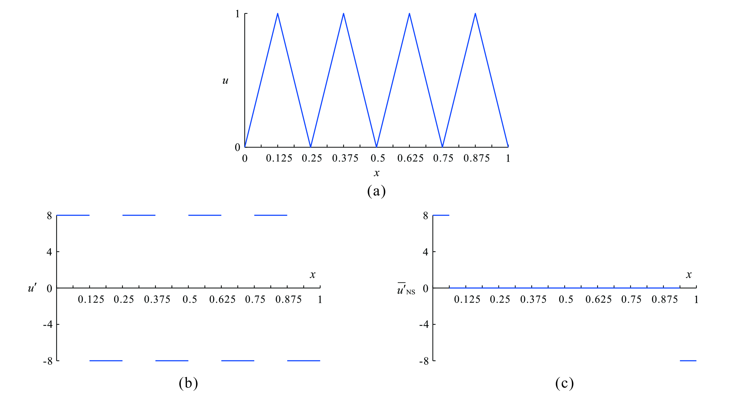
Figure 7: Graphs of (a) the function $u$, (b) its derivative $u^{\prime}$, and (c) the node-based smoothed derivative $\bar{u^{\prime}}_{\mathrm{NS}}$ in Example 6.1, when $n=8$.

Figure 8: Graphs of (a) the function $v$, (b) its derivative $v^{\prime}$, and (c) the node-based smoothed derivative $\bar{v^{\prime}}_{\mathrm{NS}}$ in Example 6.1, when $n=8$.

Example 6.1.

Let $\Omega=[0,1]\subset\mathbb{R}$ and let $\mathcal{T}_{h}$ be the uniform partition of $\Omega$ into $n$ subintervals, where $n$ is a positive even integer. In this case, the space $V_{h}$ is defined as the collection of all piecewise linear and continuous functions on $\mathcal{T}_{h}$ satisfying the homogeneous Dirichlet boundary condition. As depicted in Fig. 7(a), we set $u\in V_{h}$ such that

$$u\left(\frac{i}{n}\right)=\begin{cases}0&\text{ if }i\text{ is even},\\ 1&\text{ if }i\text{ is odd},\end{cases}\quad i=1,2,\dots,n-1.$$

In each subinterval $i/n<x<(i+1)/n$, $i=0,1,\dots,n-1$, we have

$$u^{\prime}(x)=\begin{cases}n&\text{ if }i\text{ is even},\\ -n&\text{ if }i\text{ is odd}.\end{cases}$$

By applying the node-based smoothing to $u^{\prime}$, we obtain the smoothed derivative $\bar{u^{\prime}}_{\mathrm{NS}}$ as follows:

$$\bar{u^{\prime}}_{\mathrm{NS}}(x)=\begin{cases}n&\text{ if }0<x<\frac{1}{2n},\\ 0&\text{ if }\frac{1}{2n}<x<1-\frac{1}{2n},\\ -n&\textrm{ if }1-\frac{1}{2n}<x<1.\end{cases}$$

The graphs of $u^{\prime}$ and $\bar{u^{\prime}}_{\mathrm{NS}}$ are plotted in Figs. 7(b) and (c), respectively. Hence, it follows that

$$\lambda_{\min}(K^{-1}\bar{K}_{\mathrm{NS}})\leq\frac{u^{T}\bar{K}_{\mathrm{NS}}u}{u^{T}Ku}=\frac{\int_{\Omega}|\bar{u^{\prime}}_{\mathrm{NS}}|^{2}\,dx}{\int_{\Omega}|u^{\prime}|^{2}\,dx}=\frac{1}{n}.$$ (6.2)

Meanwhile, as shown in Fig. 8(a), we set $v\in V_{h}$ such that

$$v\left(\frac{i}{n}\right)=1,\quad i=1,2,\dots,n-1.$$

Then one can readily obtain

$$v^{\prime}(x)=\begin{cases}n&\text{ if }0<x<\frac{1}{n},\\ 0&\text{ if }\frac{1}{n}<x<1-\frac{1}{n},\\ -n&\textrm{ if }1-\frac{1}{n}<x<1,\end{cases}$$

and

$$\bar{v^{\prime}}_{\mathrm{NS}}(x)=\begin{cases}n&\text{ if }0<x<\frac{1}{2n},\\ \frac{n}{2}&\text{ if }\frac{1}{2n}<x<\frac{3}{2n},\\ 0&\text{ if }\frac{3}{2n}<x<1-\frac{3}{2n},\\ -\frac{n}{2}&\text{ if }1-\frac{3}{2n}<x<1-\frac{1}{2n},\\ -n&\textrm{ if }1-\frac{1}{2n}<x<1.\end{cases}$$

See Figs. 8(b) and (c) for the graphs of $v^{\prime}$ and $\bar{v^{\prime}}_{\mathrm{NS}}$, respectively. By direct calculation, we have

$$\lambda_{\max}(K^{-1}\bar{K}_{\mathrm{NS}})\geq\frac{v^{T}\bar{K}_{\mathrm{NS}}v}{v^{T}Kv}=\frac{\int_{\Omega}|\bar{v^{\prime}}_{\mathrm{NS}}|^{2}\,dx}{\int_{\Omega}|v^{\prime}|^{2}\,dx}=\frac{3}{4}.$$ (6.3)

Combining (6.2) and (6.3) yields

$$\kappa(K^{-1}\bar{K}_{\mathrm{NS}})=\frac{\lambda_{\max}(K^{-1}\bar{K}_{\mathrm{NS}})}{\lambda_{\min}(K^{-1}\bar{K}_{\mathrm{NS}})}\geq\frac{3n}{4}=O(h^{-1}),$$

which implies that $\bar{K}_{\mathrm{NS}}$ and $K$ are not spectrally equivalent.

		$n=2^{3}$		$n=2^{4}$		$n=2^{5}$		$n=2^{6}$		$n=2^{7}$
NS-FEM		9.36e1		3.75e2		1.53e3		6.21e3		2.50e4

Table 7: Condition numbers $\kappa(K^{-1}\bar{K}_{\mathrm{NS}})$ with the structured meshes for the model linear elasticity problem (5.1).

Precond.	$N$		$n=2^{3}$			$n=2^{4}$			$n=2^{5}$			$n=2^{6}$			$n=2^{7}$
			#iter	$\kappa$		#iter	$\kappa$		#iter	$\kappa$		#iter	$\kappa$		#iter	$\kappa$
None			60	4.03e2		112	1.40e3		204	5.19e3		393	1.99e4		743	7.81e4
$M^{-1}$	$2$		60	1.22e2		133	7.81e2		270	3.87e3		498	1.77e4		906	7.62e4
	$2^{2}$		-	-		116	4.47e2		269	3.26e3		515	1.58e4		943	6.54e4
	$2^{3}$		-	-		-	-		218	1.82e3		496	1.30e4		963	6.24e4
	$2^{4}$		-	-		-	-		-	-		389	7.25e3		906	5.14e4
	$2^{5}$		-	-		-	-		-	-		-	-		694	2.69e4
$\bar{M}^{-1}$	$2$		18	6.94e0		23	1.07e1		31	2.12e1		44	4.37e1		62	8.98e1
	$2^{2}$		-	-		29	1.80e1		37	3.70e1		54	8.23e1		78	1.76e2
	$2^{3}$		-	-		-	-		52	6.82e1		66	1.48e2		97	3.40e2
	$2^{4}$		-	-		-	-		-	-		95	2.74e2		119	6.03e2
	$2^{5}$		-	-		-	-		-	-		-	-		172	1.11e3
$\bar{M}_{\mathrm{alt}}^{-1}$	$2$		18	7.85e0		24	1.10e1		32	2.16e1		45	4.39e1		63	8.99e1
	$2^{2}$		-	-		29	1.82e1		38	3.97e1		56	8.57e1		80	1.78e2
	$2^{3}$		-	-		-	-		52	6.93e1		69	1.62e2		102	3.59e2
	$2^{4}$		-	-		-	-		-	-		96	2.80e2		125	6.63e2
	$2^{5}$		-	-		-	-		-	-		-	-		173	1.13e3

Table 8: Condition numbers $\kappa$ and iteration counts #iter of the NS-FEM applied to the model linear elasticity problem (5.1) for the structured meshes and $\delta=2h$ with the two-level additive Schwarz preconditioners $M^{-1}$, $\bar{M}^{-1}$, and $\bar{M}_{\mathrm{alt}}^{-1}$ defined in (4.1), (4.2), and (4.3), respectively.

We revisit the linear elasticity problem in Section 5.2 using the structured meshes, as shown in Fig. 3; Table 7 provides the condition numbers $\kappa(K^{-1}\bar{K}_{\mathrm{NS}})$ for various values of $n$. The results show that the stiffness matrix of the NS-FEM is not spectrally equivalent to that of the standard FEM; $\kappa(K^{-1}\bar{K}_{\mathrm{NS}})$ increases approximately four times whenever $n$ doubles. Table 8 presents the condition numbers of the $M^{-1}$-, $\bar{M}^{-1}$-, and $\bar{M}_{\mathrm{alt}}^{-1}$-preconditioned stiffness matrices and the corresponding conjugate gradient iteration counts #iter for the NS-FEM. As expected, the condition number and iteration count increase when $n$ and $N$ increase, keeping the ratio $n/N$ constant for all the preconditioners considered. Additionally, it is numerically confirmed that the preconditioners $\bar{M}^{-1}$ and $\bar{M}_{\mathrm{alt}}^{-1}$ reduce the condition number to some extent, whereas the preconditioner $M^{-1}$ does not.

7 Conclusion

Based on the fact that the stiffness matrices of the standard FEM, ES-FEM, and SSE are spectrally equivalent, we proved that any existing preconditioner for the standard FEM can be applied to the ES-FEM and SSE, inheriting good convergence properties such as numerical scalability. We proposed the improved two-level additive Schwarz preconditioners for the ES-FEM and SSE. Theoretically and numerically, the proposed preconditioners outperformed the standard one when they were applied to the ES-FEM and SSE.

This study suggests several interesting topics for future research. The motivation for developing iterative solvers may influence their application to large-scale problems; we must solve more complex engineering problems on a large scale using FEMs with strain smoothing, equipped with the proposed preconditioners. It is interesting to consider large-scale problems with oscillatory and high contrast coefficients [34, 35], which appear in the mathematical modeling of the flow in heterogeneous porous media. Meanwhile, we observed in Section 6 that the spectral property of the NS-FEM is different from the ES-FEM and SSE. This proves that mathematical properties of the NS-FEM are somewhat different from those of other FEMs with strain smoothing. Hence, developing a mathematical theory on the NS-FEM should be considered as a separate study.

Appendix A Convergence theory of additive Schwarz methods

In this appendix, we provide a brief summary on the abstract convergence theory of additive Schwarz methods introduced in [23, 33]. Let $V$ be a Hilbert space. We consider the model linear problem

$$Au=f,$$

where $A\colon V\rightarrow V$ is a symmetric and positive definite linear operator and $f\in V$. In what follows, an index $j$ runs from $1$ to $\mathcal{N}$. For a Hilbert space $V_{j}$, we assume that there exists an interpolation operator $R_{j}^{T}\colon V_{j}\rightarrow V$ such that $V=\sum_{j=1}^{\mathcal{N}}R_{j}^{T}V_{j}$. Let $\tilde{A}_{j}\colon V_{j}\rightarrow V_{j}$ be a symmetric and positive definite linear operator which plays a role of a local operator on $V_{j}$. In this setting, the additive Schwarz preconditioner $M^{-1}\colon V\rightarrow V$ is given by

$$M^{-1}=\sum_{j=1}^{\mathcal{N}}R_{j}^{T}\tilde{A}_{j}^{-1}R_{j}.$$

In order to obtain an upper bound for the condition number of the preconditioned operator $M^{-1}A$, we need the following three assumptions [33, Assumptions 4.9–4.11].

Assumption A.1.

There exists a constant $C_{0}>0$ which satisfies the following: for any $v\in V$, there exists $v_{j}\in V_{j}$, $1\leq j\leq\mathcal{N}$, such that

$$v=\sum_{j=1}^{\mathcal{N}}R_{j}^{T}v_{j}$$

and

$$\sum_{j=1}^{\mathcal{N}}v_{j}^{T}\tilde{A}_{j}v_{j}\leq C_{0}^{2}v^{T}Av.$$

Assumption A.2.

There exists a constant $\tau_{0}>0$ which satisfies the following: for any $v_{j}\in V_{j}$, $1\leq j\leq\mathcal{N}$, and $\tau\in(0,\tau_{0}]$, we have

$$\left(\sum_{j=1}^{\mathcal{N}}R_{j}^{T}v_{j}\right)^{T}A\left(\sum_{j=1}^{\mathcal{N}}R_{j}^{T}v_{j}\right)\leq\frac{1}{\tau}\sum_{j=1}^{\mathcal{N}}(R_{j}^{T}v_{j})^{T}A(R_{j}v_{j}).$$

Assumption A.3.

There exists a constant $\omega_{0}>0$ which satisfies the following: for any $v_{j}\in V_{j}$, $1\leq j\leq\mathcal{N}$, we have

$$(R_{j}^{T}v_{j})^{T}A(R_{j}^{T}v_{j})\leq\omega_{0}v_{j}^{T}\tilde{A}_{j}v_{j}.$$

For detailed explanations of the assumptions above, we refer to [23, 33]. Under Assumptions A.1, A.2, and A.3, we define the additive Schwarz condition number $\kappa_{\mathrm{ASM}}$ as follows:

$$\kappa_{\mathrm{ASM}}=\frac{\omega_{0}C_{0}^{2}}{\tau_{0}},$$ (A.1)

where $C_{0}$, $\tau_{0}$, and $\omega_{0}$ are chosen as optimal as possible. That is, $C_{0}$ is chosen as the minimum one satisfying Assumption A.1, $\tau_{0}$ as the maximum one satisfying Assumption A.2, and $\omega_{0}$ as the minimum one satisfying Assumption A.3. The following theorem suggests that the convergence rate of a preconditioned iterative algorithm for $M^{-1}A$ relies on the additive Schwarz condition number $\kappa_{\mathrm{ASM}}$ [33].

Theorem A.4.

Under Assumptions A.1, A.2, and A.3, we have

$$\frac{\tau_{0}}{\omega_{0}}v^{T}Av\leq v^{T}Mv\leq C_{0}^{2}v^{T}Av\quad\forall v\in V.$$

Consequently, the following holds:

$$\kappa(M^{-1}A)\leq\kappa_{\mathrm{ASM}},$$

where $\kappa_{\mathrm{ASM}}$ was given in (A.1).

References

- Chen et al. [2001] J. S. Chen, C. T. Wu, S. Yoon, Y. Y, A stabilized conforming nodal integration for Galerkin mesh-free methods, International Journal for Numerical Methods in Engineering 50 (2001) 435–466.
- Liu et al. [2007] G. R. Liu, K. Y. Dai, T. T. Nguyen, A smoothed finite element method for mechanics problems, Computational Mechanics 39 (2007) 859–877.
- Liu et al. [2009a] G. R. Liu, T. Nguyen-Thoi, H. Nguyen-Xuan, K. Y. Lam, A node-based smoothed finite element method (NS-FEM) for upper bound solutions to solid mechanics problems, Computers & Structures 87 (2009a) 14–26.
- Liu et al. [2009b] G. R. Liu, T. Nguyen-Thoi, K. Y. Lam, An edge-based smoothed finite element method (ES-FEM) for static, free and forced vibration analyses of solids, Journal of Sound and Vibration 320 (2009b) 1100–1130.
- Liu and Nguyen-Thoi [2010] G. R. Liu, T. Nguyen-Thoi, Smoothed Finite Element Methods, CRC Press, New York, 2010.
- Hamrani et al. [2017] A. Hamrani, S. H. Habib, I. Belaidi, CS-IGA: A new cell-based smoothed isogeometric analysis for 2D computational mechanics problems, Computer Methods in Applied Mechanics and Engineering 315 (2017) 671–690.
- Yuan et al. [2019] W. H. Yuan, B. Wang, W. Zhang, Q. Jiang, X. T. Feng, Development of an explicit smoothed particle finite element method for geotechnical applications, Computers and Geotechnics 106 (2019) 42–51.
- Nguyen-Xuan et al. [2008] H. Nguyen-Xuan, S. Bordas, H. Nguyen-Dang, Smooth finite element methods: convergence, accuracy and properties, International Journal for Numerical Methods in Engineering 74 (2008) 175–208.
- Liu et al. [2010] G. R. Liu, H. Nguyen-Xuan, T. Nguyen-Thoi, A theoretical study on the smoothed FEM (S-FEM) models: Properties, accuracy and convergence rates, International Journal for Numerical Methods in Engineering 84 (2010) 1222–1256.
- Lee and Lee [2018] C. Lee, P. S. Lee, A new strain smoothing method for triangular and tetrahedral finite elements, Computer Methods in Applied Mechanics and Engineering 341 (2018) 939–955.
- Lee and Lee [2019] C. Lee, P. S. Lee, The strain-smoothed MITC3+ shell finite element, Computers & Structures 223 (2019) 106096.
- Lee et al. [2021] C. Lee, S. Kim, P. S. Lee, The strain-smoothed 4-node quadrilateral finite element, Computer Methods in Applied Mechanics and Engineering 373 (2021) 113481.
- Lee et al. [2022a] C. Lee, M. Moon, J. Park, A gradient smoothing method and its multiscale variant for flows in heterogeneous porous media, Computer Methods in Applied Mechanics and Engineering 395 (2022a) 115039.
- Lee et al. [2022b] C. Lee, D.-H. Lee, P. S. Lee, The strain-smoothed MITC3+ shell element in nonlinear analysis, Computers & Structures 265 (2022b) 106768.
- Lee and Park [2021] C. Lee, J. Park, A variational framework for the strain-smoothed element method, Computers & Mathematics with Applications 94 (2021) 76–93.
- Zeng and Liu [2018] W. Zeng, G. Liu, Smoothed finite element methods (S-FEM): an overview and recent developments, Archives of Computational Methods in Engineering 25 (2018) 397–435.
- Farhat and Roux [1994] C. Farhat, F.-X. Roux, Implicit parallel processing in structural mechanics, Computational Mechanics Advances 2 (1994) 1–124.
- Saad [2003] Y. Saad, Iterative Methods for Sparse Linear Systems, SIAM, Philadelphia, 2003.
- Smith [1992] B. F. Smith, An optimal domain decomposition preconditioner for the finite element solution of linear elasticity problems, SIAM Journal on Scientific and Statistical Computing 13 (1992) 364–378.
- Klawonn and Pavarino [1998] A. Klawonn, L. F. Pavarino, Overlapping Schwarz methods for mixed linear elasticity and Stokes problems, Computer Methods in Applied Mechanics and Engineering 165 (1998) 233–245.
- Griebel et al. [2003] M. Griebel, D. Oeltz, M. A. Schweitzer, An algebraic multigrid method for linear elasticity, SIAM Journal on Scientific Computing 25 (2003) 385–407.
- Dohrmann and Widlund [2009] C. R. Dohrmann, O. B. Widlund, An overlapping Schwarz algorithm for almost incompressible elasticity, SIAM Journal on Numerical Analysis 47 (2009) 2897–2923.
- Toselli and Widlund [2005] A. Toselli, O. Widlund, Domain Decomposition Methods—Algorithms and Theory, Springer, Berlin, 2005.
- Da Veiga et al. [2013] L. B. Da Veiga, D. Cho, L. Pavarino, S. Scacchi, Isogeometric Schwarz preconditioners for linear elasticity systems, Computer Methods in Applied Mechanics and Engineering 253 (2013) 439–454.
- Calvo [2019] J. G. Calvo, An overlapping Schwarz method for virtual element discretizations in two dimensions, Computers & Mathematics with Applications 77 (2019) 1163–1177.
- Cho et al. [2021] D. Cho, L. Pavarino, S. Scacchi, Overlapping additive Schwarz preconditioners for isogeometric collocation discretizations of linear elasticity, Computers & Mathematics with Applications 93 (2021) 66–77.
- Xu [1992] J. Xu, Iterative methods by space decomposition and subspace correction, SIAM Review 34 (1992) 581–613.
- Xu [2001] J. Xu, The method of subspace corrections, Journal of Computational and Applied Mathematics 128 (2001) 335–362.
- Nguyen-Thoi et al. [2011] T. Nguyen-Thoi, G. R. Liu, H. Nguyen-Xuan, An n-sided polygonal edge-based smoothed finite element method (nES-FEM) for solid mechanics, International Journal for Numerical Methods in Biomedical Engineering 27 (2011) 1446–1472.
- Ciarlet [2002] P. G. Ciarlet, The Finite Element Method for Elliptic Problems, SIAM, Philadelphia, 2002.
- Brenner and Scott [2008] S. Brenner, R. Scott, The Mathematical Theory of Finite Element Methods, Springer, New York, 2008.
- Liu [2010] G. R. Liu, A G space theory and a weakened weak (W2) form for a unified formulation of compatible and incompatible methods: Part I theory, International Journal for Numerical Methods in Engineering 81 (2010) 1093–1126.
- Park [2020] J. Park, Additive Schwarz methods for convex optimization as gradient methods, SIAM Journal on Numerical Analysis 58 (2020) 1495–1530.
- Klawonn et al. [2015] A. Klawonn, P. Radtke, O. Rheinbach, FETI-DP methods with an adaptive coarse space, SIAM Journal on Numerical Analysis 53 (2015) 297–320.
- Kim et al. [2017] H. H. Kim, E. Chung, J. Wang, BDDC and FETI-DP preconditioners with adaptive coarse spaces for three-dimensional elliptic problems with oscillatory and high contrast coefficients, Journal of Computational Physics 349 (2017) 191–214.