A parallel-in-time preconditioner for Crank-Nicolson discretization of a parabolic optimal control problem

Abstract

In this paper, a fast solver is studied for saddle point system arising from a second-order Crank-Nicolson discretization of an initial-valued parabolic PDE constrained optimal control problem, which is indefinite and ill-conditioned. Different from the saddle point system arising from the first-order Euler discretization, the saddle point system arising from Crank-Nicolson discretization has a dense and non-symmetric Schur complement, which brings challenges to fast solver designing. To remedy this, a novel symmetrization technique is applied to the saddle point system so that the new Schur complement is symmetric definite and the well-known matching-Schur-complement (MSC) preconditioner is applicable to the new Schur complement. Nevertheless, the new Schur complement is still a dense matrix and the inversion of the corresponding MSC preconditioner is not parallel-in-time (PinT) and thus time consuming. For this concern, a modified MSC preconditioner for the new Schur complement system. Our new preconditioner can be implemented in a fast and PinT way via a temporal diagonalization technique. Theoretically, the eigenvalues of the preconditioned matrix by our new preconditioner are proven to be lower and upper bounded by positive constants independent of matrix size and the regularization parameter. With such spectrum, the preconditioned conjugate gradient (PCG) solver for the Schur complement system is proven to have a convergence rate independent of matrix size and regularization parameter. To the best of my knowledge, it is the first time to have an iterative solver with problem-independent convergence rate for the saddle point system arising from Crank-Nicolson discretization of the optimal control problem. Numerical results are reported to show that the performance of the proposed preconditioner.

1 Introduction

Consider the optimal control problem:

$$\min\limits_{y,u}L(y,u):=\frac{1}{2}||y-g||_{L^{2}(\Omega\times(0,T))}^{2}+\frac{\gamma}{2}||u||_{L^{2}(\Omega\times(0,T))}^{2},$$ (1.1)

subject to a parabolic equation with initial- and boundary-value conditions

$$\begin{cases}y_{t}-Ly=f+u,\quad{\rm in~{}~{}}\Omega\times(0,T),\\ y=0,\quad{\rm on~{}~{}}\partial\Omega\times(0,T),\\ y(\cdot,0)=y_{0},\quad\Omega,\end{cases}$$

where $g$, $f$, $y_{0}$ are all given functions and $\gamma>0$ is a given regularization parameter. The goal of the optimization process is to find the state $y$ as close as possible to the desired state $g$ using the control $u$. The space operator $L$ considered here is the diffusion operator $L=\nabla(a(x)\nabla\cdot)$ with $a(x)\geq 0$, but other self-adjoint operators can be also included.

The optimal control problem (1.1), constrained by a state equation in the form of a parabolic equation arises in many applications, see, e.g., [55, 52, 27]. Since the analytical solutions of optimal control problems are typically unavailable, the problems are most often solved numerically. Numerical methods for optimal control problems mainly consists of two classes, i.e., discretize-then-optimize method and optimize-then-discretize method, see, e.g., [49, 52, 47, 41, 54, 29, 10] and the references therein. Following the optimize-then-discretize method, the optimal control problem (1.1) is firstly converted into the following KKT system by applying the first-order optimality condition (see, e.g., [1, 6] for more details):

$$\left[\begin{array}[c]{ccc}I&0&L_{2}\\ 0&\gamma I&-I\\ L_{1}&-I&0\end{array}\right]\left[\begin{array}[c]{c}y\\ u\\ p\end{array}\right]=\left[\begin{array}[c]{c}g\\ 0\\ f\end{array}\right],$$

where $p$ is the Lagrange multiplier; $L_{1}$ and $L_{2}$ are defined by

$$L_{1}y:=(\partial_{t}-L)y,~{}{\rm with}~{}y({\bf x},0)=y_{0}({\bf x}),$$

$$L_{2}p:=(-\partial_{t}-L)p,~{}{\rm with}~{}p({\bf x},T)=0.$$

Here, $y$ evolves forward from $t=0$ to $t=T$ and $p$ evolves backward from $t=T$ to $t=0$. By eliminating the control variable $u$, the KKT system is reduced to

$$\left[\begin{array}[c]{cc}I&L_{2}\\ L_{1}&-\gamma^{-1}I\end{array}\right]\left[\begin{array}[c]{c}y\\ p\end{array}\right]=\left[\begin{array}[c]{c}g\\ f\end{array}\right].$$ (1.2)

This work is focused on studying fast numerical solution for (1.2).

In order to solve (1.2), numerical discretization is then applied to converting the problem into an approximate problem formulated in finite dimension space. For space discretization of (1.2), the central difference scheme is adopted, which leads to a symmetric positive semi-definite matrix $L_{h}$ he Laplacian operator $L$ is approximated by a symmetric positive semi-definite matrix $L_{h}$ as discretization of $-L$. To match the second-order accuracy of the spatial discretization, the second-order-accuracy Crank-Nicolson discretization [2] is employed for approximating the temporal derivative. The resulting discrete KKT system is

$$\left[\begin{array}[c]{cc}\frac{\tau}{2}B_{2}\otimes I_{J}&B_{1}^{T}\otimes I_{J}+\frac{\tau}{2}B_{2}^{T}\otimes L_{h}\\ B_{1}\otimes I_{J}+\frac{\tau}{2}B_{2}\otimes L_{h}&-\frac{\tau}{2\gamma}B_{2}^{\rm T}\otimes I_{J}\end{array}\right]\left[\begin{array}[c]{c}y_{\tau,h}\\ p_{\tau,h}\end{array}\right]=\left[\begin{array}[c]{c}g_{\tau,h}\\ f_{\tau,h}\end{array}\right],$$ (1.3)

where $I_{k}$ denotes the $k\times k$ identity matrix; $J$ is the number of spatial grid points; $\tau=N/T$ is the time step size with $N$ being the number of temporal grid points; The two matrices $B_{1}$ and $B_{2}$ are

$$B_{1}=\left[\begin{array}[c]{cccc}1&&&\\ -1&1&&\\ &\ddots&\ddots&\\ &&-1&1\end{array}\right],\quad B_{2}=\left[\begin{array}[c]{cccc}1&&&\\ 1&1&&\\ &\ddots&\ddots&\\ &&1&1\end{array}\right]\in\mathbb{R}^{N\times N}.$$ (1.4)

The symbol ‘$\otimes$’ denotes the Kronecker product. This paper focus on studying a fast solver for the linear system (1.3).

Typically, the coefficient matrix of (1.3) is of large size and sparse and (1.3) must be solved iteratively. Nevertheless, (1.3) is a type of saddle point problem [5], which is ill-conditioned and indefinite . Because of this, classical iterative solvers converges slowly for saddle point problems. To deal with the issue, preconditioning techniques are proposed to improve the spectral distribution of the saddle point problems, see, e.g., [50, 8, 56, 44, 46, 58, 11, 62, 34, 26, 9, 4, 8, 13, 48, 60, 51] and the references therein. Among them, the preconditioning techniques based on Schur complement significantly reduce the iteration number of Krylov subspace solvers for the preconditioned systems, see, e.g., [9, 26, 46, 38, 42]. The implementation of the Schur complement based preconditioning techniques involves inversion of the Schur complement. Nevertheless, unlike the symmetric saddle point system arising from first-order accuracy temporal discretization scheme, the saddle point system (1.3) arising from the second-order Crank-Nicolson is nonsymmetric, which leads to a non-symmetric and dense Schur complement. Such complicated Schur complement lacks of suitable algorithms for fast inversion. To address this issue, a novel block-diagonal scaling process is applied to symmetrizing (1.3), which is described as follows.

Clearly, (1.3) is equivalent to

$$\left[\begin{array}[c]{cc}\frac{\tau}{2}B_{2}\otimes I_{J}&B_{1}^{T}\otimes I_{J}+\frac{\tau}{2}B_{2}^{T}\otimes L_{h}\\ B_{1}\otimes I_{J}+\frac{\tau}{2}B_{2}\otimes L_{h}&-\frac{\tau}{2\gamma}B_{2}^{\rm T}\otimes I_{J}\end{array}\right]W^{-1}\left[\begin{array}[c]{c}\tilde{y}_{\tau,h}\\ \tilde{p}_{\tau,h}\end{array}\right]=\left[\begin{array}[c]{c}g_{\tau,h}\\ f_{\tau,h}\end{array}\right],$$ (1.11)

$$\left[\begin{array}[c]{c}y_{\tau,h}\\ p_{\tau,h}\end{array}\right]=W^{-1}\left[\begin{array}[c]{c}\tilde{y}_{\tau,h}\\ \tilde{p}_{\tau,h}\end{array}\right],$$ (1.16)

where $W={\rm blockdiag}(B_{2}\otimes I_{J},B_{2}^{\rm T}\otimes I_{J})$. It is straightforward to verify that

$$B_{2}^{-1}=\left[\begin{array}[c]{cccc}s_{0}&&&\\ s_{1}&s_{0}&&\\ \vdots&\ddots&\ddots&\\ s_{N-1}&\ldots&s_{1}&s_{0}\end{array}\right],\quad s_{k}=(-1)^{k},~{}k=0,1,...,N-1,$$ (1.21)

$$B_{1}B_{2}^{-1}=B_{2}^{-1}B_{1}=\left[\begin{array}[c]{cccc}q_{0}&&&\\ q_{1}&q_{0}&&\\ \vdots&\ddots&\ddots&\\ q_{N-1}&\ldots&q_{1}&q_{0}\end{array}\right],\quad q_{0}=1,\quad q_{k}=2(-1)^{k},~{}k\geq 1.$$ (1.26)

(1.21) and (1.26) show that $B_{2}^{-1}$, $B_{2}^{-1}B_{1}$ are both Toeplitz matrices and that $B_{1}$ and $B_{2}^{-1}$ are commutable. Since $W^{-1}={\rm blockdiag}(B_{2}^{-1}\otimes I_{J},B_{2}^{-\rm T}\otimes I_{J})$ and $B_{2}^{-1}$ has a simple expression as shown in (1.21), $p_{\tau,h}$ and $y_{\tau,h}$ can be fast computed from (1.16) within $\mathcal{O}(JN\log N)$ flops by means of fast Fourier transforms (FFTs) once $\tilde{y}_{\tau,h}$ and $\tilde{p}_{\tau,h}$ are computed.

Denote

$$B=B_{2}^{-1}B_{1}.$$

Then, the commutativity between $B_{1}$ and $B_{2}^{-1}$ imply that

$$\left[\begin{array}[c]{cc}\frac{\tau}{2}B_{2}\otimes I_{J}&B_{1}^{T}\otimes I_{J}+\frac{\tau}{2}B_{2}^{T}\otimes L_{h}\\ B_{1}\otimes I_{J}+\frac{\tau}{2}B_{2}\otimes L_{h}&-\frac{\tau}{2\gamma}B_{2}^{\rm T}\otimes I_{J}\end{array}\right]W^{-1}$$

$$=\left[\begin{array}[c]{cc}\frac{\tau}{2}I_{N}\otimes I_{J}&B^{\rm T}\otimes I_{J}+\frac{\tau}{2}I_{N}\otimes L_{h}\\ B\otimes I_{J}+\frac{\tau}{2}I_{N}\otimes L_{h}&-\frac{\tau}{2\gamma}I_{N}\otimes I_{J}\end{array}\right],$$

where $I_{N}\in\mathbb{R}^{N\times N}$ denotes the $N\times N$ identity matrix. Now one can see that (1.3) is equivalent to the following symmetric linear system

$$\left[\begin{array}[c]{cc}\frac{\tau}{2}I_{N}\otimes I_{J}&B^{\rm T}\otimes I_{J}+\frac{\tau}{2}I_{N}\otimes L_{h}\\ B\otimes I_{J}+\frac{\tau}{2}I_{N}\otimes L_{h}&-\frac{\tau}{2\gamma}I_{N}\otimes I_{J}\end{array}\right]\left[\begin{array}[c]{c}\tilde{y}_{\tau,h}\\ \tilde{p}_{\tau,h}\end{array}\right]=\left[\begin{array}[c]{c}g_{\tau,h}\\ f_{\tau,h}\end{array}\right].$$ (1.27)

Unlike the Schur complement of (1.3), the new Schur complement of (1.27) is

$$-\frac{\tau}{2\gamma}I_{N}\otimes I_{J}-(B\otimes I_{J}+\frac{\tau}{2}I_{N}\otimes L_{h})\left(\frac{2}{\tau}I_{N}\otimes I_{J}\right)(B\otimes I_{J}+\frac{\tau}{2}I_{N}\otimes L_{h})^{\rm T},$$ (1.28)

which is symmetric positive-definite (SPD),up to a multiplicative constant $-1$. With the Schur complement decomposition formula for inversion of $2\times 2$ block matrix, one can see that the dominant complexity for solving the symmetrized saddle point system (1.27) is devoted to solving a linear system with the Schur complement as coefficient matrix. Such linear system is called Schur complement linear system throughout this paper. In [45], an MSC preconditioner was proposed for the Schur complement system. According to the theory developed in [45], the eigenvalues of the preconditioned Schur complement matrix are lower bounded by $0.5$ and upper bounded by 1 provided that $B+B^{\rm T}$ is positive semi-definite. $B+B^{\rm T}$ is indeed positive semi-definite by the lateral analysis given in Section 3. That means the PCG solver with the MSC preconditioner for solving the Schur complement system has a linear convergence rate independent of matrix size and regularization parameter. Nevertheless, since $B$ is a dense triangular matrix, the inversion of the MSC preconditioner is not PinT. In order to further reduce the computational time, we in this work focus on developing a modified MSC preconditioner so that the inversion of the preconditioner is PinT and thus is faster to implement.

The studies on PinT methods have gained increasing attention during last few decades, which aim to solve time-dependent problems in PinT manners; see, e.g., [14, 33, 12, 17, 59, 61, 28, 15, 22, 25, 53, 37, 35] and the references therein. Paradiag method is a class of PinT methods designed based on diagonalization of (approximated) discrete temporal operators appearing in time-dependent problems; see, e.g., [19, 39, 40, 57, 18, 30, 16, 20, 60, 62, 23, 24, 31, 32, 21]. Inspired by the Paradiag method based on block $\alpha$-circulant approximation developed in the literature (see, e.g., [32, 30, 60, 36]), a modification to the MSC preconditioner is proposed in this work to improve the efficiency of inverting the MSC preconditioner. The modified MSC preconditioner is based on introducing block $\alpha$-circulant approximation to the factors of the MSC preconditioner. The advantage of such modification is that the inversions of the modified factors are fast and PinT, thanks to the fast block diagonalizability of the block $\alpha$-circulant matrices (See the discussion in Section 2). Such fast invertibility guarantees that each iteration of PCG solver with the modified MSC preconditioner can be fast implemented. Moreover, utilizing approximation property of the modified MSC to the MSC preconditioner and the clustering property of the preconditioned matrix by MSC preconditioner, the eigenvalues of the preconditioned matrix by the modified MSC preconditioner are proven to be lower and upper bounded by positive constants independent of matrix size and regularization parameter provided that $\alpha$ is sufficiently small. Such spectral distribution guarantees that the PCG solver with the modified MSC preconditioner for solving the Schur complement system has a convergence rate independent of matrix-size and parameter. That means the PCG solver with the modified MSC preconditioner for solving the Schur complement system converges within a fixed iteration number no matter how the parameters of the problem change. The uniformly bounded iteration number and the low operation cost at iteration guarantee the low operation cost of the proposed PCG method in total.

The contribution of this paper is three fold. Firstly, a novel symmetrization technique is proposed for the saddle point system (1.3) arising from the Crank-Nicolson discretization of the KKT system (1.2) so that the MSC preconditioner and its corresponding theory are applicable to preconditioning the new Schur complement. Secondly, a modification to the MSC preconditioner is proposed so that the inversion of the new preconditioner is fast and PinT. Thirdly, with our proposed preconditioner, the PCG solver for the preconditioned system is proven to have a convergence rate independent of matrix size and regularization parameter.

The rest of this paper is structured as follows. In Section 2, the Schur complement system, the modified MSC preconditioner and its implementation are presented. In Section 3, the spectrum of the preconditioned matrix and optimal convergence of PCG solver for the preconditioned system are analyzed. In Section 4, numerical results are presented to show the performance of the proposed preconditioning technique. Finally, concluding remarks are given in Section 5.

2 The Schur Complement of (1.27) and the Proposed PinT Preconditioner

In this section, the Schur complement system corresponding to (1.27) is presented and the PinT preconditioner is introduced for the Schur complement system.

It is straightforward to verify that the unknown of (1.27) can be expressed follows

$$\left[\begin{array}[c]{c}\tilde{y}_{\tau,h}\\ \tilde{p}_{\tau,h}\end{array}\right]=\left[\begin{array}[c]{cc}I&\frac{G^{\rm T}}{-\tau}\\ &I\end{array}\right]\left[\begin{array}[c]{cc}\frac{2}{\tau}I_{N}\otimes I_{J}&\\ &-2\gamma(\tau I_{N}\otimes I_{J}+\eta GG^{\rm T})^{-1}\end{array}\right]\left[\begin{array}[c]{cc}I&\\ \frac{G}{-\tau}&I\end{array}\right]\left[\begin{array}[c]{c}g_{\tau,h}\\ f_{\tau,h}\end{array}\right],$$ (2.11)

where $I$ denotes the $(NJ)\times(NJ)$ identity matrix.

$$\eta=\frac{\gamma}{\tau},~{}G=2B\otimes I_{J}+\tau I_{N}\otimes L_{h}.$$ (2.12)

From (2.11), we see that the most heavy computational burden for solving the unknown is to compute the matrix vector product $(\tau I_{N}\otimes I_{J}+\eta GG^{\rm T})^{-1}b$ for some given vector $b$. In other words, the dominant computational burden for solving the unknown is to solve the following Schur complement system

$${\bf K}v=b,$$ (2.13)

where $b\in\mathbb{R}^{NJ\times 1}$ is some given vector;

$${\bf K}=\tau I_{NJ}+\eta GG^{\rm T}.$$ (2.14)

A routine calculation yields

$${\bf K}=(\tau I_{N}+4\eta BB^{\rm T})\otimes I_{J}+2\eta\tau(B+B^{\rm T})\otimes L_{h}+\tau^{2}\eta I_{N}\otimes L_{h}^{2}.$$ (2.15)

To construct the preconditioner for ${\bf K}$, we firstly introduce an intermediate approximation ${\bf P}$ to ${\bf K}$. Denote

$${\bf P}:={\bf R}{\bf R}^{\rm T},$$ (2.16)

where

$${\bf R}=(\sqrt{\tau}I_{N}+2\sqrt{\eta}B)\otimes I_{J}+\tau\sqrt{\eta}I_{N}\otimes L_{h}.$$ (2.17)

The matrix ${\bf P}$ is the so-called MSC preconditioner; see [45]. Note that the inversion of ${\bf P}$ requires the inversion of ${\bf R}$ and ${\bf R}^{\rm T}$. However, ${\bf R}$ (${\bf R}^{\rm T}$) has block lower (upper) triangular structure. The inversion of block lower (upper) triangular matrix involves block forward (backward) substitution algorithm, which is not PinT. To remedy this, a modified MSC preconditioner ${\bf P}_{\alpha}$ is introduced as follows.

$${\bf P}_{\alpha}={\bf R}_{\alpha}{\bf R}_{\alpha}^{\rm T},$$ (2.18)

where

$${\bf R}_{\alpha}=(\sqrt{\tau}I_{N}+2\sqrt{\eta}B_{\alpha})\otimes I_{J}+\tau\sqrt{\eta}I_{N}\otimes L_{h},$$ (2.19)

$$B_{\alpha}=B+\alpha\tilde{B},\quad\tilde{B}=\left[\begin{array}[c]{cccc}0&q_{N-1}&\ldots&q_{1}\\ &\ddots&\ddots&\vdots\\ &&0&q_{N-1}\\ &&&0\end{array}\right],\quad\alpha>0.$$ (2.24)

Here, we recall that the above numbers $q_{i}$’s are defined in (1.26). We will prove the invertibility of ${\bf R}_{\alpha}$ and thus the invertibility of ${\bf P}_{\alpha}$ for some properly chosen $\alpha$ in the next section. From the definition of ${\bf P}_{\alpha}$, it is clear that ${\bf P}_{\alpha}$ is a symmetric positive definite matrix. Instead of solving (2.13) directly, we apply PCG solver with ${\bf P}_{\alpha}$ as preconditioner to solving the following preconditioned system

$${\bf P}_{\alpha}^{-1}{\bf K}v={\bf P}_{\alpha}^{-1}b.$$ (2.25)

In each PCG iteration, we need to compute some matrix vector products ${\bf P}_{\alpha}^{-1}{\bf K}w$ for some given vector $w\in\mathbb{R}^{NJ\times 1}$. One can compute the product ${\bf K}w$ first and then compute the product ${\bf P}_{\alpha}^{-1}({\bf K}w)$ once ${\bf K}w$ is computed. As ${\bf K}$ is sparse matrix, the computation of the product ${\bf K}w$ requires $\mathcal{O}(NJ)$ flops. Hence, we only need to consider the computation of ${\bf P}_{\alpha}^{-1}{\bf w}$ for a given vector ${\bf w}$. From ${\bf P}_{\alpha}^{-1}={\bf R}_{\alpha}^{-1}{\bf R}_{\alpha}^{-\rm T}$, we know that ${\bf P}_{\alpha}^{-1}{\bf w}$ can be computed by ${\bf P}_{\alpha}^{-1}{\bf w}={\bf R}_{\alpha}^{-1}({\bf R}_{\alpha}^{-\rm T}{\bf w})$. Hence, to fast implement the matrix-vector product of ${\bf P}_{\alpha}^{-1}$, it suffices to fast implement the matrix-vector products corresponding to ${\bf R}_{\alpha}^{-1}$ and ${\bf R}_{\alpha}^{-\rm T}$. We firstly discuss a fast PinT implementation for computing the product between ${\bf R}_{\alpha}^{-1}$ and an arbitrarily given vector ${\bf r}$.

Actually, $B_{\alpha}$ is diagonalizable by means of Fourier transform (see, [7]). The diagonalization formula is shown as follows.

$$B_{\alpha}=D_{\alpha}^{-1}F_{N}\Lambda_{\alpha}F_{N}^{*}D_{\alpha},$$ (2.26)

where

$$F_{N}=\frac{1}{\sqrt{N}}\left[\theta_{N}^{(i-1)(j-1)}\right]_{i,j=1}^{N},\quad\theta_{N}=\exp\left(\frac{2\pi{\bf i}}{N}\right),\quad{\bf i}=\sqrt{-1},$$ (2.27)

$$D_{\alpha}={\rm diag}\left(\alpha^{\frac{i-1}{N}}\right)_{i=1}^{N},~{}\Lambda_{\alpha}={\rm diag}(\lambda_{i-1}^{(\alpha)})_{i=1}^{N},~{}\lambda_{k}^{(\alpha)}=\sum\limits_{j=0}^{N-1}q_{j}\alpha^{\frac{j}{N}}\theta_{N}^{-kj},~{}k=0,1,...,N-1.$$

Here, $F_{N}$ is called a Fourier transform matrix which is unitary. $F_{N}^{*}$ ($F_{N}$) multiplied with a vector is equivalent to Fourier transform (inverse Fourier transform) of the vector up to a scaling constant. From the definitions of $\{\lambda_{k}^{(\alpha)}\}_{k=0}^{N-1}$’s, it is clear that the $N$ numbers $\{\lambda_{k}^{(\alpha)}\}_{k=0}^{N-1}$ can be computed within one fast Fourier transform (FFT), which requires only $\mathcal{O}(N\log N)$ flops.

By the fact that $(D_{\alpha}^{-1}F_{N})(F_{N}^{*}D_{\alpha})=I_{N}$ and (2.26), we know that

$${\bf R}_{\alpha}=[(D_{\alpha}^{-1}F_{N})\otimes I_{J}][(\sqrt{\tau}I_{N}+2\sqrt{\eta}\Lambda_{\alpha})\otimes I_{J}+\tau\sqrt{\eta}I_{N}\otimes L_{h}][(F_{N}^{*}D_{\alpha})\otimes I_{J}].$$ (2.28)

Then, for any given vector ${\bf r}\in\mathbb{R}^{NJ\times 1}$, the matrix-vector product ${\bf x}:={\bf R}_{\alpha}^{-1}{\bf r}$ can be computed by solving the linear system ${\bf R}_{\alpha}{\bf x}={\bf r}$ in the following PinT pattern

$$\begin{cases}\tilde{\bf r}=[(F_{N}^{*}D_{\alpha})\otimes I_{J}]{\bf r},&\text{step-(a)},\\ \left((\sqrt{\tau}+2\sqrt{\eta}\lambda_{k-1}^{(\alpha)}){I}_{x}+\tau\sqrt{\eta}L_{h}\right)\tilde{x}_{k}=\tilde{r}_{k},~{}k=1,2,\dots,N,&\text{step-(b)},\\ {\bf x}=[(D_{\alpha}^{-1}F_{N})\otimes I_{J}]\tilde{\bf x},&\text{step-(c)},\end{cases}$$ (2.29)

where $\tilde{\bf r}=(\tilde{r}_{1}^{\rm T},\tilde{r}_{2}^{\rm T},...,\tilde{r}_{N}^{\rm T})^{\rm T}$, $\tilde{\bf x}=(\tilde{x}_{1}^{\rm T},\tilde{x}_{2}^{\rm T},...,\tilde{x}_{N}^{\rm T})^{\rm T}$.

By applying FFTs along temporal dimension, we see that the computation of Step-(a) and Step-(c) of (2.29) requires only $\mathcal{O}(JN\log N)$ flops. The most heavy computation burden is to solve the $N$ many linear systems in Step-(b) of (2.29). But interestingly, these systems are completely independent and therefore the computation is PinT.

From (2.28), we know that ${\bf R}_{\alpha}^{\rm T}$ is also block diagonalizable, i.e.,

$${\bf R}_{\alpha}^{\rm T}=[(D_{\alpha}F_{N})\otimes I_{J}][(\sqrt{\tau}I_{N}+2\sqrt{\eta}\bar{\Lambda}_{\alpha})\otimes I_{J}+\tau\sqrt{\eta}I_{N}\otimes L_{h}][(F_{N}^{*}D_{\alpha}^{-1})\otimes I_{J}].$$ (2.30)

Hence, the matrix-vector product ${\bf R}_{\alpha}^{-\rm T}{\bf r}$ for a given vector ${\bf r}$ can be computed in a PinT manner similar to (2.29).

In summary, the whole process for computing the matrix-vector product ${\bf P}_{\alpha}^{-1}{\bf w}$ with a given vector ${\bf w}\in\mathbb{R}^{NJ\times 1}$ is PinT, which is why ${\bf P}_{\alpha}$ is called a PinT preconditioner.

3 Spectra of the Preconditioned matrix ${\bf P}_{\alpha}^{-1}{\bf K}$ and Optimal Convergence of the PCG Solver for the Preconditioned System (2.25)

In this section, for proper choice of $\alpha$, the eigenvalues of the preconditioned matrix are proven to be lower and upper bounded by constants in independent of $N$, $J$ and $\gamma$ . The uniform boundedness of the spectrum implies an optimal convergence rate of the PCG solver for the preconditioned system.

In what follows, the spectrum of ${\bf P}^{-1}{\bf K}$ and ${\bf P}_{\alpha}^{-1}{\bf P}$ are estimated first and then the spectrum of the preconditioned matrix ${\bf P}_{\alpha}^{-1}{\bf K}$ is estimated based on the estimations of spectrum of ${\bf P}^{-1}{\bf K}$ and ${\bf P}_{\alpha}^{-1}{\bf P}$.

Proposition 1

${\bf P}$ is invertible.

Proof: Since ${\bf P}={\bf R}{\bf R}^{\rm T}$, it suffices to show the invertibility of ${\bf R}$. From (2.17), we see that ${\bf R}$ is a block triangular matrix whose invertibility is determined by the invertibility of diagonal blocks. Notice that all diagonal blocks of ${\bf R}$ are identical to $(\sqrt{\tau}+2\sqrt{\eta})I_{J}+\tau\sqrt{\eta}L_{h}$ that is clearly positive definite and thus invertible. Hence, ${\bf R}$ is invertible. The proof is complete.

For any real symmetric matrices ${\bf H}_{1},{\bf H}_{2}\in\mathbb{R}^{m\times m}$, denote ${\bf H}_{2}\succ({\rm or}\succeq)\ {\bf H}_{1}$ if ${\bf H}_{2}-{\bf H}_{1}$ is real symmetric positive definite (or real symmetric positive semi-definite). Also, ${\bf H}_{1}\prec({\rm or}\preceq)\ {\bf H}_{2}$ has the same meaning as that of ${\bf H}_{2}\succ({\rm or}\succeq)\ {\bf H}_{1}$.

Let $O$ denote zero matrix with proper size.

For any $O\preceq{\bf H}\in\mathbb{R}^{m\times m}$ and $p\geq 0$, denote

$${\bf H}^{p}:={\bf U}^{\rm T}{\rm diag}(d_{1}^{p},d_{2}^{p},...,d_{m}^{p}){\bf U},$$

where ${\bf U}^{\rm T}{\rm diag}(d_{1},d_{2},...,d_{m}){\bf U}$ is orthogonal diagonalization of ${\bf H}$. In particular, if ${\bf H}\succ O$, then we write $({\bf H}^{-1})^{p}$ as ${\bf H}^{-p}$ for $p>0$.

Denote

$$\hat{D}={\rm diag}((-1)^{k})_{k=1}^{N}.$$ (3.1)

Let $e_{i}$ denote the $i$th column of the $N\times N$ identity matrix. Denote

$${\bf 1}_{N}=(1;1;\cdots;1)\in\mathbb{R}^{N\times 1}.$$

Then, it is straightforward to verify that

$$B+B^{\rm T}=2\hat{D}{\bf 1}_{N}{\bf 1}_{N}^{\rm T}\hat{D}=2\hat{D}{\bf 1}_{N}{\bf 1}_{N}^{\rm T}\hat{D}^{-1},$$ (3.2)

where the last equality is due to $\hat{D}=\hat{D}^{-1}$.

For a real symmetric matrix $H$, let $\lambda_{\min}(H)$ and $\lambda_{\max}(H)$ denote the minimal and maximal eigenvalues of $H$, respectively. For a real square matrix ${\bf C}$, define its symmetric part $\mathcal{H}({\bf C})$ as

$$\mathcal{H}({\bf C}):=\frac{{\bf C}+{\bf C}^{\rm T}}{2}.$$

Since ${\bf P}_{\alpha}$ is used as a preconditioner, the invertibility of ${\bf P}_{\alpha}$ is a necessary property. To this end, we firstly show the invertibility of ${\bf P}_{\alpha}$ in what follows.

Definition 1

A Toeplitz matrix $C=[c_{i-j}]_{i,j=1}^{m}\in\mathbb{R}^{m\times m}$ is called a circulant matrix if and only if $c_{i}=c_{i-m}$ for $i=1,2,...,m-1$.

Recall the Fourier transform matrix $F_{N}$ defined in (2.27). Actually, any $N\times N$ circulant matrix is diagonalizable by $F_{N}$. We state this interesting fact in the following proposition.

Proposition 2

(see, e.g., [43]) A circulant matrix $C\in\mathbb{C}^{N\times N}$ is diagonalizable by the $F_{N}$, i.e.,

$$C=F_{N}{\rm diag}(\sqrt{N}F_{N}^{*}C(:,1))F_{N}^{*},$$

where $C(:,1)$ denotes the first column of $C$.

Recall the definition of ${\bf R}_{\alpha}$ given in (2.19), we see that

$$\mathcal{H}({\bf R}_{\alpha})=(\sqrt{\tau}I_{N}+2\sqrt{\eta}\mathcal{H}(B_{\alpha}))\otimes I_{J}+\tau\sqrt{\eta}I_{N}\otimes L_{h}.$$ (3.3)

From the definition of $B_{\alpha}$ given in (2.24), it is straightforward to verify that

$$\mathcal{H}(B_{\alpha})=\hat{D}C_{\alpha}\hat{D}^{-1}=\hat{D}C_{\alpha}\hat{D},$$ (3.4)

where $\hat{D}$ is a diagonal matrix defined in (3.1), $C_{\alpha}$ is a circulant matrix with

$$[1+\alpha(-1)^{N}]{\bf 1}_{N}-\alpha(-1)^{N}e_{1}\in\mathbb{R}^{N\times 1},$$

as its first column. $e_{1}\in\mathbb{R}^{N\times 1}$ denotes the first column of the $N\times N$ identity matrix.

Denote $\tilde{F}_{N}=\hat{D}F_{N}$. It is clear that $\tilde{F}_{N}$ is a unitary matrix. By Proposition 2, $C_{\alpha}$ is diagonalizable by $F_{N}$ with the entries of the vector $\sqrt{N}F_{N}^{*}[[1+\alpha(-1)^{N}]{\bf 1}_{N}-\alpha(-1)^{N}e_{1}]$ as its eigenvalues. By a routine calculation, we obtain the diagonalization formula of $\mathcal{H}(B_{\alpha})$ as follows

$$\mathcal{H}(B_{\alpha})=\tilde{F}_{N}\Lambda_{\alpha}\tilde{F}_{N}^{*},\quad\Lambda_{\alpha}=N[1+\alpha(-1)^{N}]{\rm diag}(e_{1})-\alpha(-1)^{N}I_{N}.$$ (3.5)

By setting $\alpha=0$ in (3.5), we know that $\mathcal{H}(B)$ is also diagonalizable by $\tilde{F}_{N}$ as follows

$$\mathcal{H}(B)=\tilde{F}_{N}\tilde{\Lambda}\tilde{F}_{N}^{*},\quad\tilde{\Lambda}=N{\rm diag}(e_{1}).$$ (3.6)

Let $\sigma(\cdot)$ denotes the spectrum of a square matrix.

Lemma 1

The eigenvalues of $\sigma({\bf P}^{-1}{\bf K})$ are lower and upper bounded by $\frac{1}{2}$ and $1$, respectively, i.e., $\sigma({\bf P}^{-1}{\bf K})\subset\left[\frac{1}{2},1\right]$.

Proof: ${\bf P}\succ O$ and ${\bf K}\succ O$ imply that $\sigma({\bf P}^{-1}{\bf K})=\sigma({\bf P}^{-\frac{1}{2}}{\bf K}{\bf P}^{-\frac{1}{2}})\subset(0,+\infty)$ and that eigenvectors of ${\bf P}_{\alpha}^{-1}{\bf P}$ are all real. Let $(\lambda,{\bf x})$ be an eigenpair of ${\bf P}^{-1}{\bf K}$. Then,

$${\bf K}{\bf x}=\lambda{\bf P}{\bf x}.$$

Hence,

$$\lambda=\frac{{\bf x}^{\rm T}{\bf K}{\bf x}}{{\bf x}^{\rm T}{\bf P}{\bf x}}.$$ (3.7)

The rest of the proof is devoted to estimating the lower and upper bounds of Rayleigh quotient (3.7). From the definitions of ${\bf P}$ and ${\bf K}$, we have

$${\bf K} =(\sqrt{\tau}I)(\sqrt{\tau}I)+(\sqrt{\eta}G)(\sqrt{\eta}G)^{\rm T},$$

$${\bf P} =(\sqrt{\tau}I+\sqrt{\eta}G)(\sqrt{\tau}I+\sqrt{\eta}G)^{\rm T}$$

$$=(\sqrt{\eta}G)(\sqrt{\eta}G)^{\rm T}+(\sqrt{\tau}I)(\sqrt{\tau}I)+(\sqrt{\tau}I)(\sqrt{\eta}G)^{\rm T}+(\sqrt{\eta}G)(\sqrt{\tau}I),$$

where $I=I_{N}\otimes I_{J}$ denotes the $(NJ)\times(NJ)$ identity matrix. Denote

$${\bf c}=\sqrt{\eta}G^{\rm T}{\bf x},\quad{\bf d}=\sqrt{\tau}{\bf x}.$$

Then, it is straightforward to verify that

$$\frac{{\bf x}^{\rm T}{\bf K}{\bf x}}{{\bf x}^{\rm T}{\bf P}{\bf x}}=\frac{{\bf c}^{\rm T}{\bf c}+{\bf d}^{\rm T}{\bf d}}{{\bf c}^{\rm T}{\bf c}+{\bf d}^{\rm T}{\bf d}+{\bf c}^{\rm T}{\bf d}+{\bf d}^{\rm T}{\bf c}}$$ (3.8)

Note that

$${\bf c}^{\rm T}{\bf d}+{\bf d}^{\rm T}{\bf c}=\sqrt{\tau\eta}{\bf x}^{\rm T}(G+G^{\rm T}){\bf x}=\sqrt{\tau\eta}{\bf x}^{\rm T}[4\mathcal{H}(B)\otimes I_{J}+2\tau I_{N}\otimes L_{h}]{\bf x}.$$

From (3.6), we know that $\mathcal{H}(B)\succeq O$, which together with $L_{h}\succeq O$ implies that ${\bf c}^{\rm T}{\bf d}+{\bf d}^{\rm T}{\bf c}\geq 0$. Therefore,

$$\frac{{\bf c}^{\rm T}{\bf c}+{\bf d}^{\rm T}{\bf d}}{{\bf c}^{\rm T}{\bf c}+{\bf d}^{\rm T}{\bf d}+{\bf c}^{\rm T}{\bf d}+{\bf d}^{\rm T}{\bf c}}\leq 1.$$ (3.9)

Let $\langle\cdot,\cdot\rangle$ denote the standard inner product in the Euclidean space. Then, by Cauchy-Schwartz inequality, it follows that

$${\bf c}^{\rm T}{\bf d}+{\bf d}^{\rm T}{\bf c}=2\langle{\bf c},{\bf d}\rangle\leq 2\langle{\bf c},{\bf c}\rangle^{\frac{1}{2}}\langle{\bf d},{\bf d}\rangle^{\frac{1}{2}}\leq\langle{\bf c},{\bf c}\rangle+\langle{\bf d},{\bf d}\rangle={\bf c}^{\rm T}{\bf c}+{\bf d}^{\rm T}{\bf d},$$

and thus ${\bf c}^{\rm T}{\bf c}+{\bf d}^{\rm T}{\bf d}+{\bf c}^{\rm T}{\bf d}+{\bf d}^{\rm T}{\bf c}\leq 2({\bf c}^{\rm T}{\bf c}+{\bf d}^{\rm T}{\bf d})$. That means

$$\frac{{\bf c}^{\rm T}{\bf c}+{\bf d}^{\rm T}{\bf d}}{{\bf c}^{\rm T}{\bf c}+{\bf d}^{\rm T}{\bf d}+{\bf c}^{\rm T}{\bf d}+{\bf d}^{\rm T}{\bf c}}\geq\frac{{\bf c}^{\rm T}{\bf c}+{\bf d}^{\rm T}{\bf d}}{2({\bf c}^{\rm T}{\bf c}+{\bf d}^{\rm T}{\bf d})}=\frac{1}{2},$$

which together with (3.7), (3.8) and (3.9) implies that

$$\frac{1}{2}\leq\lambda\leq 1.$$

The proof is complete.

Theorem 2

For any $\alpha\in(0,1]\cap\left(0,\frac{\tau}{2\sqrt{\gamma}}\right)$, ${\bf P}_{\alpha}$ is invertible.

Proof: Recall that ${\bf P}_{\alpha}={\bf R}_{\alpha}{\bf R}_{\alpha}^{\rm T}$. Hence, to prove the invertibility of ${\bf P}_{\alpha}$, it suffices to prove the invertibility of ${\bf R}_{\alpha}$. Let $(\lambda,{\bf x})$ be an eigenpair of ${\bf R}_{\alpha}$. Then, ${\bf R}_{\alpha}{\bf x}=\lambda{\bf x}$ and thus

$${\bf x}^{*}{\bf R}_{\alpha}{\bf x}=\lambda||{\bf x}||_{2}^{2}\Longrightarrow{\bf x}^{*}\mathcal{H}({\bf R}_{\alpha}){\bf x}=\Re(\lambda)||{\bf x}||_{2}^{2},$$

where $\Re(\cdot)$ denotes real part of a complex number. If $\mathcal{H}({\bf R}_{\alpha})\succ O$, then

$$\Re(\lambda)=\frac{{\bf x}^{*}\mathcal{H}({\bf R}_{\alpha}){\bf x}}{||{\bf x}||_{2}^{2}}>0,$$

which implies $\lambda\neq 0$. The rest part of this proof is devoted to showing $\mathcal{H}({\bf R}_{\alpha})\succ O$.

Case (i): $N$ is an odd number. By (3.5) and $\alpha\in(0,1]$, it is clear that $\mathcal{H}(B_{\alpha})\succeq O$. Combining this with (3.3), we know that $\mathcal{H}({\bf R}_{\alpha})\succ O$ in this case.

Case (ii): $N$ is an even number. Denote $\tilde{\Lambda}_{\alpha}=\sqrt{\tau}I_{N}+2\sqrt{\eta}\Lambda_{\alpha}$. From (3.5) and (3.3), we know that

$$\mathcal{H}({\bf R}_{\alpha})\succeq(\sqrt{\tau}I_{N}+2\sqrt{\eta}\mathcal{H}(B_{\alpha}))\otimes I_{J}=(\tilde{F}_{N}\otimes I_{J})(\tilde{\Lambda}_{\alpha}\otimes I_{J})(\tilde{F}_{N}^{*}\otimes I_{J}).$$ (3.10)

Hence, to show $\mathcal{H}({\bf R}_{\alpha})\succ O$, it suffices to show the diagonal entries of the diagonal matrix $\tilde{\Lambda}_{\alpha}$ are all positive. Since $\alpha\in(0,1]$, $\tilde{\Lambda}_{\alpha}(1,1)=\sqrt{\tau}+N[1+\alpha(-1)^{N}]-\alpha(-1)^{N}=\sqrt{\tau}+N+(N-1)\alpha>0.$ Moreover, since $\alpha\in\left(0,\frac{\tau}{2\sqrt{\gamma}}\right)$,

$$\tilde{\Lambda}_{\alpha}(i,i)=\sqrt{\tau}-2\sqrt{\eta}\alpha>\sqrt{\tau}-2\sqrt{\eta}\tau/(2\sqrt{\gamma})=0.$$

Hence, $\mathcal{H}({\bf R}_{\alpha})\succ O$.

To summarize the discussion above, we see that $\lambda\neq 0$. By the generality of $\lambda$, we know that ${\bf R}_{\alpha}$ is invertible and thus ${\bf P}_{\alpha}$ is invertible. The proof is complete.

Let $\rho(\cdot)$ denote the spectral radius of a square matrix.

Lemma 3

$$||\tilde{B}\tilde{B}^{\rm T}||_{2}\leq\frac{2T^{2}}{\tau^{2}}.$$

Proof: A routine calculation yields that

$$(\tilde{B}\tilde{B}^{\rm T})(i,j)=\begin{cases}4(-1)^{j-i}(N-j),\quad j\geq i,\\ (\tilde{B}\tilde{B}^{\rm T})(j,i),\quad j<i.\end{cases}$$

Because of the equality, it is easy to check that

$$||\tilde{B}\tilde{B}^{\rm T}||_{1}=||[\tilde{B}\tilde{B}^{\rm T}](:,1)||_{1}=4\sum\limits_{i=1}^{N}(N-i)=2N(N-1)<2N^{2}=\frac{2T^{2}}{\tau^{2}},$$

where $[\tilde{B}\tilde{B}^{\rm T}](:,1)$ denotes the first column of $\tilde{B}\tilde{B}^{\rm T}$. Then, by symmetry of $\tilde{B}\tilde{B}^{\rm T}$, we know that

$$||\tilde{B}\tilde{B}^{\rm T}||_{2}=\rho(\tilde{B}\tilde{B}^{\rm T})\leq||\tilde{B}\tilde{B}^{\rm T}||_{1}<\frac{2T^{2}}{\tau^{2}}.$$

The proof is complete.

Lemma 4

For any

$$\alpha\in\Bigg{(}0,\min\left\{\frac{\tau}{24\sqrt{\gamma}},\frac{\tau^{\frac{3}{2}}}{2\sqrt{6\gamma}T},\frac{\tau^{2}}{8\sqrt{3\gamma}T},\frac{1}{3}\right\}\Bigg{]},$$

it holds that $\sigma({\bf P}_{\alpha}^{-1}{\bf P})\subset\left[\frac{3}{4},\frac{3}{2}\right]$.

Proof: Since $\alpha\in\Big{(}0,\frac{1}{3}\Big{]}\cap\Big{(}0,\frac{\tau}{24\sqrt{\gamma}}\Big{]}\subset(0,1]\cap\left(0,\frac{\tau}{2\sqrt{\gamma}}\right)$, Lemma 2${\bf(i)}$ implies that ${\bf P}_{\alpha}^{-1}$ exists. Moreover, ${\bf P}_{\alpha}\succ O$ and ${\bf P}\succ O$ imply that $\sigma({\bf P}_{\alpha}^{-1}{\bf P})=\sigma({\bf P}_{\alpha}^{-\frac{1}{2}}{\bf P}{\bf P}_{\alpha}^{-\frac{1}{2}})\subset(0,+\infty)$ and that eigenvectors of ${\bf P}_{\alpha}^{-1}{\bf P}$ are all real. Let $(\lambda,{\bf x})$ be an eigenpair of ${\bf P}_{\alpha}^{-1}{\bf P}$. Then, ${\bf P}{\bf x}=\lambda{\bf P}_{\alpha}{\bf x}$ and thus

$$\lambda=\frac{{\bf x}^{\rm T}{\bf P}{\bf x}}{{\bf x}^{\rm T}{\bf P}_{\alpha}{\bf x}}.$$ (3.11)

From definition of ${\bf P}_{\alpha}$ and ${\bf P}$, we know that they can be written as

$${\bf P}= [\tau I_{N}+4\sqrt{\gamma}\mathcal{H}(B)+4\eta BB^{\rm T}]\otimes I_{J}+[2\tau^{\frac{3}{2}}\eta^{\frac{1}{2}}I_{N}+4\gamma\mathcal{H}(B)]\otimes L_{h}+\tau^{2}\eta I_{N}\otimes L_{h}^{2},$$ (3.12)

$${\bf P}_{\alpha}= [\tau I_{N}+4\sqrt{\gamma}\mathcal{H}(B_{\alpha})+4\eta BB^{\rm T}]\otimes I_{J}+[2\tau^{\frac{3}{2}}\eta^{\frac{1}{2}}I_{N}+4\gamma\mathcal{H}(B_{\alpha})]\otimes L_{h}+\tau^{2}\eta I_{N}\otimes L_{h}^{2}$$

$$+4\eta\alpha(B\tilde{B}^{\rm T}+\tilde{B}B^{\rm T})\otimes I_{J}+4\eta\alpha^{2}(\tilde{B}\tilde{B}^{\rm T})\otimes I_{J}.$$ (3.13)

The following inequalities

$$O\preceq\left(\frac{1}{\sqrt{3}}B+\sqrt{3}\alpha\tilde{B}\right)\left(\frac{1}{\sqrt{3}}B+\sqrt{3}\alpha\tilde{B}\right)^{\rm T}=\alpha(\tilde{B}B^{\rm T}+B\tilde{B}^{\rm T})+\frac{1}{3}BB^{\rm T}+3\alpha^{2}\tilde{B}\tilde{B}^{\rm T},$$

$$O\preceq\left(\frac{1}{\sqrt{3}}B-\sqrt{3}\alpha\tilde{B}\right)\left(\frac{1}{\sqrt{3}}B-\sqrt{3}\alpha\tilde{B}\right)^{\rm T}=-\alpha(\tilde{B}B^{\rm T}+B\tilde{B}^{\rm T})+\frac{1}{3}BB^{\rm T}+3\alpha^{2}\tilde{B}\tilde{B}^{\rm T},$$

imply that

$$-\frac{1}{3}BB^{\rm T}-3\alpha^{2}\tilde{B}\tilde{B}^{\rm T}\preceq\alpha(B\tilde{B}^{\rm T}+\tilde{B}B^{\rm T})\preceq\frac{1}{3}BB^{\rm T}+3\alpha^{2}\tilde{B}\tilde{B}^{\rm T}.$$ (3.14)

Moreover, Lemma 3 and $0<\alpha\leq\frac{\tau^{2}}{8\sqrt{3\gamma}T}\leq\frac{\tau^{2}}{4\sqrt{6\gamma}T}$ imply that

$$-8\eta\alpha^{2}\tilde{B}\tilde{B}^{\rm T} \succeq\frac{-16\eta T^{2}\alpha^{2}}{\tau^{2}}I_{N}$$

$$\succeq\left[\frac{-16\eta T^{2}}{\tau^{2}}\times\left(\frac{\tau^{2}}{4\sqrt{6\gamma}T}\right)^{2}\right]I_{N}=\frac{-\tau}{6}I_{N}.$$ (3.15)

Then,

$$\tau I_{N}+4\sqrt{\gamma}\mathcal{H}(B_{\alpha})+4\eta BB^{\rm T}+4\eta\alpha(B\tilde{B}^{\rm T}+\tilde{B}B^{\rm T})+4\eta\alpha^{2}\tilde{B}\tilde{B}^{\rm T}$$

$$\succeq\tau I_{N}+4\sqrt{\gamma}\mathcal{H}(B_{\alpha})+\frac{8}{3}\eta BB^{\rm T}-8\eta\alpha^{2}\tilde{B}\tilde{B}^{\rm T}$$

$$=(\tau-4\sqrt{\gamma}(-1)^{N}\alpha)I_{N}+4\sqrt{\gamma}[1+\alpha(-1)^{N}]\mathcal{H}(B)+\frac{8}{3}\eta BB^{\rm T}-8\eta\alpha^{2}\tilde{B}\tilde{B}^{\rm T}$$

$$\succeq\left[\tau-4\sqrt{\gamma}(-1)^{N}\alpha-\tau/6\right]I_{N}+4\sqrt{\gamma}[1+\alpha(-1)^{N}]\mathcal{H}(B)+\frac{8}{3}\eta BB^{\rm T}$$

$$\succeq\frac{2}{3}\tau I_{N}+\frac{8}{3}\sqrt{\gamma}\mathcal{H}(B)+\frac{8}{3}\eta BB^{\rm T},$$ (3.16)

where the first inequality comes from first inequality of (3.14), the first equality comes from (3.5) and (3.6), the second inequality comes from (3.15), the third inequality comes from $\alpha\in\Big{(}0,\frac{1}{3}\Big{]}\cap\Big{(}0,\frac{\tau}{24\sqrt{\gamma}}\Big{]}$.

By (3.5), (3.6) and $\alpha\in\Big{(}0,\frac{\tau}{24\sqrt{\gamma}}\Big{]}\cap\Big{(}0,\frac{1}{3}\Big{]}$, we obtain

$$2\tau^{\frac{3}{2}}\eta^{\frac{1}{2}}I_{N}+4\gamma\mathcal{H}(B_{\alpha}) =[2\tau^{\frac{3}{2}}\eta^{\frac{1}{2}}-4\gamma\alpha(-1)^{N}]I_{N}+4\gamma[1+\alpha(-1)^{N}]\mathcal{H}(B)$$

$$\succeq\left[2\tau^{\frac{3}{2}}\eta^{\frac{1}{2}}-4\gamma\times\frac{\tau}{24\sqrt{\gamma}}\right]I_{N}+\frac{8}{3}\gamma\mathcal{H}(B)$$

$$=\frac{11}{6}\tau^{\frac{3}{2}}\eta^{\frac{1}{2}}I_{N}+\frac{8}{3}\gamma\mathcal{H}(B),$$

which together with (3.13), (3.16) and (3.12) implies that

$${\bf P}_{\alpha}\succeq\frac{2}{3}{\bf P}.$$

Applying the above inequality to (3.11), we obtain that

$$\lambda\leq\frac{3}{2}.$$ (3.17)

By Lemma 3 and $0<\alpha\leq\frac{\tau^{2}}{8\sqrt{3\gamma}T}$, we obtain

$$16\eta\alpha^{2}\tilde{B}\tilde{B}^{\rm T} \preceq\frac{32\eta T^{2}\alpha^{2}}{\tau^{2}}I_{N}$$

$$\preceq\left(\frac{\tau^{2}}{8\sqrt{3\gamma}T}\right)^{2}\times\frac{32\eta T^{2}}{\tau^{2}}I_{N}=\frac{\tau}{6}I_{N},$$

which together with (3.14), (3.5), (3.6) and $\alpha\in\Big{(}0,\frac{1}{3}\Big{]}\cap\Big{(}0,\frac{\tau}{24\sqrt{\gamma}}\Big{]}$ implies that

$$\tau I_{N}+4\sqrt{\gamma}\mathcal{H}(B_{\alpha})+4\eta BB^{\rm T}+4\eta\alpha(B\tilde{B}^{\rm T}+\tilde{B}B^{\rm T})+4\eta\alpha^{2}\tilde{B}\tilde{B}^{\rm T}$$

$$\preceq\tau I_{N}+4\sqrt{\gamma}\mathcal{H}(B_{\alpha})+\frac{16}{3}\eta BB^{\rm T}+16\eta\alpha^{2}\tilde{B}\tilde{B}^{\rm T}$$

$$=(\tau-4\sqrt{\gamma}(-1)^{N}\alpha)I_{N}+4\sqrt{\gamma}[1+\alpha(-1)^{N}]\mathcal{H}(B)+\frac{16\eta}{3}BB^{\rm T}+16\eta\alpha^{2}\tilde{B}\tilde{B}^{\rm T}$$

$$\preceq\left[\tau-4\sqrt{\gamma}(-1)^{N}\alpha+\tau/6\right]I_{N}+4\sqrt{\gamma}[1+\alpha(-1)^{N}]\mathcal{H}(B)+\frac{16}{3}\eta BB^{\rm T}$$

$$\preceq\frac{4\tau}{3}I_{N}+\frac{16\gamma}{3}\sqrt{\gamma}\mathcal{H}(B)+\frac{16\eta}{3}BB^{\rm T}.$$ (3.18)

By (3.5), (3.6) and $\alpha\in\Big{(}0,\frac{\tau}{24\sqrt{\gamma}}\Big{]}\cap(0,\frac{1}{3}]$, we obtain

$$2\tau^{\frac{3}{2}}\eta^{\frac{1}{2}}I_{N}+4\gamma\mathcal{H}(B_{\alpha}) =[2\tau^{\frac{3}{2}}\eta^{\frac{1}{2}}-4\gamma\alpha(-1)^{N}]I_{N}+4\gamma[1+\alpha(-1)^{N}]\mathcal{H}(B)$$

$$\preceq\left[2\tau^{\frac{3}{2}}\eta^{\frac{1}{2}}+4\gamma\times\frac{\tau}{24\sqrt{\gamma}}\right]I_{N}+\frac{16\gamma}{3}\mathcal{H}(B)$$

$$=\frac{13}{6}\tau^{\frac{3}{2}}\eta^{\frac{1}{2}}I_{N}+\frac{16\gamma}{3}\mathcal{H}(B),$$

which together with (3.13), (3.18) and (3.12) implies that

$${\bf P}_{\alpha}\preceq\frac{4}{3}{\bf P}.$$

Applying the above inequality to (3.11), we obtain that

$$\lambda\geq\frac{3}{4},$$

which together with (3.17) completes the proof.

With the help of Lemma 1 and Lemma 4, we obtain an estimation of range of the spectrum of the preconditioned matrix ${\bf P}_{\alpha}^{-1}{\bf K}$ in the following theorem.

Theorem 5

For any

$$\alpha\in\Bigg{(}0,\min\left\{\frac{\tau}{24\sqrt{\gamma}},\frac{\tau^{\frac{3}{2}}}{2\sqrt{6\gamma}T},\frac{\tau^{2}}{8\sqrt{3\gamma}T},\frac{1}{3}\right\}\Bigg{]},$$

it holds that $\sigma({\bf P}_{\alpha}^{-1}{\bf K})\subset\left[\frac{3}{8},\frac{3}{2}\right]$.

Proof: Since ${\bf P}_{\alpha}^{-1}{\bf K}$ is similar to ${\bf P}_{\alpha}^{-\frac{1}{2}}{\bf K}{\bf P}_{\alpha}^{-\frac{1}{2}}$, we see that ${\bf P}_{\alpha}^{-1}{\bf K}$ has real eigenvalues and real eigenvectors. Let $(\lambda,{\bf x})$ be an eigenpair of ${\bf P}_{\alpha}^{-1}{\bf K}$. Then, ${\bf K}{\bf x}=\lambda{\bf P}_{\alpha}{\bf x}$ and thus

$$\lambda=\frac{{\bf x}^{\rm T}{\bf K}{\bf x}}{{\bf x}^{\rm T}{\bf P}_{\alpha}{\bf x}}=\frac{{\bf x}^{\rm T}{\bf K}{\bf x}}{{\bf x}^{\rm T}{\bf P}{\bf x}}\times\frac{{\bf x}^{\rm T}{\bf P}{\bf x}}{{\bf x}^{\rm T}{\bf P}_{\alpha}{\bf x}}.$$

Then, Lemma 1 and Lemma 4 imply that

$$\frac{3}{8}\leq\lambda\leq\frac{3}{2},$$

which completes the proof.

Remark 1

Actually, by the fact that $\lim\limits_{\alpha\rightarrow 0^{+}}{\bf P}_{\alpha}={\bf P}$, one can show that for sufficiently small $\alpha$, ${\bf P}_{\alpha}^{-1}{\bf P}$ is close to the identity matrix and thus the interval $[0.5,1]$ covering $\sigma({\bf P}^{-1}{\bf K})$ almost covers $\sigma({\bf P}_{\alpha}^{-1}{\bf K})$. In other words, one can show that $\sigma({\bf P}_{\alpha}^{-1}{\bf K})\subset\left[0.5-\epsilon(\alpha),1+\epsilon(\alpha)\right]$ for some nonnegative function $\epsilon(\cdot)$ with $\lim\limits_{\alpha\rightarrow 0^{+}}\epsilon(\alpha)=0$ as a sharper result to Theorem 5. The reason why we give a loose interval $\left[\frac{3}{8},\frac{3}{2}\right]$ covering $\sigma({\bf P}_{\alpha}^{-1}{\bf K})$ is to simplify the expression of the upper bound for $\alpha$ and to give a tidy convergence factor of the PCG solver in Theorem 7.

For any symmetric positive definite matrix $A\in\mathbb{R}^{n\times n}$, one can define an inner product

$$(x,z)_{A}:=x^{\rm T}Az,\quad x,z\in\mathbb{R}^{n\times 1},$$

which induces a vector norm as follows

$$||x||_{A}=(x,x)_{A}^{\frac{1}{2}}.$$

As ${\bf K}\succ O$, one can define inner product as follows

$$(x,z)_{{\bf K}}:=x^{\rm T}{\bf K}z,\quad x,z\in\mathbb{R}^{NJ\times 1}.$$

Correspondingly, one can define the norm induced by the inner product as follows

$$||x||_{{\bf K}}:=(x,x)_{{\bf K}}^{\frac{1}{2}},\quad x\in\mathbb{R}^{n\times 1}.$$

Lemma 6

(see [3]) Let $A_{1},A_{2}\in\mathbb{R}^{n\times n}$ be symmetric positive definite matrices. Then, the convergence rate of the PCG solver for the preconditioned system $A_{1}^{-1}A_{2}{\bf x}=A_{1}^{-1}{\bf b}$ can be estimated as follows

$$||{\bf x}^{k}-{\bf x}||_{A_{2}}\leq 2\left(\frac{\sqrt{\hat{c}}-\sqrt{\check{c}}}{\sqrt{\hat{c}}+\sqrt{\check{c}}}\right)^{k}||{\bf x}^{0}-{\bf x}||_{A_{2}},$$

where $\hat{c}$, $\check{c}$ are any positive numbers satisfying $\sigma(A_{1}^{-1}A_{2})\subset[\check{c},\hat{c}]$, ${\bf x}^{k}$ $(k\geq 1)$ denotes the $k$th iterative solution by PCG solver, ${\bf x}^{0}$ denotes an arbitrary initial guess.

Applying Lemma 6 to Theorem 5, we immediately obtain the convergence result of PCG solver for our preconditioned system (2.25) as stated in the following theorem.

Theorem 7

Take

$$\alpha\in(0,\nu],$$

with

$$\nu=\min\left\{\frac{\tau}{24\sqrt{\gamma}},\frac{\tau^{\frac{3}{2}}}{2\sqrt{6\gamma}T},\frac{\tau^{2}}{8\sqrt{3\gamma}T},\frac{1}{3}\right\}.$$

Then, the PCG solver for the preconditioned system (2.25) has a linear convergence rate independent of matrix size $NJ$, i.e.,

$$||v^{k}-v||_{{\bf K}}\leq\frac{2}{3^{k}}||v^{0}-v||_{{\bf K}},$$

where $v^{k}$ $(k\geq 1)$ denotes the $k$th iterative solution by PCG solver, $v^{0}$ denotes an arbitrary initial guess.

Remark 2

Roughly speaking, in Theorem 7, the upper bound for $\alpha$ is of $\mathcal{O}\left(\frac{\tau^{2}}{\sqrt{\gamma}}\right)$. That means when $\alpha\lesssim\frac{\tau^{2}}{\sqrt{\gamma}}$, the PCG solver for the preconditioned system (2.25) has a linear convergence rate independent of matrix size and regularization parameter $\gamma$, which implies that the convergence is optimal.

4 Numerical Results

In this section, we test the performance of the proposed PinT preconditioner by several numerical examples. All numerical experiments presented in this section are conducted via MATLAB R2018b on a PC with the configuration: Intel(R) Core(TM) i7-4720HQ CPU 2.60 GHz and 8 GB RAM.

The stopping criterion for PCG solver is set as $||{\bf r}_{k}||_{2}\leq 10^{-8}||{\bf r}_{0}||_{2}$, where ${\bf r}_{k}=b-{\bf K}v_{k}$ denotes the unpreconditioned residual vector at $k$th PCG iteration and $v_{0}$ denotes the zero initial guess. According to Theorem 7, we take the following default value for $\alpha$ in this section, if not specified.

$$\alpha=\frac{1}{2}\nu,$$

where $\nu$ is given in Theorem 7. It is easy to see that the so evaluated $\alpha$ satisfies the assumption presented in Theorem 7. Central difference scheme on uniform square grids is adopted to discretize the spatial operator $L=\nabla(a(x)\nabla\cdot)$. When $a(x)$ is a constant function, the linear systems appearing in step-(b) of (2.29) are diagonalizable by fast sine transform and solving each of those linear system requires $\mathcal{O}(J\log J)$ flops. For more general diffusion coefficient $a(x)$, we adopt one iteration of V-cycle geometric multigrid method to solve the linear systems in step-(b) of (2.29) and the complexity of the V-cycle iteration is optimal (i.e., proportional to the number of unknowns).

As we mentioned in the introduction part, the authors in [46] also proposed a preconditioner for Schur complement of matrix arising from optimal control problem. Following the idea in [46], we find that the preconditioner proposed in [46] is exactly the matrix ${\bf P}$ defined in (2.16). We will compare the performance of ${\bf P}$ and our proposed preconditioner ${\bf P}_{\alpha}$ in the following experiment. When ${\bf P}$ is used as a preconditioner, it requires to invert ${\bf P}$ during each PCG-${\bf P}$ iteration. Note that ${\bf P}={\bf R}{\bf R}^{\rm T}$ and $\mathbb{R}$ is a block lower triangular matrix. Hence, the inversion of ${\bf P}$ resorts to block forward and backward substitutions, which is not PinT.

Recall that the purpose of solving the Schur complement system (2.13) (or equivalently (2.25)) is to compute $[p_{\tau,h}^{\rm T},y_{\tau,h}^{\rm T}]^{\rm T}$ in (2.11). Let $p_{\tau,h}^{*}$ ($y_{\tau,h}^{*}$) denote the approximate solution to $p_{\tau,h}$ ($y_{\tau,h}$). Then, we define the error measure as

$${\rm E}_{N,J}=\left|\left|\left[\begin{array}[c]{c}p_{\tau,h}^{*}\\ y_{\tau,h}^{*}\end{array}\right]-\left[\begin{array}[c]{c}p_{\tau,h}\\ y_{\tau,h}\end{array}\right]\right|\right|_{\infty}.$$

Denote by ‘Iter’, the iteration number of the PCG solver. Denote by ‘CPU’, the computational time in unit of second. Denote by PCG-${\bf P}_{\alpha}$ (PCG-${\bf P}$) the PCG solver with preconditioner ${\bf P}_{\alpha}$ (${\bf P}$) for the Schur complement system.

Example 1

In this example, we consider the minimization problem (1.1) with

$$a(x)\equiv 1,\quad\Omega=(0,1),\quad T=1,\quad f(x,t)=(\pi^{2}-1)\sin(\pi x)\exp(-t),$$

$$g(x_{1},x_{2},t)=\sin(\pi x_{2})\sin(\pi x_{1})\exp(-t),$$

the analytical solution of which is given by

$$y(x_{1},x_{2},t)=\sin(\pi x_{1})\sin(\pi x_{2})\exp(-t),\quad u\equiv 0.$$

To support the results of Theorem 5, we plot the spectrum of the preconditioned matrices corresponding to different values of $\alpha$ in Figure 1.

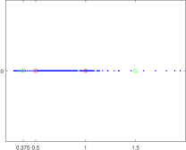
(a) $\alpha$=5.0e-1$>\nu\approx$7.22e-2

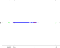
(b) $\alpha=\nu\approx$7.22e-2

(c) $\alpha$=5.0e-3$<\nu\approx$7.22e-2

(d) $\alpha$=5.0e-4$<\nu\approx$7.22e-2

(e) $\alpha$=5.0e-5$<\nu\approx$7.22e-2

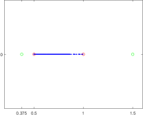
(f) $\alpha$=5.0e-6$<\nu\approx$7.22e-2

Figure 1: Spectrum of ${\bf P}_{\alpha}^{-1}{\bf K}$ corresponding to different values of $\alpha$ when $N=40$, $J=63$, $\gamma=\tau^{4}$. The blue points denotes the eigenvalues of ${\bf P}_{\alpha}^{-1}{\bf K}$. The red circles denote the two points $x=0.5$ and $x=1$. The green circles denote the two points $x=3/8$ and $x=3/2$.

From Figure 1(a), we see that the spectrum of ${\bf P}_{\alpha}^{-1}{\bf K}$ may lie outside the interval $[3/8,3/2]$ when $\alpha>\nu$. That means the setting $\alpha\in(0,\nu]$ proposed in Theorem 7 makes sense. Figures 1(a)-(b) illustrate that introducing the block $\alpha$-circulant approximations to the classical MSC preconditioner leads to perturbations in eigenvalues so that the spectrum of the preconditioned matrix is no longer completely contained in $[1/2,1]$ as the classical MSC preconditioner behaves. Figures 1 (b)-(f) demonstrates that $\sigma({\bf P}_{\alpha}^{-1}{\bf K})$ indeed lies in [3/8,3/2] for $\alpha\in(0,\nu]$, which supports the result of Theorem 7. Figures 1 (c)-(f) shows that $\sigma({\bf P}_{\alpha}^{-1}{\bf K})$ is almost contained in [1/2,1] as $\sigma({\bf P}^{-1}{\bf K})$ distributes. This is not surprising, since $\lim\limits_{\alpha\rightarrow 0^{+}}{\bf P}_{\alpha}^{-1}{\bf K}={\bf P}^{-1}{\bf K}$. On the other hand, Figures 1 (c)-(f) also indicate that [3/8,3/2] is a loose interval covering $\sigma({\bf P}_{\alpha}^{-1}{\bf K})$. The reason why we choose a loose interval has been explained in Remark 1, which is only for a simple bound $\nu$ for $\alpha$ and a tidy convergence rate of the PCG solver shown in Theorem 7.

Example 2

In this example, we consider the minimization problem (1.1) with

$$a(x_{1},x_{2})\equiv 1,\quad\Omega=(0,1)^{2},\quad T=1,\quad f(x_{1},x_{2},t)=(2\pi^{2}-1)\sin(\pi x_{2})\sin(\pi x_{1})\exp(-t),$$

$$g(x_{1},x_{2},t)=\sin(\pi x_{2})\sin(\pi x_{1})\exp(-t),$$

the analytical solution of which is given by

$$y(x_{1},x_{2},t)=\sin(\pi x_{1})\sin(\pi x_{2})\exp(-t),\quad u\equiv 0.$$

The numerical results of PCG-${\bf P}_{\alpha}$ for solving Example 2 are presented in Table 1. We observe from Table 1 that (i) the iteration numbers of the two solvers in Table 1 changes slightly as $N$ or $J$ changes; (ii) the iteration numbers of the two solvers are bounded (increasing first and then decreasing) with respect to the changes of $\gamma$. The boundedness of iteration number of PCG-${\bf P}_{\alpha}$ in Table 1 with respect to $N$, $J$ and $\gamma$ supports the theoretical results in Theorem 7. Another interesting observation from Table 2 is that the iteration numbers, errors of the two solvers are roughly the same while the CPU cost of PCG-${\bf P}_{\alpha}$ is much smaller than that of PCG-${\bf P}$ especially for large $N$. This is because ${\bf P}_{\alpha}$ is a PinT preconditioner while ${\bf P}$ is not. The smaller CPU cost of PCG-${\bf P}_{\alpha}$ compared with PCG-${\bf P}$ demonstrates the advantage of a PinT preconditioner.

Table 1: Performance of the PCG-${\bf P}_{\alpha}$ and PCG-${\bf P}$ on Example 2.

$\gamma$	$N$	$J$	$\alpha$	PCG-${\bf P}_{\alpha}$			PCG-${\bf P}$
				Iter	CPU(s)	${\rm E}_{N,J}$	Iter	CPU(s)	${\rm E}_{N,J}$
1e-7	200	961	2.85e-3	4	0.66	4.43e-3	4	4.04	4.43e-3
		3969		4	3.06	4.43e-3	4	12.36	4.43e-3
		16129		4	11.62	4.43e-3	4	42.77	4.44e-3
	400	961	7.13e-4	4	1.36	1.99e-3	4	12.20	1.99e-3
		3969		4	5.66	1.99e-3	4	41.32	1.99e-3
		16129		4	23.38	1.99e-3	4	137.84	1.99e-3
	800	961	1.78e-4	4	2.79	8.29e-4	4	37.75	8.29e-4
		3969		4	11.35	8.29e-4	4	142.26	8.29e-4
		16129		4	46.81	8.29e-4	4	446.34	8.29e-4
1e-5	200	961	2.85e-4	6	0.90	2.45e-3	6	5.17	2.4e-3
		3969		6	3.77	2.45e-3	6	15.46	2.45e-3
		16129		6	15.70	2.45e-3	6	53.49	2.45e-3
	400	961	7.13e-5	7	1.98	1.22e-3	6	15.53	1.22e-3
		3969		7	8.81	1.22e-3	6	50.17	1.22e-3
		16129		7	35.41	1.22e-3	6	179.41	1.22e-3
	800	961	1.78e-5	7	4.27	6.06e-4	6	50.26	6.06e-4
		3969		7	17.58	6.09e-4	6	172.62	6.09e-4
		16129		7	72.43	6.09e-4	6	649.47	6.09e-4
1e-3	200	961	2.85e-5	11	1.49	1.38e-3	11	9.17	1.38e-3
		3969		11	6.41	1.53e-3	11	26.04	1.53e-3
		16129		11	26.94	1.57e-3	11	95.74	1.57e-3
	400	961	7.13e-6	12	3.18	5.85e-4	10	23.97	5.85e-4
		3969		11	13.17	7.41e-4	11	90.67	7.41e-4
		16129		11	52.87	7.80e-4	11	325.89	7.80e-4
	800	961	1.78e-6	12	6.75	1.88e-4	10	75.18	1.88e-4
		3969		11	26.09	3.44e-4	11	315.21	3.44e-4
		16129		11	107.39	3.83e-4	11	1182.51	3.83e-4
1e-1	200	961	2.85e-6	7	1.01	6.16e-4	7	5.90	6.16e-4
		3969		7	4.28	1.24e-4	7	16.91	1.24e-4
		16129		7	17.92	1.20e-4	7	61.84	1.20e-4
	400	961	7.13e-7	8	2.24	6.43e-4	7	16.89	6.43e-4
		3969		7	8.72	1.41e-4	7	58.28	1.41e-4
		16129		7	35.57	6.07e-5	7	208.84	6.07e-5
	800	961	1.78e-7	8	4.73	6.57e-4	7	52.66	6.57e-4
		3969		7	17.40	1.54e-4	7	201.13	1.54e-4
		16129		7	72.01	3.10e-5	7	756.85	3.10e-5
1e1	200	961	2.85e-7	4	0.66	6.82e-4	4	3.44	6.82e-4
		3969		4	2.70	1.68e-4	4	10.16	1.68e-4
		16129		4	11.18	1.22e-4	4	36.49	1.22e-4
	400	961	7.13e-8	4	1.33	6.84e-4	4	9.87	6.84e-4
		3969		4	5.50	1.70e-4	4	33.78	1.70e-4
		16129		4	22.33	6.15e-5	4	122.00	6.15e-5
	800	961	1.78e-8	4	3.66	6.85e-4	4	30.62	6.85e-4
		3969		4	11.10	1.71e-4	4	116.08	1.71e-4
		16129		4	45.33	4.25e-5	4	436.58	4.25e-5

4.1 The Application of ${\bf P}_{\alpha}$ to A Locally Controlled Optimal Control Problem

In this subsection, we apply the proposed PinT preconditioner ${\bf P}_{\alpha}$ to the Schur complement system arising from a locally controlled optimal control problem, and present the related numerical results. The locally controlled optimal control problem is defined as follows

$$\min\limits_{y,u}L(y,u):=\frac{1}{2}||y-g||_{L^{2}(\Omega\times(0,T))}^{2}+\frac{\gamma}{2}||u||_{L^{2}(\Omega_{0}\times(0,T))}^{2},$$ (4.1)

subject to a linear wave equation with initial- and boundary-value conditions

$$\begin{cases}y_{t}-Ly=f+\chi_{\Omega_{0}}u,\quad{\rm in~{}~{}}\Omega\times(0,T),\\ y=0,\quad{\rm on~{}~{}}\partial\Omega\times(0,T),\\ y(\cdot,0)=y_{0},\quad\Omega.\end{cases}$$

The difference between the optimal control problem (1.1) and the locally controlled one (4.1) is that the regularization term $\frac{\gamma}{2}||u||_{L^{2}(\Omega_{0}\times(0,T))}^{2}$ is imposed on a subdomain $\Omega_{0}$ with $\Omega_{0}\subset\Omega$ and ${\rm Vol}(\Omega_{0})>0$. Moreover, the control variable in PDE constraint of (4.1) is weighted by the characteristic function $\chi_{\Omega_{0}}$. Here, $\chi_{\Omega_{0}}$ denotes the characteristic function of $\Omega_{0}$, which is defined as follows

$$\chi_{\Omega_{0}}(x):=\begin{cases}1,\quad x\in\Omega_{0},\\ 0,\quad{\rm otherwise}.\end{cases}$$

Similar to the discussion in Section 1 for (1.1), we can derive a reduced KKT system for (4.1) as follows

$$\left[\begin{array}[c]{cc}I&L_{2}\\ L_{1}&-\gamma^{-1}\chi_{\Omega_{0}}\end{array}\right]\left[\begin{array}[c]{c}y\\ p\end{array}\right]=\left[\begin{array}[c]{c}g\\ f\end{array}\right].$$ (4.2)

Applying the same discretization scheme as that used for approximating (1.2), we obtain the following discrete KKT system for (4.2)

$$\left[\begin{array}[c]{cc}\frac{\tau}{2}B_{2}\otimes I_{J}&B_{1}^{T}\otimes I_{J}+\frac{\tau}{2}B_{2}^{T}\otimes L_{h}\\ B_{1}\otimes I_{J}+\frac{\tau}{2}B_{2}\otimes L_{h}&-\frac{\tau}{2\gamma}B_{2}^{\rm T}\otimes I_{\Omega_{0}}\end{array}\right]\left[\begin{array}[c]{c}y_{\tau,h}\\ p_{\tau,h}\end{array}\right]=\left[\begin{array}[c]{c}g_{\tau,h}\\ f_{\tau,h}\end{array}\right].$$ (4.3)

Except for $I_{\Omega_{0}}$, other notations appearing in (4.3) are already defined in (1.3). Here, $I_{\Omega_{0}}$ is a diagonal matrix whose $i$th diagonal element is defined as follows

$$I_{\Omega_{0}}(i,i):=\begin{cases}1,\quad{\rm if~{}}i{\rm th~{}spatial~{}grid~{}point~{}locates~{}in~{}}\Omega_{0},\\ 0,\quad{\rm if~{}}i{\rm th~{}spatial~{}grid~{}point~{}locates~{}in~{}}\Omega\setminus\Omega_{0}.\end{cases}$$

Applying the same block-diagonal scaling technique used in (1.11) to (4.3), we find that solving the linear system (4.3) reduces to solving the following Schur complement system

$$(\tau I_{N}\otimes I_{\Omega_{0}}+\eta GG^{\rm T})\tilde{v}=\tilde{b},$$ (4.4)

for some given vector $\tilde{b}\in\mathbb{R}^{NJ\times 1}$. Clearly, (4.4) is a real symmetric positive definite system, as $G$ (see the definition in (2.12)) is non-singular. Hence, both PCG-${\bf P}_{\alpha}$ and PCG-${\bf P}$ are applicable to solving (4.4).

Example 3

In this example, we consider the locally controlled optimal control problem (4.1) with

$$a(x_{1},x_{2})\equiv 1,\quad\Omega=(0,1)^{2},\quad T=1,\quad f(x_{1},x_{2},t)=(2\pi^{2}-1)\sin(\pi x_{2})\sin(\pi x_{1})\exp(-t),$$

$$g(x_{1},x_{2},t)=\sin(\pi x_{2})\sin(\pi x_{1})\exp(-t),\quad\Omega_{0}:=(0,1)^{2}\setminus(0,0.5)^{2},$$

the analytical solution of which is given by

$$y(x_{1},x_{2},t)=\sin(\pi x_{1})\sin(\pi x_{2})\exp(-t),\quad u\equiv 0.$$

We apply PCG-${\bf P}_{\alpha}$ and PCG-${\bf P}$ to solving Example 3, the numerical results of which are presented in Table 3. From Table 3, we see that the CPU cost pf PCG-${\bf P}_{\alpha}$ is much smaller than that of PCG-${\bf P}$ while the iteration numbers and errors of the two solvers are roughly the same. This again demonstrates the superiority of the proposed PinT preconditioner over the non-PinT preconditioner ${\bf P}$ in terms of computational time. Another observation from Table 2 is that the iteration number of the both solvers decreases as $\gamma$ increases. The reason may be explained as follows. Both ${\bf P}_{\alpha}$ and ${\bf P}$ are originally designed for approximating the matrix $(\tau I_{N}\otimes I_{J}+\eta GG^{\rm T})$ while in Example 3, ${\bf P}_{\alpha}$ and ${\bf P}$ are used as preconditioners of $(\tau I_{N}\otimes I_{\Omega_{0}}+\eta GG^{\rm T})$. Recall that $\eta=\gamma/\tau$. When $\gamma$ increases, $\eta GG^{\rm T}$ becomes dominant and $(\tau I_{N}\otimes I_{\Omega_{0}}+\eta GG^{\rm T})$ behaves more like $(\tau I_{N}\otimes I_{x}+\eta GG^{\rm T})$ in spectral sense. Therefore, when $\gamma$ is not small, ${\bf P}_{\alpha}$ and ${\bf P}$ approximate $(\tau I_{N}\otimes I_{\Omega_{0}}+\eta GG^{\rm T})$ well in spectral sense and both solvers converges quickly in such case. Hence, ${\bf P}_{\alpha}$ is an efficient preconditioner for locally controlled optimal control problem when $\gamma$ is not small.

Table 2: Performance of the PCG-${\bf P}_{\alpha}$ and PCG-${\bf P}$ on Example 3.

$\gamma$	$N$	$J$	$\alpha$	PCG-${\bf P}_{\alpha}$			PCG-${\bf P}$
				Iter	CPU(s)	${\rm E}_{N,J}$	Iter	CPU(s)	${\rm E}_{N,J}$
1e-4	100	961	3.61e-4	24	1.60	4.61e-3	23	8.44	4.61e-3
		3969		23	7.15	4.63e-3	23	20.32	4.63e-3
		16129		23	29.50	4.63e-3	23	64.71	4.63e-3
	200	961	9.02e-5	25	3.59	2.29e-3	23	20.11	2.29e-3
		3969		24	15.23	2.30e-3	23	59.25	2.30e-3
		16129		24	60.85	2.31e-3	23	206.51	2.31e-3
	400	961	2.26e-5	25	7.54	1.14e-3	23	62.20	1.14e-3
		3969		25	31.23	1.15e-3	23	199.52	1.15e-3
		16129		25	128.73	1.15e-3	23	716.28	1.15e-3
1e-3	100	961	1.14e-4	15	1.14	2.72e-3	14	4.78	2.72e-3
		3969		15	4.77	2.90e-3	14	12.06	2.90e-3
		16129		15	19.87	2.95e-3	14	39.27	2.95e-3
	200	961	2.85e-5	15	2.24	1.25e-3	14	12.22	1.24e-3
		3969		15	9.75	1.42e-3	14	36.04	1.42e-3
		16129		15	39.32	1.47e-3	14	124.66	1.47e-3
	400	961	7.13e-6	15	4.66	5.23e-4	14	39.80	5.23e-4
		3969		15	19.60	6.83e-4	14	127.06	6.83e-4
		16129		15	79.89	7.27e-4	14	426.76	7.27e-4
1e-2	100	961	3.61e-5	11	0.77	2.40e-4	11	3.75	2.40e-4
		3969		11	3.60	5.59e-4	11	9.50	5.59e-4
		16129		11	15.00	6.68e-4	11	30.80	6.68e-4
	200	961	9.02e-6	11	1.65	3.35e-4	11	9.59	3.35e-4
		3969		11	7.38	2.09e-4	11	28.26	2.09e-4
		16129		11	29.84	3.14e-4	11	96.93	3.14e-4
	400	961	2.26e-6	11	3.47	4.54e-4	11	28.83	4.54e-4
		3969		11	14.69	5.98e-5	11	91.70	5.98e-5
		16129		11	59.93	1.39e-4	11	330.21	1.39e-4
1e-1	100	961	1.14e-5	7	0.59	5.93e-4	8	2.76	5.93e-4
		3969		7	2.35	2.43e-4	8	6.91	2.43e-4
		16129		7	9.99	2.40e-4	8	22.93	2.40e-4
	200	961	2.85e-6	7	1.11	6.36e-4	8	6.82	6.36e-4
		3969		7	4.88	1.30e-4	8	20.69	1.30e-4
		16129		7	19.80	1.21e-4	8	71.53	1.21e-4
	400	961	7.13e-7	8	2.61	6.56e-4	7	18.27	6.56e-4
		3969		7	9.93	1.50e-4	8	67.01	1.50e-4
		16129		7	43.19	6.09e-5	8	241.76	6.09e-5
1	100	961	3.61e-6	5	0.44	6.67e-4	6	2.11	6.67e-4
		3969		5	1.78	2.45e-4	6	5.34	2.45e-4
		16129		5	7.47	2.42e-4	6	17.53	2.42e-4
	200	961	9.02e-7	5	0.84	6.78e-4	6	5.27	6.78e-4
		3969		5	3.66	1.65e-4	6	15.63	1.65e-4
		16129		5	14.88	1.22e-4	6	54.30	1.22e-4
	400	961	2.26e-7	5	1.78	6.82e-4	5	13.38	6.82e-4
		3969		5	7.34	1.68e-4	6	50.78	1.68e-4
		16129		5	30.16	6.14e-5	6	182.79	6.14e-5

5 Concluding Remarks

In this paper, a PinT preconditioner has been proposed for the Schur complement system arising from the parabolic PDE-constrained optimal control problem. Theoretically, we have shown that the spectrum of the preconditioned matrix is lower and upper bounded by positive constants independent of matrix size and the regularization parameter, thanks to which PCG solver for the preconditioned system has been proven to have an optimal convergence rate. Numerical results reported have shown the efficiency of the proposed preconditioning technique and supported the theoretical results.

References

• Abbeloos et al. [2011] Dirk Abbeloos, Moritz Diehl, Michael Hinze, and Stefan Vandewalle. Nested multigrid methods for time-periodic, parabolic optimal control problems. Computing and visualization in science, 14(1):27, 2011.
• Apel and Flaig [2012] Thomas Apel and Thomas G Flaig. Crank–Nicolson schemes for optimal control problems with evolution equations. SIAM Journal on Numerical Analysis, 50(3):1484–1512, 2012.
• Axelsson and Lindskog [1986] Owe Axelsson and Gunhild Lindskog. On the rate of convergence of the preconditioned conjugate gradient method. Numerische Mathematik, 48(5):499–523, 1986.
• Axelsson and Neytcheva [2003] Owe Axelsson and Maya Neytcheva. Preconditioning methods for linear systems arising in constrained optimization problems. Numerical linear algebra with applications, 10(1-2):3–31, 2003.
• Benzi et al. [2005] Michele Benzi, Gene H Golub, and Jörg Liesen. Numerical solution of saddle point problems. Acta Numer., 14:1–137, 2005.
• Biegler et al. [2007] Lorenz T Biegler, Omar Ghattas, Matthias Heinkenschloss, David Keyes, and Bart van Bloemen Waanders. Real-time PDE-constrained Optimization. SIAM, 2007.
• Bini et al. [2005] D. Bini, G. Latouche, and B. Meini. Numerical Methods for Structured Markov Chains. Oxford University Press: New York, 2005.
• Cao et al. [2016] Yang Cao, Zhi-Ru Ren, and Quan Shi. A simplified HSS preconditioner for generalized saddle point problems. BIT Numerical Mathematics, 56:423–439, 2016.
• de Sturler and Liesen [2005] Eric de Sturler and Jörg Liesen. Block-diagonal and constraint preconditioners for nonsymmetric indefinite linear systems. part i: Theory. SIAM Journal on Scientific Computing, 26(5):1598–1619, 2005.
• Donald [2016] E Donald. Optimal control theory: an introduction. DOVER PUBNS, 2016.
• Elman et al. [2014] H. C. Elman, D. J. Silvester, and A. J. Wathen. Finite elements and fast iterative solvers: with applications in incompressible fluid dynamics. Numerical Mathematics and Scie, 2014.
• Falgout et al. [2014] Robert D Falgout, Stephanie Friedhoff, Tz V Kolev, Scott P MacLachlan, and Jacob B Schroder. Parallel time integration with multigrid. SIAM J. Sci. Comput., 36(6):C635–C661, 2014.
• Franceschini et al. [2019] Andrea Franceschini, Nicola Castelletto, and Massimiliano Ferronato. Block preconditioning for fault/fracture mechanics saddle-point problems. Computer Methods in Applied Mechanics and Engineering, 344:376–401, 2019.
• Gander [2015] Martin J Gander. 50 years of time parallel time integration. In Multiple Shooting and Time Domain Decomposition Methods, pages 69–113. Springer, 2015.
• Gander and Neumuller [2016] Martin J Gander and Martin Neumuller. Analysis of a new space-time parallel multigrid algorithm for parabolic problems. SIAM J. Sci. Comput., 38(4):A2173–A2208, 2016.
• Gander and Palitta [2023] Martin J Gander and Davide Palitta. A new paradiag time-parallel time integration method. arXiv preprint arXiv:2304.12597, 2023.
• Gander and Vandewalle [2007] Martin J Gander and Stefan Vandewalle. Analysis of the parareal time-parallel time-integration method. SIAM J. Sci. Comput., 29(2):556–578, 2007.
• Gander and Wu [2019] Martin J Gander and Shu-Lin Wu. Convergence analysis of a periodic-like waveform relaxation method for initial-value problems via the diagonalization technique. Numer. Math., 143(2):489–527, 2019.
• Gander et al. [2016] Martin J Gander, Laurence Halpern, Juliet Ryan, and Thuy Thi Bich Tran. A direct solver for time parallelization. In Domain Decomposition Methods in Science and Engineering XXII, pages 491–499. Springer, 2016.
• Gander et al. [2020] Martin J Gander, Jun Liu, Shu-Lin Wu, Xiaoqiang Yue, and Tao Zhou. Paradiag: Parallel-in-time algorithms based on the diagonalization technique. arXiv preprint arXiv:2005.09158, 2020.
• Gu and Wu [2020] Xian-Ming Gu and Shu-Lin Wu. A parallel-in-time iterative algorithm for volterra partial integro-differential problems with weakly singular kernel. Journal of Computational Physics, 417:109576, 2020.
• Hackbusch [1985] Wolfgang Hackbusch. Parabolic multi-grid methods. In Proc. of the sixth int’l. symposium on Computing methods in applied sciences and engineering, VI, pages 189–197. North-Holland Publishing Co., 1985.
• Hon [2022] Sean Hon. Optimal block circulant preconditioners for block Toeplitz systems with application to evolutionary PDEs. Journal of Computational and Applied Mathematics, 407:113965, 2022.
• Hon and Serra-Capizzano [2022] Sean Hon and Stefano Serra-Capizzano. A sine transform based preconditioned minres method for all-at-once systems from evolutionary partial differential equations. arXiv preprint arXiv:2201.10062, 2022.
• Horton and Vandewalle [1995] Graham Horton and Stefan Vandewalle. A space-time multigrid method for parabolic partial differential equations. SIAM J. Sci. Comput., 16(4):848–864, 1995.
• Ipsen [2001] Ilse CF Ipsen. A note on preconditioning nonsymmetric matrices. SIAM Journal on Scientific Computing, 23(3):1050–1051, 2001.
• Kunisch and Rund [2015] Karl Kunisch and Armin Rund. Time optimal control of the monodomain model in cardiac electrophysiology. IMA J. Appl. Math., 80(6):1664–1683, 2015.
• Kwok and Ong [2019] Felix Kwok and Benjamin W Ong. Schwarz waveform relaxation with adaptive pipelining. SIAM J. Sci. Comput., 41(1):A339–A364, 2019.
• Leitmann [1981] George Leitmann. The calculus of variations and optimal control, volume 24. Springer Science & Business Media, 1981.
• Lin and Ng [2021] Xue-Lei Lin and M. K. Ng. An all-at-once preconditioner for evolutionary partial differential equations. SIAM J. Sci. Comput., 43(4):A2766–A2784, 2021.
• Lin et al. [2021] Xue-lei Lin, Michael K Ng, and Yajing Zhi. A parallel-in-time two-sided preconditioning for all-at-once system from a non-local evolutionary equation with weakly singular kernel. Journal of Computational Physics, 434:110221, 2021.
• Lin et al. [2018] Xuelei Lin, Michael K Ng, and Haiwei Sun. A separable preconditioner for time-space fractional caputo-riesz diffusion equations. Numer. Math. Theor. Meth. Appl, 11:827–853, 2018.
• Lions et al. [2001] Jacques-Louis Lions, Yvon Maday, and Gabriel Turinici. A parareal in time discretization of PDEs. C.R.Acad. Sci. Paris, Serie I, 332(7):661 – 668, 2001. doi: https://doi.org/10.1016/S0764-4442(00)01793-6.
• Liu and Pearson [2020] Jun Liu and John W Pearson. Parameter-robust preconditioning for the optimal control of the wave equation. Numerical Algorithms, 83(3):1171–1203, 2020.
• Liu and Wang [2022] Jun Liu and Zhu Wang. A ROM-accelerated parallel-in-time preconditioner for solving all-at-once systems in unsteady convection-diffusion PDEs. Applied Mathematics and Computation, 416:126750, 2022.
• Liu and Wu [2020] Jun Liu and Shu-Lin Wu. A fast block $\alpha$-circulant preconditoner for all-at-once systems from wave equations. SIAM Journal on Matrix Analysis and Applications, 41(4):1912–1943, 2020.
• Liu et al. [2022] Jun Liu, Xiang-Sheng Wang, Shu-Lin Wu, and Tao Zhou. A well-conditioned direct PinT algorithm for first-and second-order evolutionary equations. Advances in Computational Mathematics, 48(3):16, 2022.
• Loghin and Wathen [2004] Daniel Loghin and Andrew J Wathen. Analysis of preconditioners for saddle-point problems. SIAM Journal on Scientific Computing, 25(6):2029–2049, 2004.
• McDonald et al. [2018] E. McDonald, J. Pestana, and A. Wathen. Preconditioning and iterative solution of all-at-once systems for evolutionary partial differential equations. SIAM J. Sci. Comput., 40(2):A1012–A1033, 2018.
• McDonald et al. [2017] Eleanor McDonald, Sean Hon, Jennifer Pestana, and Andy Wathen. Preconditioning for nonsymmetry and time-dependence. In Domain Decomposition Methods in Science and Engineering XXIII, pages 81–91. Springer, 2017.
• Miele [1975] Angelo Miele. Recent advances in gradient algorithms for optimal control problems. Journal of Optimization Theory and Applications, 17:361–430, 1975.
• Murphy et al. [2000] Malcolm F Murphy, Gene H Golub, and Andrew J Wathen. A note on preconditioning for indefinite linear systems. SIAM Journal on Scientific Computing, 21(6):1969–1972, 2000.
• Ng [2004] M. K. Ng. Iterative methods for Toeplitz systems. Numerical Mathematics and Scie, 2004.
• Notay [2014] Yvan Notay. A new analysis of block preconditioners for saddle point problems. SIAM journal on Matrix Analysis and Applications, 35(1):143–173, 2014.
• Pearson and Wathen [2012] John W Pearson and Andrew J Wathen. A new approximation of the Schur complement in preconditioners for PDE-constrained optimization. Numerical Linear Algebra with Applications, 19(5):816–829, 2012.
• Pearson et al. [2012] John W Pearson, Martin Stoll, and Andrew J Wathen. Regularization-robust preconditioners for time-dependent PDE-constrained optimization problems. SIAM J. Matrix Anal. Appl., 33(4):1126–1152, 2012.
• Polak [1973] Elijah Polak. An historical survey of computational methods in optimal control. SIAM review, 15(2):553–584, 1973.
• Quirynen and Di Cairano [2020] Rien Quirynen and Stefano Di Cairano. Presas: Block-structured preconditioning of iterative solvers within a primal active-set method for fast model predictive control. Optimal Control Applications and Methods, 41(6):2282–2307, 2020.
• Rao [2009] Anil V Rao. A survey of numerical methods for optimal control. Advances in the Astronautical Sciences, 135(1):497–528, 2009.
• Rees [2010] Tyrone Rees. Preconditioning iterative methods for PDE constrained optimization. PhD thesis, University of Oxford Oxford, UK, 2010.
• Sogn and Zulehner [2019] Jarle Sogn and Walter Zulehner. Schur complement preconditioners for multiple saddle point problems of block tridiagonal form with application to optimization problems. IMA Journal of Numerical Analysis, 39(3):1328–1359, 2019.
• Tröltzsch [2010] Fredi Tröltzsch. Optimal control of partial differential equations: theory, methods, and applications, volume 112. American Mathematical Soc., 2010.
• Vandewalle [2013] Stefan Vandewalle. Parallel multigrid waveform relaxation for parabolic problems. Springer-Verlag, 2013.
• Von Stryk and Bulirsch [1992] Oskar Von Stryk and Roland Bulirsch. Direct and indirect methods for trajectory optimization. Annals of operations research, 37:357–373, 1992.
• Wang et al. [2004] Yao-Wen Wang, Wen-Jian Cai, Yeng-Chai Soh, Shu-Jiang Li, Lu Lu, and Lihua Xie. A simplified modeling of cooling coils for control and optimization of hvac systems. Energy Conversion and Management, 45(18-19):2915–2930, 2004.
• Wang [2009] Zeng-Qi Wang. Optimization of the parameterized uzawa preconditioners for saddle point matrices. Journal of computational and applied mathematics, 226(1):136–154, 2009.
• Wathen and Goddard [2019] A Wathen and A Goddard. A note on parallel preconditioning for all-at-once evolutionary PDEs. Electron. Trans. Numer. Anal., 2019.
• Wathen et al. [1995] Andrew Wathen, Bernd Fischer, and David Silvester. The convergence rate of the minimal residual method for the stokes problem. Numer. Math., 71:121–134, 1995.
• Wu [2018] Shu-Lin Wu. Toward parallel coarse grid correction for the parareal algorithm. SIAM J. Sci. Comput., 40(3):A1446–A1472, 2018.
• Wu and Liu [2020] Shu-Lin Wu and Jun Liu. A parallel-in-time block-circulant preconditioner for optimal control of wave equations. SIAM Journal on Scientific Computing, 42(3):A1510–A1540, 2020.
• Wu and Zhou [2019] Shu-Lin Wu and Tao Zhou. Acceleration of the two-level MGRIT algorithm via the diagonalization technique. SIAM J. Sci. Comput., 41(5):A3421–A3448, 2019.
• Wu and Zhou [2020] Shu-Lin Wu and Tao Zhou. Diagonalization-based parallel-in-time algorithms for parabolic PDE-constrained optimization problems. ESAIM: Control, Optimisation and Calculus of Variations, 26:88, 2020.