Macroscopic delayed-choice and retrocausality: quantum eraser, Leggett-Garg and dimension witness tests with cat states

Abstract

We propose delayed choice experiments carried out with macroscopic qubits, realised as macroscopically-distinct coherent states $|\alpha\rangle$ and $|-\alpha\rangle$. Quantum superpositions of $|\alpha\rangle$ and $|-\alpha\rangle$ are created via a unitary interaction $U(\theta)$ based on a nonlinear Hamiltonian, in analogy with polarising beam splitters used in photonic experiments. Macroscopic delayed-choice experiments give a compelling reason to develop interpretations not allowing macroscopic retrocausality (MrC). We therefore consider weak macroscopic realism (wMR), which specifies a hidden variable $\lambda_{\theta}$ to determine the macroscopic qubit value (analogous to ’which-way’ information), independent of any future measurement setting $\phi$. Using entangled cat states, we demonstrate a quantum eraser where the choice to measure a which-way or wave-type property is delayed. Consistency with wMR is possible, if we interpret the macroscopic qubit value to be determined by $\lambda_{\theta}$ without specification of the state at the level of order $\hbar$, where fringes manifest. We then demonstrate violations of a delayed-choice Leggett-Garg inequality, and of the dimension witness inequality applied to the Wheeler-Chaves-Lemos-Pienaar experiment, where measurements need only distinguish the macroscopic qubit states. This negates all two-dimensional non-retrocausal models, thereby suggesting MrC. However, one can interpret consistently with wMR, thus avoiding conclusions of MrC, by noting extra dimensions, and by noting that the violations require further unitary dynamics $U$ for each system. The violations are then explained as failure of deterministic macroscopic realism (dMR), which specifies validity of $\lambda_{\theta}$ prior to the dynamics $U(\theta)$ determining the measurement setting $\theta$. Finally, although there is consistency with wMR for macroscopic observations, we demonstrate Einstein-Podolsky-Rosen-type paradoxes at a microscopic level, based on fringe distributions.

I Introduction

Gedanken experiments in which there is a delayed choice of measurement motivated Wheeler and others to consider whether quantum mechanics implied a failure of realism, or else retrocausality wheeler-retro ; wheeler-retro-2 ; ma-zeilinger-rmp-delay-choice . The central argument has been presented for the two-slit experiment, in which a photon travels through the slits exhibiting either particle or wave-like behaviour. The observation of an interference pattern is interpreted as wave-like behaviour, while the observation that the photon travelled along a single path is interpreted as particle-like behaviour. A similar proposal exists for a Mach-Zehnder (MZ) interferometer, in which the photon travels in one or other path associated with the outputs of a beam splitter wheeler-retro ; wheeler-retro-2 . In the delayed-choice quantum eraser delayed-choice-qubit-scully-druhl , the decision to observe either the wave or particle-like behaviour is delayed until after the photon has passed through the apparatus, and the fringe distribution vanishes or emerges, conditionally on the measurement made at the later time. Thus there is an apparently paradoxical situation whereby it seems as though whether the photon went through “both slits” or “one slit” can be changed by an event (the choice of measurement) in the future.

Multiple different refinements and interpretations have been given scully-englert-walther ; kim-scully-entangled-quantum-eraser-experiment ; walborn-double-slit-quantum-eraser-experiment ; herzog-zeilinger-quantum-eraser-complementarity-exp ; jacques-aspect-experiment-wheeler ; truscott-atoms-delayed-choice ; tang-exp-wheeler-delayed-choice ; Ma-zeilinger-exp-causal-delayed-choice-interpretation ; englert-scully-walther-double-slit-am-journ-phy ; mohrhoff-delayed-choice-interpret-am-journ-phy ; ingraham-nonlocality-delay-choice ; ma-zeilinger-rmp-delay-choice ; kastner-quantum-eraser-interpret-found-phy ; la-cour-yudichak-classical-quantum-eraser-dim-wit ; Ionicioiu-terno ; IT-ent1 ; IT-ent-2 ; ITent3 ; quantum-bs-I-terno-experiment ; kaiser-coudreau-milman-experiment-ent-delayed-choice ; zheng-quantum-delayed-choiceBS-exp ; delayed-choice-causal-model-chaves ; delayed-choice-experiment-chaves ; huang-delayed-choice-causal-model-compatibility ; faetti-quantum-eraser-ent-interpretation-1 , but the consensus is that the original delayed-choice experiments do not imply the need for retrocausality. The above paradox arises only if one views the system as being either a wave or particle. The work of Ionicioiu and Terno proposed a quantum beam splitter Ionicioiu-terno , which would place the system in a quantum superposition of wave- and particle-like states. An intermediate regime can be quantified, and a class of hidden variable theories based on the assumption of either wave- or particle-like behaviour can be negated Ionicioiu-terno ; IT-ent1 . Significantly, Chaves, Lemos and Pienaar (CLP) resolved these issues further by explicitly constructing a two-dimensional causal model to explain the original MZ delayed-choice experiment delayed-choice-causal-model-chaves , thus ruling out any need for retrocausal explanations.

On the other hand, with the inclusion of an additional phase shift in the MZ interferometer, CLP demonstrated that a two-dimensional classical model would need to be retrocausal to explain the predicted observations, which lead to a violation of a dimension witness inequality. Recent experiments confirm these predictions delayed-choice-experiment-chaves ; huang-delayed-choice-causal-model-compatibility . In their analysis, the meaning of “non-retrocausal” is that, in a model which assumes realism, hidden variables $\lambda$ associated with the preparation state are independent of any future measurement setting, $\phi$. La Cour and Yudichak recently give a model which is nonretrocausal, but possesses extra dimensions la-cour-yudichak-classical-quantum-eraser-dim-wit . Their model however is based on stochastic electrodynamics, which is not equivalent to quantum mechanics.

In this paper, we propose and analyse macroscopic versions of delayed-choice experiments. Our results demonstrate that delayed-choice paradoxes and the causal-modelling tests of CLP are evident at a macroscopic level, beyond $\hbar$, without the need for a microscopic resolution of measurement outcomes. Since retrocausality is more paradoxical at a macroscopic level, we argue that this strengthens the need to explain the results of the experiments without invoking retrocausality.

Specifically, we follow manushan-cat-lg ; manushan-bell-cat-lg ; macro-bell-lg and map from a microscopic to a macroscopic regime, where spin qubits $|\uparrow\rangle$ and $|\downarrow\rangle$ are realised as macroscopically distinct coherent states $|\alpha\rangle$ and $|-\alpha\rangle$ ($\alpha$ is large), that form a macroscopic qubit. The qubit values $\eta$ of $+1$ and $-1$ corresponding to the coherent states $|\alpha\rangle$ and $|-\alpha\rangle$ can be distinguished by a measurement of the field quadrature amplitude $X$, without the need to resolve at the level of $\hbar$. In analogy with a polarising beam splitter (PBS) used in the photonic experiments, superpositions of the two coherent states (called cat states) manushan-cat-lg ; manushan-bell-cat-lg ; macro-bell-lg ; yurke-stoler-1

$$\cos\theta|\alpha\rangle+i\sin\theta|-\alpha\rangle$$ (1)

can be created using a unitary interaction $U(t)\equiv U(\theta)$ based on a nonlinear Hamiltonian, $H_{NL}$. The value of $t$ determines $\theta$ and hence the probability amplitudes of the two-state superposition. This provides a mechanism for a direct mapping from the microscopic to macroscopic delayed-choice experiments.

To analyse quantitatively, we seek to define macroscopic retrocausality. In analyses of the delayed-choice experiments, the meaning of retrocausality is intertwined with that of realism. Our approach is therefore closely linked to that of Leggett and Garg legggarg-1 and indeed we propose a delayed-choice version of the Leggett-Garg violation of macro-realism, showing violation of Leggett-Garg inequalities uisng cat states. Following Leggett and Garg, we define macroscopic realism: Macroscopic realism asserts a predetermination of the outcome for a measurement of the macroscopic qubit value $\eta$ (the sign of $X$), for the system prepared at time $t_{M}$ in a superposition (1). The variable $\lambda_{M}$ describes the macroscopic state of the system at the time $t_{M}$ and its value gives the outcome of the qubit measurement $\eta$. Since the value does not require a microscopic resolution, the validity of $\lambda_{M}$ at the given time $t_{M}$ is a very weak assumption, compared to the assumption of Bell’s local hidden-variable states $\{\lambda_{i}\}$ bell-3 which give a realistic description for any measurement, including those that are microscopically resolved. The cat-state analysis enables a clear distinction between the macroscopic hidden variable $\lambda_{M}$ and the more general hidden-variable states $\{\lambda_{i}\}$.

However, recent work establishes the need to also carefully consider whether the unitary rotation $U(\theta)$ associated with the measurement setting $\theta$ has been performed (or not) prior to $t_{M}$. This leads to two definitions of macroscopic realism, one of which (deterministic macroscopic realism) can be falsified macro-bell-lg ; manushan-bell-cat-lg . Deterministic macroscopic realism (dMR) asserts a predetermination of outcomes, at a time $t$, for multiple future choices of $\theta$ (e.g. $\theta_{1}$ and $\theta_{2}=\phi$), so that these outcomes are given by multiple hidden variables (e.g. $\lambda_{M1}$ and $\lambda_{M2}$) simultaneously specified at $t$.

To examine macroscopic retrocausality, we therefore consider weak macroscopic realism (wMR) manushan-bell-cat-lg : Weak macroscopic realism asserts that the system prepared at time $t_{M}$ in a superposition (1) is in a state giving a definite outcome $\lambda_{M}$ ($\lambda_{M}$ being $+1$ or $-1$) for the macroscopic pointer qubit measurement $\eta$. It is implicit as part of the definition that the value $\lambda_{M}$ be independent of any future measurement setting, $\phi$. We use the term pointer measurement, because it is assumed that the unitary rotation $U(\theta)$ determining the measurement setting has already been performed, prior to $t_{M}$ i.e. the system has been prepared in the appropriate basis, $\theta$.

In this paper, we examine the unitary dynamics $U(t)$, showing that at certain times $t_{M}$ the assumption of $\lambda_{M}$ is relevant, because the system is in a two-state superposition (1). During the dynamics, however, the state of the system has a more general form than (1). Extra dimensions are evident in the quantum continuous-variable phase-space representations for the system. Thus, it is possible to argue consistently with the Chaves-Lemos-Pienaar (CLP) analysis that $\lambda_{M}$ is valid at the time $t_{M}$, and hence that there is no macroscopic retrocausality. Instead, the violations of the dimensions witness inequality and delayed-choice Leggett-Garg inequalities reflect the failure of dMR, which (it is argued) arises from failure of Bell-type hidden variables $\{\lambda_{i}\}$ defined microscopically.

In summary, the main results of this paper are two-fold: First, we demonstrate the possibility of performing macroscopic delayed-choice tests using cat states, including those of the type previously proposed at a microscopic level by CLP. Second, we explain how these predictions can be viewed consistently with wMR, thus providing a counter argument to any conclusions of macroscopic retrocausality. Lastly, although there is no inconsistency with wMR at a macroscopic level, we point out EPR-type paradoxes epr-1 ; manushan-bell-cat-lg giving inconsistencies with the completeness of quantum mechanics at a microscopic level, where fringes in the distributions are evident.

II summary of paper

The paper is organised as follows. In section III, we consider a quantum eraser experiment. In analogy with experiments using entangled states kim-scully-entangled-quantum-eraser-experiment ; kaiser-coudreau-milman-experiment-ent-delayed-choice ; ma-zeilinger-rmp-delay-choice , the system is prepared at $t_{1}=0$ in a two-mode entangled cat state $\sim|\alpha\rangle_{a}|-\beta\rangle_{b}-|-\alpha\rangle_{a}|\beta\rangle_{b}$. We identify the qubit value $\eta_{i}$ at time $t_{i}$ as “which-way” information. The qubit value for $a$ can be determined by a quadrature measurement $X_{B}$ of the mode $b$, and the interference for system $a$ created by interacting locally according to $U_{A}(t_{2})$ for a specific time $t_{2}$. Similarly, one may apply $U_{B}(t_{2})$ for $b$. The loss of which-way information is identified by fringes in the distributions of the orthogonal quadrature $P_{A}$ for $a$. However, we conclude there is no paradox involving macroscopic retrocausality, since the fringes are only distinguished at the level of $\hbar$. The results can be viewed consistently with weak macroscopic realism. Nonetheless, in Section VI we show that at the microscopic level of $\hbar$, EPR-type paradoxes can be constructed (similar to those discussed in macro-coherence-paradox ; manushan-bell-cat-lg ), based on the fringe pattern.

We turn to macroscopic paradoxes, in Section IV, by presenting tests where it is only necessary to measure the macroscopic qubit value $\eta$. We show violation of a Leggett-Garg inequality, where one measures $\eta_{i}$ at three times $t_{i}$ ($t_{3}>t_{2}>t_{1}$). The violation reveals failure of the joint assumptions of weak macroscopic realism (wMR) and noninvasive measurability (called macrorealism). Noninvasive measurability asserts that one can determine the value of $\lambda_{i}$ for the system satisfying wMR, in a way that does not affect the future $\lambda_{j}$ ($j>i$). In the present proposal, the measurement of $\lambda_{i}$ ($i=1,2$) of $a$ is justified to be noninvasive because it is performed on the spacelike separated system $b$ and, furthermore, the choice of which measurement ($\lambda_{1}$ or $\lambda_{2}$) to make is delayed, until after $t_{3}$. A natural interpretion is that the measurement of $\lambda_{2}$ (or $\lambda_{1}$) disturbs the dynamics to affect the result for $\lambda_{3}$, therefore violating macrorealism. Since there is a delayed choice, this suggests macroscopic retrocausality. In Section V, we follow the Chaves-Lemos-Pienaar experiment, demonstrating violation of the dimension witness inequality for cat states, thus falsifying all two-dimensional non-retrocausal models delayed-choice-causal-model-chaves . This consolidates the work of manushan-bell-cat-lg , which outlined the possibility of delayed-choice experiments with cat states.

To counter conclusions of macroscopic retrocausality, in Section IV.C we give an interpretation of the violations of the delayed-choice Leggett-Garg inequalities that is consistent with wMR: The apparent macroscopic retrocausality comes about because of the entanglement with the meter system $b$ at the time $t_{2}$, and the macroscopic nonlocality associated with the dynamics of the unitary rotations, when such rotations occur for both systems after the time $t_{2}$. Using phase-space depictions of $P(X_{A},X_{B})$, we identify extra dimensions not present in the two-dimensional non-retrocausal models. We show that the violation of the Leggett-Garg inequalities certifies a failure of deterministic macroscopic realism (dMR), but not wMR (which is a weaker assumption than dMR). A similar explanation is given in Section V to explain the violation of the dimension witness inequality.

III Delayed-choice quantum eraser with entangled cat states

III.1 Set-up

We begin by presenting an analogue of the delayed-choice quantum eraser experiment, for cat states. We consider the variant that uses two spatially separated systems $A$ and $B$. The overall system is prepared at time $t_{1}=0$ in the entangled cat Bell state cat-bell-wang-1

$$|\psi_{Bell}(t_{1})\rangle=\mathcal{N}\{|\alpha\rangle|-\beta\rangle-|-\alpha\rangle|\beta\rangle\}$$ (2)

where $|\alpha\rangle$ and $|\beta\rangle$ are coherent states for single-mode systems $A$ and $B$. We take $\alpha$ and $\beta$ to be real, positive and large. Here, $\mathcal{N}=\frac{1}{\sqrt{2}}\{1-\exp(-2\left|\alpha\right|^{2}-2\left|\beta\right|^{2})\}^{-1/2}$ is the normalisation constant.

For each system, one may measure the field quadrature phase amplitudes $\hat{X}_{A}={\color[rgb]{1,0,0}{\color[rgb]{0,0,1}{\color[rgb]{0,0,0}\frac{1}{\sqrt{2}}}}}(\hat{a}+\hat{a}^{\dagger})$, $\hat{P}_{A}={\color[rgb]{1,0,0}{\color[rgb]{0,0,1}{\color[rgb]{0,0,0}\frac{1}{i\sqrt{2}}}}}(\hat{a}-\hat{a}^{\dagger})$, $\hat{X}_{B}=\frac{1}{\sqrt{2}}(\hat{b}+\hat{b}^{\dagger})$ and $\hat{P}_{A}={\color[rgb]{1,0,0}{\color[rgb]{0,0,1}{\color[rgb]{0,0,0}\frac{1}{i\sqrt{2}}}}}(\hat{a}-\hat{a}^{\dagger})$, which are defined in a rotating frame, with units so that $\hbar=1$ yurke-stoler-1 . The boson destruction mode operators for modes $A$ and $B$ are denoted by $\hat{a}$ and $\hat{b}$, respectively. The outcome $X_{A}$ of the measurement $\hat{X}_{A}$ distinguishes between the states $|\alpha\rangle$ and $|-\alpha\rangle$, and similarly $\hat{X}_{B}$ distinguishes between the states $|\beta\rangle$ and $|-\beta\rangle$. We define the outcome of the measurement $\hat{S}^{(A)}$ to be $S^{(A)}=+1$ if $X_{A}>0$, and $-1$ otherwise. Similarly, the outcome of the measurement $\hat{S}^{(B)}$ is $S^{(B)}=+1$ if $X_{B}>0$, and $-1$ otherwise. $S$ is identified as the spin of the system i.e. the qubit value $\eta$.

The coherent states of $A$ and $B$ become orthogonal in the limit of large $\alpha$ and $\beta$, in which case the superposition (2) maps onto the two-qubit Bell state

$$|\psi_{Bell}\rangle=\frac{1}{\sqrt{2}}(|+\rangle_{a}|-\rangle_{b}-|-\rangle_{a}|+\rangle_{b})$$ (3)

At time $t_{1}$, the outcomes for $S^{(A)}$ and $S^{(B)}$ are anti-correlated. Therefore, one may infer the outcome for $S^{(A)}$ noninvasively by measuring $X_{B}$, and hence $S^{(B)}$.

We present an analogy with the delayed-choice quantum eraser based on the photonic versions of the state (3). In the photonic version, the next step is that the photon of system $A$ propagates through two slits, or else through a 50/50 beam splitter ($BS1$) with two equally probable output paths as in a Mach-Zehnder (MZ) interferometer. If a single photon is incident on $BS1$, this creates a superposition e.g. for mode $A$, the state $|+\rangle_{a}$ is transformed to

$$|\psi\rangle_{a,2}=\frac{1}{\sqrt{2}}(|+\rangle_{a,2}+i|-\rangle_{a,2})$$ (4)

where $|+\rangle_{a,2}$ and $|-\rangle_{a,2}$ refer to the photon in paths designated $+$ or $-$ in the MZ interferometer. In the original quantum eraser, the measurement of which-way information is made by measuring whether the system is $+$ or $-$. This is done by recombining the paths using a second beam splitter $BS2$, which is set to be fully transmitting so that the paths are not mixed. An alternative choice is that $BS2$ is similar to $BS1$ with a 50% transmittivity, which restores the state $|+\rangle$, the photon appearing only at one of the output paths, indicating interference.

In the cat-state gedanken experiment, the superposition (4) is achieved by a unitary interaction $U(t)$ for a particular choice $t=t_{3}$. We consider $t_{2}<t_{3}$ in the next Section. After preparation at the time $t_{1}$, the systems $A$ and $B$ evolve independently according to the local unitary transformations $U_{A}(t_{a})$ and $U_{B}(t_{b})$, defined by

$$U_{A}(t_{a})=e^{-iH_{NL}^{(A)}t_{a}/\hbar},\ \ U_{B}(t_{b})=e^{-iH_{NL}^{(B)}t_{b}/\hbar}$$ (5)

where

$$H_{NL}^{(A)}=\Omega\hat{n}_{a}^{k},\ \ H_{NL}^{(B)}=\Omega\hat{n}_{b}^{k}$$ (6)

Here $t_{a}$ and $t_{b}$ are the times of evolution at each site, $k$ is a positive integer, $\hat{n}_{a}=\hat{a}^{\dagger}\hat{a}$ and $\hat{n}_{b}=\hat{b}^{\dagger}\hat{b}$, and $\Omega$ is a constant. We take $k=2$; or else $k>2$ and $k$ is even. As the systems evolve, the spin for each can be measured at a given time. We denote the value of spin $S^{(A)}$ after an interaction time $t_{a}=t_{i}$ to be $S_{i}^{(A)}$, and the value of the spin $S^{(B)}$ after the interaction time $t_{b}=t_{j}$ to be $S_{j}^{(B)}$. The dynamics of the unitary evolution (5) is well known yurke-stoler-1 ; collapse-revival-bec-2 ; collapse-revival-super-circuit-1 . If the system $A$ is prepared in a coherent state $|\alpha\rangle$, then after at time $t_{a}=t_{3}=\pi/2\Omega$, the state of the system $A$ is manushan-cat-lg ; manushan-bell-cat-lg ; macro-bell-lg

$$U_{\pi/4}^{(A)}|\alpha\rangle = e^{-i\pi/4}\{\cos\pi/4|\alpha\rangle+i\sin\pi/4|-\alpha\rangle\}$$ (7)

where $U_{\pi/4}^{(A)}=U_{A}(\pi/2\Omega)$. A similar transformation $U_{\pi/4}^{(B)}$ is defined at $B$ for $t_{b}=t_{3}=\pi/2\Omega$. We note the state (7) maps onto (4). The generation of the superposition (7) using $k=2$ has been reported in collapse-revival-bec-2 ; collapse-revival-super-circuit-1 . The system $A$ in the superposition (7) exhibits interference fringes in the distribution $P(P_{A})$ for $\hat{P}_{A}$ yurke-stoler-1 .

According to the premise weak macroscopic realism (wMR) defined in the Introduction, at the time $t_{2}$ the system (7) may be regarded as being in one or other of two macroscopically distinguishable states ($\varphi_{+}$ and $\varphi_{-}$) which have a definite value $+1$ or $-1$ for the outcome $S_{3}^{(A)}$. While it might be tempting to identify the states $\varphi_{+}$ and $\varphi_{-}$ as being $|\alpha\rangle$ and $|-\alpha\rangle$, this would be a full microscopic identification of the states in quantum terms. The states $\varphi_{+}$ and $\varphi_{-}$ are not be specified to this precision. The states $\varphi_{+}$ and $\varphi_{-}$ correspond to distinct values of the macroscopic observable $S_{3}^{(A)}$ only. The determination of the value of $S_{3}^{(A)}$ gives the “which-way” information in the quantum eraser experiment. If one is able to design an appropriate macroscopic observable (similar to $S_{3}^{(A)}$) for the two-slit and MZ scenarios, then the assumption of wMR is analogous to the interpretation that the particle goes through one slit or the other in the double slit experiment, or goes through one path or the other, in the MZ interferometer. This assumption however, does not specify the system to be in either state $|+\rangle_{a,2}$ or $|-\rangle_{a,2}$.

If one evolves for a time of $t_{3}=\pi/2\Omega$ at both sites, then the final state is

$$|\psi_{Bell}(t_{3})\rangle = U_{\pi/4}^{(A)}U_{\pi/4}^{(B)}|\psi_{Bell}(t_{1})\rangle$$ (8)

$$= \mathcal{N}e^{-i\pi/4}(|\alpha\rangle|-\beta\rangle-|-\alpha\rangle|\beta\rangle)$$

which is a Bell state. At the time $t_{3}$, the spin $S_{3}^{(A)}$ of system $A$ can be inferred by measuring $S_{3}^{(B)}$, which is anticorrelated with the spin $S_{3}^{(A)}$ at $A$. This gives the which-way information of system $A$ at time $t_{3}$, analogous to measuring through which slit or path the photon went through in the original quantum eraser set-ups. Only the absolute interaction times $t_{a}$ and $t_{b}$ at each site are relevant to the correlation however, and it is hence possible to delay interaction at $B$ until a time $t_{4}$, after the system at $A$ has already interacted.

With this method of measurement of $S_{3}^{(A)}$, the system $A$ has not been directly measured. One can thus make a measurement of $\hat{P}_{A}$ at the time $t_{3}$. The system (being coupled to $B$) can be detected as being in one or other state, $\varphi_{+}$ or $\varphi_{-}$, giving $+$ or $-$ outcomes for $S_{3}^{(A)}.$ Which-way information is present and, consistent with that, the distribution $P(P_{A})$ shows no fringes. This is seen in Figure 1, where we plot the conditional distributions $P(X_{A})_{\pm}$ and $P(P_{A})_{\pm}$ given the outcome $\pm$ for $X_{B}$ at $B$, as evaluated from the joint distributions $P(X_{A},X_{B})$ and $P(P_{A},X_{B})$. The distribution $P(P_{A})_{\pm}$ for an outcome $P_{A}$ for the measurement $\hat{P}_{A}$ is a Gaussian centred at $0$ with no fringes present, consistent with that of the coherent state $|\pm\alpha\rangle$ yurke-stoler-1 .

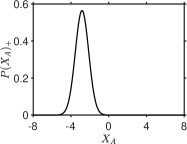
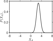
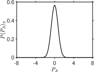
Figure 1: Top: Plots of $P(X_{A})_{\pm}$ and $P(P_{A})_{\pm}$ for the system $A$ at time $t_{3}$, when which-way information is present. The $P(P_{A})_{\pm}$ show no fringes. Here, $\alpha=\beta=2$.

On the other hand, one may take $t_{a}=t_{3}$ and $t_{b}=0$, so that there is no local unitary intertaction at $B$. Alternatively, one may evolve both sites according to $t_{a}=t_{b}=t_{3}$, and then perform a local unitary transformation $U_{B}(t_{2})^{-1}=(U_{\pi/4}^{(B)})^{-1}$ at $B$, to transform the system $B$ “back” to the initial state of $B$ at time $t_{1}$. Which-way information about $A$ at $t_{3}$ is then absent. The state of the combined systems at this time $t_{4}>t_{3}$ is

$$|\psi(t_{4})\rangle = \mathcal{N}\{U_{\pi/4}^{(A)}|\alpha\rangle|-\beta\rangle-U_{\pi/4}^{(A)}|-\alpha\rangle|\beta\rangle\}$$ (9)

If the final stage of the spin measurement $B$ is made at time $t_{4}$, the result will give either $S^{(B)}(t_{4})=1$ or $-1$. From the anti-correlation of (2), $S^{(B)}(t_{4})$ is interpreted as a measurement of the initial value of $-S_{1}^{(A)}$, and hence knowledge of that state of system $A$ at that time, $t_{1}$. If the outcome of $S^{(B)}(t_{4})$ is $\mp 1$ then, assuming the limit where $|-\beta\rangle$ and $|\beta\rangle$ are orthogonal states (i.e. large $\beta$), the system $A$ is projected into the superposition state

$$U_{\pi/4}|\pm\alpha\rangle=e^{-i\pi/4}\{\cos\pi/4|\pm\alpha\rangle+i\sin\pi/4|\mp\alpha\rangle\}$$ (10)

This is the state of the local system $A$ at time $t_{2}$ (see eqn (7)), conditioned on the initial state of $A$ at time $t_{1}$ being $|\pm\alpha\rangle$. Thus, if one measures $P(P_{A})$ conditional on the result of $-S^{(B)}(t_{4})=S_{1}^{(A)}$, the fringes are recovered. We find

$$P(P_{A})_{\pm}=\frac{e^{-P_{A}^{2}}}{\sqrt{\pi}}\{1\mp\sin(2\sqrt{2}P_{A}|\alpha|)\}$$ (11)

where $P(P_{A})_{+}$ and $P(P_{A})_{-}$ is the distribution for $P_{A}$ conditional on the result $+1$ or $-1$ for $S_{1}^{(A)}$, respectively. The distributions (Figure 2) show fringes, indicative of the system $A$ at time $t_{3}$ being in the superposition (10), and indicative of the loss of which-way information.

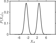
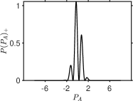
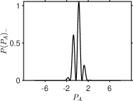
Figure 2: Top: Plots of $P(X_{A})_{\pm}$ and $P(P_{A})_{\pm}$ of the system $A$ at time $t_{2}$, where the outcome for $S_{4}^{(B)}=S_{A}^{(1)}$ is (left) $+1$, and (right) $-1$. The which-way information is lost, and the system $A$ is in the superposition (10). Here, $\alpha=\beta=2$.

The accurate calculation of the conditional probabilities $P(P_{A})_{\pm}$, without the simplistic assumption of a projection into a definite coherent state at $A$ on measurement at $B$, gives

$$P(P_{A})_{\pm} =\frac{2\mathcal{N}^{2}e^{-P_{A}^{2}}}{\sqrt{\pi}}\biggr{\{}1-e^{-2|\beta|^{2}}\cos(2\sqrt{2}P_{A}|\alpha|)$$

$$\mp\sin(2\sqrt{2}P_{A}|\alpha|)erf(\sqrt{2}|\beta|)\biggl{\}}$$ (12)

where $erf$ is the error function. The plots are indistinguishable from those of the approximate result for $\beta>1$, the limit $\beta\rightarrow\infty$ being the limit of an ideal measurement. The calculations in Figures 1 and 2 are based on evaluation of the joint distribution $P(P_{A},X_{B})$ (refer to macro-bell-lg ).

III.2 Interpretation in terms of wMR

As summarised in the Introduction, the delayed choice experiment has been interpreted as suggesting retrocausality. The decision to observe either the particle-like behaviour (which-way information) or the wave-like behaviour (fringes) of system $A$ is made at the later time $t_{4}$ (at $B$). This appears to retrospectively change the system $A$ at time $t_{3}$ from being in “one or other state” ($\varphi_{1}$ or $\varphi_{2}$; $|\alpha\rangle$ or $|-\alpha\rangle$) to being “in both states” (since the observation of fringes in $P(P_{A})$ is often interpreted to suggest the system $A$ was in “both states”, $|\alpha\rangle$ and $|-\alpha\rangle$). As explained in delayed-choice-causal-model-chaves , there is no requirement to assume retrocausality for the MZ delayed-choice experiment. The experiment described for cat states maps onto the qubit experiment for large $\alpha$, $\beta$, and gives a similar conclusion for the macroscopic qubits.

The macroscopic version of the quantum eraser is informative, because with the introduction of the macroscopic hidden variable, $\lambda_{i}$, it allows us to separate the macroscopic from the microscopic behavior. We consider compatibility with the assumption of weak macroscopic realism (wMR) $-$ that the system $A$ at the time $t_{2}$ is in a state with a definite value $\lambda_{3}^{(A)}$ which corresponds to the outcome of a measurement $S_{3}^{(A)}$, should it be performed. Here, there is no attempt to define the quantum state associated with that predetermination, so that predictions for other more microscopic measurements (and hence other hidden variables that determine those predictions) are not relevant. Thus, wMR does not postulate that the system is in one or other state $|\alpha\rangle$ or $|-\alpha\rangle$. In fact, we see there is no negation of wMR, because the fringes are only evident at the microscopic level of $\hbar$ (here $\hbar\sim 1$). The gedanken experiment is consistent with wMR. In that sense, the system always displays a particle-like behaviour.

The assumption of weak macroscopic realism (wMR) if applied to the double-slit experiment would be that the particle has a position constraining it to go through a definite slit even when fringes are observed (provided the slit does not restrict the position to of order $\hbar$ or less). For the definition of wMR, the predictions for other more precise position or momentum measurements of order $\hbar$ are not relevant. A similar interpretation of wMR for the MZ experiment is that the photon/ particle takes one or other path with a macroscopic uncertainty, but is not defined to be in one or other state $|+\rangle_{a,2}$ and $|-\rangle_{a,2}$.

The interpretation based on wMR suggests a lack of completeness of the description at the microscopic level. This can be clarified further. Indeed, if wMR holds, then it is possible to show that EPR-type paradoxes exist at the microscopic level. The EPR-type arguments indicate an incompleteness of a quantum state description if compatible with wMR, as explained in manushan-bell-cat-lg , and will be discussed further in Section VI.

IV Delayed-choice Leggett-Garg test of macrorealism

In this section, we consider the delayed choice experiment in the form of a Leggett-Garg test of macrorealism using entangled cat states. The advantage of the Leggett-Garg test is that all relevant measurements are macroscopic, distinguishing between the two macroscopically distinct coherent states. This contrasts with the quantum eraser proposal, where the paradoxical effects are inferred by the measurement of finely resolved fringes.

IV.1 Set-up

At time $t_{1}$, the system is prepared in the entangled cat state $|\psi_{Bell}(t_{1})\rangle$ of eqn (2). The spatially separated systems $A$ and $B$ dynamically evolve according to the unitary interactions (5) where $k=4$. We consider three times $t_{1}=0$, $t_{2}=\pi/4\Omega$ and $t_{3}=\pi/2\Omega$ (Figure 3). If the system at $A$ were prepared in a coherent state $|\alpha\rangle$, then at the later time $t_{a}=t_{2}=\pi/4\Omega$, the state of the system $A$ at time $t_{2}$ is in the asymmetric superposition manushan-cat-lg ; macro-bell-lg ; manushan-bell-cat-lg

$$U_{\pi/8}^{(A)}|\alpha\rangle = e^{-i\pi/8}\{\cos\pi/8|\alpha\rangle+i\sin\pi/8|-\alpha\rangle\}$$

where $U_{\pi/8}^{(A)}=U_{A}(\pi/4\Omega)$. A similar transformation $U_{\pi/8}^{(B)}$ is defined at $B$ for $t_{b}=t_{2}=\pi/4\Omega$. If one evolves for a time of $t_{2}=\pi/4\Omega$ at both sites, then the final state is

$$|\psi_{Bell}(t_{2},t_{2})\rangle = U_{\pi/8}^{(A)}U_{\pi/8}^{(B)}|\psi_{Bell}(t_{1})\rangle$$

$$= \mathcal{N}e^{-i\pi/4}(|\alpha\rangle|-\beta\rangle-|-\alpha\rangle|\beta\rangle)$$

The values of the macroscopic spins after the interaction time $t_{2}$ at each site are denoted $S_{2}^{(A)}$ and $S_{2}^{(B)}$. The spin $S_{2}^{(A)}$ of system $A$ can be inferred by measuring $S_{2}^{(B)}$ which is anticorrelated with the spin at $A$.

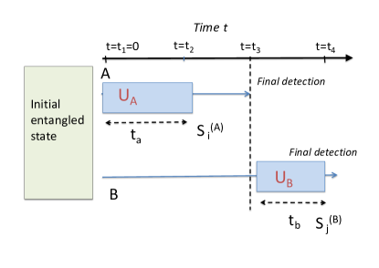
Figure 3: Sketch of the set-up for the delayed choice Leggett-Garg test. The system is prepared in the two-mode entangled cat state $|\psi_{Bell}(t_{1})\rangle$ at the time $t_{1}=0$, with the modes spatially separated. Independent local unitary interactions $U_{A}$ and $U_{B}$ take place at sites $A$ and $B$ respectively, with time settings $t_{a}$ and $t_{b}$. The times at $A$ are selected as either $t_{a}=t_{2}=\pi/4\Omega$ or $t_{a}=t_{3}=\pi/2\Omega$ and the final detection enables measurement of $S_{2}^{(A)}$ or $S_{3}^{(A)}$ respectively. At $B$, one selects either $t_{b}=t_{1}=0$ or $t_{b}=t_{2}=\pi/4\Omega$, the final detection enabling measurement of $S_{1}^{(B)}$ or $S_{2}^{(B)}$. The outcomes of $S_{1}^{(B)}$and $S_{2}^{(B)}$ are anticorrelated with the outcomes of $S_{1}^{(A)}$ and $S_{2}^{(A)}$ respectively, if measured. In the delayed choice experiment, the interaction at $B$ is delayed until after the final detection at $A$, at time $t_{3}$. Hence, the measurement of $S_{1}^{(B)}$ (or $S_{2}^{(B)}$) allows inference of the past value of $S_{1}^{(A)}$ (or $S_{2}^{(A)}$).

On the other hand, one may choose to evolve at $A$ for a time $t_{a}=t_{2}=\pi/4\Omega$, but not at the site $B$, so that $t_{b}=0$. The state after these interactions is

$$|\psi(t_{2},t_{1})\rangle = \mathcal{N}\{U_{\pi/8}^{(A)}|\alpha\rangle|-\beta\rangle-U_{\pi/8}^{(A)}|-\alpha\rangle|\beta\rangle\}$$

If the final readout stage of the spin measurement $B$ is made at time $t_{4}$ (Figure 3), the result will give a value $S^{(B)}(t_{4})\equiv S_{1}^{(B)}=\pm 1$. From $|\psi_{Bell}(t_{1})\rangle$ (eqn (2)), the value of $S^{(B)}(t_{4})$ is anticorrelated with the initial value of $S_{1}^{(A)}$, if we had chosen $t_{a}=t_{1}=0$. Therefore the measurement at $B$ is interpreted as a measurement of $S_{1}^{(A)}$. If the outcome of $S^{(B)}(t_{4})$ is $\mp 1$ then (assuming $|\beta\rangle$ and $|-\beta\rangle$ are orthogonal) from (9) we see that the system $A$ is reduced to the superposition state

$$U_{\pi/8}|\pm\alpha\rangle=e^{-i\pi/8}\{\cos\pi/8|\pm\alpha\rangle+i\sin\pi/8|\mp\alpha\rangle\}$$ (16)

This is the state of the local system $A$ at time $t_{2}$ (see eqn (7)), conditioned on the initial state of $A$ at time $t_{1}$ being $|\pm\alpha\rangle$. The value of $S_{2}^{(A)}$ can be measured directly at $A$. This combination of interactions therefore allows measurement of both $S_{2}^{(A)}$ and $S_{1}^{(A)}$.

Alternatively, we may evolve the system $A$ for a time $t_{a}=t_{3}=\pi/2\Omega$, while not evolving at $B$ ($t_{b}=t_{1}=0$). This gives

$$|\psi(t_{3},t_{1})\rangle = \mathcal{N}\{U_{\pi/4}^{(A)}|\alpha\rangle|-\beta\rangle-U_{\pi/4}^{(A)}|-\alpha\rangle|\beta\rangle\}$$

where $U_{\pi/4}|\pm\alpha\rangle$ is given by eqn (7). The spin $S_{3}^{(A)}$ can be measured directly at $A$. Measurement of $S^{(B)}(t_{4})\equiv S_{1}^{(B)}$ at $B$ gives the inferred result for the measurement $S_{1}^{(A)}$. This allows measurement of both $S_{3}^{(A)}$ and $S_{1}^{(A)}$.

Alternatively, one may select $t_{b}=t_{2}=\pi/4\Omega$ at $B$. According to (LABEL:eq:qe-1), the measurement at $B$ then allows measurement of $S_{2}^{(A)}$. If one evolves at $A$ for a time $t_{a}=t_{3}=\pi/2\Omega$, then this combination of interactions allows measurement of both $S_{2}^{(A)}$ and $S_{3}^{(A)}$.

The set-up (Figure 3) allows for a delayed choice of the measurement of either $S_{1}^{(A)}$ or $S_{2}^{(A)}$, by delaying the choice at $B$ to measure either $S_{1}^{(B)}$ or $S_{2}^{(B)}$. This amounts to a delay in the choice to interact the system $B$ for a time $t_{b}=0$, or else to interact system $B$ for a time $t_{b}=t_{2}$. This choice can be delayed until a time well after the time $t_{3}$, and well after the final detection (given by the measurement and readout of $X_{A}$) takes place at $A$.

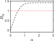
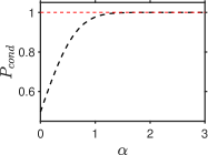
Figure 4: Violation of the Leggett-Garg inequality (18). We plot $B_{lg}=-\{\langle S_{1}^{(B)}S_{2}^{(A)}\rangle-\langle S_{1}^{(B)}S_{3}^{(A)}\rangle+\langle S_{2}^{(B)}S_{3}^{(A)}\rangle\}$ versus $\alpha$ for the state $|\psi_{Bell}(t_{1})\rangle$ (2), with $\beta=2$. Violation is obtained when $B_{lg}>1$. The verification of $\langle S_{i}^{(A)}S_{j}^{(A)}\rangle=-\langle S_{i}^{(B)}S_{j}^{(A)}\rangle$ for $i=1,2$ is given by the conditional distribution $P_{cond}$ defined as $P_{cond}=P(S_{i}^{(A)}=1|S_{i}^{(B)}=-1)$ as shown.

IV.2 Leggett-Garg inequality and violations

We now summarise the Leggett-Garg test of macrorealism for this system manushan-bell-cat-lg . The definition of macrorealism involves two assumptions: macroscopic realism and noninvasive measurability (NIM). For our purposes, we take the definition of macroscopic realism to be that of weak macroscopic realism (wMR) defined in the Introduction: This asserts that the system given by (1) is in a state with a definite prediction for the macroscopic spin $S^{(A)}$, $+1$ or $-1$. The system can then be assigned the hidden variable $\lambda$, the value of $\lambda$ being $+1$ or $-1$, which determines the result of the measurement $S^{(A)}$ should it be performed. Macrorealism also implies NIM, that the value of $\lambda$ can be measured with negligible affect on the subsequent macroscopic dynamics of the system.

For measurements of spin $S_{j}^{(A)}$ made on a single system $A$ at consecutive times $t_{1}<t_{2}<t_{3}$, macrorealism implies the Leggett-Garg inequality weak-solid-qubits-williams-jordan ; jordan_kickedqndlg2-2 ; legggarg-1

$$B_{lg}={\color[rgb]{0,0,0}{\color[rgb]{0,0,0}\langle S_{1}^{(A)}S_{2}^{(A)}\rangle+\langle S_{2}^{(A)}S_{3}^{(A)}\rangle-\langle S_{1}^{(A)}S_{3}^{(A)}\rangle}\leq 1}$$ (18)

As shown in manushan-bell-cat-lg ; macro-bell-lg , the cat system of Section IV.A is predicted to violate this inequality (Figure 4), meaning that macrorealism is falsified. While other Leggett-Garg inequalities have been proposed (e.g. nst ; halliwell-lg-multidimension ; legggarg-1 ), this particular inequality is useful where measurements are made on entangled subsystems. The approach we give in this paper uses spatial separation and delayed-choice to justify noninvasiveness, since the measurements of $S_{1}^{(A)}$ and $S_{2}^{(A)}$ can be made on system $B$. The approach can be applied to other macroscopic superposition states, such as NOON states noon-dowling ; bognoon-1 using the local unitary interaction given in macro-bell-lg . We comment that violations of Leggett-Garg inequalities have been predicted and tested for a range of superposition states (e.g. emary-review ; experiment-lg-2 ; lgexpphotonweak-1-2 ; goggin-1 ; massiveosci-1-1-1 ; Mitchell-1-1 ; lauralg-1 ; leggett-garg-recent-1 ; halliwell-leggett-garg-double-slit ; pan-leggett-garg-weak-value-interference-exp ; NSTmunro-1-1 ; dressel-bell-hybrid ) and alternative procedures exist to justify NIM.

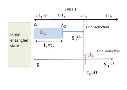
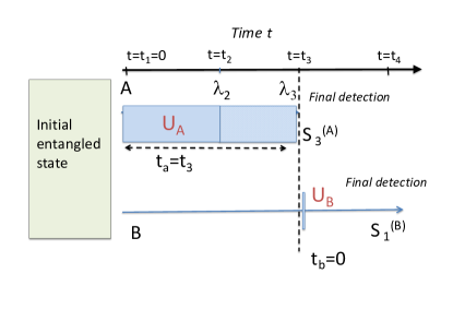
Figure 5: Sketch of the set-up for the delayed choice Leggett-Garg test. Notation is as for Figure 3. The top (lower) sketch shows measurement of $\langle S_{2}^{(A)}S_{1}^{(B)}\rangle$ ($\langle S_{3}^{(A)}S_{1}^{(B)}\rangle$). These measurements give the values of $\langle S_{2}^{(A)}S_{1}^{(A)}\rangle$ and $\langle S_{3}^{(A)}S_{1}^{(A)}\rangle$, based on the anticorrelation $S_{1}^{(B)}=-S_{1}^{(A)}$. For this measurement, there is no unitary interaction (rotation) at $B$. The predictions for the relevant distributions are given in Figure 7 (top). The results here are indistinguishable from those of an initial non-entangled state $\rho_{mix}$ (compare Figure 8 (top)).

We summarise the measurements enabling a test of the inequality (18), as in Figures 5 and 6. As we have seen, the value of $S_{1}^{(A)}$ or $S_{2}^{(A)}$ of system $A$ can be inferred noninvasively by measurement of the anti-correlated spin $S_{1}^{(B)}$ or $S_{2}^{(B)}$. The result for the moment $\langle S_{1}^{(A)}S_{2}^{(A)}\rangle$ is determined by a direct measurement of $S_{2}^{(A)}$ at time $t_{2}$, and an inferred measurement of $S_{1}^{(A)}$ by measuring $S_{1}^{(B)}$ at $B$ (Figure 5). The moment $\langle S_{1}^{(A)}S_{3}^{(A)}\rangle$ is measured similarly (Figure 5).

The quantum prediction for $\langle S_{1}^{(A)}S_{2}^{(A)}\rangle$ is based on the assumption that the measurement of $S_{1}^{(B)}$ projects the system $A$ into one or other state, $|\alpha\rangle$ or $|-\alpha\rangle$. The prediction is then $\langle S_{1}^{(A)}S_{2}^{(A)}\rangle=\cos(\pi/4)$, based on the evolution time of $t_{2}$ at $A$ (see eqn (16)). The moment $\langle S_{1}^{(A)}S_{3}^{(A)}\rangle$ is evaluated similarly, and from eqn (7) we see the prediction is $\langle S_{1}^{(A)}S_{3}^{(A)}\rangle=\cos(\pi/2)=0$.

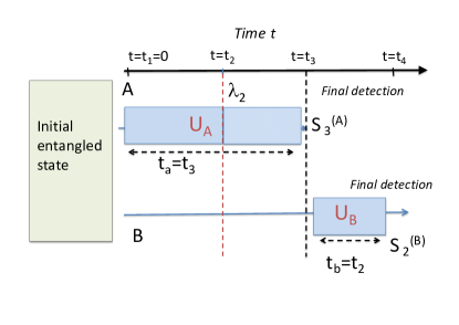
Figure 6: Sketch of the set-up for the Leggett-Garg test. Notation is as for Figure 3. The sketch depicts measurement of $\langle S_{3}^{(A)}S_{2}^{(B)}\rangle$, which based on the anticorrelation $S_{2}^{(B)}=-S_{2}^{(A)}$ gives the value for $\langle S_{3}^{(A)}S_{2}^{(A)}\rangle$. The predictions for the relevant distributions are given in Figure 7 (lower). The results at time $t_{4}$ are macroscopically different from those obtained if the state at time $t_{2}$ is non-entangled (compare Figure 8 (lower)). The results are inconsistent with local hidden variable models and the premise of deterministic macroscopic realism.

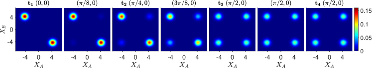
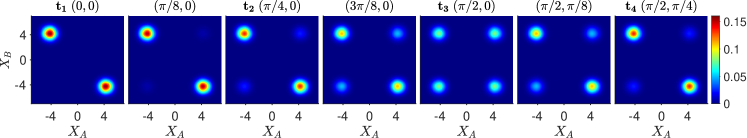
Figure 7: Contour plots of $P(X_{A},X_{B})$ showing the dynamics as the state $|\psi_{Bell}(t_{1})\rangle$ evolves through the three measurement sequences of the Leggett-Garg test in the delayed-choice gedanken experiment depicted in Figures 5 and 6. Here, we go from time $t=t_{1}$ (far left), through to $t=t_{2}$ (third picture from left), $t=t_{3}$ (fifth picture from left) and, finally, $t=t_{4}$ (far right). The systems evolve locally according to $H_{NL}^{(A/B)}$ for interaction times $t_{a}$ and $t_{b}$ given by $(t_{a},t_{b})$ in units of $\Omega^{-1}$. Top: The sequence to infer $S_{1}^{(A)}$ by delayed measurement of $S_{1}^{(B)}$, enabling measurement of $\langle S_{1}^{(B)}S_{3}^{(A)}\rangle=-\langle S_{1}^{(A)}S_{3}^{(A)}\rangle$ (final picture), as in Figure 5 (lower). The sequence to measure $\langle S_{1}^{(B)}S_{2}^{(A)}\rangle=-\langle S_{1}^{(A)}S_{2}^{(A)}\rangle$ uses $t_{a}=t_{2}=\pi/4$ as in Figure 5 (top) and ends with the third picture of the sequence. Lower: The sequence to infer $S_{2}^{(A)}$ by measurement of $S_{2}^{(B)}$, enabling measurement of $\langle S_{2}^{(B)}S_{3}^{(A)}\rangle=-\langle S_{2}^{(A)}S_{3}^{(A)}\rangle$ (final picture) as in Figure 6. Here, $t_{1}=0$, $t_{2}=\pi/4$ and $t_{3}=\pi/2$. $\alpha=\beta=3$.

For $\langle S_{2}^{(A)}S_{3}^{(A)}\rangle$, one would measure $S_{2}^{(B)}$ to determine the anticorrelated $S_{2}^{(A)}$, and measure $S_{3}^{(A)}$ directly at $A$ (Figure 6). The prediction for $\langle S_{2}^{(A)}S_{3}^{(A)}\rangle$ is based on the assumption that the system $A$ is in either $|\alpha\rangle$ or $|-\alpha\rangle$, at time $t_{2}$ (or else, that the measurement of $S_{2}^{(B)}$ projects $A$ to one of these states). The subsequent evolution for a time $\Delta t=\pi/8$ then leads to the prediction of $\langle S_{2}^{(A)}S_{3}^{(A)}\rangle=\cos(\pi/4)$ (refer eqn (LABEL:eq:state3-3)). This gives violation of the inequality (18), the left side being $\sqrt{2}$.

The above calculations assume large $\beta$ (and hence orthogonal $|\beta\rangle$ and $|-\beta\rangle$) so that one may justify the assumption that the system $A$ at times $t_{1}$ and $t_{2}$ is projected into one or other of the states $|\alpha\rangle$ or $|-\alpha\rangle$ once the measurement at $B$ is performed. To evaluate accurately requires evaluation of the joint distributions $P(X_{A},X_{B})$ for the different times of interaction $t_{a}$ and $t_{b}$. For large $\alpha$ and $\beta$, the simplistic result is indeed recovered, for all $\alpha,$$\beta>1$. The precise results were calculated in manushan-bell-cat-lg , and are given in Figures 4. The results agree with the moments above, predicting violation of the inequality, for $\alpha>1$. The plots of $P(X_{A},X_{B})$ for the various times of evolution are given in Figure 7.

The violation of the inequality (18) implies falsification of macrorealism. We note that the measurements $S_{i}^{(A)}$and $S_{j}^{(B)}$ are macroscopic in the sense that one needs only to distinguish between the two macroscopically separated peaks of the distributions $P(X_{A},X_{B})$ (Figure 7). Here, the meaning of “macroscopic” refers to a separation in phase space of quadrature amplitudes $X$ by an arbitrary amount ($\alpha\rightarrow\infty$).

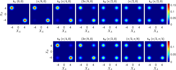
Figure 8: Contour plots of $P(X_{A},X_{B})$ showing the dynamics as the non-entangled state $\rho_{mix}$ evolves through the same measurement sequences given in Figure 7. Notation as for Figure 7. Top: The sequence evolves as in Figure 5 (lower) with a unitary rotation at site $A$ only. Athough starting with $\rho_{mix}$ at time $t_{1}$, the sequence is indistinguishable from that given by the top sequence in Figure 7 for the entangled state $|\psi_{Bell}(t_{1})\rangle$. Lower: We assume the system evolves as for Figure 6 and the lower sequence of Figure 7 with two unitary rotations, one at $A$ and one at $B$, but starting from a nonentangled state $\rho_{mix}$ at the time $t=t_{2}$. Although indistinguishable at the initial time $t_{2}$, the final picture at $t=t_{4}$ ($(\pi/2,\pi/4)$) differs macroscopically from that of the entangled state (compare with the lower sequence in Figure 7).

IV.3 Interpretation without macroscopic retrocausality

As explained above, macrorealism involves two assumptions: weak macroscopic realism (wMR) and noninvasive measurability. If we assume the validity of wMR, then we would conclude that noninvasive measurability fails: the measurement of the spin $S_{i}^{(B)}$ of $B$ disturbs the result for the spin $S_{j}^{(A)}$of $A$ ($j>i$). However, since the measurements are made at $B$ after the state of $A$ at the time $t_{3}$ is measured, this conclusion would seem to suggest a macroscopic retrocausal effect, where which measurement is made at $B$ alters the past value of $\lambda_{i}$ at $A$. In Section IV, we rigorously clarify the nature of this apparent retrocausality, by examining the dimension witness test proposed in delayed-choice-causal-model-chaves .

Here, we examine further, by analysing how the dynamics pictured in Figure 7 provides an interpretation that avoids the conclusion of macroscopic retrocausality. First, it is useful to compare with the dynamics of a non-entangled state (Figure 8)

$$\rho_{mix}=\frac{1}{2}\{|\alpha\rangle|-\beta\rangle\langle\alpha|\langle-\beta|+|-\alpha\rangle|\beta\rangle\langle-\alpha|\langle\beta|\}$$ (19)

The non-entangled cat state is consistent with the first Leggett-Garg premise of weak macroscopic realism (wMR), since each system can be viewed as being in one or other of two macroscopically distinct coherent states at time $t_{1}$. We first note that there is no distinguishable difference between the predictions $P(X_{A},X_{B})$ for the entangled ($|\psi_{Bell}(t_{1})\rangle$) and non-entangled ($\rho_{mix}$) states, at the level of the macroscopic outcomes (compare the first plot of the top sequences in Figures 7 and 8). A distinction exists, but at order $\hbar e^{-|\alpha|^{2}}$, invisible on the plots.

It is seen that where one measures $S_{1}^{(B)}$, the predictions $P(X_{A},X_{B})$ for the two systems beginning with the entangled ($|\psi_{Bell}(t_{1})\rangle$) and non-entangled ($\rho_{mix}$) states remain indistinguishable (compare the top sequences of Figures 7 and 8). This corresponds to there being no rotation (unitary evolution) at site $B$ (Figure 5). A distinction in fact exists, but this is at the microscopic level of order $\hbar e^{-|\alpha|^{2}}$, invisible on the plots manushan-bell-cat-lg .

There is a macroscopic difference however for the evolution where one measures $S_{2}^{(B)}$, which involves two unitary rotations after $t_{2}$, one at each site, as depicted in Figure 6. This is seen by comparing the lower sequences of Figure 7 and Figure 8. Here, if one starts with a non-entangled state $\rho_{mix}$ at time $t_{2}$ (Figure 8 (lower)), then even though the joint probabilities $P(X_{A},X_{B})$ are indistinguishable at $t_{2}$, the joint probabilities differ macroscopically after the evolution involving rotations at both sites (compare the last pictures in the lower sequences).

We conclude that the violation of macrorealism and the apparent retrocausality arises from the measurement of $\langle S_{2}^{(A)}S_{3}^{(A)}\rangle$, as depicted in Figure 6. The scenario of Figure 5 is consistent with macrorealism, since it can be modelled by evolution of $\rho_{mix}$.

IV.3.1 Weak macroscopic realism: the pointer measurement

To interpret without macroscopic retrocausality, we aim to show consistency with the assumption of weak macroscopic realism (wMR). We first examine this assumption more closely, along the lines given in manushan-bell-cat-lg .

Let us suppose the systems $A$ and $B$ are prepared at a time $t_{j}$ in a macroscopic superposition $|\psi_{pointer}\rangle$ of states with definite outcomes for pointer measurements $\hat{S}_{j}^{(A)}$ and $\hat{S}_{j}^{(B)}$. In this paper, the example of such a superposition is

$$|\psi_{Bell}\rangle=\mathcal{N}(|\alpha\rangle|-\beta\rangle-|-\alpha\rangle|\beta\rangle)$$ (20)

where $\alpha,$$\beta\rightarrow\infty$. The premise wMR asserts that the system $A$ at the time $t_{j}$ is in one or other of two macroscopic states $\varphi_{+}$ and $\varphi_{-}$, for which the result of the spin measurement $S_{j}^{(A)}$ (given by the sign of the coherent amplitude) is determined to be $+1$ or $-1$ respectively. Hence, the system $A$ at time $t_{j}$ may be described by the macroscopic hidden variable $\lambda_{j}^{(A)}$. The value of $\lambda_{j}^{(A)}$ is fixed as either $+1$ or $-1$ at the particular time $t_{j}$, prior to the pointer measurement, and is independent of any future measurement. By the pointer measurement, it is meant that the measurement can be made as a final quadrature detection, $X_{A}$, with no further unitary rotation $U_{A}$ necessary. Weak macroscopic realism does not mean that prior to the measurement of spin $S^{(A)}$ the system is in the state $|\alpha\rangle$ or $|-\alpha\rangle$, or indeed in any quantum state $-$ since the quantum states are microscopically specified, giving predictions for all measurements that might be performed on $A$. For the entangled state $|\psi_{Bell}\rangle$, similar assumptions apply to system $B$.

For the bipartite system depicted in Figures 5 and 6, wMR is to be consistent with a form of macroscopic locality. “Macroscopic locality of the pointer” was summarised in manushan-bell-cat-lg and asserts that the value of the macroscopic hidden variable $\lambda_{j}^{(A)}$ for the system $A$ cannot be changed by any spacelike separated event, or measurement at the system $B$ that takes place at time $t\geq t_{j}$ e.g. it cannot be changed by a future event at $B$. In this interpretation, the system $A$ at each time $t_{i}$ ($i=1,2,3$) is in one or other of states $\varphi_{i,+}$ or $\varphi_{i,-}$ with a definite value $+1$ or $-1$ of spin $S_{i}^{(A)}$. The premise “macroscopic locality of the pointer” is to be distinguished from the stronger assumption, macroscopic locality, introduced in manushan-bell-cat-lg . “Macroscopic locality” assumes locality to apply to spacelike-separated measurement events, but here the measurement setting for system $A$ is not necessarily established, so that $A$ is not necessarily prepared in the pointer basis. This allows for the possibility of a further unitary rotation at $A$, before the final detection of $X_{A}$. The premise of weak macroscopic realism is thus not contradicted by the violation of the macroscopic Bell inequalities reported in macro-bell-lg ; manushan-bell-cat-lg .

IV.3.2 Delayed collapse and unitary rotation at one site only: consistency with wMR

The dynamics indicates consistency with wMR. We focus on two features, explained in Ref. manushan-bell-cat-lg : delayed collapse and the single rotation.

Let us suppose that at the time $t_{j}$ the dynamics $U^{(A)}$ for a pointer measurement $S_{j}^{(A)}$ has taken place at $A$. The final detection (the “collapse” or “projection”) stage of the measurement $S_{j}^{(A)}$ at $A$ can be delayed for an infinite time, and there is no change in the macroscopic joint probabilities $P(X_{A},X_{B})$. The result is true even where there is a unitary rotation $U_{B}$ at the site $B$ after the time $t_{j}$: the joint probabilities $P(X_{A},X_{B})$ do not depend on whether the final detection at $A$ is before or after the unitary evolution $U_{B}$. The full calculations are given in manushan-bell-cat-lg and show that while there are differences in the final distributions, these differences are negligible, of order $\hbar e^{-|\alpha|^{2}}$. This supports the wMR assumption, that for the pointer measurement ($S_{j}^{(A)}$ in this case), the result is determined by $\lambda_{j}^{(A)}$ at the time $t_{j}$ $-$ we can consider $\lambda_{j}^{(A)}$ as fixed.

There is also consistency with wMR for the dynamics given by Figures 5 and 7 (top), where there is no unitary rotation at the site $B$ (after $t_{1}$). Comparing Figures 7 (top) and 8 (top), we see that the macroscopic dynamics of the sequences for $\langle S_{1}^{(B)}S_{3}^{(A)}\rangle$ and $\langle S_{1}^{(B)}S_{2}^{(A)}\rangle$, which involve only one unitary rotation (at $A$), are identical to those of the non-entangled state $\rho_{mix}$, and hence are consistent with wMR. The macroscopic probabilities for the sequences with a rotation at one site only are also consistent with those of a local hidden variable theory i.e. the final outcomes at $A$ and $B$ can be interpreted as being due to a local interaction at $A$.

IV.3.3 Failure of deterministic macroscopic realism: unitary rotation at both sites

The violations of the Leggett-Garg inequality can be shown to arise as a failure of deterministic macroscopic realism (dMR), as studied in manushan-bell-cat-lg ; macro-bell-lg . This premise (different to wMR) asserts a predetermined outcome for the measurement prior to the unitary rotation $U$ that determines the measurement setting. Where one has two unitary rotations, one at each site, after the time $t_{j}$, as in Figure 6, there is no longer consistency with the predictions of $\rho_{mix}$.

Let us consider the scenario of Figure 6, at time $t_{2}$. The value of $\lambda_{2}^{(A)}$ is predetermined according to wMR, for the pointer measurement $S_{2}^{(A)}$. However, one may also consider the outcome of a measurement $S_{3}^{(A)}$ at the later time, made by applying a rotation $U^{(A)}(\pi/4)$ and then measuring $X_{A}$. If we assume dMR, then this latter outcome can also be regarded as predetermined, and we can assign the hidden variable $\lambda_{3}^{(A)}$ to the system at the time $t_{2}$. Similarly, assuming dMR, one may assign variables $\lambda_{2}^{(B)}$ and $\lambda_{3}^{(B)}$ to system $B$, at time $t_{2}$.

Extending this argument, the premise dMR would imply simultaneous values for the outcomes at time $t_{1}$ regardless of the future unitary dynamics required to make the actual measurements, and would hence imply the Leggett-Garg inequality (18). Similarly, the macroscopic Bell inequality studied in macro-bell-lg ; manushan-bell-cat-lg would apply. We have show in Section IV.B that the Leggett-Garg inequality is violated, indicating failure of dMR. Similarly, the macroscopic Bell inequality derived in macro-bell-lg ; manushan-bell-cat-lg is violated. This implies that dMR is (predicted to be) falsified.

IV.3.4 Explanation

The apparent retrocausal effect can be explained as arising from the failure of deterministic macroscopic realism. The failure of dMR may also be viewed as a macroscopic Bell nonlocality, as discussed in manushan-bell-cat-lg ; macro-bell-lg . We argue however that the gedanken experiment is consistent with weak macroscopic realism.

We explain further. First, examining Figure 7 for the Leggett-Garg violations, we see that the macroscopic dynamics of the sequences for $\langle S_{1}^{(B)}S_{3}^{(A)}\rangle$ and $\langle S_{1}^{(B)}S_{2}^{(A)}\rangle$ (Figure 5) involving only one unitary rotation are identical to those of the non-entangled state $\rho_{mix}$, and hence are consistent with wMR. We next consider measurement of $\langle S_{2}^{(A)}S_{3}^{(A)}\rangle$. In measuring $\langle S_{2}^{(A)}S_{3}^{(A)}\rangle$ via $\langle S_{2}^{(B)}S_{3}^{(A)}\rangle$, as in the lower sequence of Figure 7, the system at $A$ is entangled with $B$ at time $t_{2}$. An interpretation consistent with wMR is possible, since the measurement of $\langle S_{2}^{(B)}S_{3}^{(A)}\rangle$ involves two rotations after the time $t_{2}$, one at $A$ and one at $B$ (as in Figure 6). This double rotation gives rise to macroscopic nonlocality (violations of a macroscopic Bell inequality ) i.e. to the failure of deterministic macroscopic realism macro-bell-lg ; manushan-bell-cat-lg .

Figure 9: Consistency with weak macroscopic realism is possible for the time sequence of Figure 6. The system at time $t_{1}$ has valid hidden variables $\lambda_{1}^{(A)}$ and $\lambda_{1}^{(B)}$, being indistinguishable from $\rho_{mix}$. At time $t_{2}$, system $A$ has valid $\lambda_{2}^{(A)}$ and $\lambda_{1}^{(A)}$, the value of $\lambda_{1}^{(A)}$ being given by the pointer measurement on $B$ at the time $t_{2}$. Similarly, system $B$ at time $t_{2}$ has valid $\lambda_{1}^{(B)}$ and $\lambda_{2}^{(B)}$. At time $t_{3}$, the system $A$ has valid $\lambda_{3}^{(A)}$ and $\lambda_{1}^{(A)}$, since the value of $\lambda_{1}^{(A)}$ can be given by the pointer measurement at $t_{3}$ on $B$. At time $t_{3}$, system $B$ has valid $\lambda_{1}^{(B)}$ and $\lambda_{3}^{(B)}$ (because $\lambda_{3}^{(B)}$ can be inferred from $\lambda_{3}^{(A)}$). At time $t_{4}$, system $A$ has valid $\lambda_{3}^{(A)}$ and $\lambda_{2}^{(A)}$.

The validity of weak macroscopic realism can then be argued as follows (Figure 9). Following Figure 6, the system $A$ at times $t_{1}$ and $t_{2}$ can indeed be represented by the hidden variables $\lambda_{1}^{(A)}$ and $\lambda_{2}^{(A)}$ (meaning that the pointer measurements of $S_{1}^{(A)}$ and $S_{2}^{(A)}$ have predetermined outcomes), because the predictions for pointer measurement $S_{1}^{(A)}$ and $S_{2}^{(A)}$ are identical with those arising from $\rho_{mix}$ (there has been a rotation at one site, $A,$ only). This is also true of the system $B$ at time $t_{1}$: it can be described by a $\lambda_{1}^{(B)}$, for the reason that the predictions are indistinguishable from those of $\rho_{mix}$.

At time $t_{2}$, $A$ can also be consistently represented by a hidden variable $\lambda_{1}^{(A)}$, because the value $S_{1}^{(B)}$ at $B$ is determinable by a pointer measurement, without further rotation. Also, because of the correlation with $S_{2}^{(A)}$, one would conclude $\lambda_{2}^{(B)}$ can be assigned to the state $B$ at the time $t_{2}$, because the outcome after the unitary evolution $U^{(B)}(\pi/4)$ is predetermined. However, it is not the case that at time $t_{2}$ the outcome of $S_{3}^{(A)}$ is predetermined (if $U^{(A)}(\pi/4)$ would be performed), because dMR fails. Hence, at time $t_{2}$, it is not true that the hidden variable $\lambda_{3}$ can be assigned to the state at $A$, because the unitary rotation $U^{(A)}(\pi/4)$ has not been performed. Regardless, this does not imply failure of wMR, because the dynamics associated with $U^{(A)}(\pi/4)$ is in the future of $t_{2}$.

On the other hand, if the unitary rotation $U^{(B)}(\pi/2)$ that precedes the measurement $S_{3}^{(B)}$ is performed prior to the time $t_{2}$ at $B$, then the state at $A$ at time $t_{2}$ can be assigned $\lambda_{3}^{(A)},$ but can no longer be assigned $\lambda_{1}^{A)}$ at that time $t_{2}$. This interpretation allows for macroscopic Bell nonlocal effects when there are unitary rotations at both sites, but is also consistent with weak macroscopic realism (wMR) and hence does not indicate macroscopic retrocausality.

V Dimension Witness test

We next follow the approach of Chaves, Lemos and Pienaar (CLP) delayed-choice-causal-model-chaves , by demonstrating violation of the dimension witness inequality Dimension-Witness-Brunner ; Quantum-Dimension-Witness ; bowles-dimension-test-exp ; ahrens-exp-dimension-test-nat-phys ; Yu-causal-model-exp ; delayed-choice-experiment-chaves . Here, one considers two-dimensional models and, within this framework, confirms the failure of all non-retrocausal models. Our results extend beyond those of CLP because the conclusions of retrocausality apply to the macroscopic qubits $|\alpha\rangle$ and $|-\alpha\rangle$ where $\alpha$ is large, for which the binary outcomes of the relevant measurements are distinguishable beyond $\hbar$. This test makes concrete the apparent retrocausality discussed in Section IV.C, and elucidates how this can be interpreted as due to the limitation of the assumption of two-dimensional hidden variable model.

We first consider the Wheeler-CLP delayed-choice experiment performed with tunable beam splitters i.e. with a variable reflectivity. A single boson is incident on the beam splitter, so that the input system is the two-mode state $|1\rangle_{a}|0\rangle_{b}$ (Figure 10). The two modes ($c$ and $d$) at the outputs of the beam splitter have boson operators

$$\hat{c} = \hat{a}\cos\theta-\hat{b}\sin\theta$$

$$\hat{d} = \hat{a}\sin\theta+\hat{b}\cos\theta$$ (21)

After the beam splitter, the state of the field in the interferometer is

$$|\psi\rangle_{p}=a^{\dagger}|0\rangle_{a}|0\rangle_{b}=\cos\theta|1\rangle_{c}|0\rangle_{d}+\sin\theta|0\rangle_{c}|1\rangle_{d}$$ (22)

This is the preparation state, prepared at time $t_{1}$. The fields pass through the interferometer, and are recombined at a second beam splitter to produce final output modes $e$ and $f$. The beam splitter transformation

$$\hat{e} = \hat{c}\cos\phi-\hat{d}\sin\phi$$

$$\hat{f} = \hat{c}\sin\phi+\hat{d}\cos\phi$$ (23)

constitutes the measurement, and gives the final state

$$|\psi\rangle_{m} = \cos(\theta-\phi)|1\rangle_{e}|0\rangle_{f}+\sin(\theta-\phi)|0\rangle_{e}|1\rangle_{f}$$ (24)

The binary outcomes $|1\rangle_{c}|0\rangle_{d}$ and $|0\rangle_{0}|1\rangle_{d}$ are denoted $b=1$ and $b=-1$ respectively. The expectation value for $b$ is $E(\theta,\phi)=\cos^{2}(\theta-\phi)-\sin^{2}(\theta-\phi)=\cos\left(2(\theta-\phi)\right)$. Certain choices of angles $\theta$ and $\phi$ will violate the dimension witness inequality, as we show below.

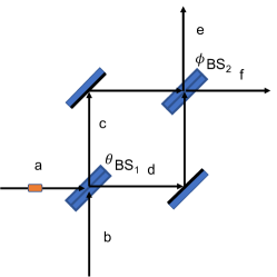
Figure 10: Schematic of Wheeler-CLP delayed choice experiment. A single boson two-mode state $|1\rangle_{a}|0\rangle_{b}$ is incident on the first beam splitter ($BS_{1}$). The first beam splitter introduces a variable reflectivity given by $\theta$ with output modes $c$ and $d$. These two modes are again recombined at a second beam splitter $BS_{2}$ to produce final output modes $e$ and $f$ with variable transformation angle $\phi$.

We map the above scheme onto a macroscopic system using the cat-state dynamics as shown by Figure 11. The input state is $|\alpha\rangle$. The nonlinear interaction $H_{NL}$ replaces the beam splitter, and for certain choices of interaction time $t_{\theta}=m\pi/8$ where $m$ is an integer prepares the system in the superposition

$$|\psi\rangle_{p}=e^{-i\varphi}(\cos\theta|\alpha\rangle+i\sin\theta|-\alpha\rangle)$$ (25)

where $\theta=t_{\theta}/2$ and $\varphi=t_{\theta}/2$ is a phase factor. This is proved in the Appendix C. The measurement stage corresponding to the second beam splitter consists of a second interaction $H_{NL}$ applied for a time $t_{\phi}$, so that

$$|\alpha\rangle\rightarrow|\alpha\rangle_{t}=e^{-i\varphi_{2}}(\cos\phi|\alpha\rangle+i\sin\phi|-\alpha\rangle)$$

$$|-\alpha\rangle\rightarrow|-\alpha\rangle_{t}=e^{-i\varphi_{2}}(\cos\phi|-\alpha\rangle+i\sin\phi|\alpha\rangle)$$ (26)

for certain choices of $\phi$. The final state after the interaction is

$$|\psi\rangle_{f} = e^{-iH_{NL}t_{\phi}/\hbar}|\psi\rangle_{p}$$ (27)

$$= e^{-i(\varphi+\varphi_{2})}(\cos\theta(\cos\phi|\alpha\rangle+i\sin\phi|-\alpha\rangle)$$

$$+i\sin\theta(\cos\phi|-\alpha\rangle+i\sin\phi|\alpha\rangle))$$

$$= e^{i\eta}(\cos(\theta+\phi)|\alpha\rangle+i\sin(\theta+\phi)|-\alpha\rangle)$$

where $\eta$ is a phase factor. Identifying $b=1$ as outcome $|\alpha\rangle$ and $b=-1$ as outcome $|-\alpha\rangle$, we obtain the results

$$E(\theta,\phi)=\cos(2(\theta+\phi))$$ (28)

similar to the modified Wheeler-CLP delayed choice experiment. It is emphasized that the expression for $E(\theta,\phi)$ is only true for certain values of $\theta$ and $\phi$, where (26) holds.

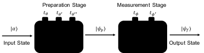
Figure 11: The set up for a macroscopic Wheeler-CLP delayed-choice experiment where we make use of the cat-state dynamics for a prepare and measure scenario. An initial input of $|\alpha\rangle$ undergoes a nonlinear interaction $H_{NL}$ for a time $t_{\theta}$ at the preparation stage of the system corresponding to the first beam splitter $BS1$. A second interaction $H_{NL}$ is applied for a time $t_{\phi}$ at the measurement stage which corresponds to the second beam splitter $BS2$. We make use of a dimension test on the final output to demonstrate failure of two-dimensional non-retrocausal models for the macroscopic system.

The set-up is an example of a prepare and measure scenario considered by CLP delayed-choice-causal-model-chaves . In their notation, the first measurement setting $t_{\theta}$ is denoted $\theta$ and the second $t_{\phi}$ is denoted by $\phi$. They derived a dimension witness inequality (DWI) that is satisfied for nonretrocausal models of no more than two dimensions. In our notation, this inequality for the preparation settings $\theta$, $\theta^{\prime}$, $\theta^{\prime\prime}$ and the measurement settings $\phi$, $\phi^{\prime}$ is

$$I_{DW}={\color[rgb]{0,0,0}{\color[rgb]{0,0,0}\Bigl{|}E(\theta,\phi)+E(\theta,\phi^{\prime})+E(\theta^{\prime},\phi)\ \ \ \ \ }}$$

$$-E(\theta^{\prime},\phi^{\prime})-E(\theta^{\prime\prime},\phi)\Bigr{|} \leq 3$$ (29)

where here $E(\theta,\phi)=\cos(2(\theta+\phi))$. The $t_{\theta}$ and $t_{\phi}$ denote the time settings at the respective beam splitter interactions $H_{NL}$. If we violate DWI, then this indicates failure of all non-retrocausal classical two-dimensional models, suggesting the implication of retrocausality if we are to view the system as observing a two-dimensional classical realist model. For a classical two-dimensional model, one would conclude that the choice of measurement $\phi$ affects the earlier state.

The inequality DWI (29) also follows from the assumptions of macrorealism. Let us suppose the system to be in one or other of two states $\varphi_{+}$ and $\varphi_{-}$ (such as $|\alpha\rangle$ and $|-\alpha\rangle$) that will give outcomes $+1$ and $-1$ for the measurement of the macroscopic value $S$ at the times $t_{p}$ and $t_{m}$. Here, $S$ is the sign of $X_{A}$, as defined in Sections III and IV. Then one may assign hidden variables $\lambda_{p}=\pm 1$ and $\lambda_{m}=\pm 1$ to the system at each of these times, the value $+1$ ($-1$) denoting that the outcome for $S$ will be $+1$ ($-1$) respectively. If we assume one may measure the value of $\lambda_{p}$ without affecting the value of $\lambda_{m}$ at the later time (and vice versa), then the expectation value defined as $E(\theta,\phi)=\langle\lambda_{p}\lambda_{m}\rangle$ will satisfy the DW inequality. This is readily proved by calculating the averages allowing for all possible combinations of values $\pm 1$ for $\lambda_{p}$ and $\lambda_{m}$.

It is known that for the solution $E(\theta,\phi)=\cos(2(\theta-\phi))$ given by eq. (28), violation of the DW inequality is possible, the maximum value for $I_{DW}$ being $I_{DW}=1+2\sqrt{2}=3.8284$. The angle choices are $\theta=\pi/8$, $\theta^{\prime}=3\pi/8$, $\theta^{\prime\prime}=-\pi/4$, $\phi=\pi/4$, $\phi^{\prime}=0$ delayed-choice-causal-model-chaves . In the macroscopic case where the solution is $E(\theta,\phi)=\cos(2(\theta+\phi))$, we select $\theta=\pi/8$, $\theta^{\prime}=3\pi/8$, $\theta^{\prime\prime}=7\pi/4$, $\phi=7\pi/4$, $\phi^{\prime}=0$. For these angle choices, the two-state solution (26) holds (refer Appendix C), as necessary for a macroscopic two-state test. The maximum violation $I_{DW}=1+2\sqrt{2}$ is possible for this angle choice. We may also select $\theta=\pi/4$, $\theta^{\prime}=\pi/2$, $\theta^{\prime\prime}=7\pi/8$, $\phi=13\pi/8$, $\phi^{\prime}=15\pi/8$.

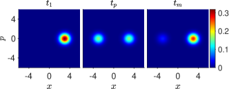
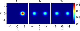
Figure 12: Contour plots for the $Q$ function $Q(x,p)$ as the system of Figure 11 evolves from the coherent state $|\alpha\rangle$ at time $t_{1}=0$. (Top) In this sequence, the first interaction $H_{NL}$ acts for a time $t_{2}=t_{\theta}$, preparing the system in the two-state superposition $|\psi\rangle_{p}$ (eq. (25)) at the time $t_{2}=t_{p}$. This is followed by a second interaction $H_{NL}$ for a time $t_{\phi}$ to produce a final state at time $t_{3}=t_{m}$. Here, $\theta=\pi/4$ and $\phi=-\pi/8$. (Lower) The lower sequence depicts the system prepared at the time $t_{p}$ in a mixture of states $|\alpha\rangle$ and $|-\alpha\rangle$. This occurs if the system is measured at that time, in such a way that the system collapses to the mixture. The system then evolves according to $H_{NL}$ for a time $t_{\phi}$ to produce the final state at time $t_{3}=t_{m}$.

In Figure 12, we plot the $Q$ function for the state of the system at the times $t_{0}$, $t_{p}$ and $t_{m}$. The $Q$ function is defined as

$$Q(x,p)=\frac{1}{\pi}\langle\alpha_{0}|\rho|\alpha_{0}\rangle$$ (30)

where $|\alpha_{0}\rangle$ is a coherent state, and $\alpha_{0}=x+ip$. The two-state dynamics is evident, as the system evolves under the action of $H_{NL}$. The $H_{NL}$ provides the rotation into the superposition state, in analogy to the beam splitter interaction. Also plotted in Figure 12 is the $Q$ function where the system at the time $t_{p}$ is prepared in a mixture of $|\alpha\rangle$ and $|-\alpha\rangle$. This applies where the system in the superposition at $t_{p}$ is measured, so that an experimentalist may determine which of the states the system was in at the time $t_{p}$. In fact, the $Q$ function for the superposition (top graph) differs from that of the mixture (lower graph) by terms of order $e^{-|\alpha|^{2}}$. For $\alpha>1$, this difference is not visually noticeable on the scale of the plots. It is noted however that after the subsequent rotation $H_{NL}^{\phi}$ ($\phi\neq 0$), the $Q$ functions provided from the superposition (top graph at time $t_{m}$) and the mixture (lower graph at $t_{m}$) are macroscopically distinguishable.

The $Q$ function $Q(x,p)$ corresponds to anti-normally ordered moments, and hence does not directly correspond to the measured probabilities for $x$ and $p$ at the microscopic level of $\hbar$. However, at the macroscopic level where one distinguishes between the two states $|\alpha\rangle$ and $|-\alpha\rangle$, the $Q$ function accurately depicts the relative probabilities i.e. the weighting of the two peaks as pictured in the plots corresponds to the relative probabilities for the binary outcomes, $b=1$ and $b=-1$. The extra terms of order $e^{-|\alpha|^{2}}$are negligible.

The violation of the dimension witness inequality indicates failure of two-dimensional non-retrocausal models. This is not inconsistent with the non-retrocausal interpretation given by Section IV.C, because the phase space dynamics relies on a continuum of values for $X$ and $P$. At time $t_{2}$ there is no distinction between the macroscopic depictions $Q(x,p)$ for the superposition and mixed state (compare also the pictures at $t_{2}$ for the lower sequences of Figures 7 and 8). Yet, there are differences of order $\hbar e^{-|\alpha|^{2}}$. It is due to these microscopic differences between the superposition (entangled) and mixed (non-entangled) states, evident in the full phase-space distribution at $t_{2}$, that there is a different dynamics, leading to a macroscopic difference in $E(\theta,\phi)$ at the later time $t_{3}$.

VI Weak macroscopic realism and EPR paradoxes at a microscopic level

In the previous sections, we show how to realise macroscopic paradoxes involving Leggett-Garg and dimension witness inequalities. While there is a contradiction between deterministic macroscopic realism (dMR) and quantum mechanics for these paradoxes, inconsistency with weak macroscopic realism (wMR) is not demonstrated at this macroscopic level. However, inconsistencies arise at the microscopic level.

In this section, we show that at a microscopic level where measurements resolve at the level of $\hbar$, the premises of wMR and local causality give EPR-type paradoxes epr-1 . This implies that there is inconsistency between each of these premises and the completeness of quantum mechanics. EPR paradoxes involving local causality have been illustrated previously for macroscopic superpositions of type laura-decoh-steer-josa ; macro-pointer-interpretation-jphysa

$$|\psi\rangle=\frac{1}{\sqrt{2}}(|\alpha\rangle|\uparrow\rangle+|-\alpha\rangle|\downarrow\rangle)$$ (31)

often taken as an example of a “Schrodinger cat” state cats-brune ; frowis-rmp ; cats-monroe-1 . The approach here is similar, since for large $\beta$, the coherent states $|\beta\rangle$ and $|-\beta\rangle$ are orthogonal qubits.

VI.1 EPR paradox using local causality

We consider the bipartite system prepared in the Bell state

$$|\psi_{Bell}\rangle=\frac{1}{\sqrt{2}}(|\alpha\rangle|-\beta\rangle-|-\beta\rangle|\alpha\rangle)$$ (32)

at time $t_{2}$, as for (8). The original EPR argument shows incompatability between the premise of local realism and the completeness of quantum mechanics epr-1 . The EPR argument was generalised to allow for imperfect correlation between the two sites in epr-reid-2 , including for spin systems in bohm-crit ; rmpepr-2 . Here, we apply this generalisation to illustrate the paradox for the entangled Bell cat state.

The EPR argument considers the prediction for $X_{A}$, given a measurement at $B$. A measurement of $S_{2}^{(B)}$ at $B$ will “collapse” system $A$ to the quantum state $|\alpha\rangle$ or $|-\alpha\rangle$, implying a variance $(\Delta X_{A})^{2}=1/2$ for $A$, conditioned on the result for $S_{2}^{(B)}$. We write this conditional variance as $\Delta_{inf}^{2}X_{A}\equiv(\Delta_{inf}X_{A})^{2}=1/2$, the variance for the inference of $X_{A}$ given the measurement at $B$.

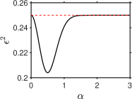
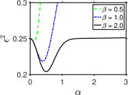
Figure 13: Plots showing the violation of the macroscopic EPR inequality (34). We first plot (left) $\mathcal{E}^{2}$ given by eqn (33). The same result is given for $\mathcal{E}_{M}^{2}$ which defined the macroscopic paradox, eq. (37). The second plot (right) shows the full calculation for $\mathcal{E}^{2}$ given by eqs. (LABEL:eq:var-epr-xfull) and (LABEL:eq:var-epr-pfull) based on the proposed method to measure $\beta$ using $X_{B}$, which assumes $\beta$ to be sufficiently large. Here, we show $\mathcal{E}^{2}$ versus $\alpha$ for $\beta=0.5$, $\beta=1$ and $\beta=2.$

The EPR argument then considers the prediction for $P_{A}$ of system $A$ at time $t_{2}$, as can be inferred from a measurement made at $B$. Here, we propose that the measurement made at $B$ be given by $U_{B}(t_{2})^{-1}$ followed by a measurement of $S_{2}^{(B)}$ (the sign of $\hat{X_{B}}$). The state after the transformation $U_{B}(t_{2})^{-1}$ is (9), and the measurement of $S_{2}^{(B)}$ allows an inference of the value of $P_{A}$, of system $A$ at time $t_{2}$. The measurement of $S_{2}^{(B)}$ at $B$ “collapses” system $A$ to either $U_{\pi/8}^{(A)}|\alpha\rangle$ or $U_{\pi/8}^{(A)}|-\alpha\rangle$. Following the method of epr-reid-2 , the inferred statistics is thus given by $U_{\pi/8}^{(A)}|\alpha\rangle$ or $U_{\pi/8}^{(A)}|-\alpha\rangle$, which are superpositions (10) of $|\alpha\rangle$ or $|-\alpha\rangle$, and for which the conditional distributions are $P_{+}(P_{A})$ and $P_{-}(P_{A})$ of eqn (11) respectively. These distributions show fringes, and have the variance $\Delta_{inf}^{2}P_{A}$ for $P$. This variance of the inferred value for $P_{A}$ is macro-pointer-interpretation-jphysa

$$\Delta_{inf}^{2}P_{A}=\frac{1}{2}-|\alpha|^{2}e^{-4|\alpha|^{2}}$$ (33)

The level of combined inference is

$$\varepsilon=\Delta_{inf}X_{A}\Delta_{inf}P_{A}<\frac{1}{2}$$ (34)

which is below the value for the uncertainty principle, $\Delta X_{A}\Delta P_{A}\geq\frac{1}{2}$, thus implying an EPR paradox epr-reid-2 .

It is also known that the observation of (34) demonstrates an EPR steering hw-1-2 ; eric-2 ; uola-steer-review . If Bell’s premise of local causality is assumed valid, the condition (34) is paradoxical because it implies that the system $A$ cannot be specified as being in any mixture of localised quantum states $\varphi_{+}$ or $\varphi_{-}$ (since such states would need to violate the uncertainty principle) hw-1-2 ; eric-2 ; uola-steer-review . This negates the hypothesis that the system of (32) can be regarded as being in either $|\alpha\rangle$ or $|-\alpha\rangle$ (or indeed in any $\varphi_{+}$ or $\varphi_{-}$ if these are to be quantum states) in a way that is consistent with local causality. The original EPR paradox assumes local realism, a more specific form of local causality useful when one has perfectly correlated results for both conjugate measurements.

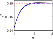
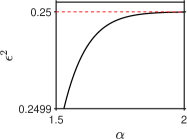
Figure 14: Plots showing the violation of the macroscopic EPR inequality (34). Notation as for Figure 13. Here, we give a close-up of results for the full calculation showing the cut-off values of $\beta$ needed for $\mathcal{E}^{2}<1/4$, for larger $\alpha$.

In the above prediction for the EPR inequality, it is assumed that an idealised measurement at $B$ “collapses” system $A$ into one or other of the coherent states. In a more rigorous analysis, we evaluate the conditional statistics for system $A$ using the specific proposal for the measurement at $B$, where the sign of $X_{B}$ is measured, as in the calculations of Section IV. This gives for the state (8) an inference variance in $X_{A}$ of

$$\Delta_{inf}^{2}X_{A} =\frac{1}{2}+\frac{2\left|\alpha\right|^{2}}{\left(1-e^{-2\left|\alpha\right|^{2}-2\left|\beta\right|^{2}}\right)}-\frac{2\left|\alpha\right|^{2}erf(\sqrt{2}\left|\beta\right|)^{2}}{\left(1-e^{-2\left|\alpha\right|^{2}-2\left|\beta\right|^{2}}\right)^{2}}$$

The full details are given in the Appendix. Similarly, the inferred variance for $P$ is calculated assuming the state (9). We find

$${\normalcolor{\normalcolor\Delta_{inf}^{2}P_{A}}} = {\color[rgb]{0,0,1}{\color[rgb]{0,0,0}\frac{1}{2}+}{\color[rgb]{0,0,0}\frac{2|\alpha|^{2}}{{\color[rgb]{0,0,0}\left(e^{2|\alpha|^{2}+2|\beta|^{2}}-1\right)}}-\frac{|\alpha|^{2}erf(\sqrt{2}|\beta|)^{2}}{\{e^{2|\alpha|^{2}}-e^{-2|\beta|^{2}}\}^{2}}}}$$

In the limit of large $\beta$, where the measurement becomes ideal, we see that $\Delta^{2}X_{A}\rightarrow 1/2$ and $\Delta^{2}P_{A}$ reduces to (33), consistent with the arguments above. Figures 13 and 14 plot $\varepsilon^{2}$ for varying $\beta$. The results become indistinguishable from the ideal case for larger $\beta$.

VI.2 EPR paradox based on weak macroscopic realism

The original EPR paradox argues the incompleteness of quantum mechanics based on the assumption of local realism, or local causality, as above. As explained in manushan-bell-cat-lg , one may also argue an EPR paradox based on the validity of weak macroscopic realism. We summarise this result, for the purpose of comparison.

The cat state for system $A$ is the superposition $c_{{}_{+}}|\alpha\rangle+ic_{-}|-\alpha\rangle$ (for $\alpha$ large), where $c_{+}/c_{-}$ is real. Weak macroscopic realism postulates that the system $A$ in such a state is actually in one or other state $\varphi_{+}$ and $\varphi_{-}$ for which the value of the macroscopic spin $S_{2}^{(A)}$ is determined. The spin $S_{2}^{(A)}$ is measured from the quadrature amplitude$X_{A}$ (as the sign of $X_{A}$). The distribution $P(X_{A})$ for $X_{A}$ gives two distinct Gaussian hills, each hill with variance $(\Delta X_{A})^{2}=1/2$ yurke-stoler-1 . Following manushan-bell-cat-lg , one may specify the variance of $X_{A}$ for the states $\varphi_{+}$ and $\varphi_{-}$. We denote the specified variances as $(\Delta X_{A})_{+}^{2}$ and $(\Delta X_{A})_{-}^{2}$ respectively. With the assumption that $\varphi_{+}$ and $\varphi_{-}$ are to be quantum states, the Heisenberg uncertainty relation $(\Delta X_{A})(\Delta P_{A})\geq 1/2$ applies to each state. Then, as explained in macro-coherence-paradox , for the ensemble of systems in a classical mixture of states $\varphi_{+}$ and $\varphi_{-}$, it is readily proved that $(\Delta X_{A})_{ave}(\Delta P_{A})\geq 1/2$, where $(\Delta X_{A})_{ave}^{2}=P_{+}(\Delta X_{A})_{+}^{2}+P_{-}(\Delta X_{A})_{-}^{2}$, $P_{+}+P_{-}=1$ and $P_{\pm}\geq 0$. The violation of

$$\varepsilon_{M}\equiv(\Delta X_{A})_{ave}(\Delta P_{A})\geq 1/2$$ (37)

will therefore imply incompatibility of weak macroscopic realism with the completeness of quantum mechanics, since in this case the states $\varphi_{+}$ and $\varphi_{-}$ cannot be represented as quantum states. Since here $(\Delta X_{A})_{ave}\rightarrow 1/2$ (or more precisely $(\Delta X_{A})_{ave}\ngtr 1/2$), we find the inequality (37) is violated for $(\Delta P_{A})^{2}<1/2$. This is the case for the Leggett-Garg gedanken experiment, where the distribution $P(P_{A})$ at times $t_{2}$ and $t_{3}$ is given by eqn (11). The variance is macro-pointer-interpretation-jphysa

$$(\Delta P_{A})^{2}=\frac{1}{2}-\alpha^{2}e^{-4\alpha^{2}}$$ (38)

The violation is plotted in Figure 13.

VI.3 Discussion

In conclusion, if one assumes weak macroscopic realism (wMR) for the state in a superposition of $|\alpha\rangle$ and $|-\alpha\rangle$, then the fringe distributions shown in Figure 2 do not indicate that the system cannot be regarded as having a definite value for the macroscopic spin (as sometimes interpreted). Rather, the fringes signify that those states $\varphi_{+}$ or $\varphi_{-}$ which would have definite macroscopic spin values (if defined consistently with wMR) cannot be given as quantum states. There is an incompleteness of quantum mechanics, if wMR is to be valid.

The original EPR paradox concluded inconsistency between local realism and the completeness of quantum mechanics epr-1 . Bell later showed that local realism itself can be falsified bell-3 . Similarly, the EPR paradox of Section VI.A shows inconsistency between local causality (at the level of $\hbar$) and the completeness of quantum mechanics. However, the assumption of local causality itself has been falsified, based on Bell theorems bell-rmp-review ; bell-later-theorems , thereby apparently resolving the paradox. By contrast, the EPR-type paradox explained in Section VI.B is not readily resolved in the same manner. This paradox shows inconsistency between wMR and the completeness of quantum mechanics manushan-bell-cat-lg . However, there is to date no obvious way to falsify wMR. The paradox involving weak macroscopic realism is hence different and stronger.

While the present paper studies the EPR paradox associated with a macroscopic superposition state constructed from coherent states, similar EPR paradoxes have been formulated for other types of macroscopic superposition states, e.g for NOON states teh-noon-epr-steer ; herald-noon-1 and Greenberger-Horne-Zeilinger (GHZ) states macro-pointer-interpretation-jphysa ; gHZ . However, these paradoxes give inconsistencies for local causality, or local realism. Less has been done on paradoxes that illustrate the inconsistency between weak macroscopic realism and the incompleteness of quantum mechanics, although related examples were given for number-state superpositions in macro-coherence-paradox . We expect such paradoxes may also be possible for NOON and GHZ states, and for the higher dimensional GHZ extensions with multiple particles at each site ghz-multi-mdr-wjmunro ; son-lee-kim-ghz-multi .

The method of “irrealism” gives a powerful way to detect the incompleteness of quantum mechanics, along the lines proposed by EPR irrealism , which could be applied to the examples considered here. In fact, recent work uses irrealism to analyse the incompleteness of the state for the double-slit experiment irrealism-fringes .

VII Conclusion

In this paper, we have illustrated how one may perform delayed-choice experiments using superpositions of two coherent states. We map the original proposals involving spin qubits ($|\uparrow\rangle$ and $|\downarrow\rangle$) onto macroscopic tests, where the qubits are coherent states $|\alpha\rangle$ and $|-\alpha\rangle$ ($\alpha\rightarrow\infty$). The choice of measurement settting corresponds to a choice of a particular unitary interaction. This gives a mapping between the rotations for the spin qubits and those for coherent-state qubits. In order to counter interpretations of the gedanken experiments that would suggest macroscopic retrocausality, we have demonstrated consistency of the predictions with the concept of weak macroscopic realism (wMR).

In Section III, we have presented a version of the delayed-choice quantum eraser experiment, using entangled cat states. The loss of which-way information shows as interference fringes in distributions for the quadrature phase amplitude $P$. We argued the signature is at the microscopic level of $\hbar$ (since the fringes must be finely resolved) and hence that there is no evidence of macroscopic retrocausality.

Motivated further, in Sections IV we examined a delayed-choice version of a macroscopic Leggett-Garg test for the entangled cat states. Here, the test explicitly demonstrates failure of macrorealism, thus suggesting an apparent macroscopic retrocausality. The violations of the Leggett-Garg inequalities were then explained by introducing the concept of deterministic macroscopic realism (dMR), which for entangled systems may also be defined as macroscopic local realism. The premise dMR is stricter than that of wMR. We showed that the violations of Leggett-Garg inequalities falsify dMR, but can be viewed consistently with wMR. We thus avoid interpretations of macroscopic retrocausality, by noting the failure of dMR where one has unitary dynamics (in the form of basis rotations that determine the measurement settings), at both sites.

In Section V, the apparent macroscopic retrocausality of the Leggett-Garg set-up is demonstrated in a rigorous way, by showing violation of the dimension witness inequality as in the work of Chaves, Lemos and Pienaar delayed-choice-causal-model-chaves . This implies failure of all two-dimensional non-retrocausal models. One may avoid the conclusion of macroscopic retrocausality, however, because of the higher dimensions evident in the phase-space solutions.

We further showed in Section VI that, although the macroscopic experiments are consistent with weak macroscopic realism (wMR), EPR paradoxes exist for measurements giving a microscopic resolution. The paradoxes indicate incompatibility between local causality (and wMR) with the completeness of quantum mechanics. The latter is a strong paradox, because wMR has not yet been falsified.

It is interesting to consider the prospect of an experiment. The two-mode entangled cat states have been generated cat-bell-wang-1 ; Milman-cat ; Leghtas-cat . The significant challenge is to realise the unitary rotation, which is given by the Hamiltonian $H_{NL}=\Omega\hat{n}^{4}$ with a quartic dependence on the field boson number. The quantum eraser can be carried out more straightforwardly, using the interaction $H_{NL}=\Omega\hat{n}^{2}$, which has been experimentally achieved as a Kerr nonlinearity collapse-revival-bec-2 ; collapse-revival-super-circuit-1 . Realisations may also be possible using mesoscopic NOON states and the nonlinear $N$-scopic beam splitter interaction for $N$ bosons, described in macro-bell-lg .

Appendix

VII.1 Quantum eraser and EPR calculation

Here, we give details for the superposition $U_{\pi/8}|\pm\alpha\rangle=e^{-i\pi/8}\{\cos\pi/8|\pm\alpha\rangle+i\sin\pi/8|\mp\alpha\rangle\}$ examined in Section III. The calculations for the superposition $U_{\pi/4}|\pm\alpha\rangle$ are similar.

It is straightforward to evaluate $P(P_{A})_{+}=\left|\langle P_{A}|U_{\pi/8}|\alpha\rangle\right|^{2}$ and $P(P_{A})_{-}=\left|\langle P_{A}|U_{\pi/8}|-\alpha\rangle\right|^{2}$ for the simple case. For the accurate calculation based on the actual measurements that would be used, one considers $|\psi(t_{4})\rangle$ and evaluates $P(P_{A},X_{B})=\left|\langle X_{B}|\langle P_{A}|\psi(t_{4})\rangle\right|^{2}$

$$P(P_{A},X_{B}) = 2\frac{\exp(-P_{A}^{2}-X_{B}^{2}-2|\beta|^{2})}{\pi{\color[rgb]{0,0,1}{\normalcolor\left(1-e^{-2|\alpha|^{2}-2|\beta|^{2}}\right)}}}\{\sin^{2}(\sqrt{2}P_{A}|\alpha|)+\sinh^{2}(\sqrt{2}X_{B}|\beta|)$$ (39)

$$-\frac{\sqrt{2}}{4}\sin(2\sqrt{2}P_{A}|\alpha|)\sinh(2\sqrt{2}X_{B}|\beta|)\}$$

This gives the result (12) using $P(P_{A})_{\pm}=P(P_{A}|X_{B}\gtrless 0)$ and

$${\normalcolor{\color[rgb]{0,0,1}{\normalcolor P(X_{B})}}} {\normalcolor{\color[rgb]{0,0,1}{\normalcolor=}}} {\normalcolor{\color[rgb]{0,0,1}{\normalcolor\int P(P_{A},X_{B})dP_{A}}}={\normalcolor\frac{\exp(-X_{B}^{2}-2|\beta|^{2})}{\sqrt{\pi}\left(1-e^{-2|\alpha|^{2}-2|\beta|^{2}}\right)}}{\normalcolor\left(1-e^{-2|\alpha|^{2}}+2\sinh^{2}(\sqrt{2}X_{B}|\beta|)\right)}}$$ (40)

To evaluate the EPR correlations, we calculate the variance of $P(P_{A})_{\pm}$. We find for the simple analysis

$$\int P_{A}P(P_{A})_{\pm}dP_{A} =\frac{1}{\pi^{1/2}}\{\int P_{A}e^{-P_{A}^{2}}dP_{A}{\color[rgb]{0,0,1}{\normalcolor\mp}}\frac{1}{\sqrt{2}}\int P_{A}e^{-P_{A}^{2}}\sin(2\sqrt{2}P_{A}|\alpha|)dP_{A}\}$$

$$=\frac{1}{\pi^{1/2}}\{0{\normalcolor{\color[rgb]{0,0,1}{\normalcolor\mp}}\frac{1}{\sqrt{2}}}\sqrt{2}\sqrt{\pi}|\alpha|e^{-2|\alpha|^{2}}\}={\color[rgb]{0,0,1}{\normalcolor\mp}}|\alpha|e^{-2|\alpha|^{2}}$$

$$\int P_{A}^{2}P(P_{A})_{\pm}dP_{A} =\frac{1}{\pi^{1/2}}\{\int P_{A}^{2}e^{-P_{A}^{2}}dP_{A}{\color[rgb]{0,0,1}{\normalcolor\mp}}\frac{1}{\sqrt{2}}\int P_{A}^{2}e^{-P_{A}^{2}}\sin(2\sqrt{2}P_{A}|\alpha|)dP_{A}\}$$

$$=\frac{1}{\pi^{1/2}}\{\frac{\sqrt{\pi}}{2}{\color[rgb]{0,0,1}{\normalcolor\mp}}0\}=\frac{1}{2}$$ (41)

which gives the result (33). For the complete measurement, we use the full result (12) for $P(P_{A})_{\pm}$. Integration gives

$$\int P_{A}P(P_{A})_{\pm}dP_{A} ={\color[rgb]{0,0,1}{\normalcolor\mp\frac{|\alpha|erf(\sqrt{2}|\beta|)}{\{e^{2|\alpha|^{2}}-e^{-2|\beta|^{2}}\}}}}$$

$$\int P_{A}^{2}P(P_{A})_{\pm}dP_{A} =\frac{1}{2}+\frac{2|\alpha|^{2}}{\left(e^{2|\alpha|^{2}+2|\beta|^{2}}-1\right)}$$ (42)

leading to (LABEL:eq:var-epr-pfull).

VII.2 Calculation of EPR correlations

We first evaluate $\Delta_{inf}^{2}X_{A}$ for the state (8). The inferred variance is defined as

$$\Delta_{inf}^{2}X_{A} =P(X_{B}>0)\Delta_{+}^{2}X_{A}+P(X_{B}\leq 0)\Delta_{-}^{2}X_{A}$$ (43)

where clearly $P(X_{B}>0)=1/2$ . The conditional distributions are defined

$$P_{+}(X_{A})=P(X_{A}|X_{B}>0) =\frac{\int_{0}^{\infty}P(X_{A},X_{B})dX_{B}}{\int_{0}^{\infty}P(X_{B})dX_{B}}$$ (44)

and similarly $P_{-}(X_{A})=P(X_{A}|X_{B}\leq 0)$, which, after evaluation of $P(X_{A},X_{B})$ for the entangled cat state, gives

$$P(X_{A})_{\pm} =\frac{2\mathcal{N}^{2}e^{-X_{A}^{2}-2\left|\alpha\right|^{2}}}{\sqrt{\pi}}\left\{\cosh(2\sqrt{2}\left|\alpha\right|X_{A})\mp erf(\sqrt{2}\left|\beta\right|)\sinh(2\sqrt{2}\left|\alpha\right|X_{A})-e^{-2\left|\beta\right|^{2}}\Biggl{\}}\right.$$ (45)

The variance of these distributions are $\Delta_{\pm}^{2}\hat{X}_{A}=\left\langle\hat{X}_{A}^{2}\right\rangle-\left\langle\hat{X}_{A}\right\rangle^{2}$where

$$\left\langle\hat{X}_{A}\right\rangle_{\pm} =\int P_{\pm}(X_{A})X_{A}dX_{A} =\frac{\mp\sqrt{2}\left|\alpha\right|erf(\sqrt{2}\left|\beta\right|)}{\left(1-e^{-2\left|\alpha\right|^{2}-2\left|\beta\right|^{2}}\right)}$$

$$\left\langle\hat{X}_{A}^{2}\right\rangle_{\pm} =\int P_{\pm}(X_{A})X_{A}^{2}dX_{A} =\frac{1}{2}+\frac{2\left|\alpha\right|^{2}}{\left(1-e^{-2\left|\alpha\right|^{2}-2\left|\beta\right|^{2}}\right)}$$ (46)

This leads to the result

$$\Delta_{inf}^{2}X_{A} =\frac{1}{2}+4\mathcal{N}^{2}\left|\alpha\right|^{2}-8\mathcal{N}^{4}\left|\alpha\right|^{2}erf(\sqrt{2}\left|\beta\right|)^{2}$$

$$=\frac{1}{2}+\frac{2\left|\alpha\right|^{2}}{\left(1-e^{-2\left|\alpha\right|^{2}-2\left|\beta\right|^{2}}\right)}-\frac{2\left|\alpha\right|^{2}erf(\sqrt{2}\left|\beta\right|)^{2}}{\left(1-e^{-2\left|\alpha\right|^{2}-2\left|\beta\right|^{2}}\right)^{2}}$$ (47)

Similarly, we evaluate $\Delta_{inf}^{2}P_{A}$ for the state (9). Here,

$$\Delta_{inf}^{2}P_{A} =P(X_{B}>0)\Delta_{+}^{2}P_{A}+P(X_{B}\leq 0)\Delta_{-}^{2}P_{A}$$

We first evaluate evaluate the conditional distributions of

$$P_{+}(P_{A})=P(P_{A}|X_{B}>0) =\frac{\int_{0}^{\infty}P(P_{A},X_{B})dX_{B}}{\int_{0}^{\infty}P(X_{B})dX_{B}}$$ (48)

and similarly, $P_{+}(P_{A})=P(P_{A}|X_{B}\leq 0)=\frac{\int_{0}^{\infty}P(P_{A},X_{B})dX_{B}}{\int_{-\infty}^{0}P(X_{B})dX_{B}}$ using

$$P(P_{A},X_{B}) = \left|\langle X_{B}|\langle P_{A}|\psi(t_{4})\rangle\right|^{2}$$ (49)

$$= \frac{e^{-P_{A}^{2}}}{\sqrt{\pi}\{1-e^{-2|\alpha|^{2}-2|\beta|^{2}}\}}\left\{1-e^{-2|\beta|^{2}}\cos(2\sqrt{2}P_{A}|\alpha|)-\frac{\sqrt{2}}{2}erf(\sqrt{2}|\beta|)\sin(2\sqrt{2}P_{A}|\alpha|)\right\}$$

This gives

$$P_{\pm}(P_{A}) =\frac{2\mathcal{N}^{2}e^{-P_{A}^{2}}}{\sqrt{\pi}}\left\{1-e^{-2|\beta|^{2}}\cos(2\sqrt{2}P_{A}|\alpha|)\mp\frac{\sqrt{2}}{2}erf(\sqrt{2}|\beta|)\sin(2\sqrt{2}P_{A}|\alpha|)\Biggl{\}}\right.$$ (50)

Hence

$$\left\langle\hat{P}_{A}\right\rangle_{\pm} =\int P_{\pm}(P_{A})P_{A}dP_{A} =\mp\frac{|\alpha|e^{-2|\alpha|^{2}}erf(\sqrt{2}|\beta|)}{\{1-e^{-2|\alpha|^{2}-2|\beta|^{2}}\}}$$

$$\left\langle\hat{P}_{A}^{2}\right\rangle_{\pm} =\int P_{\pm}(P_{A})P_{A}^{2}dP_{A} =\frac{1}{2}+\frac{2|\alpha|^{2}}{\{e^{2|\alpha|+2|\beta|^{2}}-1\}}$$ (51)

which leads to

$$\Delta_{inf}^{2}P_{A} =\frac{1}{2}+4\mathcal{N}^{2}|\alpha|^{2}e^{-2|\alpha|-2|\beta|^{2}}-4\mathcal{N}^{4}|\alpha|^{2}e^{-4|\alpha|^{2}}erf(\sqrt{2}|\beta|)^{2}$$

$$=\frac{1}{2}+\frac{2|\alpha|^{2}e^{-2|\alpha|-2|\beta|^{2}}}{\{1-e^{-2|\alpha|^{2}-2|\beta|^{2}}\}}-\frac{|\alpha|^{2}e^{-4|\alpha|^{2}}erf(\sqrt{2}|\beta|)^{2}}{\{1-e^{-2|\alpha|^{2}-2|\beta|^{2}}\}^{2}}$$ (52)

VII.3 Cat state dynamics for the Dimension Witness test

In this section we consider the two state solution for our dynamically evolved macroscopic cat states under a non-linear interaction. Considering $\alpha$ to be real, for an initial coherent state $|\alpha\rangle$ undergoing an evolution with a non-linear interaction $H_{NL}$, the state created after an interaction time $t_{\theta}$ can be written as,

$$\left|\alpha,t_{\theta}\right\rangle =\exp[-\frac{\left|\alpha\right|^{2}}{2}]\sum_{n=0}^{\infty}\alpha^{n}\frac{\exp(-i\varOmega t_{\theta}n^{k})}{\sqrt{n!}}\left|n\right\rangle$$ (53)

We restrict to $k=4$. Let us constrain to $t_{\theta}=m\pi/8$ where $m$ is an integer and choose the units of time such that $\Omega=1$. To obtain the two-state solution in terms of $|\alpha\rangle$ and $|-\alpha\rangle$, we require solutions of type

$$\exp[-\frac{\left|\alpha\right|^{2}}{2}]\sum_{n}\alpha^{n}\frac{\exp(-im\frac{\pi}{8}n^{4})}{\sqrt{n!}}\left|n\right\rangle =\exp[-\frac{\left|\alpha\right|^{2}}{2}]\sum_{n}A\frac{\alpha^{n}}{\sqrt{n!}}\left|n\right\rangle+\exp[-\frac{\left|\alpha\right|^{2}}{2}]\sum_{n}B\frac{(-1)^{n}\alpha^{n}}{\sqrt{n!}}\left|n\right\rangle$$ (54)

where $A$ and $B$ are constants. Now since the summation indexes are the same, this requires $\exp(-im\frac{\pi}{8}n^{4})=A+(-1)^{n}B$. By assigning $n=0,1$ we find $A+B=1$ and $e^{-im\frac{\pi}{8}}=A-B$, giving the solutions as

$$A = e^{-im\frac{\pi}{16}}\cos(m\frac{\pi}{16})$$

$$B = ie^{-im\frac{\pi}{16}}\sin(m\frac{\pi}{16})$$ (55)

Hence we propose that for all integers $n$ such that $n=0,1,2,..$

$$\exp(-im\frac{\pi}{8}n^{4}) =e^{-im\frac{\pi}{16}}\left(\cos(m\frac{\pi}{16})+(-1)^{n}i\sin(m\frac{\pi}{16})\right)$$ (56)

We now prove this to be true. For even $n$, we see that the right side of equation (56) satisfies $RHS=1$. We can write $n=2J$ where $J=1,2,..$ in which case $n^{4}=(2J{\color[rgb]{0,0,0})^{4}{\normalcolor=16J^{4}}}$ . Then we see that the left side ($LHS$) of equation (56) satisfies $LHS=1$, since $m$ is an integer. Next we consider odd $n$. We see that $RHS=e^{-im\frac{\pi}{8}}$. We can write $n=2J+1$, where $J$ is an integer, $J\geq 1$. We now show that $n^{4}=(2J+1)^{4}=16M+1$, where $M$ is integer. This is proved by considering $(2J+1)^{4}=16J^{4}+32J^{3}+24J^{2}+8J+1$ from which we see that the condition holds if $J$ is even. Then also, $(2J+1)^{4}-1=16\{J^{4}+2J^{3}+\frac{J}{2}(3J+1)\}$. This gives the result, since $3J+1$ is even if $J$ is odd and the term $\{J^{4}+2J^{3}+\frac{J}{2}(3J+1)\}$ becomes an integer for all values of $J$ . Hence, $LHS=\exp(-im\frac{\pi}{8})$. Hence we can write a two state solution for time multiples of $\pi/8$, as

$$\left|\alpha,t_{\theta}\right\rangle =e^{-it_{\theta}/2}\left(\cos(t_{\theta}/2)\left|\alpha\right\rangle+i\sin(t_{\theta}/2)\left|-\alpha\right\rangle\right)$$ (57)

where $t_{\theta}=m\frac{\pi}{8}$.

References

- (1) J. A. Wheeler, “The ‘past’ and the ‘delayed-choice’ double-slit experiment,” in Mathematical Foundations of Quantum Theory, edited by A. R. Marlow (Academic Press, New York, 1978) pp. 9–48.
- (2) J. A. Wheeler in “Quantum Theory and Measurement” by J. A. Wheeler and W. H. Zurek (Princeton University Press pp. 192-213, 1984).
- (3) Xi. Ma, J. Kofler, and A. Zeilinger, “Delayed-choice gedanken experiments and their realizations”, Rev. Mod. Phys. 88, 015005 (2016) and references therein.
- (4) M. O. Scully and K. Drühl, Quantum eraser: A proposed photon correlation experiment concerning observation and ’delayed choice’ in quantum mechanics, Phys. Rev. A 25, 2208 (1982).
- (5) M. O. Scully, B.-G. Englert, and H. Walther, Quantum optical tests of complementarity, Nature (London) 351, 111 (1991).
- (6) T. J. Herzog, P. G. Kwiat, H. Weinfurter, and A. Zeilinger, Complementarity and the quantum eraser, Phys. Rev. Lett. 75, 3034 (1995).
- (7) Y.-H. Kim, R. Yu, S. P. Kulik, Y. Shih, and M. O. Scully, Delayed choice quantum eraser, Phys. Rev. Lett. 84, 1 (2000).
- (8) S. P. Walborn, M. O. Terra Cunha, S. Pádua, and C. H. Monken, Double-Slit Quantum Eraser, Phys. Rev. A 65, 033818 (2002).
- (9) V. Jacques, E. Wu, F. Grosshans, F. Treussart, P. Grangier, A. Aspect, and J.-F. Roch, “Experimental realization of wheelers delayed-choice gedanken experiment”. Science 315, 5814 (2007).
- (10) A. G. Manning, R. I. Khakimov, R. G. Dall, and A. G. Truscott, “Wheeler’s delayed-choice gedanken experiment with a single atom”. Nat. Phys. 11, 539–542 (2015).
- (11) J.-S. Tang, Y.-L. Li, X.-Y. Xu, G.-Y. Xiang, C.-F. Li, and G.-C. Guo, Realization of quantum Wheelers delayed-choice experiment, Nat. Photon. 6, 600 (2012).
- (12) Xiao-Song Ma et al., Quantum erasure with causally disconnected choice, Proceedings of the National Academy of Sciences 110 (4) (2013).
- (13) B. G. Englert, M. O. Scully, and H. Walther, Quantum erasure in double-slit interferometers with which-way detectors, Am. J. Phys. 67, 325 (1999).
- (14) U. Mohrhoff, Objectivity, retrocausation, and the experiment of Englert, Scully, and Walther, Am. J. Phys. 67, 330 (1999).
- (15) R. E. Kastner, The ‘delayed choice quantum eraser’ neither erases nor delays,” Found. Phys. 49, 717 (2019).
- (16) R. L. Ingraham, Quantum nonlocality in a delayed-choice experiment with partial, controllable memory erasing, Phys. Rev. A 50, 4502 (1994). R. L. Ingraham,“Erratum: Phys. Rev. A 51, 4295 (1995).
- (17) S. Faetti, “An alternative analysis of the delayed-choice quantum eraser”, arXiv:1912.04101 [quant-ph].
- (18) Brian R. La Cour and Thomas W. Yudichak, Classical model of delayed-choice quantum eraser, Phys. Rev. A 103, 062213 (2021).
- (19) R. Ionicioiu and D. Terno, Proposal for a quantum delayed-choice experiment, Phys. Rev. Lett. 107, 230406 (2011).
- (20) R. Ionicioiu, T. Jennewein, R. B. Mann, and D. R. Terno, Is wave-particle objectivity compatible with determinism and locality?, Nat. Commun. 5, 4997 (2014).
- (21) R. Rossi, Restrictions for the causal inferences in an interferometric system, Phys. Rev. A 96, 012106 (2017).
- (22) A. S. Rab, E. Polino, Z.-X. Man, N. Ba An, Y.-J. Xia, N. Spagnolo, R. Lo Franco, and F. Sciarrino, Entanglement of photons in their dual wave-particle nature, Nat. Commun. 8, 915 (2017).
- (23) A. Peruzzo, P. Shadbolt, N. Brunner, S. Popescu and J. L. O’Brien. A Quantum Delayed-Choice Experiment, Science 338, 634 (2012).
- (24) F. Kaiser, T. Coudreau, P. Milman, D. B. Ostrowsky, and S. Tanzilli, Entanglement-enabled delayed-choice experiment. Science 338, 637 (2012).
- (25) S. B. Zheng, Y. P. Zhong, K. Xu, Q. J. Wang, H. Wang, L. T. Shen, C. P. Yang, J. M. Martinis, A. N. Cleland, and S. Y. Han, Quantum delayed-choice experiment with a beam splitter in a quantum superposition, Phys. Rev. Lett. 115, 260403 (2015).
- (26) R. Chaves, G. B. Lemos and J. Pienaar, Causal Modeling the Delayed-Choice Experiment, Phys. Rev. Lett. 120, 190401 (2018).
- (27) E. Polino, I. Agresti, D. Poderini, G. Carvacho, G. Milani, G. B. Lemos, R. Chaves and F. Sciarrino, Device-independent test of a delayed choice experiment, Phys. Rev. A 100, 022111 (2019).
- (28) H.-L. Huang, Y.-H. Luo, B. Bai, Y.-H. Deng, H.Wang, Q. Zhao, H.-S. Zhong, Y.-Q. Nie,W.-H. Jiang, X.-L.Wang et al., Compatibility of causal hidden-variable theories with a delayed-choice experiment, Phys. Rev. A 100, 012114 (2019).
- (29) B. Yurke and D. Stoler, Generating quantum mechanical superpositions of macroscopically distinguishable states via amplitude dispersion, Phys. Rev. Lett. 57, 13 (1986).
- (30) M. Thenabadu and M. D. Reid, Leggett-Garg tests of macrorealism for dynamical cat states evolving in a nonlinear medium, Phys. Rev. A 99, 032125 (2019).
- (31) M. Thenabadu, G-L. Cheng, T. L. H. Pham, L. V. Drummond, L. Rosales-Zárate and M. D. Reid, Testing macroscopic local realism using local nonlinear dynamics and time settings, Phys. Rev. A 102, 022202 (2020).
- (32) M. Thenabadu and M. D. Reid, Bipartite Leggett-Garg and macroscopic Bell inequality violations using cat states: distinguishing weak and deterministic macroscopic realism arXiv:2012.14997; MD Reid and M Thenabadu, Weak versus deterministic macroscopic realism, arXiv:2101.09476
- (33) A. Leggett and A. Garg, Quantum mechanics versus macroscopic realism: is the flux there when nobody looks? Phys. Rev. Lett. 54, 857 (1985).
- (34) J. S. Bell, On the Einstein-Podolsky-Rosen paradox, Physics 1,195 (1964).
- (35) A. Einstein, B. Podolsky, and N. Rosen, Can Quantum-Mechanical Description of Physical Reality Be Considered Complete?, Phys. Rev. 47, 777 (1935).
- (36) M. D. Reid, Criteria to detect macroscopic quantum coherence, macroscopic quantum entanglement, and an Einstein-Podolsky-Rosen paradox for macroscopic superposition states, Phys. Rev. A 100, 052118 (2019).
- (37) C. Wang et al., A Schrödinger cat living in two boxes, Science 352, 1087 (2016).
- (38) M. Greiner, O. Mandel, T. Hånsch and I. Bloch, Collapse and revival of the matter wave field of a Bose-Einstein condensate, Nature 419, 51 (2002).
- (39) G. Kirchmair et al., Observation of the quantum state collapse and revival due to a single-photon Kerr effect, Nature 495, 205 (2013).
- (40) N. S. Williams and A. N. Jordan, Weak Values and the Leggett-Garg Inequality in Solid-State Qubits, Phys. Rev. Lett. 100, 026804 (2008).
- (41) A. N. Jordan, A. N. Korotkov, and M. Buttiker, Leggett-Garg Inequality with a Kicked Quantum Pump, Phys. Rev. Lett. 97, 026805 (2006).
- (42) L. Clemente and J. Kofler, Necessary and sufficient conditions for macroscopic realism from quantum mechanics, Phys. Rev. A 91, 062103 (2015).
- (43) J. J. Halliwell and C. Mawby, Conditions for Macrorealism for Systems Described by Many-Valued Variables, Phys. Rev. A 102, 012209 (2020).
- (44) J. P. Dowling, Quantum optical metrology – the lowdown on high-N00N states, Contemporary Physics 49, 125 (2008).
- (45) B. Opanchuk, L. Rosales-Zárate, R. Y Teh, and M. D. Reid, Quantifying the mesoscopic quantum coherence of approximate NOON states and spin-squeezed two-mode Bose-Einstein condensates, Phys. Rev. A 94, 062125 (2016).
- (46) C. Emary, N. Lambert, and F. Nori, Leggett-Garg inequalities, Rep. Prog. Phys 77, 016001 (2014).
- (47) G. C. Knee, K. Kakuyanagi, M.-C. Yeh, Y. Matsuzaki, H. Toida, H. Yamaguchi, S. Saito, A. J. Leggett and W. J. Munro, A strict experimental test of macroscopic realism in a superconducting flux qubit, Nat. Commun. 7, 13253 (2016).
- (48) A. Palacios-Laloy, F. Mallet, F. Nguyen, P. Bertet, Denis Vion, Daniel Esteve and Alexander N. Korotkov, Experimental violation of a Bell’s inequality in time with weak measurement, Nature Phys. 6, 442 (2010).
- (49) J. Dressel and A. N. Korotkov, Avoiding loopholes with hybrid bell-leggett-garg inequalities, Phys. Rev. A 89, 012125 (2014).
- (50) J. Dressel, C. J. Broadbent, J. C. Howell and A. N. Jordan, Experimental Violation of Two-Party Leggett-Garg Inequalities with Semiweak Measurements, Phys. Rev. Lett. 106, 040402 (2011).
- (51) M. E. Goggin, et al., Violation of the Leggett-Garg inequality with weak measurements of photons, Proc. Natl. Acad. Sci. 108, 1256 (2011).
- (52) A. Asadian, C. Brukner, and P. Rabl, Probing Macroscopic Realism via Ramsey Correlation Measurements, Phys. Rev. Lett. 112, 190402 (2014).
- (53) C. Budroni, G. Vitagliano, G. Colangelo, R. J. Sewell, O. Gühne, G. Tóth, and M. W. Mitchell, Quantum Nondemolition Measurement Enables Macroscopic Leggett-Garg Tests, Phys. Rev. Lett. 115, 200403 (2015).
- (54) L. Rosales-Zárate, B. Opanchuk, Q. Y. He, and M. D. Reid, Leggett-Garg tests of macrorealism for bosonic systems including two-well Bose-Einstein condensates and atom interferometers, Phys. Rev. A 97, 042114 (2018).
- (55) R. Uola, G. Vitagliano and C. Budroni, Leggett-Garg macrorealism and the quantum nondisturbance conditions, Phys. Rev. A 100, 042117 (2019).
- (56) J. Halliwell, A. Bhatnagar, E. Ireland, H. Nadeem and V. Wimalaweera, Leggett-Garg tests for macrorealism: interference experiments and the simple harmonic oscillator, Phys. Rev. A 103, 032218 (2021).
- (57) A. K. Pan, “Interference experiment, anomalous weak value, and Leggett-Garg test of macrorealism”, Phys. Rev. A 102, 032206 (2020).
- (58) N. Brunner, S. Pironio, A. Acin, N. Gisin, A. A. Mthot and V. Scarani, “Testing the Dimension of Hilbert Spaces”, Phys. Rev. Lett. 100, 210503 (2008).
- (59) R. Gallego, N. Brunner, C. Hadley and A. Acn, “Device-Independent Tests of Classical and Quantum Dimensions”, Phys. Rev. Lett. 105, 230501 (2010).
- (60) J. Bowles, M. T. Quintino, and N. Brunner, Certifying the Dimension of Classical and Quantum Systems in a Prepare-and-Measure Scenario with Independent Devices, Phys. Rev. Lett. 112, 140407 (2014).
- (61) J. Ahrens, P. Badzi, A. Cabello, and M. Bourennane, Experimental device-independent tests of classical and quantum dimensions, Nat. Phys. 8, 592 (2012).
- (62) S. Yu, Y.N. Sun, W. Liu, Z.D. Liu, Z.J. Ke, Y.T. Wang, J.S. Tang, C.F. Li, and G.C. Guo, Realization of a causal-modeled delayed-choice experiment using single photons, Phys. Rev. A 100, 012115 (2019).
- (63) L. Rosales-Zarate, R. Y. Teh, S. Kiesewetter, A. Brolis, K. Ng, and M. D. Reid, Decoherence of Einstein–Podolsky–Rosen steering, J. Opt. Soc. Am. B 32 A82 (2015).
- (64) M. D. Reid, Interpreting the macroscopic pointer by analysing the elements of reality of Schrodinger cat, J. Phys. A: Math. Theor. 50, 41LT01 (2017).
- (65) M. Brune, E. Hagley, J. Dreyer, X. Maître, A. Maali, C. Wunderlich, J. M. Raimond, and S. Haroche, Observing the Progressive Decoherence of the “Meter” in a Quantum Measurement, Phys. Rev. Lett. 77, 4887 (1996).
- (66) C. Monroe, D. M. Meekhof, B. E. King, D. J. Wineland, A “Schrodinger cat” superposition state of an atom, Science 272, 1131 (1996).
- (67) F. Fröwis, P. Sekatski, W. Dür, N. Gisin, and N. Sangouard, Macroscopic quantum states: measures, fragility, and implementations, Rev. Mod. Phys. 90, 025004 (2018).
- (68) M. D. Reid, Demonstration of the Einstein-Podolsky-Rosen Paradox using Nondegenerate Parametric Amplification, Phys. Rev. A 40, 913 (1989).
- (69) M. D. Reid, P. D. Drummond, W. P. Bowen, E. G. Cavalcanti, P. K. Lam, H. A. Bachor, U. L. Andersen and G. Leuchs, The Einstein-Podolsky-Rosen paradox: From concepts to applications, Rev. Mod. Phys. 81, 1727 (2009).
- (70) E. G. Cavalcanti, P. D. Drummond, H. A. Bachor and M. D. Reid, Spin entanglement, decoherence and Bohm’s EPR paradox, Optics Express 17 (21), 18693 (2009).
- (71) H. M. Wiseman, S. J. Jones and A. C. Doherty, Steering, Entanglement, Nonlocality and the Einstein-Podolsky-Rosen Paradox, Phys. Rev. Lett. 98, 140402 (2007).
- (72) S. J. Jones, H. M. Wiseman and A. Doherty, Entanglement, Einstein-Podolsky-Rosen correlations, Bell nonlocality, and steering, Phys. Rev. A 76, 052116 (2007).
- (73) E. G. Cavalcanti, S. J. Jones, H. M. Wiseman and M. D. Reid, Experimental criteria for steering and the Einstein-Podolsky-Rosen paradox, Phys. Rev. A 80, 032112 (2009).
- (74) R. Uola, A. C. S. Costa, H. C. Nguyen, and O. Gühne, Quantum Steering, Rev. Mod. Phys. 92, 015001 (2020).
- (75) J. Clauser and A. Shimony, Bell’s theorem: experimental tests and implications, Rep. Prog. Phys. 41, 1881 (1978).
- (76) Nicolas Brunner, Daniel Cavalcanti, Stefano Pironio, Valerio Scarani and Stephanie Wehner, Bell nonlocality, Rev. Mod. Phys. 86, 419 (2014).
- (77) R. Y. Teh, L. Rosales-Zárate, B. Opanchuk, and M. D. Reid, Signifying the nonlocality of NOON states using Einstein-Podolsky-Rosen steering inequalities, Phys. Rev. A 94, 042119 (2016).
- (78) S. Slussarenko, Morgan M. Weston, Helen M. Chrzanowski, Lynden K. Shalm, Varun B. Verma, Sae Woo Nam & Geoff J. Pryde, Unconditional violation of the shot-noise limit in photonic quantum metrology, Nature Photonics 11, 700 (2017).
- (79) D. M. Greenberger, M. A. Horne and A. Zeilinger, in “Bell’s Theorem, Quantum Theory, and Conceptions of the Universe” (Kluwer, Dordrecht, 1989), p. 69.
- (80) M. D. Reid and W. J. Munro, Macroscopic boson states exhibiting the Greenberger-Horne-Zeilinger contradiction with local realism, Phys. Rev. Lett. 69, 997 (1992).
- (81) W. Son, Jinhyoung Lee, and M. S. Kim, Generic Bell Inequalities for Multipartite Arbitrary Dimensional Systems, Phys. Rev. Lett. 96, 060406 (2006).
- (82) A. L. O. Bilobran and R. M. Angelo, A measure of physical reality, Europhys. Lett. 112, 40005 (2015).
- (83) F. R. Lustosa, P. R. Dieguez, and I. G. da Paz, Irrealism from fringe visibility in matter waves double-slit interference with initial contractive states, Phys. Rev. A 102, 052205 (2020).
- (84) P. Milman, A. Auffeves, F. Yamaguchi, M. Brune, J. M. Raimond, and S. Haroche, A proposal to test Bell’s inequalities with mesoscopic non-local states in cavity qed, Eur. Phys. J. D 32, 233 (2005).
- (85) Z. Leghtas, G. Kirchmair, B. Vlastakis, M. H. Devoret, R. J. Schoelkopf, and M. Mirrahimi, Deterministic protocol for mapping a qubit to coherent state superpositions in a cavity, Phys. Rev. A 87, 042315 (2013).