Hypercubes of AGN Tori (HYPERCAT) – I. Models and Image Morphology

Abstract

Near- and mid-infrared interferometers have resolved the dusty parsec-scale obscurer (torus) around nearby active galactic nuclei (AGNs). With the arrival of extremely large single-aperture telescopes, the emission morphology will soon be resolvable unambiguously, without modeling directly the underlying brightness distribution probed by interferometers today. Simulations must instead deliver the projected 2D brightness distribution as a result of radiative transfer through a 3D distribution of dusty matter around the AGN. We employ such physically motivated 3D dust distributions in tori around AGNs to compute 2D images of the emergent thermal emission, using Clumpy, a dust radiative transfer code for clumpy media. We demonstrate that Clumpy models can exhibit morphologies with significant polar elongation in the mid-infrared (i.e. the emission extends perpendicular to the dust distribution) on scales of several parsecs, in line with observations in several nearby AGNs. We characterize the emission and cloud distribution morphologies. The observed emission from near- to mid-infrared wavelengths generally does not trace the bulk of the cloud distribution. The elongation of the emission is sensitive to the torus opening angle or scale height. For cloud distributions with a flat radial profile, polar extended emission is realized only at wavelengths shorter than $\hbox{$\sim$}18\,\hbox{$\mu{\rm m}$}$, and shorter than $\hbox{$\sim$}5~{}\hbox{$\mu{\rm m}$}$ for steep profiles. We make the full results available through Hypercat, a large hypercube of resolved AGN torus brightness maps computed with Clumpy. Hypercat also comprises software to process and analyze such large data cubes and provides tools to simulate observations with various current and future telescopes.

1 Introduction

Unification of active galactic nuclei (AGNs; e.g., Antonucci, 1993; Urry & Padovani, 1995) has enjoyed success for three decades. It explained most of the observed dichotomy between type 1 and type 2 AGNs with the simple assumption of an axially symmetric, anisotropic, dusty obscurer – a torus – and its orientation to the observer’s line of sight (LOS). AGN infrared (IR) spectral energy distributions (SEDs) were initially modeled as emission from smooth-density dusty tori (e.g., Pier & Krolik 1992, 1993; Granato & Danese 1994; Efstathiou & Rowan-Robinson 1995). However, the dust must be confined in discrete clouds lest the torus be dynamically destroyed very quickly (Krolik & Begelman, 1988). In the X-ray regime symmetric variability of the obscuring column density, $N_{\rm H}$, suggests a circumnuclear medium composed of discrete gas and dust clouds; individual clouds are witnessed crossing the LOS while orbiting well inside the dusty parts of the torus (Markowitz, Krumpe, & Nikutta, 2014; and references therein).

Radiative transfer models of clumpy circumnuclear dust are now numerous (e.g., Nenkova et al. 2002, 2008a, 2008b, hereafter N08a, N08b; Hönig et al. 2006; Schartmann et al. 2008; Stalevski et al. 2012; Siebenmorgen et al. 2015). They have all been extensively mined for their resulting SEDs. Studies of the spatially resolved emission morphology, on the other hand, have so far been underappreciated, presumably because resolved observations are only recently possible. Resolved imagery is the only remedy for model degeneracies that are inherent to IR radiative transfer, which is when different dust geometries produce similar (unresolved) SEDs (Vinković et al., 2003). Before the dawn of 30 m class telescopes, only interferometry has the potential to spatially resolve subparsec mid-IR (MIR) emission around the nucleus. The VLTI/MIDI instrument has resolved several nearby bright AGNs at MIR wavelengths (e.g., Jaffe et al., 2004; Poncelet et al., 2006; Tristram et al., 2007; Raban et al., 2009; Burtscher et al., 2013; Tristram et al., 2014; Leftley et al., 2018).

MIDI combines the light of only two telescopes; thus, phase closure cannot be achieved, and images cannot be reconstructed without model assumptions. Most authors resorted to modeling directly with a combination of 2D Gaussian components in the plane of the sky the brightness distribution that VLTI has sampled. The semiaxes of the Gaussians were varied, as were their orientations, the effective blackbody temperatures generating each Gaussian, and the optical depth and dust properties along the LOS toward each component. A well-fitting model such as the one applied to VLTI/MIDI observations of Circinus (Tristram et al., 2014) required no fewer than 18 free parameters for three Gaussian components. These empirical models do not afford unambiguous conclusions about the underlying 3D dust distribution.

At longer wavelengths Atacama Large Millimeter / submillimeter Array (ALMA) has recently resolved the cold molecular gas associated with the outer regions of the torus in NGC 1068 and other nearby Seyferts (García-Burillo et al., 2016; Gallimore et al., 2016; Imanishi et al., 2016; Alonso-Herrero et al., 2018, 2019; Combes et al., 2019). In the particular case of NGC 1068 ALMA observations found a torus no larger than $\sim$11 pc in diameter with tracers of dense molecular gas (e.g., $\rm HCO^{+}(4-3)$) and 2–3 times larger with lower-density tracers such as $\rm CO(2-1)$ and $\rm CO(3-2)$ (García-Burillo et al., 2019), as well as evidence for nuclear molecular outflow (Gallimore et al., 2016). In addition, ALMA polarimetric observations at 860 $\mu{\rm m}$ with an angular resolution of $0\farcs 07$ have measured the signature of magnetically aligned dust grains in the torus of NGC 1068 (Lopez-Rodriguez et al., 2020). These results challenge the static nature of the torus in favor of an obscuring structure generated by a hydromagnetic disk outflow, which has been suggested from a theoretical point of view (e.g., Emmering et al., 1992; Elitzur & Shlosman, 2006; Wada, 2012; Elitzur & Netzer, 2016; Dorodnitsyn & Kallman, 2017). Recently, more detailed VLTI measurements of two dozen nearby AGNs have complicated the simple unification picture further. In several studied objects most of the MIR emission appears to emanate from polar regions high above the equatorial plane, i.e. not from where the bulk of the dust is thought to reside (Hönig et al., 2012, 2013; Burtscher et al., 2013; López-Gonzaga et al., 2016; Leftley et al., 2018). Tristram et al. (2014) suggested, for the case of Circinus, that the elongation is due to seeing the inner funnel wall of a torus slightly tilted toward us. Others propose that the polar emission is caused by a dusty outflow and have attempted to explain the observed elongations, e.g., by modifying the distribution of dusty clouds in the models (Hönig & Kishimoto, 2017), or through interplays between a tilted accretion disk that anisotropically illuminates a hollow, biconical, dusty wind (Stalevski et al., 2017, 2019).

In the near future extremely large single-aperture telescopes (henceforth single-dish for simplicity) such as the Giant Magellan Telescope (GMT), Thirty Meter Telescope (TMT), and Extremely Large Telescope (ELT) will also be able to resolve the nuclear AGN thermal emission in several nearby sources, as we will demonstrate in the companion paper (Nikutta et al., 2021; hereafter Paper II). ALMA continues to improve its capabilities, yielding an evermore detailed view of AGN tori at millimeter wavelengths (Imanishi et al., 2018; García-Burillo et al., 2019; Impellizzeri et al., 2019). Clearly, there is a strong and growing demand for systematic studies and modeling of the resolved AGN emission, i.e. imagery at all relevant wavelengths. Further progress can arrive through brightness maps obtained from radiative transfer in physically motivated dust distributions, but not through models of the directly observed brightness distribution in the sky. The latter have no connection to the astrophysical entities and teach us little about the circumnuclear matter distribution.

In this paper we introduce in Section 2 the $n$-dimensional hypercubes of brightness and dust maps made with Clumpy, a radiative transfer code for clumpy media (N08a, N08b). In Section 3, using techniques based on image moments, we investigate the morphologies of light and dust maps as a function of model parameters and investigate how such models can generate significant polar elongation in the MIR. We summarize the results in Section 4. A number of appendix sections and a User Manual distributed with Hypercat shall serve as technical reference and guide users in their work with the Hypercat software and model hypercubes.

In the companion Paper II we will then apply the models to simulate various synthetic observations of NGC 1068, including with 30 m class telescopes.

2 Hypercubes of Light Emission and Dust distribution

The need to model integrated-light SEDs from AGNs via radiative transfer was recognized long ago. However, studies of resolved images remain in their infancy. The reasons are twofold. First, until recently no spatially resolved data were available. This has been remedied by VLTI and ALMA, and new facilities such as GMT, TMT, and ELT will add new data in the near future. Second, the computation, storage, and processing requirements for image sets with parameter coverage equivalent to the model sets used in SED studies are prohibitively expensive.

Hypercat is designed to break this second barrier. It is a user-friendly software that abstracts away the underlying complexity of handling very large $n$-dimensional hypercubes of data — in this case images of emission and projected dust distributions that are complex functions of several independent model parameters. Hypercat enables one to generate an image of the torus emission (or a dust distribution) for any combination of parameters via multilinear interpolation in fractions of a second on off-the-shelf standard computers. It can also simulate observations of these images with single-dish telescopes, performing convolution with any point-spread function (PSF; provided by the user or computed by Hypercat), image transformations (e.g., rotation, scaling in flux and size, resampling), noise addition to specified signal-to-noise ratio (SNR), and image deconvolution. Interferometric observations can also be simulated for a set of $(u,v)$ points, generating synthetic visibility measurements, which will be presented in a follow-up manuscript. Furthermore, spatially resolved maps of spectral properties can be simulated, akin to integral field units (IFUs). A module with various image morphology estimators completes the set of high-level tools built into Hypercat. Descriptions of Hypercat software interfaces, and of the (minimal) GUI program, are given in the User Manual.

The software is open-source, written in Python, and designed such that users can easily plug in their hypercubes of model images and perform any analyses facilitated by Hypercat. We document in the User Manual the exact requirements and provide a tool to create such hypercubes from a collection of image files, and we can also assist colleagues upon request.

With this first release of Hypercat we also release our hypercube of model images, generated with Clumpy torus models. They constitute a comprehensive set of thermal emission and dust distribution images, which will allow to model and analyze data to be obtained by current interferometric facilities and future 30-m class telescopes. We describe the Clumpy / Hypercat models in the remainder of this section.

2.1 Distribution of Dust Clouds around the AGN

Clumpy models the distribution of dust clouds around an AGN with an axisymmetric function of cloud number density (per unit length) that is separable in its radial and polar arguments $(r,\beta)$,

$$N_{C}(r,\beta)=C\,\frac{\hbox{${\cal N}_{T}$}(\beta)}{R_{d}}\left(\frac{r}{R_{d}}\right)^{\!-q},$$ (1)

where $r$ is the radial distance from the AGN, $\beta$ is the angle of a radial ray away from the equatorial plane, and $\hbox{${\cal N}_{T}$}(\beta)$ is the mean number of clouds encountered along such a ray. The free parameter $q$ sets how sharply $N_{C}$ falls off with distance.

The clouds, each with optical thickness $\tau_{V}$ in the $V$ band, exist between the dust sublimation radius

$$R_{d}\ =0.4\left(\dfrac{L_{\rm bol}}{10^{45}\,{\rm erg\,s^{-1}}}\right)^{\!1/2}\left(\dfrac{T_{\rm sub}}{1500\,{\rm K}}\right)^{\!-2.6}\,{\rm(pc)},$$ (2)

given in N08b and Barvainis (1987), and an outer radius $R_{\rm out}$, with $\hbox{$Y$}=R_{\rm out}/R_{d}$ a free parameter. An outer radius is not too meaningful a parameter, as it will arbitrarily cut off the distant cloud distribution, but it is a necessary parameter for the sake of numerical simulations.

$R_{d}$ is set by the AGN bolometric luminosity, $L_{\rm bol}$, for a given dust grain sublimation temperature, $T_{\rm sub}$ (1500 K for a standard ISM silicate/graphite mix). The point source at the center illuminates the dust isotropically with luminosity $L_{\rm bol}$. $C$ in Equation (1) is a constant that ensures the correct normalization of $\hbox{${\cal N}_{T}$}(\beta)=\int\!N_{C}(r,\beta)\,\hbox{${d}$}r$. The default polar-angle density behavior in Clumpy is a soft-edged Gaussian

$$\hbox{${\cal N}_{T}$}(\beta)=\hbox{${\cal N}_{0}$}\exp(-\beta^{2}/\sigma^{2}),$$ (3)

with ${\cal N}_{0}$ the mean number of clouds per radial ray in the equatorial plane and $\sigma$ the width parameter of the Gaussian, measured in degrees from the equatorial plane. Other prescriptions for $\hbox{${\cal N}_{T}$}(\beta)$ are possible. For instance, Fritz et al. (2006), Feltre et al. (2012), and Stalevski et al. (2012) use a cosine in the exponential. Whatever the exact nature of the polar edge of the torus, observations require it to be soft and not sharp (N08a).

All free parameters of the model geometry and the external viewing angle of the observer form the vector of model parameters $\bm{\theta}=(\hbox{$\sigma$},\hbox{$i$},\hbox{$Y$},\hbox{${\cal N}_{0}$},\hbox{$q$},\hbox{$\tau_{V}$})$. Their sampling in Hypercat is listed in Table 1.

Table 1: Parameter Sampling

Param.	Sampled Values	Units	Dep.a	$N_{\theta_{k}}$b
$\sigma$	15, 30, 45, 60, 75	deg	b, d	5
$i$	0, 10, $\ldots$ , 90	deg	b, d	10
$Y$	5, 6, $\ldots$ , 20		b, d	16
${\cal N}_{0}$	1, 2, $\ldots$ , 12		bc	12
$q$	0, 0.5, 1, 1.5, 2		b, d	5
$\tau_{V}$	10, 20, 40, 60, 80, 120, 160		b	7
waved	1.2, $\ldots$ , 945	$\mu{\rm m}$	b	25
Total number of combinations without wave:				336 k
Total number of combinations with wave:				8.4 M

Note. — ^aMaps that depend on this parameter: b = brightness map, d = dust map. ^bNumber of sampled values for each parameter. ^c${\cal N}_{0}$ is only a multiplicative factor (see text). ^dSee Table 2 for wavelength sampling. Other parameter values, for instance, larger $Y$, can be added in the future based on community needs.

Note that Equation (1) prescribes a continuous cloud number density at any location $(x,y,z)$. Unlike any other published model of clumpy tori, Clumpy does not place macroscopic clouds at discrete locations within the computational domain, i.e. it does not introduce clumpiness via Monte Carlo simulations. Instead, clumpiness is dealt with analytically by computing the local statistical properties of the stochastic medium. This is computationally very fast but produces images of smooth appearance, despite the clumpiness of the dust. The computed images are simply the limit (mean) of infinitely many random realizations of a discrete model.

We account for two classes of clouds: those irradiated directly by the central source (their source function is $S_{\!\lambda}^{\rm dir}$), and those that do not have a clear LOS to the AGN and are heated only indirectly by an isotropic radiation field provided by other clouds around it (their source function is $S_{\!\lambda}^{\rm ind}$). The directly illuminated clouds have a hot, AGN-facing side and a cooler, averted side. Their source function is therefore highly anisotropic. An observer will see a mix of both the hot and cool sides, depending on the position angle with respect to a cloud, like the phases of the Moon. We precompute the cloud emission source function $S_{C,\lambda}$ for a finely sampled range of distances $r$ from the AGN (to account for heating by the incident flux at that distance) and position angles $\alpha$ (to account for the anisotropic illumination). At all other locations the source function is smoothly interpolated. The overall cloud source function (see Equation 10 in N08a) at any location is a mix of the two cloud types

$$S_{C,\lambda}(r,\alpha,\beta)=p(r,\beta)\,S_{\!\lambda}^{\rm dir}(r,\alpha)+[1-p(r,\beta)]\,S_{\!\lambda}^{\rm ind}(r)$$ (4)

with the mixing proportion being set by the probability $p(r,\beta)$ that a cloud at location $(r,\beta)$ has a clear view of the AGN. This probability is $\exp\{-\hbox{${\cal N}$}(r,\beta)\}$, with $\hbox{${\cal N}$}(r,\beta)=\!\int_{0}^{r}N_{C}(r,\beta)\,\hbox{${d}$}r$ the mean number of clouds between the cloud and the AGN. The observed brightness map, integrated flux, and SED are then computed a posteriori and very quickly via ray-tracing through a distribution of clouds. We describe this in the next subsection.

2.2 Monochromatic Emission Maps

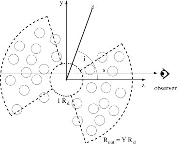
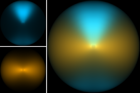
Figure 1: Left: vertical cut through a schematic toroidal cloud distribution, illustrating integration along a particular path $s$ parallel to the $z$-axis. Dust-free regions such as the central cavity of $1\,R_{d}$ diameter do not contribute to the integral. The torus angular edge is soft, i.e. the cloud number falls off from the midplane like a Gaussian. Note that Clumpy does not realize discrete clouds, but rather the properties of a clumpy medium at any continuous location. Right: what an observer on the left might see; two Clumpy thermal emission maps at 9.5 $\mu{\rm m}$ (MIR, top panel, blue colors) and 860 $\mu{\rm m}$ (submillimeter, bottom panel, orange colors), and their composite (large panel), generated by the same cloud distribution. The model has parameters $\hbox{$\sigma$}=43$°, $\hbox{$i$}=75$°, $\hbox{$Y$}=20$, $\hbox{${\cal N}_{0}$}=10$, $\hbox{$q$}=0.08$, and $\hbox{$\tau_{V}$}=70$. The relative contributions of the two maps to the composite image were normalized for clarity.

Figure 1 shows the geometry of ray-tracing through a Clumpy torus model. The plane of the sky is $(x,y)$, with $y$ pointing up and $x$ perpendicular to the page (pointing away from the reader). The AGN-to-observer LOS is $z$. The torus axis is in the $(y,z)$-plane, inclined from the $z$-axis by an angle $i$. At every coordinate $(x,y)$ in the plane of the sky Clumpy computes the monochromatic intensity $I_{\lambda}(x,y)$ along the path $s$ (parallel to the $z$-axis) as the integral over a product of three functions

$$I_{\lambda}(s;x,y)=\int\!\hbox{${d}$}s\,S_{C,\lambda}\,N_{C}(s^{\prime})\,P_{\rm esc}(s^{\prime},s).$$ (5)

$S_{C,\lambda}(s^{\prime})$ is the photon-generating cloud source function at a given point $s^{\prime}$ along the path. $N_{C}(s^{\prime})$ is the local cloud number density from Equation (1) and describes how many clouds are generating the photons. Finally,

$$P_{\rm esc}(s^{\prime},s)=\exp{\left\{-{\cal N}(s^{\prime},s)(1-\exp{(-\tau_{\lambda})})\right\}}$$ (6)

is the probability that a photon generated at $s^{\prime}$ propagates all the way along the rest of the path to the observer without being absorbed again, assuming that the number of clouds is Poisson distributed around the mean (Natta & Panagia, 1984). ${\cal N}(s^{\prime},s)=\int_{s^{\prime}}^{s}N_{C}\,\hbox{${d}$}s$ is the mean number of clouds between point $s^{\prime}$ and the observer, and $\tau_{\lambda}$ the optical depth of a single cloud at wavelength $\lambda$. The convergence of Equation (5) is ensured by Clumpy through Romberg integration.

Ray-tracing for all sky positions $(x,y)$ in the field of view (FOV) generates a 2D image $I_{\lambda}(x,y)$ at wavelength $\lambda$. Figure 1 shows two such maps, and their composite, at 9.5 $\mu{\rm m}$ (blue) and 860 $\mu{\rm m}$ (gold). Correct normalization of these brightness maps, as described in Appendix A of N08b, requires convergence of the area integral $\int\!\hbox{${d}$}x\,\hbox{${d}$}y\,I_{\lambda}(x,y)$; Clumpy handles this via the “Cuhre” integration with globally adaptive subdivision, provided by the Cuba library (Hahn, 2005).

2.3 Wavelength Axis and SEDs

Clumpy computes thermal emission maps $I_{\lambda}(x,y)$ at all specified wavelengths independently. Their area integrals (Section 2.2) and proper normalization produce the SEDs that have been available since 2008 (and are being updated from time to time) for a large number of model parameter combinations.

Table 2: Images Computed at the Following Wavelengths.

No.	Wave	Band		No.	Wave	Band
	($\mu{\rm m}$)				($\mu{\rm m}$)
0	1.2	J		13	12.5	N
1	2.2	K		14	18.5	Q
2	3.5	L		15	31.5	Z
3	4.8	M		16	37.1	Z
4	8.7	N		17	53	A
5	9.3	N		18	89	C
6	9.8	N		19	154	D
7	10.0	N		20	214	E
8	10.3	N		21	350a	10	(857 GHz)b
9	10.6	N		22	460a	19	(652 GHz)b
10	11.3	N		23	690a	18	(434 GHz)b
11	11.6	N		24	945a	17	(317 GHz)b
12	12.0	N

Note. — ^aAt center of bandpass, computed in wavelength space. ^bALMA bandpass central frequency. See Cycle-6 Handbook: https://almascience.nrao.edu/documents-and-tools/cycle6/alma-technical-handbook

For this release of Hypercat we have sampled $N_{\lambda}=25$ wavelengths, listed in Table 2. The wavelengths were chosen strategically based on these criteria: (i) cover all the important bands by available and upcoming instruments, (ii) ensure a spectrally well-sampled 10 $\mu{\rm m}$ silicate feature, (iii) enable interpolation between wavelengths, including in the Raleigh-Jeans tail of the SEDs. However, we needed to limit the number of offered wavelengths to keep the data size of the hypercube manageable. Note that the images are monochromatic, which is justified under the assumption of very narrowband filters commonly used in IR observations of AGNs..

We point out that although Hypercat has a discrete sampling of wavelengths, images at any wavelength within the 1.2–945 $\mu{\rm m}$ range can be computed through interpolation. An approximate SED can be easily extracted, interpolating if necessary between the 25 sampled wavelengths in the hypercube (see User Manual). For studies geared toward SEDs that require a higher spectral resolution, we refer the reader to the established rich grid of model SEDs available on the Clumpy website. These model SEDs have been successfully exploited since their introduction in N08a and N08b, in most cases to fit the observed nuclear but unresolved emission of AGNs (e.g., Asensio Ramos & Ramos Almeida, 2009; Nikutta et al., 2009; Alonso-Herrero et al., 2011; Ramos Almeida et al., 2011; Privon et al., 2012; Ichikawa et al., 2015; Sales et al., 2015; Fan et al., 2016; Fuller et al., 2016; Xie et al., 2016; Audibert et al., 2017; Mateos et al., 2017; Ricci et al., 2017; García-Bernete et al., 2019; González-Martín et al., 2019a, b).

2.4 Simplifications and Caveats

The Clumpy models, as well as the underlying Dusty radiative transfer models, make certain simplifying physical assumptions. The present work does not aim to modify these computations; thus, Hypercat inherits their limitations. Here we note the most important of these.

As published, the Clumpy models represent a single set of dust grain optical properties – a standard ISM mix of cold astrophysical silicates (Ossenkopf et al., 1992) and graphites (Draine, 2003) – and a parameterized power-law grain size distribution following Mathis et al. (1977). The “cold” interstellar silicates from Ossenkopf et al. (1992) are especially successful in fitting the silicate depths observed in AGNs, at both 10 and 18 $\mu{\rm m}$ (Nenkova et al., 2008a; Sirocky et al., 2008; Thompson et al., 2009), but we note that changing the optical and physical properties can result in significantly different SED shapes.

Clumpy models can underpredict the amount of near-IR (NIR) emission in type 1 sources (Mor et al., 2009) because the averaged composite grains have a dust sublimation temperature of around 1500 K, whereas larger and more graphite-rich grains can survive up to $\sim$1800 K, thus producing more NIR emission.

Clumpy models do not produce strong silicate emission features and never show very deep silicate absorption. In the context of AGN tori this is a feature of clumpy torus models. Observations of nuclear emission never detected deep silicate absorption. All sources that do exhibit deep silicate absorption either are ULIRGs (Levenson et al., 2007) or suffer LOS absorption along their (host) galactic plane (Goulding et al., 2012).

Clumpy models are computed with a statistical (Poisson) distribution of dusty clouds around a mean value (the parameter ${\cal N}_{0}$), and the resulting radiative transfer solutions are asymptotic averages over many discrete realizations of such distributions. But Clumpy models are not single-instance discrete realizations, unlike, e.g., Monte Carlo models. The benefit is extremely fast model computation. The drawbacks are that model images appear smooth despite being computed for a clumpy medium and that no stochastic deviations from the mean solution can be studied with such models.

The computation of Clumpy cloud source functions involves an iterative scheme between the clouds being directly heated by the AGN and clouds whose LOS to the AGN is blocked and that are only heated by the radiation bath provided by other clouds in their vicinity. Clumpy executes only the first two steps of this iteration. This approximation is valid for volume filling factors $<0.1$ (Nenkova et al., 2008a), which, depending somewhat also on other parameters, holds for $\hbox{${\cal N}_{0}$}\lesssim 12$.

The largest tori in the images released with Hypercat have a radial extent of $\hbox{$Y$}=20$ dust sublimation radii. If these were used to compare with larger tori in nature, the amount of far-IR (FIR) emission from heated dust might be underestimated. It is important to note that at FIR and submillimeter wavelengths there are often significant contributions from other processes, e.g., star formation and synchrotron radiation. Thus, modeling should include these components explicitly. In this work we concentrate on the possibility of resolved emission at MIR wavelengths, that is, tori with $\hbox{$Y$}\leq 20$ are sufficient.

2.5 Image Size and Sampling

Since the 3D cloud distribution is azimuthally symmetric, the 2D brightness distribution in the $(x,y)$-plane is always symmetric about the $y$-axis (left-right symmetry), regardless of inclination $i$. Clumpy exploits this left-right symmetry when computing a brightness map and only ray-traces one half of the image. If requested, it can mirror the computed image about the $y$-axis and output the full $N_{x}\times N_{y}$ pixel image.

In a full-size (square) image, $N_{x}=N_{y}$ and always odd, to ensure that the nuclear unresolved source is chiefly located at the single central pixel. The central source is unresolved under all circumstances. With $\eta$ the user-requested image resolution in units of pixels per $R_{d}$, a full-size image of radial extent $Y$ (in units of $R_{d}$) has dimensions $N_{x}=N_{y}=2\,Y\eta+1$ pixels. A half-size image has dimensions $N_{x}=Y\eta+1$ and $N_{y}=2\,Y\eta+1$ pixels.

Note that the image size (in pixels) depends on one of the parameters of the model: the torus radial extent $Y$. That is, by default the torus image computed by Clumpy always fills the image frame. This is desirable for modeling work but may not be ideal when simulating observations where the FOV is usually much larger than the small AGN torus on the sky. A constant image size (in pixels) irrespective of $Y$ is also necessary for creating from all single images an $n$-dimensional hypercube. We therefore instructed Clumpy to embed all tori within an image frame of constant FOV, regardless of their size. This common size is the largest sampled $Y$ value in our hypercube, $\hbox{$Y_{\rm max}$}=20$. Clumpy writes the emission maps to FITS files (one file per model parameter combination, one 2D slice per wavelength).

2.6 Projected Cloud Number Maps

While ray-tracing, Clumpy also computes the integrated number of clouds along the LOS. For every path $s$ parallel to the $z$-axis in the FOV (i.e. every pixel) this number is ${\cal N}(s)=\int\!N_{C}\,\hbox{${d}$}s$, with $N_{C}$ from Equation (1). All pixels together make up a map of the projected dust cloud number distribution, $C_{d}(x,y)$. Because of the same argument about azimuthal symmetry made in Section 2.5, $C_{\rm d}$ is always left-right symmetric in the image plane, regardless of inclination $i$.

Unlike the emission maps $I_{\lambda}(x,y)$ the cloud maps $C_{d}$ do not depend on $\lambda$ or $\tau_{V}$. Furthermore, from Eqns. (1) and (3) we see that the cloud distributions at fixed $\left\{\hbox{$\sigma$},\hbox{$i$},\hbox{$Y$},\hbox{$q$}\right\}$ are identical in structure for all ${\cal N}_{0}$ up to a factor: ${\cal N}_{0}$ itself. We can thus store just one cloud map $C_{d}(\hbox{${\cal N}_{0}$}\!\!=\!\!1)$ and later multiply it by the desired ${\cal N}_{0}$ when using the cloud maps. This greatly reduces the storage requirements for all cloud maps.

The integral over all pixels in the cloud map yields the total number of clouds in the torus, $n_{\rm tot}=\int\!C_{d}(x,y)\,\hbox{${d}$}x\,\hbox{${d}$}y$. This number is preserved no matter what viewing angle the torus is inclined at. Note that $n_{\rm tot}$ changes with $q$. From Section 2.4 of N08a, $n_{\rm tot}=(N_{C}/A_{C})\,\hbox{${d}$}V$, where the cloud cross section $A_{C}\simeq R_{C}^{2}$ (and $R_{C}$ is the cloud size). From Equation (1), $N_{C}\propto r^{-q}$. With fixed $R_{d}$, $R_{C}$ and ${\cal N}_{0}$ we then obtain $n_{\rm tot}\propto r^{-q}\,\hbox{${d}$}r$, i.e. when $q$ increases, $n_{\rm tot}$ decreases. Figure 2 shows in the first five panels the projected cloud numbers per pixel (per LOS) for a torus with five values of $q$ between 0 and 2, with other parameters fixed at $\sigma$ = 43°, $Y$ = 20, ${\cal N}_{0}$ = 1, and at a viewing angle $i$ = 90°. The radial cloud distribution is visibly concentrated with growing $q$. At the central pixel, i.e. at zero $x$ and $y$ offsets from the center, ${\cal N}$ = 2 always, because ${\cal N}_{0}$ = 1, i.e. there is on average one cloud along a radial ray in the equatorial plane (and one on the far side of the torus). The right panel shows $n_{\rm tot}$ as a function of $q$ normalized to the maximum value of $n_{\rm tot}$, which occurs at $q$ = 0.

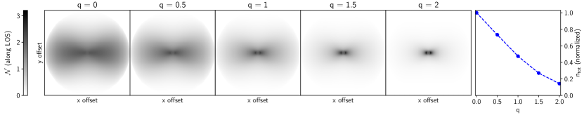
Figure 2: Projected maps of the number of clouds ${\cal N}$ along LOSs for a model with parameters within $q$ = 0–2 as indicated, and other parameters held fixed at $\sigma$ = 43°, $i$ = 90°, $Y$ = 20, and ${\cal N}_{0}$ = 1. All maps are normalized to the same maximum $\hbox{${\cal N}$}_{\rm max}=3.2$ (which occurs at $q$ = 2) and they share the gray scale on the left. The right panel shows the total number of clouds $n_{\rm tot}$ in each map as a function of $q$, normalized to the peak (at $q$ = 0).

These physically motivated maps of dust distributions, when compared to the morphology of the thermal emission emanating from the same torus, can help to understand the conditions that cause the polar elongation of the MIR emission observed in some AGN (or equatorial elongations in other sources, for that matter). The behavior of morphology as a function of position angle (${\rm PA}$), wavelength, and all model parameters can be studied. In Section 3 we analyze the dust and emission morphologies in detail.

2.7 Hypercube Model Files

The parameter sampling of our Clumpy hypercubes is listed in Table 1. The total number of model realizations, without wavelength, is $\prod_{k}\!N_{\theta_{k}}=336,\!000$. The images were computed for $N_{\lambda}=25$ wavelengths, listed in Table 2 (see also Section 2.3); thus, 8.4 million images were computed overall, in addition to 4000 individual dust maps. Computation of the Clumpy brightness maps and dust cloud maps that make up this first release of the hypercube consumed a total of 3.2 yr on mid-tier CPUs.

We deliver all computed brightness maps stored as a 9D hypercube within convenient hdf5 files, in the imgdata group. The same files also contain a 6D hypercube of all projected dust maps (clddata group). See Table 3 and Appendix B for details about the hdf5 files and their internal organization.

Table 3: List of hdf5 Files Containing Clumpy Brightness Maps and Projected Dust Maps.

File Name	Size (GB)		Nwave	Wavelengthsa
	Compressedb	Rawc		($\mu{\rm m}$)
hypercat_20200830_all.hdf5	27100	91300	25	all of the below
hypercat_20200830_nir.hdf5	4400	14600	4	1.2, 2.2, 3.5, 4.8
hypercat_20200830_mir.hdf5	12000	40200	11	8.7, 9.3, 9.8, 10, 10.3, 10.6, 11.3, 11.6, 12, 12.5, 18.5
hypercat_20200830_fir.hdf5	6500	21900	6	31.5, 37.1, 53, 89, 154, 214
hypercat_20200830_submm.hdf5	4200	14600	4	350, 460, 690, 945

Note. — ^aNote that Hypercat can interpolate between the wavelengths. ^bTo be downloaded. ^cUncompressed on disk. Files available at https://www.clumpy.org/images/

3 Morphologies of Thermal Emission and Projected Cloud Number Maps

The emergence of instruments powerful enough to resolve the dusty torus in nearby AGNs (e.g., ALMA, 30 m class telescopes) allows us not only to separate the flux contributions of the nucleus and host galaxy but also to quantify the morphology of the observed nuclear brightness distribution. Resolved VLTI observations (e.g., Hönig et al., 2012, 2013; Tristram et al., 2014; López-Gonzaga et al., 2016) show that in several nearby AGNs the MIR emission is elongated in polar directions, with the polar axis usually defined by other means, e.g., the orientation of ionization cones, a nuclear jet, or the perpendicular orientation of a maser disk. In these sources most of the MIR emission appears to be emanating from regions high above the equatorial plane of the “torus,” i.e. not from where most of the dust is thought to reside according to AGN unification.

Whatever the mechanism for producing an elongated morphology, it must reconcile the 2D brightness map with the 3D dust distribution consistently. NIR and MIR imaging with extremely large single-dish telescopes will resolve the morphology unambiguously, and free of model assumptions. Phenomenological modeling of the brightness distribution can no longer serve as a surrogate.

In this section we investigate the morphologies of Clumpy brightness maps in several wavelength regimes and of their underlying dust distribution maps. We introduce and measure various morphological quantities, e.g., centroid location, half-light radii (1D), radii of gyration (2D), elongation (aspect ratio) of the morphology, position angle, asymmetry (skewness), and compactness (peakedness). We first investigate the morphological changes to brightness maps as a function of model parameters, with a focus on identifying the part of parameter space that allows for polar elongation of brightness distributions similar to those reported in the literature. We then compare these brightness maps to their corresponding dust maps, inferring as a function of model parameters the localized correspondence (or lack of it) of dust distributions and the emission morphologies generated by them. In Paper II we will then simulate observations with extremely large telescopes and compare to observational results obtained for NGC 1068.

3.1 Image Moments and Moment Invariants

Table 4: Useful Morphological Measurements with Moments.

Measure / Method
Image mass (sum), or “flux”
$M_{00}$ or $\mu_{00}$ (identical)
Image centroid location
$\bar{x}=M_{10}/M_{00}$,  $\bar{y}=M_{01}/M_{00}$
Radius of gyration about axis
$R_{g}^{x}=\sqrt{\mu_{20}/\mu_{00}}$,  $R_{g}^{y}=\sqrt{\mu_{02}/\mu_{00}}$
Elongation in the $y$-direction
$e=R_{g}^{y}\,/\,R_{g}^{x}$
Image covariance matrix
$\mathrm{Cov}[I(x,y)]=\begin{bmatrix}\mu^{\prime}_{20}&\mu^{\prime}_{11}\\ \mu^{\prime}_{11}&\mu^{\prime}_{02}\end{bmatrix}$
${\rm PA}$ of main component
$\dfrac{1}{2}\arctan\left\{2\,\mu^{\prime}_{11}\Big{/}\left(\mu^{\prime}_{20}-\mu^{\prime}_{02}\right)\right\}\ \rm(radian)$
Skewness
$S_{x}=\mu_{03}\Big{/}\sqrt{\mu_{02}^{3}}$,  $S_{y}=\mu_{30}\Big{/}\sqrt{\mu_{20}^{3}}$

Note. — $M_{\rm pq}$ raw moment (Equation C1), $\mu_{\rm pq}$ central moment (Equation C3), $\mu^{\prime}_{\rm pq}=\mu_{\rm pq}/\mu_{00}$ second-order central moment (see Appendix C.2), $I(x,y)$ image.

We quantify the morphologies in terms of their image moments and quantities computed from moments, and we compare them to some traditional morphological quantifiers. The so-called central moments are

$$\mu_{\rm pq}=\sum_{x}\sum_{y}I(x,y)\,(x-\bar{x})^{p}\,(y-\bar{y})^{q},\quad p,q\in\mathbb{N},$$ (7)

where $\bar{x}$ and $\bar{y}$ are the image centroid coordinates in pixels. By construction central moments are invariant under translation operations. Combinations of moments can be defined that are invariant under translation, scaling, rotation, or any combination of these operations. We refer to Appendix C for a technical discussion. Functions of image moments can be used to compute various quantities that characterize morphology. Table 4 lists the ones that we make use of in this paper.

3.2 Size, Elongation, and Image Compactness

We wish to quantify the spatial extension of emission morphologies as a function of model parameters. Various measures have been proposed in the literature, e.g., the half-light radius, the FWHM of a fitted 2D Gaussian, or the Petrosian radius (Petrosian, 1976; Graham et al., 2005). We show that a quantity based on image moments, the radius of gyration, is ideally suited to measure morphology size. We also introduce the Gini index as a simple way to quantify image compactness. For the remainder of the paper we can assume that there is only one extended source present in the image – the model torus.

3.2.1 Half-light Radius

A commonly used size estimate of an emission region is the half-light radius $R_{\rm HL}$ of a circular aperture that contains half of the total flux in the image (see Appendix C.5). The aperture is usually anchored on the origin of the coordinate frame. However, the half-light radius is sensitive to where the aperture is centered in the general case that the brightness distribution is not uniform. Figure 3 shows a 10.0 $\mu{\rm m}$ image of a Clumpy torus model at several viewing angles $i$, as indicated. All other model parameters are fixed.

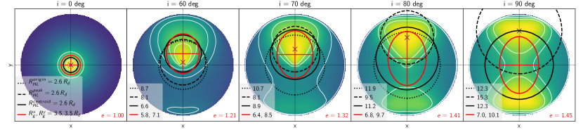
Figure 3: Morphological size measurements on 10 $\mu{\rm m}$ images of a model at several inclination angles $i$ (columns). Inclinations between 0° and 60° are similar in appearance and for clarity not shown. ${\cal N}_{0}$ is set at 9, and all other parameters are fixed at the best values from SED fitting of NGC 1068 given in Lopez-Rodriguez et al. (2018): $\sigma$= 45°, $Y$= 18, $q$= 0.08, $\tau_{V}$= 70, $i$= 75°. These values are also used throughout Paper II. The $Y=18~{}R_{d}$ torus is embedded in a $2\times 20~{}R_{d}$ FOV frame. Images are log-stretched and normalized independently. White contour lines computed on the linearly scaled images are shown at 5%, 10%, 30%, 50% of the peak pixel, which is marked with a black cross. Red horizontal and vertical lines show the radii of gyration $R_{g}^{x}$, $R_{g}^{y}$ about the $x$ and $y$-axes; they form the semimajor axes of the red ellipse encompassing them, centered on the image centroid $(\bar{x},\bar{y})$. For pole-on view ($i$ $=0$°) we set the peak location to the image origin. Three black circles show apertures with half-light radii centered on the origin (dotted), emission peak (dashed), and the centroid (solid). All three contain half the light in an image. In pole-on view all three circles are centered on the origin and thus of equal radius. In edge-on view it depends on the parameter combination whether the peak pixel will be at the origin or higher above the equatorial plane (as is the case here, with two symmetric peak pixels). The legend lists the half-light and gyration radii in units of $R_{d}$. The elongation $e=R_{g}^{y}/R_{g}^{x}$ is printed in the lower right corner.

Three circular apertures are shown, centered at different loci, and each contains half the light of the image. Because the brightness distribution is not uniform across the image, these half-light radii differ in size.

In pole-on view ($i$ = 0°) all half-light radii are identical, since all apertures are centered on the origin. Note that in pole-on view the “brightest pixel” is ill-defined; it is in fact a ring around the image origin. We thus set the aperture center to the center pixel. In edge-on views the three circles are only identical if the brightest pixel happens to be at the image center. This is the case if the central LOS is optically thin or mildly obscured. If the absorption along the central LOS increases, through either a higher ${\cal N}_{0}$ or a higher $\tau_{V}$, or through a change in wavelength, the emission peak occurs spatially much higher above the equatorial plane, and thus the half-light aperture constructed around the peak pixel is very different from the centroid- and origin-based ones.

Unresolved measurements of the total flux are of course not affected by the choice of the aperture center, since all flux is within the PSF. Interferometers without phase closure, such as VLTI with two telescopes, can resolve the nuclear emission in some nearby AGNs, but the emission cannot be localized within the FOV since absolute astrometry cannot be achieved. However, interferometers with phase closure (e.g., VLTI with MATISSE or GRAVITY, ALMA) and, of course, very large single-aperture telescopes (e.g., GMT, TMT, ELT) do attain absolute astrometry; thus, the locus at which the half-light radius aperture is anchored can be important. We note though that for extragalactic observations of (marginally) resolved nuclear cores, precise image registration is critical (Prieto et al., 2014).

In the edge-on scenario shown in Figure 3, the offset between the image origin and the brightest pixel is about 12.3 $R_{d}$. The physical size depends on luminosity; for NGC 1068 it is quite uncertain. Our own fitting (in Paper II) of the $K$-band image by Gravity Collaboration et al. (2020; hereafter G20) yields ${L_{\rm bol}=1.56\times 10^{44}\,\rm erg\,s^{-1}}$ or ${L_{\rm bol}=2.62\times 10^{44}\,\rm erg\,s^{-1}}$ depending on the model; García-Burillo et al. (2014) find ${L_{\rm bol}=4.2\times 10^{44}\,\rm erg\,s^{-1}}$ from SED fitting; Lopez-Rodriguez et al. (2018) report ${L_{\rm bol}=5.02\times 10^{44}\,\rm erg\,s^{-1}}$ when including FIR data (see also Paper II); Alonso-Herrero et al. (2011) adopted ${L_{\rm bol}=1\times 10^{45}\,\rm erg\,s^{-1}}$; Raban et al. (2009) give ${L_{\rm bol}=1.5\times 10^{45}\,\rm erg\,s^{-1}}$; Burtscher et al. (2013) list ${L_{\rm bol}=1.58\times 10^{45}\,\rm erg\,s^{-1}}$.

This range of luminosities translates to sizes between 1.9 and 6.2 pc for the 12.3 $R_{d}$ offset and, with a distance of 14.4 Mpc to NGC 1068, between 28 and 89 mas angular extent on the sky. The larger values are well above the diffraction limit of 30–40 m class telescopes. Figure 4 shows the angular size of 12.3 $R_{d}$ on the sky, as a function of AGN bolometric luminosity (which sets the distance of the dust sublimation radius) and of source distance, together with the diffraction limit of telescopes with 6.5–100 m diameters $D$ ($\theta=1.22\,\lambda/D$) at 10 $\mu{\rm m}$. The bolometric luminosities for NGC 1068 listed above are marked in the figure. The effect described above is potentially resolvable with 30 and 40-m class telescopes, if good astrometry can be achieved. Smaller telescopes would struggle, unless a source were much brighter than NGC 1068, and/or closer than it (but such sources do not exist). The same is true if the bolometric luminosity of the source is on the lower end of the range. Other nearby AGNs at similar distances have larger tori, which makes the situation easier (e.g., Alonso-Herrero et al., 2018, 2019; Combes et al., 2019).

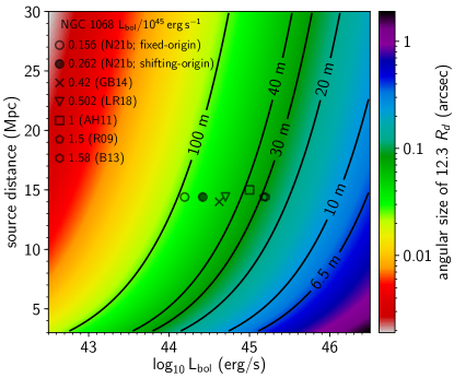
Figure 4: Angular size on the sky (in arcsec) of a structure 12.3 $R_{d}$ large (corresponding to the $y$ offset between image origin and brightest pixel in the rightmost panel of Figure 3), as a function of AGN bolometric luminosity and source distance, shown as a logarithmic color map. Labeled contour lines trace the diffraction limit at $10\!~{}\hbox{$\mu{\rm m}$}$ of telescopes between 6.5 and 100 m diameter. Sources with luminosity and distance below a certain contour produce structures that can be potentially resolved by the corresponding telescope. The symbols indicate various bolometric luminosities reported for NGC 1068 in the literature, which vary by a factor of several: this work (N21b, fitting directly the $K$-band image from G20, two models, see Paper II), García-Burillo et al. (2014; GB14), Lopez-Rodriguez et al. (2018; LR18), Alonso-Herrero et al. (2011; AH11), Raban et al. (2009; R09), and Burtscher et al. (2013; B13). Most references adopted $D=14.4$ Mpc as the source distance, except GB14 (14 Mpc) and AH11 (15 Mpc).

Another drawback of half-light radii is that they cannot measure morphology sizes independently for orthogonal directions on the sky. In the following subsection we remedy this by introducing radii of gyration.

3.2.2 Radii of Gyration

A very robust way to measure image extension is via radii of gyration about the $x$ and $y$-axes

$$R_{g}^{x}=\sqrt{\mu_{20}/\mu_{00}},\qquad R_{g}^{y}=\sqrt{\mu_{02}/\mu_{00}}.$$ (8)

The gyration radius about an axis is the distance to a line parallel to the axis, at which all the “mass” (i.e. all the pixel values) could be concentrated without changing the second moment about that axis. Like other quantities computed from image moments, the concept of gyration radius is borrowed from mechanics. Figure 3 shows the gyration radii $R_{g}^{x}$, $R_{g}^{y}$ as the semimajor axes of a red ellipse, plotted over the brightness distributions produced by a Clumpy model. The ellipse is centered on the image centroid $(\bar{x},\bar{y})$.

When estimating morphology sizes, the radii of gyration have several benefits over other measures, such as the half-light radius. One is that they give realistic estimates of both the $x$ and $y$ extensions independently. This allows us then to compute the elongation or aspect ratio of the brightness distribution, which we will explore in the next subsection. Further, in all but the $i$ = 90° case, where the image may show two bright centers of emission offset in the $\pm y$-direction, the ellipse made of gyration radii and anchored on the image centroid follows the bulk of the emission more faithfully than circular apertures pinned to the telescope pointing (usually the suspected locus of the AGN).

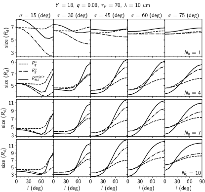
Figure 5: Morphological size measurements of brightness maps at 10 $\mu{\rm m}$. Torus parameters $\hbox{$Y$}=18$, $\hbox{$q$}=0.08$, and $\hbox{$\tau_{V}$}=70$ are fixed, while $\sigma$, ${\cal N}_{0}$, and $i$ vary as indicated. Vertical scale is the same only per row. Solid lines show the half-light radius $R_{\rm HL}^{\rm origin}$ of an aperture centered on the image origin. Dashed lines show the radius of gyration in $x$-direction, $R_{g}^{x}$, while dashed-dotted lines show $R_{g}^{y}$, the radius of gyration in $y$-direction.

Figure 5 shows how the radii of gyration, $R_{g}^{x}$ and $R_{g}^{y}$, and the half-light radius, $R_{\rm HL}^{\rm origin}$, depend on (a subset of) the torus model parameters. The analysis was performed on the “infinite” resolution model images (at 10 $\mu{\rm m}$) to illustrate direct physical effects of parameter changes on image morphology. Plotted as a function of viewing angle, the half-light radius varies most extremely among the three shown size measurements. In most cases (${\cal N}_{0}$ = 1 being the exception) $R_{\rm HL}^{\rm origin}$ is the lowest at pole-on viewing angles and the largest at edge-on orientations. That is, the half-light radius likely underestimates/overestimates the characteristic sizes at pole-on/edge-on viewings. The radii of gyration respond more gently to changes in model parameters. Naturally, $R_{g}^{y}$ varies more strongly than $R_{g}^{x}$ with viewing angle $i$ and torus angular size $\sigma$, as these two quantities have the largest influence on the size of the image morphology in the $y$-direction. ${\cal N}_{0}$ (and $\tau_{V}$, which is not varied in this figure) provides the overall magnitude of the measured size.

In the case of very high $\sigma$ and ${\cal N}_{0}$, i.e. an optically and geometrically thick dust “cocoon” scenario (lower right panel in Figure 5), both radii of gyration show very little variation with viewing angle, while the half-light radius still changes strongly between pole-on and edge-on viewing.

3.2.3 Aspect Ratio / Elongation

Because the radii of gyration about the $y$ and $x$-axes measure morphological size independently in both directions, their aspect ratio determines the elongation of the morphology

$$e=R_{g}^{y}\,/\,R_{g}^{x}.$$ (9)

In our model images the position angle is always ${\rm PA}=0$°, i.e., $R_{g}^{y}$ corresponds to the polar direction and $R_{g}^{x}$ to the equatorial direction.

Using this technique, we now want to measure the elongation of torus images produced by Clumpy while varying the model parameters. Figure 6 shows the elongation measured from images for a number of parameter variations, at five wavelengths between NIR and submillimeter, and for two different radial cloud distribution power laws (flat, with $q$ = 0.08 on the left, and steep, with $q$ = 2 on the right). The measurements are considering all pixels in an image unless stated otherwise.

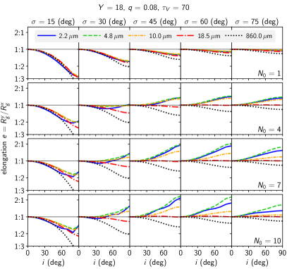
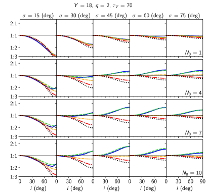
Figure 6: Elongation $e=R_{g}^{y}/R_{g}^{x}$ of image morphology. The vertical axis is logarithmic, which is the natural measure for ratios, with some integer ratios marked. A thin horizontal solid line in every panel marks the 1:1 aspect ratio, i.e. $e=1$. Values $e>1$ show elongation in the $y$-direction (polar extension), and $e<1$ in the $x$-direction (equatorial extension). The five line styles and colors encode five different wavelengths from NIR to submillimeter (see legend). Torus parameters $\hbox{$Y$}=18$ and $\hbox{$\tau_{V}$}=70$ are fixed, while $\sigma$, ${\cal N}_{0}$, and $i$ vary as indicated. The radial steepness of the cloud distribution law is flat in the left panels ($q$ = 0.08) and steep in the right panels ($q$ = 2). For flat distributions polar elongations can be achieved at NIR and MIR wavelengths. At steep distributions no elongation in the MIR is possible.

Several characteristics are immediately apparent. All curves begin at precisely $e=1.0$ for $i$ = 0°. This is so because for pole-on LOSs the torus appears perfectly circular. Conversely, the largest and smallest aspect ratios are realized at or very close to edge-on views ($i$ = 90°).

Another observation is that it is impossible to achieve any level of polar elongation at small values of $\sigma$ or at the smallest values of ${\cal N}_{0}$. A torus whose distribution of dust clouds is disk-like and concentrated in the equatorial plane will always appear elongated in the equatorial direction, i.e. perpendicular to the torus axis. At small $q$ values no net polar elongation can be achieved at FIR and submillimeter wavelengths with any combination of parameters. This is because the total optical depth through the torus is small at these wavelengths, so the emission morphology mostly follows the dust distribution, i.e. it resembles the torus in appearance (see Section 3.4 for more details). For steep distributions ($q$ = 2) no polar elongation is possible even in the $N$ band (MIR).

Significant polar elongation in emission can be easily achieved at intermediate to large viewing angles, moderate to large ${\cal N}_{0}$, and wavelengths between the $K$ and $N$ bands (for small $q$), with the highest aspect ratios observed in the $M$ band, around 4.8 $\mu{\rm m}$. The highest elongations require $\hbox{$\sigma$}\approx 45\arcdeg-60\arcdeg$, and $\hbox{$i$}\approx 90$°.

Figure 7 shows the aspect ratio for many parameter variations, but as heat maps. Parameters $i$ = 75°, $q$ = 0.08, and $Y$ = 18 are held fixed, and the other parameters vary as indicated.

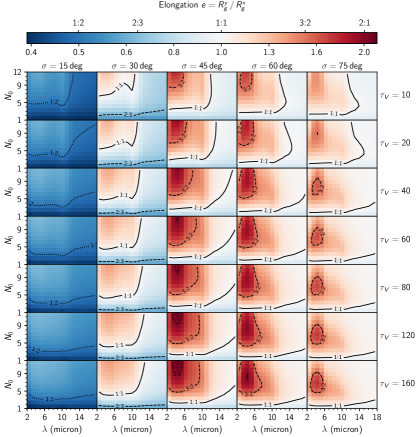
Figure 7: Image elongation $e$ as a function of model parameters, shown as heat maps. Red colors show elongation in the $y$-direction (polar), blue colors in the $x$-direction (equatorial). Some best-fit parameter values from SED fitting of NGC 1068 are held fixed, i.e., $i$ = 75°, $q$ = 0.08, $Y$ = 18, while all other parameters vary as indicated. All panels are normalized to the same range and are logarithmically stretched separately for values smaller/greater than 1.0 (see color bar). Contour lines show aspect ratios 1:1 (solid), 2:3 and 3:2 (dashed), and 2:1 and 1:2 (dotted), also marked on the color bar (upper tickmarks).

Regions of significant polar elongation are clearly visible as areas of deep red color in the panels. The highest realized polar elongation for the NGC 1068 case shown in the figure is $e=2.13$ and is realized at $(\hbox{$\sigma$},\hbox{${\cal N}_{0}$},\hbox{$\tau_{V}$},\lambda)=(45\arcdeg,12,160,\hbox{$\sim$}4.0~{}\hbox{$\mu{\rm m}$})$. The smallest ratio in the figure, i.e., the highest in equatorial direction, is $e=0.39$. More extreme ratios require more edge-on viewing angles.

MIR observations with long-baseline interferometry on VLTI (Burtscher et al., 2013; and references therein) measured polar elongations of nuclear dust emission for a number of sources: $\sim$2 (for Circinus), 1.3 for NGC 3783, 1.5 for NGC 424, and 1.3 for NGC 1068, the example object of our study. These elongations are easily achievable with Clumpy torus images. For instance, with $i$ held at 75°, model image elongation ranges up to 1.5 at 10 µm; it can reach well above 2 at higher inclinations. Thus, Clumpy torus models naturally can reproduce the polar elongation of the spatial flux distribution in the $N$ band up to several parsecs away from the AGN.

Interferometric observations that include shorter baselines are sensitive to the brightness distribution on larger spatial scales, i.e., farther away from the nucleus. López-Gonzaga et al. (2016) reported on such observations with VLTI, adding the AT telescopes, and found even larger polar elongations on such scales for several sources: 1.9 for NGC 424 (and for Circinus), 2.3 for NGC 1068, 2.5 for NGC 5506, and 3.1 for NGC 3783. In addition, Leftley et al. (2018) find $e=2.9$ for ESO323-G77. Note that for Circinus and NGC 1068 these values are lower limits, as the extended emission is over-resolved interferometrically and continues in single-dish observations. NGC 3783 and ESO323-G77 are type 1 AGNs, meaning that our viewing lines to them are most likely not too highly inclined. As we have seen in figures 6 and 7, high inclinations are necessary to produce significant polar elongation of the MIR morphology. In these type 1 sources a two-component model is therefore almost certainly preferred. For the above measurements, the authors estimated polar elongation by fitting 2D Gaussians, but the FWHM of a Gaussian is equivalent to the radii of gyration we use here (although our moment-based method works for any morphology).

Achieving elongations of 2.5 or even 3 with single-component models (i.e. a torus) may be challenging, or impossible in type 1 orientations. Two-component models, such as a disk and a dusty outflow, provide the necessary morphology by design, but at the cost of higher model complexity. The measured elongation, however, always depends on the pixels considered. Just as in the case of VLTI measurements with UT baselines only, versus UT+AT baselines, the sensitivity to larger spatial scales changes the derived elongations. Similarly, an instrumental flux sensitivity limit will affect which pixels will in fact be considered when estimating morphological parameters.

Figure 8 illustrates this with two Clumpy torus models, one with parameters from SED fitting in LR18, and a version of it with parameters somewhat modified to increase elongation. The elongation measured as a function of wavelength and sensitivity level (i.e. which contour is the limiting isophote) varies strongly. In the LR18 model, at 10 $\mu{\rm m}$, considering the entire image yields $e=1.2$, but it reaches 1.43 for the 7% contour. This SED-derived model is elongated enough to explain the value of $e=1.3$ measured by VLTI for NGC 1068 (Burtscher et al., 2013) with long baselines alone. It is not elongated enough to explain $e=2.3$ derived for VLTI observations López-Gonzaga et al. (2016) performed on larger spatial scales.

Modifying some of the model parameters (e.g., higher $\sigma$, $i$, ${\cal N}_{0}$, $\tau_{V}$) can produce models with larger polar elongations. In Figure 8 the bottom row shows one such model; it produces $e=1.41$ at 10 $\mu{\rm m}$ if the entire image is considered. However, the same model shows much higher elongations at other sensitivity levels, e.g., $e=3.22$ at the 0.5 level of the peak.

To match observations, not only the elongation but also the angular size of the morphology must be considered. In this release of Hypercat our sampling of the torus size (the $Y$ parameter) tops out at $Y$ = 20. With larger values and sufficiently high luminosity it is possible that such elongations could be maintained on larger physical scales.

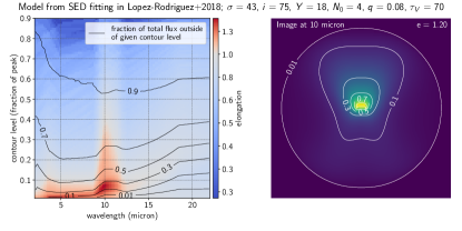
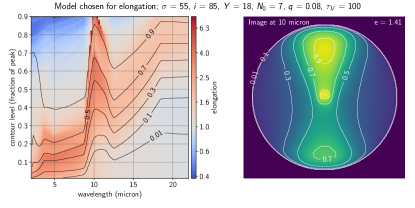
Figure 8: The effect of sensitivity on measured elongation. Two models are shown. Top: with parameters derived from SED fitting in LR18. Bottom: similar to the top model, but with parameters modified for elongation. Each left panel shows as a color map the elongation $e=R_{g}^{y}/R_{g}^{y}$ of all pixels contained within a given contour level (given as a fraction of the peak) on the $y$-axis and of wavelength on the $x$-axis. For instance, in the bottom model at 10 $\mu{\rm m}$ and 0.5 contour the elongation reaches 3.22, while the entire image (i.e. contour level 0) has only $e=1.41$. The overplotted black lines show the fraction of total flux that is outside of a given contour, i.e. is being missed at a given sensitivity level. For example, in the bottom model at 10 $\mu{\rm m}$ and 0.5 isophote a fraction of 0.43 of the total flux is outside that isophote. The right panels show the image at 10 $\mu{\rm m}$ from each model, with contour levels shown as white lines at 0.01, 0.1, 0.3, 0.5, 0.7, 0.9 of the peak. These contours correspond to the $y$-axis in the left panel. The elongation $e$ printed in the upper right corners is for the entire image (contour level 0).

Somewhat similar to the question of brightness level sensitivity, a potential pitfall in resolved observations is that the measured elongation of a brightness distribution depends on the FOV. This effect may even invert the axis of elongation, depending on the FOV. Figure 9 demonstrates this with a 4.8 $\mu{\rm m}$ image of a $Y$ = 20 torus model, looked at with progressively larger FOVs. From small to large FOV, the measured elongation $e=R_{g}^{y}/R_{g}^{x}$ turns from slightly elongated in the equatorial direction to very elongated along the polar axis, as indicated in the panels.

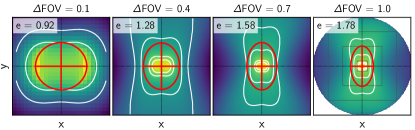
Figure 9: Image elongation as a function of FOV. The same model is shown in all panels, with parameters $\sigma$ = 45°, $i$ = 90°, $Y$ = 20, ${\cal N}_{0}$ = 7, $q$ = 0, $\tau_{V}$ = 40, $\lambda$ = 4.8 $\mu{\rm m}$. The rightmost panel shows the full image, while the three left panels show fractional FOVs ($\Delta$FOV = 0.1, 0.4, 0.7 of the full FOV). Light-gray squares in the right panel indicate the other FOVs. The intensity maps are log-stretched, while contour lines (white) are computed on the linear image at 5%, 10%, 30%, and 50% percent of the peak pixel. Red ellipses show the morphological sizes measured by radii of gyration. From small to large FOV, the measured elongation $e=R_{g}^{y}/R_{g}^{x}$ turns from slightly elongated in the $x$-direction (equatorial) to very elongated in the $y$-direction (polar), as indicated in the panels.

3.2.4 Gini Coefficient as Indicator of Image Compactness

The Gini coefficient / index (Gini, 1921) was originally developed in the field of economics to characterize the relative inequality of income distributions. It is applicable generally, though, and is a useful measure of image compactness in our case. Applied to the distribution of pixel values, it measures the relative deviation of the distribution from uniformity. In the discrete case, the Gini coefficient of an array $I$ is

$$G=\frac{\sum_{i}(2i-n-1)\cdot I_{i}}{n\sum_{i}I_{i}}$$ (10)

where the $n$ values $I_{i}$ of the array are sorted in ascending order, and $i$ are the corresponding (one-based) indices of the sorted array. In our case of a 2D image, $I(x,y)$ can be simply flattened prior to computing $G$. The Gini index is independent of the absolute magnitude of the pixel values; only their relative distribution matters. If all values are identical, $G=0$. If the distribution is randomly uniform, $G=1/3$. In the most unequal distribution, a delta function (e.g., when exactly 1 pixel has nonzero value), $G=1$.

Figure 10 shows $G$ as a function of several parameters that vary as indicated. $Y=18$, $q=0$ and $\hbox{$i$}=90$ $\rm deg$ are fixed.

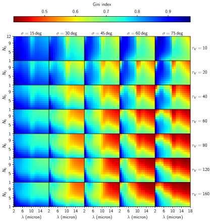
Figure 10: Image compactness, measured as the Gini index, for a number of model parameters that vary as noted. $Y=18$, $q=0$ and $\hbox{$i$}=90$° are fixed. Blue colors are compact morphologies, red colors are extended images. The maximal range of the Gini index is from 0 (all pixels equal) to 1 (a single pixel is nonzero). The size enhancement around 10.0 $\mu{\rm m}$ due to the increased dust absorption coefficient is clearly visible.

Values close to unity (dark blue colors) are the most compact morphologies, where all flux is concentrated within a small fraction of all pixels. Lower values (red colors) represent broader distributions. For the $Y=18$ torus embedded in a $(2\,Y_{\rm max})^{2}=40\times 40$ FOV, the smallest achievable $G$ value is $\sim$0.36. This would be the case if all the pixels within a $Y=18$ circle had the same value while pixels outside that circle were zero (we are ignoring the central dust-free cavity for the sake of simplicity). The smallest $G$ in figure 10 is 0.40, i.e. there are models whose appearance approaches that of a uniformly bright disk. Not surprisingly, the corresponding model parameters represent the thickest and most dense torus of all shown in the figure, namely $(\hbox{$\sigma$},\hbox{${\cal N}_{0}$},\hbox{$\tau_{V}$},\lambda)=(75~{}\rm deg,12,160,18~{}\hbox{$\mu{\rm m}$})$. The elongation of this morphology is $e=R_{g}^{y}/R_{g}^{x}=1$. On the other hand, the most compact emission morphology is realized with the most shallow torus, smallest number of clouds, lowest optical depth, and shortest wavelength $(\hbox{$\sigma$},\hbox{${\cal N}_{0}$},\hbox{$\tau_{V}$},\lambda)=(15\,\rm deg,1,10,2\,\hbox{$\mu{\rm m}$})$. This smallest model has $G=0.97$ and elongation $e=0.31$. Figure 18 in Appendix C.6 shows both extremes.

In general, compact images are achieved at small ${\cal N}_{0}$, small $\lambda$, and preferentially at small optical depths. For large optical depths, only the very smallest ${\cal N}_{0}$ and shortest wavelengths can produce compact emission sizes, i.e. when only the hottest dust close to the center is visible. In Figure 10, at small to moderate $\tau_{V}$ and moderate to high ${\cal N}_{0}$ a size enhancement is clearly visible around 10 $\mu{\rm m}$. This is because the dust cross section peaks locally around 10 $\mu{\rm m}$, increasing the optical depth, thus intercepting more photons, also at greater distances, before they can escape the torus. At wavelengths slightly away from the peak of the dust cross-section curve the photon escape probability is significantly higher (see Figure 2 in Nenkova et al., 2008b).

3.3 Image Asymmetry

The interplay between torus angular width $\sigma$, viewing angle $i$, and total optical depth along an LOS can shift the region that emits light (as viewed by an observer) up or down from the image center. This asymmetry in the distribution of emission can be quantified in several ways.

3.3.1 Thermal Emission Distribution

Probably the simplest measure of asymmetry with respect to the $x$-axis is the fraction of total light contained in the upper image half. This fraction is by design 0.5 in pole-on and edge-in views, but for other inclination angles will depend on some of the model parameters. Figure 11 shows this for a number of typical model parameter combinations and four wavelengths between 2.2 and 18.5 $\mu{\rm m}$.

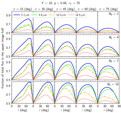
Figure 11: Fraction of total light contained in the upper image half, as a function of model parameters. Torus parameters $\hbox{$Y$}=18$, $\hbox{$q$}=0.08$, and $\hbox{$\tau_{V}$}=70$ are fixed, while $\sigma$, ${\cal N}_{0}$, and $i$ vary as indicated. The four line styles and colors show four different wavelengths (see legend).

The asymmetry is largest at short wavelengths ($K$ band), as this is mostly scattered light from the far inner side of the torus. Longer wavelengths can penetrate deeper into the torus in all directions, diminishing the asymmetry in light distribution among the upper and lower image halves. The fraction as a function of viewing angle always has a clear peak, and for all $\hbox{$\sigma$}>45$° and short wavelengths it is approximately symmetric around $\hbox{$i$}\approx 45$°. At smaller $\sigma$ or longer wavelengths the peak occurs roughly at $90\arcdeg-\hbox{$\sigma$}$, i.e. at the torus half-opening angle. Increasing optical depth via higher ${\cal N}_{0}$ increases the overall scale of the emission asymmetry.

The fraction of emission from regions above the nucleus can easily reach 90% or more at 2.2 and 4.8 $\mu{\rm m}$, and over 80% at 10 $\mu{\rm m}$. At 18.5 $\mu{\rm m}$ the asymmetry tops out at $\sim$70%, but it is significantly less in most cases.

In Section 3.4 we will demonstrate that although the distribution of the thermal emission can be highly asymmetric in many configurations, it does not necessarily correlate with the physical distribution of the dust in the torus, whose bulk is still in the equatorial plane.

3.3.2 Centroid Offset

A different method to quantify the asymmetry in emission distribution is by measuring the $y$ position of the brightness centroid, $\bar{y}$. Figure 12 shows this in a similar fashion to Figure 11, but the $y$-axis in each panel is the vertical offset of the light centroid from $y$=0 in units of dust sublimation radius $R_{d}$.

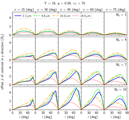
Figure 12: Vertical offset of the image centroid, $\bar{y}$, in units of dust sublimation radius $R_{d}$. Torus parameters $\hbox{$Y$}=18$, $\hbox{$q$}=0.08$, and $\hbox{$\tau_{V}$}=70$ are fixed, while $\sigma$, ${\cal N}_{0}$, and $i$ vary as indicated. The four line styles and colors show four different wavelengths (see legend).

In $K$ through $M$ bands these curves always peak close to edge-on viewings, but not quite at $\hbox{$i$}=90$° of course, as this is a symmetric morphology. The N band behaves similarly, albeit transitioning to the longer-wavelength case, where the $Q$ band curve shows a much more symmetric shape around $\hbox{$i$}\approx 45$°. The 2.2 and 4.8 $\mu{\rm m}$ images show the largest centroid shifts (of very similar magnitude) and can be quite substantial, up to 5 $R_{d}$, i.e., almost 30% of the torus overall radius in this $\hbox{$Y$}=18~{}R_{d}$ case. The centroid offsets at 10.0 $\mu{\rm m}$ are a bit smaller, and at 18.5 $\mu{\rm m}$ they are the smallest of all. Again, this is due to long-wavelength photons traveling more freely in all directions and into the torus, thus reducing the asymmetry. The dependency of $\bar{y}$ on ${\cal N}_{0}$ is stronger than that of the emission fraction in the upper image half discussed in the previous subsection.

3.3.3 Skewness

Using the image moments developed earlier, the asymmetry of emission distribution can be quantified by measuring skewness. The skewness of a distribution of pixel values, projected onto the axes, is a third-order moments function:

$$S_{x}=\mu_{03}/\sqrt{\mu_{02}^{3}},\qquad S_{y}=\mu_{30}/\sqrt{\mu_{20}^{3}}.$$ (11)

It measures the deviation from a symmetric distribution in the given direction. Since Clumpy images are always symmetric about the $y$-axis, the skewness $S_{y}$ is always zero. We thus only consider $S_{x}$, the image skewness about the $x$-axis (i.e. in the $y$-direction). Negative values of skewness indicate asymmetry toward the positive direction of an axis. Note that a zero-valued skewness does not guarantee symmetry, but a symmetric distribution will always have skewness zero.

Figure 13 plots $S_{x}$ for Clumpy model images at three wavelengths and as a function of several torus model parameters that vary as indicated. For all but the very smallest value of ${\cal N}_{0}$, the skewness curves appear very similar in shape for a given $\sigma$ and wavelength. The overall amplitude of the curve depends very strongly on ${\cal N}_{0}$. The wavelength determines the degree of oscillations in the curves, with the shortest wavelength showing the most variation with viewing angle (we did not plot the curve for the $K$ band since its range is much larger than that of longer wavelengths). At short wavelengths (4.8 $\mu{\rm m}$) the skewness curve increases first with growing viewing angle $i$ (i.e. the skewness is toward the negative $y$-axis). This is due to the lateral “horns” of the dust-free cavity in the brightness map protruding below the image $x$-axis. As the viewing angle continues to increase, the curve then quickly plunges to negative values, indicating skewness of the image toward the positive $y$-axis. The viewing angle $i$ at which this turnover occurs depends on the torus angular width $\sigma$. Around 10 $\mu{\rm m}$ very little evidence remains of positive skewness values, and the negative excursions are of smaller amplitude than at 4.8 $\mu{\rm m}$. At long wavelengths (18.5 $\mu{\rm m}$ and above) almost no skewness is perceivable, except at the smallest $\sigma$; the images have almost no skew, regardless of viewing angle.

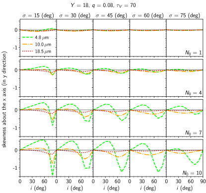
Figure 13: Image skewness about the $x$-axis, i.e. in the $y$-direction. Values $>0$ indicate skewness toward the negative $y$-axis, and values $<0$ indicate skewness toward the positive $y$-axis. Torus parameters $\hbox{$Y$}=18$, $\hbox{$q$}=0.08$, and $\hbox{$\tau_{V}$}=70$ are fixed, while $\sigma$, ${\cal N}_{0}$, and $i$ vary as indicated. The three line styles and colors encode three different wavelengths (see legend).

3.4 Morphologies of Projected Dust Maps

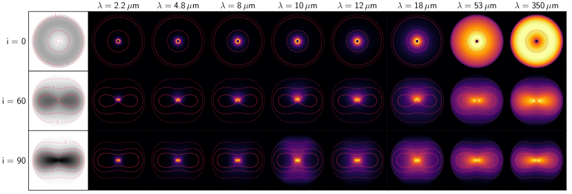
Figure 14: Torus emission maps for a model with parameters $\sigma$ = 43°, $Y$ = 18, $q$ = 0.08, $\tau_{V}$ = 70, and ${\cal N}_{0}$ = 4, shown for three viewing angles $i$ = 0°, 60°, and 90° (as rows) and for eight wavelengths between 2.2 and 350 $\mu{\rm m}$ (as columns). All maps are stretched individually and linearly. The leftmost column shows ${\cal N}$, the number of clouds along an LOS, normalized to the global maximum $\hbox{${\cal N}$}_{\rm max}=8.54$ across all viewing angles (which occurs in edge-on view). Red dotted, dashed, and solid contours outline one, three, and five clouds along an LOS, respectively. The same contours are plotted over the emission maps in a given row.

The Hypercat model cubes also contain 2D maps of the projected dust cloud distribution in the plane of the sky, $C_{d}(x,y)$. These are maps of the number of clouds along each LOS (pixel). Whenever the LOSs through the torus are optically thick, the morphology of the torus emission cannot be expected to follow the dust cloud distribution. Figure 14 shows this clearly for one model, at three viewing angles and a number of wavelengths. The leftmost column shows the underlying dust cloud distribution, with labeled contours of constant number of clouds along an LOS overplotted. Only at FIR wavelengths above $\approx\!18~{}\hbox{$\mu{\rm m}$}$ does the torus become globally optically thin, and the dust emission morphologies densely fill out the cloud number contours.

The methods developed earlier for brightness maps can be used to quantify the dust morphologies. We remind the reader that (i) the dust maps do not depend on $\tau_{V}$; (ii) they depend on ${\cal N}_{0}$ only as a multiplicative factor, i.e., $C_{d}(\hbox{${\cal N}_{0}$})=\hbox{${\cal N}_{0}$}\!\times C_{d}(\hbox{${\cal N}_{0}$}\!=\!1)$; and (iii) moment-based morphological measurements on these dust maps, such as radii of gyration and elongations, are independent of ${\cal N}_{0}$ as well. They only depend on $\sigma$, $i$, $Y$, and $q$, i.e. on the truly geometrical parameters. We can thus compare the extension of the thermal emission maps with the extension of the dust distribution map.

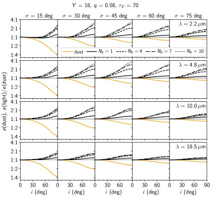
Figure 15: Elongation of the dust distribution, $e\rm(dust)$ (orange solid line below the 1:1 ratio), and the ratio of emission elongation to this dust elongation for a number of ${\cal N}_{0}$ values (black lines; see legend). Positive values indicate that the elongation of the emission is more polar than the elongation of the dust distribution. Torus parameters $\hbox{$Y$}=18$, $\hbox{$q$}=0.08$, and $\hbox{$\tau_{V}$}=70$ are fixed, while $\sigma$, $i$ and $\lambda$ vary as indicated. The vertical axis is logarithmic. Values $>1$ show elongation in the $y$-direction (polar extension), and $<1$ show elongation in the $x$-direction (equatorial extension).

Figure 15 shows as orange lines the morphological elongation of the 2D dust maps for a number of model parameter combinations. $\sigma$ (columns) and $\lambda$ (rows) vary from panel to panel. In every column the orange curve is the same, since the dust distribution does not depend on wavelength. In all cases the elongation of the dust distribution is in the equatorial direction (i.e. ratios smaller than 1:1), which is expected given the range of $\sigma$ values sampled.

The other lines show the ratio of this elongation of the emission to the elongation of the underlying dust morphology, at four different values of ${\cal N}_{0}$. In almost all cases the elongation of the emission distribution is more polar than the elongation of the associated dust distribution. The only marginal exception is at the smallest $\sigma$ and smallest ${\cal N}_{0}$. The emission-to-dust elongation ratios are higher at shorter wavelengths. At large $\sigma$ and wavelengths longer than $\sim$12 $\mu{\rm m}$ the elongations of the emission and dust morphologies are quite close to each other.

Figure 16 demonstrates spatial 2D maps of the ratio of local emission to dust content.

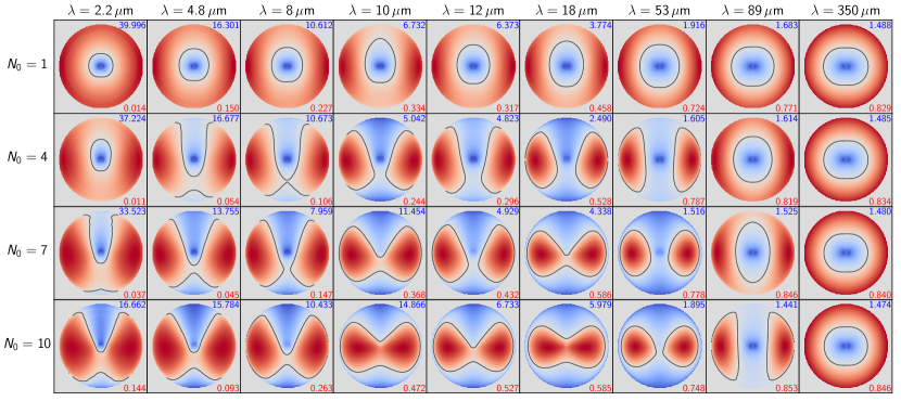
Figure 16: Ratio of emission map to dust cloud map. Regions where the fractional light emission dominates over the fractional dust content are blue, and regions where there is fractionally more dust present than emission produced are red. A single black contour line divides them. Both the input emission and dust maps were first normalized to unit sum, i.e. they are fractional maps of the total emission and total dust cloud number. Torus parameters $\hbox{$\sigma$}=43$°, $\hbox{$i$}=75$°, $\hbox{$Y$}=18$, $\hbox{$q$}=0.08$, and $\hbox{$\tau_{V}$}=70$ are fixed, while ${\cal N}_{0}$ and $\lambda$ vary as indicated. The dust cloud map is the same for every panel since its morphology does not depend on ${\cal N}_{0}$ or $\lambda$. The resulting light-to-dust ratio maps are scaled logarithmically, and the ranges above/below zero are stretched independently (symlog). The dynamic range is different in each panel; the min/max (linear) ratios are printed in the right lower/upper corners in red/blue.

The dust map is the same for all panels and corresponds to the best-fit NGC 1068 model as before, with $\hbox{$\sigma$}=43$°, $\hbox{$i$}=75$°, $\hbox{$Y$}=18$, $\hbox{$q$}=0.08$, and $\hbox{$\tau_{V}$}=70$. ${\cal N}_{0}$ and $\lambda$ vary between panels as indicated. Each panel shows the ratio (computed per pixel) of the light emission map and the generating dust map, which both were first normalized to unit sum. That is, both are fractional maps of the total emission and total dust cloud number. The scaling of the ratio maps is symmetrically logarithmic. A single black contour line divides regions where the fractional emission dominates over the fractional dust content (blue colors) from those regions where there is fractionally more dust present than light produced (red colors).

These maps give quick insight of the interplay between the global morphology of photons generated by the distribution of dust. For our model with viewing angle $i$ = 75°, i.e., tilted by 15° toward the observer, it is immediately clear that at MIR wavelength the emission has the upper hand over dust contribution in regions high above the equatorial plane of the torus, along the system axis. When ${\cal N}_{0}$ is very small, at nearly all wavelengths the emission is concentrated to a small circular region around the image center. The same is true at any value of ${\cal N}_{0}$ when the wavelength is very long (submillimeter).

4 Summary

To date only VLTI and ALMA, both interferometers, have been able to spatially resolve the IR emission from nuclear dusty environments in some nearby AGNs. In the future a number of extremely large single-dish telescopes will be pointing their 24–39 m diameter (GMT, TMT, ELT) primary mirrors at AGNs as well. They will resolve the IR emission in these sources, providing answers about the morphologies of light emission and dust distribution that are free from model assumptions. Resolved and model-free imagery is the only technique capable of breaking degeneracies intrinsic to IR radiative transfer that can produce similar SEDs from different dust geometries.

A major observational finding in recent years was that in several nearby AGNs the MIR emission resolved with VLTI appears elongated along the polar direction of the system. That is, the MIR light emanates from regions above the equatorial plane of the AGN torus. Several attempts at explaining these observations were proposed, some of which significantly deviate from simple AGN unification models.

We developed techniques based on image moments to quantify image morphology, and we show that thermal emission maps produced by simple “classical” toroidal models such as Clumpy can generate significant polar elongation in the MIR. Typical polar-to-equatorial size ratios of up to 2:1 found by interferometric observations on physical scales of several parsec are easily achievable by Clumpy torus models and can be even larger depending on sensitivity levels. We constrain the ranges of parameters that produce such elongations and find that they are rather standard. A slight tilt of the torus system axis toward the observer is enough to produce elongations compatible with many observations. We further find that it is impossible to obtain any polar elongation at small values of $\sigma$ and $i$, at smallest values of ${\cal N}_{0}$, or at wavelengths longer than $\sim$14–18 $\mu{\rm m}$. If the radial cloud distribution is compact (higher $q$ values), polar elongations are only achievable up to $\sim$5 $\mu{\rm m}$.

While the clumpy distributions that we model here fundamentally provide the optically and geometrically thick material that AGN unification calls for, and alone can account for much of the observed polar elongation, additional components may still be present, especially on larger physical scales (tens of pc). For example, extended winds (Hönig & Kishimoto, 2017; Izumi et al., 2018; Asmus, 2019) and photoionization of existing material may also contribute, including at MIR wavelengths. In some sources, such as NGC 1068, MIR interferometric data suggest that there are additional components, e.g., from a putative dusty outflow, which are extended on larger scales, or even disassociated (López-Gonzaga et al., 2014); outflows on even larger scales, and crossing to the galactic domain, are seen in submillimeter, molecular gas observations (e.g., Aalto et al., 2020; and references therein). These very extended components may not be explainable with a torus model alone, and their physical connection with the torus, or lack thereof, needs to be studied.

Evidence from radiation-hydrodynamical simulations also strongly suggests that two-component models may be preferable, especially on larger scales, where outflowing winds and “failed fountains” may provide a good fraction of the observed MIR emission on scales of tens of parsecs and be elongated in polar directions (e.g., Schartmann et al., 2014; Wada et al., 2016; Williamson et al., 2020). Note that only large dust grains could survive in such polar regions (e.g., Tazaki & Ichikawa, 2020). The full picture likely requires magnetohydrodynamics as well (Blandford & Payne, 1982; Emmering et al., 1992) given the recent direct detection of $B$-fields along the equatorial direction of the dusty torus in NGC 1068 (Lopez-Rodriguez et al., 2020). These measurements of magnetically aligned dust grains using ALMA polarization at 860 $\mu{\rm m}$ support the picture that magnetic fields up to a few parsecs contribute to the accretion flow onto active nuclei.

We also compared the emission morphologies to their generative projected (2D) dust maps. A key result is that the emission morphology does not simply trace the dust distribution in the system. Optical depth effects are important at most wavelengths, including in the MIR. In the FIR and submillimeter regimes the torus is mostly optically thin, even for a high number of clouds along the LOS. There, the observed emission does trace the underlying dust distribution.

To quantify morphologies, we advocate the use of moment-based techniques (e.g., radii of gyration) over more traditional methods (e.g., half-light radius). Moment-based morphological quantities are independent of the image brightness. Thus, in our case, maps of the dust cloud distribution are independent of ${\cal N}_{0}$ and $\tau_{V}$, since these are just multiplicative factors, and the brightness maps are independent of the total flux. Furthermore, morphological size measurements using radii of gyration provide size estimates along both axes independently, making it trivial to measure elongations. Moment-based quantities can estimate higher-order morphological quantities such as image asymmetry, skewness, and kurtosis.

In anticipation of the extremely large telescopes currently planned or under construction (GMT, TMT, ELT), and to facilitate studies of image morphology, we have introduced with Hypercat a hypercube of clumpy torus images spanning a wide range of wavelengths and model parameters. The sampled wavelengths include important NIR, MIR, FIR, and submillimeter bands. Hypercat also comprises a software suite whose key functionality is to interpolate the images continuously at any set of model parameters. Another capability of Hypercat is to simulate several observing modes, e.g., single-dish observations with PSF convolution, detector pixelization, noise modeling, and image deconvolution to recover some of the original signal in the images. The processing software may also be applied to analyze different emission models, which need not be limited to AGN tori.

In the companion Paper II we apply the capabilities of the Hypercat software to the Clumpy image hypercube and simulate observations of NGC 1068 with several single-dish telescopes (JWST, Keck, GMT, TMT, ELT) to investigate the spatial resolvability of the NIR to MIR emission. We also simulate IFU-like observations to analyze the 10-$\mu{\rm m}$ silicate emission feature. Finally, we fit directly with the Clumpy images the $K$-band image of NGC 1068 recently published by G20, deriving likely model parameters.

5 Supplementary Material and Software

The hypercubes of Clumpy images and cloud distribution maps (as a function of all model parameters and wavelengths) are provided to the community through FTP download. See Appendix A, and the User Manual, for download instructions.

We also provide the Hypercat software, which comprises user-friendly tools to operate on the hypercubes, simulate observations, and investigate morphology. All codes, scripts, and telescope pupil images can be found in the GitHub repository at https://github.com/rnikutta/hypercat/ .

The repository also contains the User Manual, several instructional Jupyter notebooks, and API documentation. The User Manual contains high-level usage examples and also showcases low-level operations that can be performed with Hypercat.

We kindly ask for citation of this paper if the reader decides to make use of any of the Hypercat data cubes, software functions, scripts, or telescope pupil images.

Appendix A Download and Verification of Model Hypercubes

Readers interested in using the Clumpy hypercubes will need to download one or more hdf5 files from https://www.clumpy.org/images/, or from the current FTP location: ftp://ftp.tuc.noirlab.edu/pub/nikutta/hypercat/. Table 3 lists the available options. The *_all.hdf5.gz file contains the image hypercube at all sampled wavelengths. This is the maximally compressed version of the hdf5 file, which must be uncompressed on the user’s computer system. To reduce the peak storage required on the target computer, both steps can be executed in one go (all commands in a single line):

⬇

lftp -e ’set net:timeout 10; cat /pub/nikutta/hypercat/hypercat_20200830_all.hdf5.gz; bye’ ftp.tuc.noirlab.edu | gunzip >

hypercat_20200830_all.hdf5

The program lftp must be installed on the target system, and 914 GB of space must be available on it (but only 271 GB of compressed data will be downloaded). The reader should also download the checksums file ftp://ftp.tuc.noirlab.edu/pub/nikutta/hypercat/hypercat_20200830.md5 file and verify the hypercube file:

⬇

# this can take 30 minutes even on a modern computer

md5sum --ignore-missing -c hypercat_20200830.md5

hypercat_20200830_all.hdf5: OK

# or on MacOS and BSD variants

md5 hypercat_20200830_all.hdf5

#... and compare the printed hash with the one in the .md5 file

The download was successful if the computed checksum is identical to the one in the MD5 sums file. The same procedure applies to the other *hdf5.gz files analogously (which hold subsets of the wavelength sampling).

Appendix B Computation, Storage Requirements, and Organization of HDF5 Model Files

The Hypercat model images are embedded within the same FOV, corresponding to the largest sampled $Y$ value, $Y_{\rm max}$. The total number of pixels in all stored brightness maps is therefore $N_{\rm pix}^{\rm img}=N_{x}\,N_{y}\times\prod_{k}N_{\theta_{k}}$, where $N_{\theta_{k}}$ is the number of sampled values per model parameter $\theta_{k}$, $k\in\{\hbox{$\sigma$},\hbox{$i$},\hbox{$Y$},\hbox{${\cal N}_{0}$},\hbox{$q$},\hbox{$\tau_{V}$},\lambda\}$, as compiled in Table 1. Thus, $\prod_{k}\!N_{\theta_{k}}$ is the total number of realized parameter combinations. If full images are stored, the total number of pixels in the hypercube is $N_{\rm pix}^{\rm img}=\left(2\,\hbox{$Y_{\rm max}$}\,\eta+1\right)^{2}\times\prod_{k}N_{\theta_{k}}$. If half-images are stored, as is the case in Hypercat because of image symmetry, then $N_{\rm pix}^{\rm img}=\left(\hbox{$Y_{\rm max}$}\,\eta+1\right)\left(2\,\hbox{$Y_{\rm max}$}\,\eta+1\right)\times\prod_{k}N_{\theta_{k}}$. That is, the number of computed pixels grows quadratically with $Y_{\rm max}$, quadratically with the image resolution per unit linear size $\eta$, and linearly with the sampling of any model parameter including wavelength. Clumpy also computes integrated dust maps during ray-tracing, and with the parameter sampling of our grid, 4000 such maps were produced (see Section 2.6 and 2.7). With half-image ray-tracing and $\eta=6$, the final number of stored pixels (images + cloud maps) is then $N_{\rm pix}^{\rm tot}=N_{\rm pix}^{\rm img}+N_{\rm pix}^{\rm cld}\approx 2.45\times 10^{11}$ pixels, which at single precision (32 bit = 4 bytes) requires $\approx 913$ GB of storage. We deliver this hypercube of half-images as a compressed HDF5 file (.hdf5.gz) of 270 GB size, and we have also produced four smaller HDF5 files with partial wavelength coverage. Table 3 lists their properties.

Such file sizes can be handled relatively easily with regard to network download and possibly even storage on a researcher’s personal workstation, but they are 1-3 orders of magnitude too large to load the entire set into memory (for instance, for the purpose of $n$-dimensional interpolation). We must therefore devise routines for slicing the hypercube along any parameter axes of interest, and for on-the-fly access to any image map within the envelope of the sampled parameter space (see User Manual for details). Together with the hypercubes, we provide functions to transparently extract full-sized (square) images via $n$-dimensional interpolation on the hypercube and (automatic) left-right mirroring about the $y$-axis.

The Hierarchical Data Format version 5 (HDF5) is well established for packaging structured and heterogeneous data sets and metadata, and it is agnostic about the operating system. We use the Python package h5py to construct our hypercubes, and the Hypercat software uses h5py to access said data. HDF implementations in other languages are readily available. The structure of every Hypercat HDF5 file is simple. Listing 1 shows the hierarchy tree of the main HDF5 file released with this paper.

Listing 1: Structure of a Hypercat HDF5 file. Some nonessential attributes omitted for clarity.

⬇

/Nhypercubes : 2

/hypercubenames : [’imgdata’, ’clddata’]

/imgdata/ : (group)

/Nparam : 9

/paramnames : [’sig’,’i’,’Y’,’N’,’q’,’tv’,’wave’,’x’,’y’]

/theta : [[15,30,45,60,75],[0,10,20,30,40,50,60,70,80,90],...]

/hypercubeshape : [5,10,16,12,5,7,25,121,241]

/hypercube : (9-d array)

/clddata/ : (group)

/Nparam : 6

/paramnames : [’sig’,’i’,’Y’,’q’,’x’,’y’]

/theta : [[15,30,45,60,75],[0,10,20,30,40,50,60,70,80,90],...]

/hypercubeshape : [5,10,16,5,121,241]

/hypercube : (6-d array)

There are Nhypercube=2 hypercubes in the file. Their names are imgdata and clddata, each stored in a separate HDF group. Group imgdata contains the thermal emission maps, stored in a 9-dimensional ($\hbox{$\sigma$},\hbox{$i$},\hbox{$Y$},\hbox{${\cal N}_{0}$},\hbox{$q$},\hbox{$\tau_{V}$},\lambda,x,y$) array imgdata/hypercube. Several other small data sets of auxiliary information are also stored inside the group, e.g., the mapping of parameter values to the hypercube grid vertices (theta). The hypercube shape is given in hypercubeshape, and every array axis corresponds to one list in theta, and to one parameter name in paramnames. theta in the listing above shows the sampling of the parameters sig and i, which is the torus angular thickness $\sigma$, and of the viewing angle $i$. Other parameter samplings are truncated here for brevity. The clddata group does the same for the 2D maps of cloud number along the LOS. These maps do not depend on wavelength and cloud optical depth $\tau_{V}$, and ${\cal N}_{0}$ is just a multiplicative factor (see Section 2.6); thus, their hypercube is 6-dimensional ($\hbox{$\sigma$},\hbox{$i$},\hbox{$Y$},\hbox{$q$},x,y$).

Appendix C Morphology

Various methods exist to quantify image morphology. One very powerful approach, due to its generality, is the framework of image moments. For digitized images $I(x,y)$ with $x$ and $y$ pixel indices, the $(p+q)$-order raw or geometric moment is defined as

$$M_{pq}=\sum_{x}\sum_{y}I(x,y)\,x^{p}\,y^{q},$$ (C1)

with a standard power basis. Other bases, e.g., orthogonal functions, Zernike polynomials, etc., are possible and are being used in numerous applications. For binary images the raw moment $M_{00}$ is the area (sum) of the one-valued pixels. For grayscale images, in the astronomical context, it is the total light contained in all pixels.

Figure 17 demonstrates the effects of various image operations (using 2D Gaussians as images) on the measured moments, from left to right and top to bottom: (a) translation, (b) stretching, (c) scaling, (d) & (e) skewing, and (f) rotation.

Panel (a) shows a 2D Gaussian with $\sigma_{x}=5,\,\sigma_{y}=10$ pixels (in a $101\times 101$ pixel frame) being shifted from $y_{0}=-20$ through $+20$ pixels, and the corresponding centroid locations $\bar{x}$ (not changing) and $\bar{y}$ (changing).

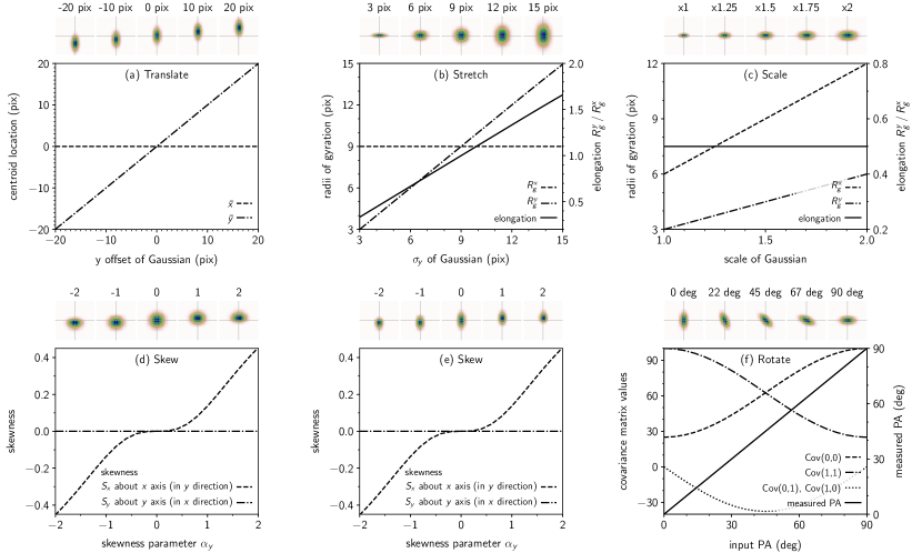
Figure 17: The effects on morphological quantities of various image operations, measured on 2D Gaussians. Five small images per operation demonstrate the effect. The large panels show the measurements as continuous functions. Solid lines use the right $y$-axis. (a) Translation, measured via centroid location $\bar{x},\bar{y}$. (b) Stretching in the $y$-direction, measured via radii of gyration $R_{g}^{x}$, $R_{g}^{y}$. The $y$ elongation of the Gaussian is $e=R_{g}^{y}\,/\,R_{g}^{x}$ (solid line). (c) Scaling of the morphology, measured via radii of gyration. The elongation remains constant. (d) Skewness about $x$-axis (i.e., in the $y$-direction) of a circular Gaussian, measured via third-order moments. $\alpha_{y}$ controls the skew in the $y$-direction of the 2D skew-normal distribution. $\alpha_{x}$ is fixed at 0, i.e. no skew. (e) Same as (d) but of a vertically elongated 2D Gaussian. Skewness in the $y$-direction is independent of the distribution of pixels in the $x$-direction. (f) Rotation of position angle, measured via image covariance matrix. The four matrix elements are plotted as nonsolid lines. The measured ${\rm PA}$ (solid line) is observed from the image (in degrees east from north, with north up).

Panel (b), left axis, shows how $R_{g}^{y}$ grows when the 2D Gaussian is being stretched vertically, and in panel (c), left axis, shows how $R_{g}^{x}$ and $R_{g}^{y}$ both increase linearly with the increasing scale of a 2D Gaussian. This linear behavior makes radii of gyration very well suited for measuring the characteristic sizes of the pixel distribution.

Panel (b), right axis, also shows how elongation is measured, using a 2D Gaussian as an example whose $x$-size $\sigma_{x}$ is 9 pixels always, while $\sigma_{y}$ is varied from 3 to 15 pixels. That is, the Gaussian spans a range of aspect ratios from 1:3 to 5:3. The measured elongation (solid line) grows linearly with $\sigma_{y}$.

Panels (d) and (e) show how skewness can be measured using Eqns. (11). For this demonstration we use the 2D version (i.e. $k=2$) of the multivariate skew-normal distribution as defined by Azzalini & Dalla Valle (1996), with density function

$$f(z)=2\,\phi_{k}(z;\Omega)\,\Phi(\alpha^{\mathrm{T}}z),\quad(z\in\mathbb{R}^{k}),$$ (C2)

where $\phi(\cdot)$ is the $k$-dimensional normal density with zero mean and correlation matrix $\Omega$, $\Phi(\cdot)$ is the $N(0,1)$ distribution function, and $\alpha$ is a $k$-dimensional vector of skewness coefficients. In our case, $\alpha=(\alpha_{x}=0,\alpha_{y})$. In panel (d) a symmetric 2D Gaussian is modified by changing the skewness parameter $\alpha_{y}$. The skewness $S_{x}$ about the $x$-axis, i.e., in the $y$-direction, changes as a result, while $S_{y}$ remains constant. In panel (e) the same operations are applied to an initially elongated 2D Gaussian; the resulting $S_{x}$ curve is identical, i.e. the skewness about an axis is independent of the distribution of pixels with respect to the other axis.

C.1 More on Image Moments

Versions of central moments that are invariant to both translation and scale operations are possible by properly normalizing the central moments

$$\eta_{pq}=\frac{\mu_{pq}}{\mu_{00}^{\left(\displaystyle 1+\frac{p+q}{2}\right)}}\qquad\forall\ p+q\geq 2.$$ (C3)

Scale invariance in this context means similitude, which is the resizing of a 2D shape while preserving its proportions. Invariants simultaneously under translation, scaling, and rotation can be defined as combinations of moments (Hu, 1962; Reiss, 1991; Flusser & Suk, 1993). For our applications we do not need to concern ourselves with rotation, since we are always able to set the positional angle ${\rm PA}=0$° in our images. Some useful observations on moments:

1. Zero-order central and raw moments are identical: $\mu_{00}=M_{00}$.

2. First-order central moments are zero: $\mu_{10}=\mu_{01}=0$.

3. Second-order central moments $\mu_{20}$ and $\mu_{02}$ measure the distribution of mass w.r.t. the image axes, i.e. can be used to measure source elongation and orientation (see Section 3.2.3).

4. Third- and fourth-order central moments can measure higher-order image properties such as skew/asymmetry (see Section 3.3) and kurtosis/peakedness (see Section C.3).

Note that some of the moment-based functionality is available in the photutils package for Python. Unfortunately, at the time of writing, there exist several incompatibilities between Astropy’s models package, the scikit-image module, and photutils. For that reason, we rely on our own moment-based implementation. It is straightforward to use, is performant, and does not have many dependencies. This morphology module is part of the Hypercat source code distribution.

C.2 Image Elongation via Covariance Matrix

An equivalent method exists to measure the elongation $e$ of a morphology using the eigenvalues of the image covariance matrix. The eigenvalues and eigenvectors of the covariance matrix $\Sigma$ of an image $I$ encode the magnitude and direction of the principal components of $I$, i.e. the 2D extension of the pixel distribution. In our case we can always set the position angle to ${\rm PA}=0$°, i.e., we are only interested in elongations along the orthogonal $\mathbf{e}_{x}$ and $\mathbf{e}_{y}$ directions of the image. Thus, the eigenvalues measure the magnitude of the pixel distribution along the $x$ and $y$-directions.

The covariance matrix $\Sigma$ can be computed in several ways, e.g., from second-order central moments

$$\Sigma\equiv\mathrm{Cov}[I(x,y)]=\begin{bmatrix}\mu^{\prime}_{20}&\mu^{\prime}_{11}\\ \mu^{\prime}_{11}&\mu^{\prime}_{02}\end{bmatrix},$$ (C4)

where $\mu^{\prime}_{\rm pq}=\mu_{\rm pq}/\mu_{00}$. The eigenvalues of $\Sigma$ can be obtained analytically, or conveniently by computer packages (e.g., linalg.eigvals in numpy). The elongation of the intensity distribution in $I(x,y)$ is then the square root of their ratio, i.e. $e=\sqrt{\lambda_{y}/\lambda_{x}}$. The same elongation can also be computed using the gyration radii as $e=R_{g}^{y}\,/\,R_{g}^{x}$. Thus, $\lambda_{x}=(R_{g}^{x})^{2}$ and $\lambda_{y}=(R_{g}^{y})^{2}$.

C.3 Kurtosis

Kurtosis is a fourth-order measure that expresses the “peakedness” of a distribution

$$K_{\!x}=\frac{\mu_{40}}{\mu_{20}^{2}}-3,\qquad K_{\!y}=\frac{\mu_{04}}{\mu_{02}^{2}}-3.$$ (C5)

In the context of image morphology, it can be used to quantify the compactness of the emission pattern. $K_{x,y}$ are zero for a Gaussian distribution, greater than zero for distributions more peaked than Gaussians, and less than zero for flatter distributions.

C.4 Image Orientation

During our analysis of image morphology in Section 3 we could set the image orientation to ${\rm PA}=0$° in all cases. Should, however, the need arise to measure the orientation of the dominant image component, Hypercat can do this via the covariance matrix of the image and its eigenvectors:

⬇

from hypercat import imageops, morphology

cube = ... # load cube as described e.g. in the HYPERCAT User Manual

img = cube(vec) # with parameter vector suitable for cube

rotimg = imageops.rotateImage(img,’42 deg’) # PA=42 deg as example

morphology.get_angle(rotimg)

42.0011 # PA measured from image

C.5 Half-light Radius

A circular aperture with half-light radius $R_{\rm HL}$ contains half of the flux in an image $I$, such that (see, e.g., Burtscher et al., 2013)

$$\frac{1}{F_{\rm tot}}\int\limits_{0}^{R_{\rm HL}}\!\!\hbox{${d}$}r\,I\,2\pi r=\frac{1}{2},$$ (C6)

where $R_{\rm HL}$ is the root of this equation. The solution is not unique if the circle need not be centered in the image.

C.6 Gini Coefficient

Figure 18 shows the smallest and largest morphologies within the parameter space from Figure 10

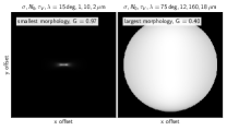
Figure 18: Smallest and largest morphologies within the parameter space from Fig 10. Linear scale. $Y=18$, $q=0$, and $i=90$° are identical in both cases. Left: smallest / most compact emission map. Gini index $G=0.97$, elongation $e=R_{g}^{y}/R_{g}^{x}=0.31$. Right: largest / most extended emission map. Gini index $G=0.4$, elongation $e=1.0$.

References

- Aalto et al. (2020) Aalto, S., Falstad, N., Muller, S., et al. 2020, A&A, 640, A104, doi: 10.1051/0004-6361/202038282
- Alonso-Herrero et al. (2011) Alonso-Herrero, A., Ramos Almeida, C., Mason, R., et al. 2011, ApJ, 736, 82, doi: 10.1088/0004-637X/736/2/82
- Alonso-Herrero et al. (2018) Alonso-Herrero, A., Pereira-Santaella, M., García-Burillo, S., et al. 2018, ApJ, 859, 144, doi: 10.3847/1538-4357/aabe30
- Alonso-Herrero et al. (2019) Alonso-Herrero, A., García-Burillo, S., Pereira-Santaella, M., et al. 2019, A&A, 628, A65, doi: 10.1051/0004-6361/201935431
- Antonucci (1993) Antonucci, R. 1993, ARA&A, 31, 473, doi: 10.1146/annurev.aa.31.090193.002353
- Asensio Ramos & Ramos Almeida (2009) Asensio Ramos, A., & Ramos Almeida, C. 2009, ApJ, 696, 2075, doi: 10.1088/0004-637X/696/2/2075
- Asmus (2019) Asmus, D. 2019, MNRAS, 489, 2177, doi: 10.1093/mnras/stz2289
- Astropy Collaboration et al. (2013) Astropy Collaboration, Robitaille, T. P., Tollerud, E. J., et al. 2013, A&A, 558, A33, doi: 10.1051/0004-6361/201322068
- Audibert et al. (2017) Audibert, A., Riffel, R., Sales, D. A., Pastoriza, M. G., & Ruschel-Dutra, D. 2017, MNRAS, 464, 2139, doi: 10.1093/mnras/stw2477
- Azzalini & Dalla Valle (1996) Azzalini, A., & Dalla Valle, A. 1996, Biometrika, 83, 715, doi: 10.1093/biomet/83.4.715
- Barvainis (1987) Barvainis, R. 1987, ApJ, 320, 537, doi: 10.1086/165571
- Blandford & Payne (1982) Blandford, R. D., & Payne, D. G. 1982, MNRAS, 199, 883, doi: 10.1093/mnras/199.4.883
- Burtscher et al. (2013) Burtscher, L., Meisenheimer, K., Tristram, K. R. W., et al. 2013, A&A, 558, A149, doi: 10.1051/0004-6361/201321890
- Collette et al. (2019) Collette, A., et al. 2019, h5py: HDF5 for Python. http://www.h5py.org/
- Combes et al. (2019) Combes, F., García-Burillo, S., Audibert, A., et al. 2019, A&A, 623, A79, doi: 10.1051/0004-6361/201834560
- Dorodnitsyn & Kallman (2017) Dorodnitsyn, A., & Kallman, T. 2017, ApJ, 842, 43, doi: 10.3847/1538-4357/aa7264
- Draine (2003) Draine, B. T. 2003, ApJ, 598, 1017, doi: 10.1086/379118
- Efstathiou & Rowan-Robinson (1995) Efstathiou, A., & Rowan-Robinson, M. 1995, MNRAS, 273, 649
- Elitzur & Netzer (2016) Elitzur, M., & Netzer, H. 2016, MNRAS, 459, 585, doi: 10.1093/mnras/stw657
- Elitzur & Shlosman (2006) Elitzur, M., & Shlosman, I. 2006, ApJ, 648, L101, doi: 10.1086/508158
- Emmering et al. (1992) Emmering, R. T., Blandford, R. D., & Shlosman, I. 1992, ApJ, 385, 460, doi: 10.1086/170955
- Fan et al. (2016) Fan, L., Han, Y., Nikutta, R., Drouart, G., & Knudsen, K. K. 2016, ApJ, 823, 107, doi: 10.3847/0004-637X/823/2/107
- Feltre et al. (2012) Feltre, A., Hatziminaoglou, E., Fritz, J., & Franceschini, A. 2012, MNRAS, 426, 120, doi: 10.1111/j.1365-2966.2012.21695.x
- Flusser & Suk (1993) Flusser, J., & Suk, T. 1993, Pattern Recognition, 26, 167 , doi: https://doi.org/10.1016/0031-3203(93)90098-H
- Fritz et al. (2006) Fritz, J., Franceschini, A., & Hatziminaoglou, E. 2006, MNRAS, 366, 767, doi: 10.1111/j.1365-2966.2006.09866.x
- Fuller et al. (2016) Fuller, L., Lopez-Rodriguez, E., Packham, C., et al. 2016, MNRAS, 462, 2618, doi: 10.1093/mnras/stw1780
- Gallimore et al. (2016) Gallimore, J. F., Elitzur, M., Maiolino, R., et al. 2016, ApJ, 829, L7, doi: 10.3847/2041-8205/829/1/L7
- García-Bernete et al. (2019) García-Bernete, I., Ramos Almeida, C., Alonso-Herrero, A., et al. 2019, MNRAS, 486, 4917, doi: 10.1093/mnras/stz1003
- García-Burillo et al. (2014) García-Burillo, S., Combes, F., Usero, A., et al. 2014, A&A, 567, A125, doi: 10.1051/0004-6361/201423843
- García-Burillo et al. (2016) García-Burillo, S., Combes, F., Ramos Almeida, C., et al. 2016, ApJ, 823, L12, doi: 10.3847/2041-8205/823/1/L12
- García-Burillo et al. (2019) García-Burillo, S., Combes, F., Ramos Almeida, C., et al. 2019, A&A, 632, A61, doi: 10.1051/0004-6361/201936606
- Gautier (2014-2019) Gautier, L. 2014-2019, r2py. https://rpy2.bitbucket.io/
- Gini (1921) Gini, C. 1921, The Economic Journal, 31, 124. http://www.jstor.org/stable/2223319
- González-Martín et al. (2019a) González-Martín, O., Masegosa, J., García-Bernete, I., et al. 2019a, ApJ, 884, 10, doi: 10.3847/1538-4357/ab3e6b
- González-Martín et al. (2019b) —. 2019b, ApJ, 884, 11, doi: 10.3847/1538-4357/ab3e4f
- Goulding et al. (2012) Goulding, A. D., Alexander, D. M., Bauer, F. E., et al. 2012, ApJ, 755, 5, doi: 10.1088/0004-637X/755/1/5
- Graham et al. (2005) Graham, A. W., Driver, S. P., Petrosian, V., et al. 2005, AJ, 130, 1535, doi: 10.1086/444475
- Granato & Danese (1994) Granato, G. L., & Danese, L. 1994, MNRAS, 268, 235
- Gravity Collaboration et al. (2020) Gravity Collaboration, Pfuhl, O., Davies, R., et al. 2020, A&A, 634, A1, doi: 10.1051/0004-6361/201936255
- Hahn (2005) Hahn, T. 2005, Computer Physics Communications, 168, 78 , doi: https://doi.org/10.1016/j.cpc.2005.01.010
- Harris et al. (2020) Harris, C. R., Millman, K. J., van der Walt, S. J., et al. 2020, Nature, 585, 357, doi: 10.1038/s41586-020-2649-2
- Hönig et al. (2006) Hönig, S. F., Beckert, T., Ohnaka, K., & Weigelt, G. 2006, A&A, 452, 459, doi: 10.1051/0004-6361:20054622
- Hönig & Kishimoto (2017) Hönig, S. F., & Kishimoto, M. 2017, ApJ, 838, L20, doi: 10.3847/2041-8213/aa6838
- Hönig et al. (2012) Hönig, S. F., Kishimoto, M., Antonucci, R., et al. 2012, ApJ, 755, 149, doi: 10.1088/0004-637X/755/2/149
- Hönig et al. (2013) Hönig, S. F., Kishimoto, M., Tristram, K. R. W., et al. 2013, ApJ, 771, 87, doi: 10.1088/0004-637X/771/2/87
- Hu (1962) Hu, M.-K. 1962, IRE Transactions on Information Theory, 8, 179, doi: 10.1109/TIT.1962.1057692
- Hunter (2007) Hunter, J. D. 2007, Computing In Science & Engineering, 9, 90, doi: 10.1109/MCSE.2007.55
- Ichikawa et al. (2015) Ichikawa, K., Packham, C., Ramos Almeida, C., et al. 2015, ApJ, 803, 57, doi: 10.1088/0004-637X/803/2/57
- Imanishi et al. (2016) Imanishi, M., Nakanishi, K., & Izumi, T. 2016, ApJ, 822, L10, doi: 10.3847/2041-8205/822/1/L10
- Imanishi et al. (2018) Imanishi, M., Nakanishi, K., Izumi, T., & Wada, K. 2018, ApJ, 853, L25, doi: 10.3847/2041-8213/aaa8df
- Impellizzeri et al. (2019) Impellizzeri, C. M. V., Gallimore, J. F., Baum, S. A., et al. 2019, ApJ, 884, L28, doi: 10.3847/2041-8213/ab3c64
- Izumi et al. (2018) Izumi, T., Wada, K., Fukushige, R., Hamamura, S., & Kohno, K. 2018, ApJ, 867, 48, doi: 10.3847/1538-4357/aae20b
- Jaffe et al. (2004) Jaffe, W., Meisenheimer, K., Röttgering, H. J. A., et al. 2004, Nature, 429, 47, doi: 10.1038/nature02531
- Krolik & Begelman (1988) Krolik, J. H., & Begelman, M. C. 1988, ApJ, 329, 702, doi: 10.1086/166414
- Leftley et al. (2018) Leftley, J. H., Tristram, K. R. W., Hönig, S. F., et al. 2018, ApJ, 862, 17, doi: 10.3847/1538-4357/aac8e5
- Levenson et al. (2007) Levenson, N. A., Sirocky, M. M., Hao, L., et al. 2007, ApJ, 654, L45, doi: 10.1086/510778
- López-Gonzaga et al. (2016) López-Gonzaga, N., Burtscher, L., Tristram, K. R. W., Meisenheimer, K., & Schartmann, M. 2016, A&A, 591, A47, doi: 10.1051/0004-6361/201527590
- López-Gonzaga et al. (2014) López-Gonzaga, N., Jaffe, W., Burtscher, L., Tristram, K. R. W., & Meisenheimer, K. 2014, A&A, 565, A71, doi: 10.1051/0004-6361/201323002
- Lopez-Rodriguez et al. (2018) Lopez-Rodriguez, E., Fuller, L., Alonso-Herrero, A., et al. 2018, ApJ, 859, 99, doi: 10.3847/1538-4357/aabd7b
- Lopez-Rodriguez et al. (2020) Lopez-Rodriguez, E., Alonso-Herrero, A., García-Burillo, S., et al. 2020, ApJ, 893, 33, doi: 10.3847/1538-4357/ab8013
- Markowitz et al. (2014) Markowitz, A. G., Krumpe, M., & Nikutta, R. 2014, MNRAS, 439, 1403, doi: 10.1093/mnras/stt2492
- Mateos et al. (2017) Mateos, S., Carrera, F. J., Barcons, X., et al. 2017, ApJ, 841, L18, doi: 10.3847/2041-8213/aa7268
- Mathis et al. (1977) Mathis, J. S., Rumpl, W., & Nordsieck, K. H. 1977, ApJ, 217, 425, doi: 10.1086/155591
- Mor et al. (2009) Mor, R., Netzer, H., & Elitzur, M. 2009, ApJ, 705, 298, doi: 10.1088/0004-637X/705/1/298
- Natta & Panagia (1984) Natta, A., & Panagia, N. 1984, ApJ, 287, 228, doi: 10.1086/162681
- Nenkova et al. (2002) Nenkova, M., Ivezić, Ž., & Elitzur, M. 2002, ApJ, 570, L9, doi: 10.1086/340857
- Nenkova et al. (2008a) Nenkova, M., Sirocky, M. M., Ivezić, Ž., & Elitzur, M. 2008a, ApJ, 685, 147, doi: 10.1086/590482
- Nenkova et al. (2008b) Nenkova, M., Sirocky, M. M., Nikutta, R., Ivezić, Ž., & Elitzur, M. 2008b, ApJ, 685, 160, doi: 10.1086/590483
- Nikutta et al. (2009) Nikutta, R., Elitzur, M., & Lacy, M. 2009, ApJ, 707, 1550, doi: 10.1088/0004-637X/707/2/1550
- Nikutta et al. (2021) Nikutta, R., Lopez-Rodriguez, R., Ichikawa, K., et al. 2021, ApJ (Paper II)
- Ossenkopf et al. (1992) Ossenkopf, V., Henning, T., & Mathis, J. S. 1992, A&A, 261, 567
- Petrosian (1976) Petrosian, V. 1976, ApJ, 209, L1, doi: 10.1086/182253
- Pier & Krolik (1992) Pier, E. A., & Krolik, J. H. 1992, ApJ, 401, 99, doi: 10.1086/172042
- Pier & Krolik (1993) —. 1993, ApJ, 418, 673, doi: 10.1086/173427
- Poncelet et al. (2006) Poncelet, A., Perrin, G., & Sol, H. 2006, A&A, 450, 483, doi: 10.1051/0004-6361:20053608
- Price-Whelan et al. (2018) Price-Whelan, A. M., Sipőcz, B. M., Günther, H. M., et al. 2018, AJ, 156, 123, doi: 10.3847/1538-3881/aabc4f
- Prieto et al. (2014) Prieto, M. A., Mezcua, M., Fernández-Ontiveros, J. A., & Schartmann, M. 2014, MNRAS, 442, 2145, doi: 10.1093/mnras/stu1006
- Privon et al. (2012) Privon, G. C., Baum, S. A., O’Dea, C. P., et al. 2012, ApJ, 747, 46, doi: 10.1088/0004-637X/747/1/46
- Raban et al. (2009) Raban, D., Jaffe, W., Röttgering, H., Meisenheimer, K., & Tristram, K. R. W. 2009, MNRAS, 394, 1325, doi: 10.1111/j.1365-2966.2009.14439.x
- Ramos Almeida et al. (2011) Ramos Almeida, C., Levenson, N. A., Alonso-Herrero, A., et al. 2011, ApJ, 731, 92, doi: 10.1088/0004-637X/731/2/92
- Reiss (1991) Reiss, T. H. 1991, IEEE Transactions on Pattern Analysis and Machine Intelligence, 13, 830, doi: 10.1109/34.85675
- Ricci et al. (2017) Ricci, C., Assef, R. J., Stern, D., et al. 2017, ApJ, 835, 105, doi: 10.3847/1538-4357/835/1/105
- Sales et al. (2015) Sales, D. A., Robinson, A., Axon, D. J., et al. 2015, ApJ, 799, 25, doi: 10.1088/0004-637X/799/1/25
- Schartmann et al. (2008) Schartmann, M., Meisenheimer, K., Camenzind, M., et al. 2008, A&A, 482, 67, doi: 10.1051/0004-6361:20078907
- Schartmann et al. (2014) Schartmann, M., Wada, K., Prieto, M. A., Burkert, A., & Tristram, K. R. W. 2014, MNRAS, 445, 3878, doi: 10.1093/mnras/stu2020
- Siebenmorgen et al. (2015) Siebenmorgen, R., Heymann, F., & Efstathiou, A. 2015, A&A, 583, A120, doi: 10.1051/0004-6361/201526034
- Sirocky et al. (2008) Sirocky, M. M., Levenson, N. A., Elitzur, M., Spoon, H. W. W., & Armus, L. 2008, ApJ, 678, 729, doi: 10.1086/586727
- Stalevski et al. (2017) Stalevski, M., Asmus, D., & Tristram, K. R. W. 2017, MNRAS, 472, 3854, doi: 10.1093/mnras/stx2227
- Stalevski et al. (2012) Stalevski, M., Fritz, J., Baes, M., Nakos, T., & Popović, L. Č. 2012, MNRAS, 420, 2756, doi: 10.1111/j.1365-2966.2011.19775.x
- Stalevski et al. (2019) Stalevski, M., Tristram, K. R. W., & Asmus, D. 2019, MNRAS, 484, 3334, doi: 10.1093/mnras/stz220
- Tazaki & Ichikawa (2020) Tazaki, R., & Ichikawa, K. 2020, ApJ, 892, 149, doi: 10.3847/1538-4357/ab72f6
- Thompson et al. (2009) Thompson, G. D., Levenson, N. A., Uddin, S. A., & Sirocky, M. M. 2009, ApJ, 697, 182, doi: 10.1088/0004-637X/697/1/182
- Tristram et al. (2014) Tristram, K. R. W., Burtscher, L., Jaffe, W., et al. 2014, A&A, 563, A82, doi: 10.1051/0004-6361/201322698
- Tristram et al. (2007) Tristram, K. R. W., Meisenheimer, K., Jaffe, W., et al. 2007, A&A, 474, 837, doi: 10.1051/0004-6361:20078369
- Urry & Padovani (1995) Urry, C. M., & Padovani, P. 1995, PASP, 107, 803, doi: 10.1086/133630
- Vinković et al. (2003) Vinković, D., Ivezić, Ž., Miroshnichenko, A. S., & Elitzur, M. 2003, MNRAS, 346, 1151, doi: 10.1111/j.1365-2966.2003.07159.x
- Virtanen et al. (2020) Virtanen, P., Gommers, R., Oliphant, T. E., et al. 2020, Nature Methods, 17, 261, doi: 10.1038/s41592-019-0686-2
- Wada (2012) Wada, K. 2012, ApJ, 758, 66, doi: 10.1088/0004-637X/758/1/66
- Wada et al. (2016) Wada, K., Schartmann, M., & Meijerink, R. 2016, ApJ, 828, L19, doi: 10.3847/2041-8205/828/2/L19
- Ward et al. (2014-2019) Ward, I., et al. 2014-2019, urwid: Console user interface library for Python. http://urwid.org/index.html
- Williamson et al. (2020) Williamson, D., Hönig, S., & Venanzi, M. 2020, ApJ, 897, 26, doi: 10.3847/1538-4357/ab989e
- Xie et al. (2016) Xie, Y., Nikutta, R., Hao, L., & Li, A. 2016, Planet. Space Sci., 133, 23, doi: 10.1016/j.pss.2016.05.009