RMPs for Safe Impedance Control in Contact-Rich Manipulation

Abstract

Variable impedance control in operation-space is a promising approach to learning contact-rich manipulation behaviors. One of the main challenges with this approach is producing a manipulation behavior that ensures the safety of the arm and the environment. Such behavior is typically implemented via a reward function that penalizes unsafe actions (e.g. obstacle collision, joint limit extension), but that approach is not always effective and does not result in behaviors that can be reused in slightly different environments. We show how to combine Riemannian Motion Policies, a class of policies that dynamically generate motion in the presence of safety and collision constraints, with variable impedance operation-space control to learn safer contact-rich manipulation behaviors.

I Introduction

Learning autonomous contact-rich manipulation behavior is a critical challenge for robotics; indeed, the very purpose of a robot is often to make contact with the environment in order to manipulate it. However, contact-rich behavior is challenging—robots must be able to reason about sudden constraints when contacting target objects and model the unknown dynamics of the objects they are manipulating, all the while respecting joint limit and collision constraints.

To address these issues, Martin-Martin et al. [1] discuss the advantages of formulating the task in the robot’s end-effector space. They propose the use of variable impedance control in end-effector space (VICES), which defines the robot’s actions in terms of displacements and compliance of the end-effector. The VICES commands are then translated back as lower-level torque commands to the joints in the arm by an operational-space impedance controller (OSC). When training an agent using reinforcement learning, the policy is trained to output actions in the VICES action-space, directly controlling end-effector behavior, and thus can manage the discontinuous mode-changes made at contact using the compliance component of the space.

While the VICES modality serves as a useful layer of abstraction for learning and transfer, the agent loses the ability to reason about the configuration of the rest of its arm in relation to the environment. This can lead to routine hyperextension and collisions during and after training, which are undesirable and potentially dangerous. The problem of safe variable impedance control has therefore not yet been solved robustly [2].

In this paper, we study the problem of safely learning contact-rich manipulation behavior. We present RMP-VICES, a principled way to incorporate well-defined collision and joint-limit avoidance behavior into the robot’s control system prior to the start of learning. We leverage Riemannian motion policies (RMPs), which allow a user to specify different behaviors in more convenient ‘task’ manifolds and then synthesize them [3, 4]. Most importantly, RMPs have a mechanism (the Riemannian metric of these task manifolds) for designating the priority of these behaviors, which can vary based on the current position and velocity of the arm. We reformulate the VICES impedance controller as an attraction-type Riemannian motion policy, and synthesize it with pre-defined obstacle avoidance and a joint limit behavior [4].

We verify the efficacy of our approach by demonstrating that RMP-VICES is comparably performant to state-of-the-art learning-based manipulation algorithms while largely preventing unsafe behavior. We do so by training a 7DOF Kinova Jaco 2 on three different simulated domains and analyzing the frequency and severity of collision and joint limit events that occur over the course of learning. Afterwards, we run the trained agents in the same domains with randomly-placed obstacles to evaluate RMP-VICES’s ability to adapt to obstacles not present in training. RMP-VICES reduces the number of collision by up to $\sim 50\%$ and joint limit events by up to $\sim 90\%$ in all of these domains with only a moderate impact on task performance.

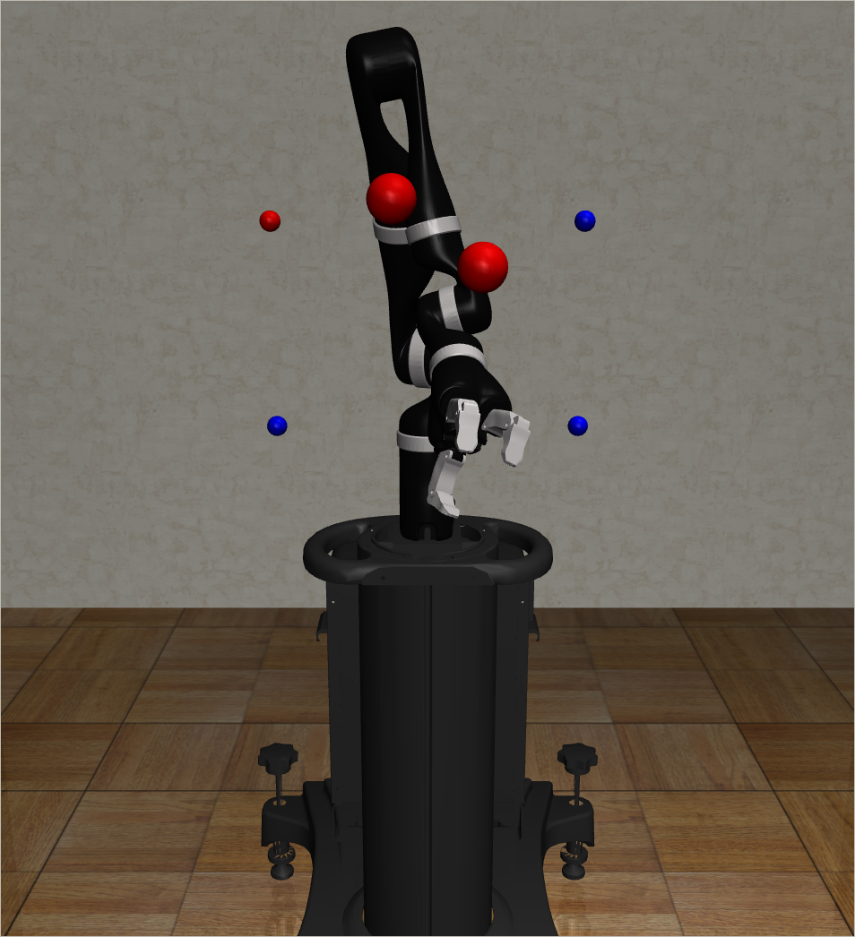
(a) Traj-follow. env.

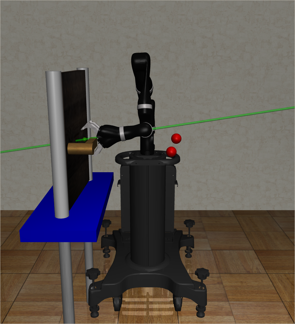
(b) Door-open. env.

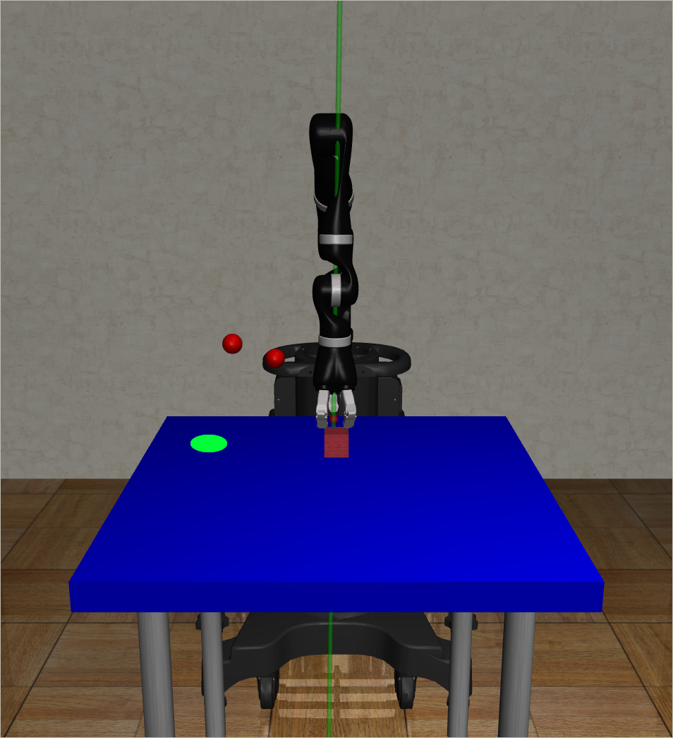
(c) Block-push. env.

Figure 1: Instances of task environments with randomly-generated obstacles (red spheres).

II Background

II-A Reinforcement Learning

A Markov Decision process $\mathcal{M}$ is given by a tuple $(\mathcal{S,A,R,T,\gamma})$. An agent receives scalar reward $r_{t}$ for taking action $a\in\mathcal{A}$ in state $s\in\mathcal{S}$ according to $\mathcal{R}(s,a)$. The state evolves according to the transition function $\mathcal{T}(s,a)$; in our setting $\mathcal{S}$ and $\mathcal{A}$ are continuous spaces. The goal of reinforcement learning is to find a policy $\pi$ which maximizes the expected discounted return

$$\max_{\theta}\mathop{\large{\mathbb{E}}}_{\mathcal{M},\pi_{\theta}}\left[\sum_{t}\gamma^{t}r_{t}\right],$$ (1)

where $\gamma$ is a discount factor. Policy search methods are a family of algorithms that search directly over a space of parameterized policies.

II-B Variable Impedance Control in End-Effector Space

VICES enables agents to use end-effector space ($\mathsf{SE(3)}$) and compliance of the end-effector as the action space of the agent. More formally, VICES defines an action $a=(\Delta x,k^{p}_{pos},k^{p}_{ori})\in\mathcal{A}=\mathsf{SE(3)}\times\mathbb{R}^{3}\times\mathbb{R}^{3}$, where $k^{p}_{pos}$ and $k^{p}_{ori}$ are vector representations of stiffness matrices in an impedance controller.

In a single timestep, $\Delta x$ is composed with the current end-effector position to produce desired setpoints $p_{des}$ and $R_{des}$. The corresponding joint torques $\tau$ are then computed using Khatib’s formulation of operation space control [5, 6]:

$$\tau= J^{T}_{pos}[\Lambda^{pos}[k^{p}_{pos}(p_{des}-p)-k_{v}^{pos}v]]+$$ (2)

$$J^{T}_{ori}[\Lambda^{ori}[e_{r}(R_{des},R)-k_{v}^{ori}\omega]],$$

where $J_{pos}$ and $J_{ori}$ are the Jacobians associated with the FK map to end-effector position $p$ and orientation $R$, $\Lambda^{pos}$ and $\Lambda^{ori}$ the corresponding end-effector inertia matrices, and $v$ and $\omega$ the velocity and angular velocity of the end-effector. We compute damping matrices $k_{v}^{pos}$ and $k_{v}^{ori}$ so that the system is critically damped relative to given $k^{p}_{pos}$ and $k^{p}_{ori}$ as chosen by the agent. $e_{r}$ is an error on $\mathsf{SO(3)}$ that can be used for impedance controllers [7]; see section III-B.

The greatest strength and weakness of VICES is that the control signal (actions) $a$ and states are restricted to the end-effector space, $\mathsf{SE(3)}$. While this means that the agent will learn policies that can be transferred from one robot to another using $\mathsf{SE(3)}$ as a layer of abstraction, the policy is not able to reason about its joint states (and by proxy, the pose of the robot’s links) that lead to its end-effector configuration to avoid collision.

II-C Riemannian Motion Policies

The Riemannian motion policies framework (RMPs) is a mathematical formalism that decomposes complex robot motion behavior into individual behaviors specified in more interpretable task spaces [3]. RMPs enable the controllers to be expressed in their appropriate task spaces and then manage the transforms and flow of control between those spaces to the robot’s configuration space, which is where control must ultimately occur. Additionally, they allow us to blend multiple such controllers to, for example, reach to a point (an attractive controller between the robot’s end-effector and a target location) while avoiding obstacles (a repulsive or dissipative controller between the robot’s arm and obstacles in its 3D environment).

RMPs are organized in a tree-like structure—the RMP-Tree—where the root represents the robot’s configuration manifold $\mathcal{Q}$, and every node represents a task manifold (e.g. $\mathsf{SE(3)}$). The edges of the tree represent maps from the positions in the parent task space to the child task space (for an example, see Fig. 2). Here, we denote a parent space as $\mathcal{M}$ and the $i$th child space as $\mathcal{N}_{i}$. We will write the map from $\mathcal{M}$ to $\mathcal{N}_{i}$ as $\phi_{i}$.

Individual component behaviors to be synthesized are represented by maps from position and velocities to forces at the leaf nodes. If $\mathcal{N}$ is a leaf task-space, we notate the behavior map as $f(x,\dot{x})$. The priority of each of these behaviors is specified by a positive-semidefinite tensor that resembles the Riemannian metric of these task manifolds, which can vary based upon the position and velocity in that task space. We denote this metric as $M(x,\dot{x})\in\mathbb{R}^{n\times n}$, where $n=\dim\mathcal{N}$, and $x\in\mathcal{N}$.

RMP-trees are evaluated in two phases: pushforward and pullback. In pushforward, the current state of the arm $(q,\dot{q})$ is propagated through the tree to compute the state in each child manifold. In pullback, forces $f_{i}$ are evaluated at each child manifold and then synthesized back to compute the joint accelerations $\ddot{q}$ at that timestep.

II-C1 Pushforward

Let $\mathcal{M}$ be a parent space, and let $\mathcal{N}_{i}$ be one of its child spaces, and let $x,\dot{x}$ be a computed position and velocity in $\mathcal{M}$. In pushforward, the corresponding position $y$ and velocity $\dot{y}$ in $\mathcal{N}$ are computed as $y=\phi_{i}(x)$ and $\dot{y}=J_{\phi_{i}}\dot{x}$ respectively, where $J_{\phi_{i}}$ is the Jacobian of task-mapping $\phi_{i}$.

II-C2 Pullback

After pushforward is complete, we have position and velocity in each of the leaf task manifolds. We then must evaluate each policy $f_{i}$ and propagate the force signal back to the configuration manifold. Given parent manifold $\mathcal{M}$ and child leaf manifold $N_{i}$, with position $y_{i}$ and velocity $\dot{y}_{i}$ in $\mathcal{N}_{i}$ we first evaluate $\ddot{y}_{i}=f_{i}(y_{i},\dot{y}_{i})$ to find the corresponding leaf’s acceleration, and $M_{i}(y_{i},\dot{y}_{i})$ to find the Riemannian-metric priority tensor. We then compute the corresponding acceleration $\ddot{x}$ and metric $M$ in $\mathcal{M}$ as follows:

$$\ddot{x} =\sum^{n}_{i=1}J_{\phi_{i}}^{T}(\ddot{y}_{i}-M_{i}(y_{i},\dot{y}_{i})\dot{J}_{\phi_{i}}\dot{x}),$$

$$M =\sum^{n}_{i=1}J_{\phi_{i}}^{T}M_{i}(y_{i},\dot{y}_{i})J_{\phi_{i}}.$$

We then recursively pullback from the leaf nodes to the root node and find the joint accelerations by computing $\ddot{q}=M^{\dagger}f$, where $M^{\dagger}$ is the Moore-Penrose pseudo-inverse of $M$. This process solves the least-squares problem that trades off policy outputs with respect to each metric $M_{i}$.

II-D Related Work on RMPs

RMPs build on many earlier methods that decompose behavior into a number of different task spaces. Nakamura et al. [8], Sentis et al. [9], and Coelho and Grupen [10] all propose similar frameworks that decompose the robot task space in recursively-defined nullspaces. RMPs are formulated in a way that subsume these methods.

RMPs have been used primarily to guide robot arms through free space in a variety of reaching and manipulation-based tasks [11, 12, 13, 14, 15]. However, none of them perform contact-rich manipulation by training an agent whose actions are translated into attraction-type behavior in the RMP-tree itself. While not addressing contact-manipulation problems, Li et al. [11] introduces $\text{RMP}^{2}$, a framework that allows an agent to learn with RMPs to accomplish 2D reaching tasks safely using state-of-the-art deep RL methods.

II-E Related Work on Safe End-Effector Variable Impedance Control

An alternative approach to RMPs is to compute safety sets, and ensure that the policy stays within those bounds. Wabersich and Zeilinger [16] propose a general formulation of a learning problem where these bounds can be computed. Once the safety set is known, a method such as control barrier functions [17, 18] can be used to ensure that the policy stays within that set (termed forward set-invariance). However, finding these safety sets is computationally expensive, while RMPs can be constructed from known obstacle pose data at runtime without any prior computing other than setting up the tree. While these methods are compelling due to their formal safety guarantees, we have yet to see them applied for safety of an impedance-control scheme in learning to solve contact-rich manipulation tasks.

Many have discussed formulations of impedance control to ensure Lyapunov stability. Khader et al. [19] constrain the stiffness parameters of the action space to ensure that their controller is Lyapunov-stable, and thus resilient to perturbations and unexpected behavior. Others prove Lyapunov-stability for more general formulations of learning problems [20, 21]. Lyapunov-stability guarantees a convergence property of the system showing that the system state must be contained in smaller regions of the space as dynamics evolve in accordance to the Lyapunov function. However, since Lyapunov-stability discusses convergence and not safety-set forward-invariance, these methods are not evaluated for safety using the same metrics used here.

III RMP-VICES

A naive operational-space controller (e.g. as in VICES [6]) fails to reason about collision with the environment and violation of the arm’s joint limits. We propose RMP-VICES, an operational-space controller which translates $\mathsf{SE(3)}$ impedance commands from a learned policy to low level torques that accounts for the geometry of the configuration space and surrounding environment. We formalize variable-impedance control as an attractor-type RMP, and fuse it with repulsion-type RMPs based at points sampled from the robot’s arm. The resulting controller blends the desired policy control with collision avoidance behavior in training and in deployment.

In this paper, we assume perfect knowledge of the robot arm dynamics and the pose and geometry of all obstacles in the environment, but neither object nor contact dynamics. The goal of RMP-VICES is to solve manipulation tasks with comparable performance to VICES but with fewer obstacle collisions and joint-limit extensions over training and deployment.

III-A Tree Structure

The forward-kinematics (FK) map to the last link of the arm is used to compute the pose of the end-effector in $\mathsf{SE(3)}$. We then perform a selection mapping to decompose $\mathsf{SE(3)}$ into $\mathbb{R}^{3}$ and $\mathsf{SO(3)}$, and define the variable impedance behavior in those spaces. We perform an identity map from the robot’s configuration space to itself, where we define the joint-limiting behavior as shown in Cheng et al. [4] and was tuned via experimental validation.

For the purpose of collision avoidance, we sample control points on the links of the arm, and define distance spaces to each obstacle. Since we conducted training with a 7DOF arm, we need seven different FK maps from the configuration space to $\mathsf{SE(3)}$ for the pose of each individual link of the arm. From each of the sampled control points, we compute a selection map to $\mathbb{R}^{3}$ and then a distance map to $\mathbb{R}$ for each obstacle, and define collision-avoidance behavior there. A schematic of the RMP-tree can be seen in Fig. 2.

Figure 2: The RMP-tree structure used for RMP-VICES. $\phi_{1},...,\phi_{7}$ denote FK maps from $\mathcal{Q}$ to each link of the arm, where VICES sits in $\mathsf{SE(3)}$. The rest of the RMP-tree is made up to control points sampled from the link meshes, which are mapped to the shortest-distance space each obstacle ($d_{1},...,d_{n}$ act as signed-distance functions) where collision avoidance is defined. The selection map from $\mathsf{SE(3)}$ to $\mathbb{R}^{3}$ has been omitted.

III-B Impedance Control as Attractor-type RMPs

We formulate impedance controllers as RMP leaves in the $\mathbb{R}^{3}$ and $\mathsf{SO(3)}$ task spaces. Both of these controllers are formulated as attraction-type policies [3].

Let $x\in\mathbb{R}^{3}$ be a position of the end-effector in free space and $\dot{x}$ be its associated velocity as computed by the pushforward operation. Let $x_{g}\in\mathbb{R}^{3}$ be a desired position. Then the motion behavior is formulated as a spring-damper attractor-type policy in $\mathbb{R}^{3}$:

$$f(x,\dot{x})=k_{p}(x-x_{g})-k_{d}(\dot{x}),$$ (3)

with the associated metric being the identity matrix $I$. The diagonal matrices $k_{p}^{pos}$ and $k_{d}^{pos}$ specify the stiffness of this controller and are set by the trained policy at every timestep.

The attractor in $\mathsf{SO(3)}$ is written in a very similar way to the RMP above, except we also must account for the non-Euclidean topology of $\mathsf{SO(3)}$ in the error term. Let $r\in\mathsf{SO(3)}$ and $\omega$ be the end-effector’s current orientation and angular velocity, and $r_{g}$ be the desired orientation. We represent $r,r_{g}\in\mathsf{SO(3)}$ as rotation matrices, i.e. $r=[r_{x},r_{y},r_{z}]$ and $r_{g}=[r_{gx},r_{gy},r_{gz}]$. We then use the same error term on $\mathsf{SO(3)}$ from VICES:

$$e_{r}(r,r_{g})=\frac{1}{2}\left(r_{x}\times r_{xg}+r_{y}\times r_{yg}+r_{z}\times r_{zg}\right).$$ (4)

This error is equivalent to the sine of the angle to rotate $r$ to $r_{g}$ about a single axis [7]. We then define the impedance controller using this error:

$$f(r,\omega)=k_{p}^{ori}\cdot e_{r}(r,r_{g})-k_{d}^{ori}\cdot\omega,$$ (5)

where $k_{p}$, $k_{d}$ are the stiffness and damping coefficients respectively. As before, the metric associated with this attraction-type policy is the identity $I$.

It is important to note that removing the obstacle-avoidance and joint-limit policies from the RMP-tree reduces the controller to VICES [3, 1].

III-C Collision Avoidance RMPs

For both types of obstacles, we use the signed-distance function to map the position of the control point sampled on the arm to the distance space between the point and the obstacle. We define the Riemannian metric $m(x,\dot{x})\in\mathbb{R}$ of this 1-dimensional space to be the following expression:

$$m(x,\dot{x})=\frac{(\max\{\dot{x},0\})^{2}}{x^{4}}$$ (6)

This metric was derived via experimental validation. As described in [3], the collision policy will only activate and strengthen if the control point is moving towards the obstacle. For both planar and spherical collision-avoidance behaviors, we do not provide a repulsive signal but a damping term ($f(x,\dot{x})=\eta\dot{x}$, for some damping coefficient $\eta$). As Bylard et al. in [22] observe, using only the Riemannian metric and a dissipation function to reduce the movement towards the obstacle to generate collision-avoidance behavior reduces the likelihood of the arm to trap itself in local-minima.

III-D Integrating Policy Actions in the RMP-VICES Controller

In an MDP formulation of a manipulation task, our state space will always be a superset of $\mathsf{SE(3)}\times S_{obj}$, where $\mathsf{SE(3)}$ is the space of end-effector pose and $S_{obj}$ is the space of states of the manipulated object. An action will be a tuple $(\Delta x,k_{p}^{pos},k_{p}^{ori})\in\mathsf{SE(3)}\times\mathbb{R}^{3}\times\mathbb{R}^{3}$, where $\Delta x$ is a displacement in $\mathsf{SE(3)}$ for the next goal pose and $k_{p}^{pos}$ and $k_{p}^{ori}$ are the stiffness coefficients for the impedance controllers ($k_{d}$ is computed so the impedance controllers are critically-damped). The policy $\pi$ will be sampled in pushforward and used to update $k_{p}^{pos},k_{p}^{ori}$, $k_{d}^{pos},k_{d}^{ori}$, and $r_{g}$, and $x_{g}$ in eqs. 3 and 5 in the RMP-tree on every timestep.

After the pullback stage of the RMP, we obtain a corresponding joint acceleration $\ddot{q}$ given by the synthesis of the end-effector impedance control and collision avoidance behavior. To convert $\ddot{q}$ into joint torques, we multiply by the inertia matrix of the arm in joint space and compensate for gravity and Coriolis forces.

IV Experiments

We test and verify the efficacy of RMP-VICES on the trajectory-following and door-opening domains constructed in Martin-Martin et al. [1] and an additional block pushing domain we developed. In each simulated domain, we first train VICES and RMP-VICES in an environment with no additional obstacles to evaluate any negative impact the RMP-tree has on learning efficiency. We also record the force of all collisions of the arm with objects in the workspace to understand the severity of collisions events using VICES and RMP-VICES. Collision and joint-limit events incur a penalty in the reward function and termination of the episode (but an ablation on these two properties showed that they were not essential for effective training). Afterwards, we perform 100 rollouts with the learned policy in each domain with two randomly placed spherical obstacles and record the force of any collision events to verify the adaptability of each algorithm to obstructions not seen during training.

All simulated experiments were conducted in Robosuite [23]. The agent was given a stochastic policy parameterized by two fully-connected layers of 64 nodes with $\tanh$ activations and optimized using PPO, as done in VICES. Our PPO implementation is based on the code written for OpenAI’s SpinningUp [24]. In each domain, each episode was given a length of 1024 steps, with 4096 steps per epoch. The policy network was initialized with random weights (10 seeds) and was trained for 367 epochs ($~{}1.6\times 10^{6}$ training steps).

IV-A Environments

IV-A1 Trajectory-Following

We randomly place four via points in the workspace, and specify an order in which the robot end-effector must traverse through them. As in VICES, the state of the agent is represented by the pose and the velocity of the end-effector, the position of each via-point, and whether each via-point has been checked. For the rollouts after training, we randomly generate two spherical obstacles with a radius of 5 cm in the bounding volume that is used to generate the via-points. We ensure that no obstacles overlap with a via-point so that the task still has a guaranteed solution.

IV-A2 Door-Opening

The RMP-tree is initialized with two plane collision avoidance policies to avoid the panel of the door and the surface of the table. For the rollouts after training, we generate two spherical obstacles in a bounding volume placed at a distance of front of the door to ensure that it can still swing open for task completion.

IV-A3 Block-Pushing

We construct a domain where the robot must push a block across a table to a goal position. The state includes the end-effector’s pose and distance to the block as well as the distance between the block and the goal position. The reward function gives a small shaped reward that depends on the distance between the end-effector and the goal, and a larger shaped reward between the cube and the goal:

$$r_{main}(d_{h2c},d_{c2g})= r_{h2c}*(1-\tanh{(20d_{h2c})})+$$ (7)

$$r_{c2g}*(1-\tanh{(20d_{c2g})}),$$

where $d_{h2c},d_{c2g}$ are the distance form the hand to the cube, and distance from the cube to the goal respectively. $r_{h2c}$ and $r_{c2g}$ are the maximum rewards made to provide incentive for the agent to bring the end-effector to the cube, and the cube to the goal, respectively.

VICES
RMP-VICES

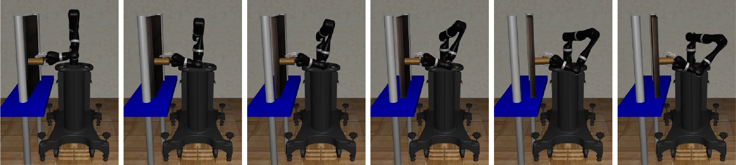
Figure 3: Regularly-timed stills of a single rollout of VICES (top) and RMP-VICES (bottom) after training is complete.

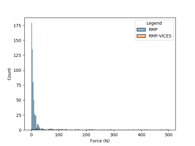
(a) Door-open.

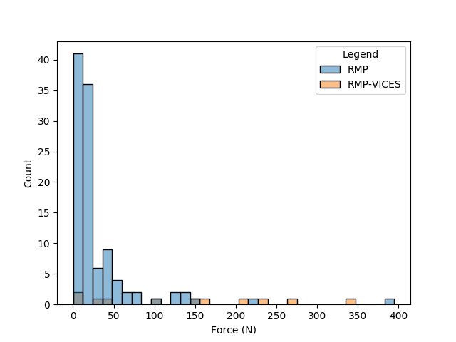
(b) Block-push.

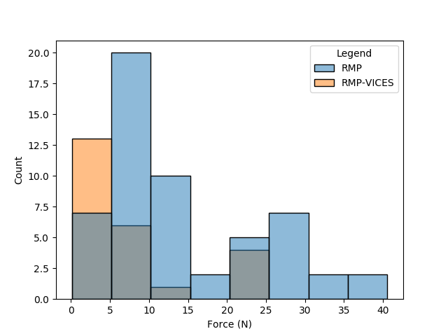
(c) Traj-follow.

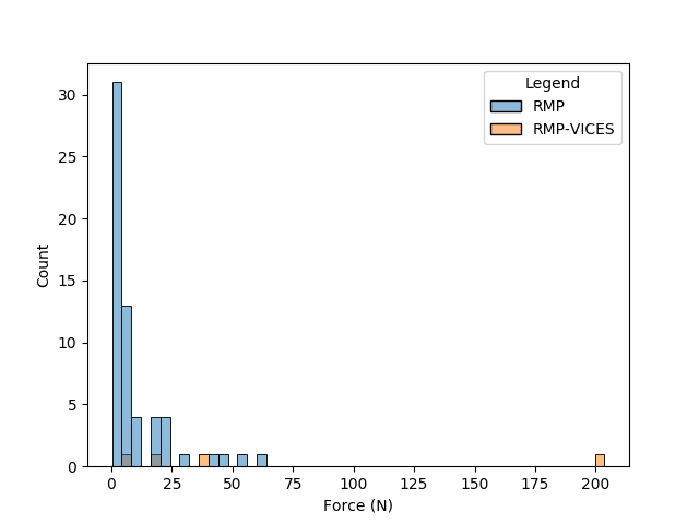
(d) Door-open.

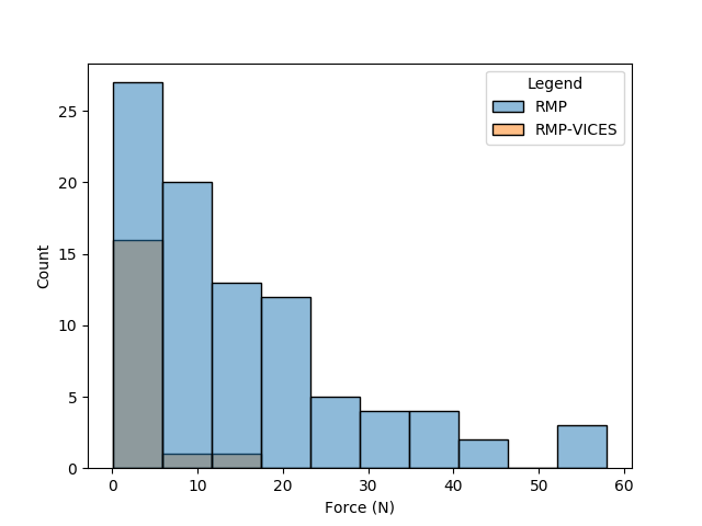
(e) Block-push.

Figure 4: Severity of collision events in training (a,b), and in environments with randomly generated obstacles (c-e).

V Results

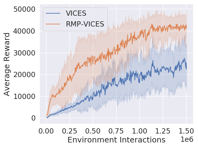
(a) Traj-follow., performance

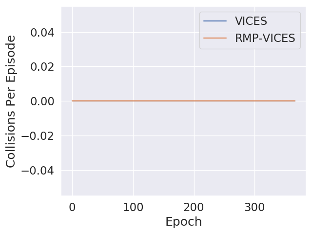
(b) Trajectory-follow., collisions

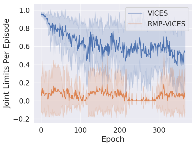
(c) Trajectory-follow., joint limits

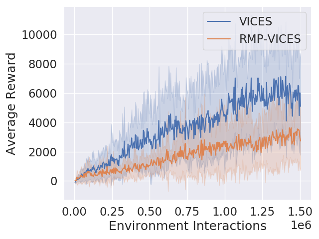
(d) Door-opening, performance

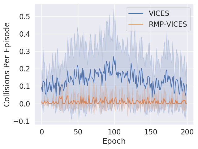
(e) Door-opening, collisions

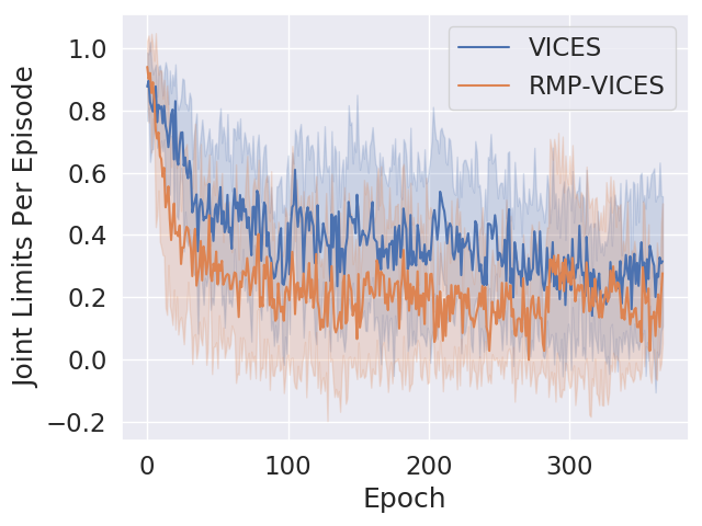
(f) Door-opening, joint limits

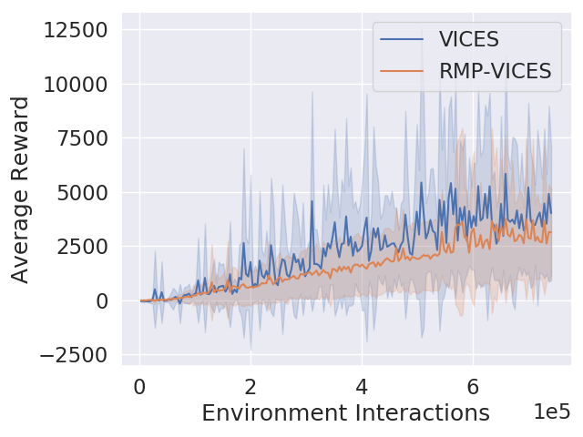
(g) Block-pushing, performance

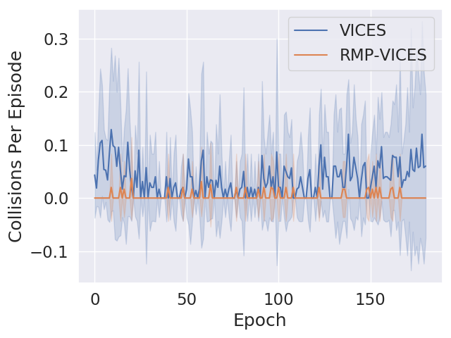
(h) Block-pushing, collisions

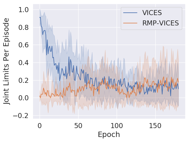
(i) Block-pushing, joint limits

Figure 5: Average reward, collision, and joint limit performance of VICES and RMP-VICES over the course of training on the trajectory-following (5(a),5(b),5(c)), door-opening (5(d),5(e),5(f)), and block-pushing domains (5(d),5(e),5(f)). When integrating the average curves for joint limits and collision avoidance behaviors, we see that RMP-VICES outperforms VICES in every domain. Percent decrease in collision and joint limit rates, respectively: trajectory-following: N/A%, 90.5%; door-opening: 39.8%, 90.7%; block-pushing: 54.6%, 93.2%.

V-A Safety During Training

In the trajectory-following task, RMP-VICES has far fewer joint-limit events than VICES (Fig. 5(c)) throughout training. Furthermore, RMP-VICES learns more sample-efficiently than just VICES alone (Fig. 5(a)). Since violating a joint limit causes episode termination, RMP-VICES has access to more viable data earlier in training, which accelerates the agent’s ability to learn the task.

In the door-opening task, we see that while RMP-VICES avoids collision better than VICES (figs. 5(e), 4(a)), the agent trained with RMP-VICES learns with worse overall performance (Fig. 5(d)). However, RMP-VICES is significantly safer in guiding the robot away from collision avoidance behavior. After reviewing several rollouts of each policy (Fig. 3), we see that the policy learns a behavior that keeps the robot’s pose largely the same with the elbow pointing straight up, which the RMP-VICES joint-limit and collision-avoidance policy represses. As a result, the RMP-VICES controller first pitches the elbow downward, and then opens the door. Since we give a dense reward that increases with door angle, the RMP-VICES agent obtained a lower average reward in VICES. However, the RMP-VICES policy is a safer behavior than the one learned by VICES alone, since the VICES behavior is prone to collision with the door (Fig. 3). This problem can be addressed with better tuning of the joint-limit policy or by learning the Riemannian metric [11].

In the block-pushing task, we see that RMP-VICES starts with better joint-limiting performance at the beginning of training figs. 5(h) 5(i). While VICES performs slightly better than RMP-VICES in efficacy of learning, RMP-VICES is much more performant in collision avoidance throughout training.

V-B Deployment in Environments with Generated Obstacles

For each experiment, we choose the best performing seeds from the VICES and RMP-VICES agent from each domain, and played through 100 episodes with randomly-generated spherical obstacles in the environment. The size and location of the bounding volumes used for each domain were chosen as areas where the arm would frequently pass through to the solve the task. Table I gives an aggregation of the performance of VICES and RMP-VICES from this set of experiments. See Fig. 1 in the for visualizations of all three environments for a single rollout instance.

Relative to performance in training, we see a drop in performance in all tasks. This makes intuitive sense because neither the VICES nor RMP-VICES policies experienced these obstacles before training. RMP-VICES, in all tasks, collides less frequently than VICES. While we do see a slight drop in performance in average reward, it is important to note that the success of the agent must be measured by its efficacy its ability to remain safe while completing the task.

	Task	Avg. Reward	Coll.	Jnt Lim.
VICES	Traj-follow.	$7864\pm 1.167\times 10^{4}$	56	44
	Door-open.	$1703\pm 1.948\times 10^{3}$	61	36
	Block-push.	$1755\pm 2.256\times 10^{3}$	93	0
RMP-VICES	Traj-follow.	$6847\pm 3.723\times 10^{3}$	25	22
	Door-open.	$1051\pm 6.96\times 10^{2}$	5	11
	Block-push.	$1740.\pm 8.54\times 10^{2}$	19	0

TABLE I: Results from rollouts with randomly-generated obstacles. As collision or passing a joint limit triggers the episode to end, the maximum number of collision and joint events for a single domain for a single agent is 100.

It is clear that the agent trained on RMP-VICES exploits the geometric prior given by the collision-avoidance RMPs for more safe behavior. An agent trained with VICES alone has no obvious way to incorporate this information, and the arm moves through the space blindly without adjusting its trajectory to avoid the new obstacles in its path.

Furthermore, we see that RMP-VICES reduces the impact of collision between the arm and its surrounding environment. Here, we see that RMP-VICES in these domains exhibits a sharper distribution about 0N (Fig. 4).

VI Conclusion

We have presented RMP-VICES, a geometry-aware operational-space controller for contact-rich manipulation. Our formulation synthesizes learned impedance control in $\mathsf{SE(3)}$ with predefined collision and joint limit avoidance behaviors, yielding a safer framework for reinforcement learning of manipulation skills. Our evaluation shows reduced frequency of collision and joint limit violation on the majority of tasks studied, especially early in learning. The main drawbacks of our proposed approach are the intensive tuning efforts required to weight leaf policies appropriately in the RMP-tree. Our framework also lacks Lyapunov or control barrier-certificates that guarantee stability or safety set invariance, respectively. Future work is warranted to investigate the design and tuning of provably safety behaviors and their interaction with policy optimization.

References

- [1] R. Martín-Martín, M. A. Lee, R. Gardner, S. Savarese, J. Bohg, and A. Garg, “Variable impedance control in end-effector space: An action space for reinforcement learning in contact-rich tasks,” in Proc. 2019 IEEE/RSJ International Conference on Intelligent Robots and Systems, 2019, pp. 1010–1017.
- [2] F. J. Abu-Dakka and M. Saveriano, “Variable impedance control and learning—a review,” Frontiers in Robotics and AI, p. 177, 2020.
- [3] N. D. Ratliff, J. Issac, D. Kappler, S. Birchfield, and D. Fox, “Riemannian motion policies,” arXiv preprint arXiv:1801.02854, 2018.
- [4] C.-A. Cheng, M. Mukadam, J. Issac, S. Birchfield, D. Fox, B. Boots, and N. Ratliff, “Rmpflow: A geometric framework for generation of multitask motion policies,” IEEE Transactions on Automation Science and Engineering, vol. 18, no. 3, pp. 968–987, 2021.
- [5] O. Khatib, “Inertial properties in robotic manipulation: An object-level framework,” The International Journal of Robotics Research, vol. 14, no. 1, pp. 19–36, 1995.
- [6] ——, “A unified approach for motion and force control of robot manipulators: The operational space formulation,” IEEE Journal on Robotics and Automation, vol. 3, no. 1, pp. 43–53, 1987.
- [7] J. Luh, M. Walker, and R. Paul, “Resolved-acceleration control of mechanical manipulators,” IEEE Transactions on Automatic Control, vol. 25, no. 3, pp. 468–474, 1980.
- [8] Y. Nakamura, H. Hanafusa, and T. Yoshikawa, “Task-priority based redundancy control of robot manipulators,” The International Journal of Robotics Research, vol. 6, no. 2, pp. 3–15, 1987.
- [9] L. Sentis and O. Khatib, “Synthesis of whole-body behaviors through hierarchical control of behavioral primitives,” International Journal of Humanoid Robotics, vol. 2, no. 04, pp. 505–518, 2005.
- [10] J. A. Coelho Jr and R. A. Grupen, “A control basis for learning multifingered grasps,” Journal of Robotic Systems, vol. 14, no. 7, pp. 545–557, 1997.
- [11] A. Li, C.-A. Cheng, M. A. Rana, M. Xie, K. Van Wyk, N. Ratliff, and B. Boots, “RMP2: A Structured Composable Policy Class for Robot Learning,” in Proc. Robotics: Science and Systems, Virtual, July 2021.
- [12] M. Mukadam, C.-A. Cheng, D. Fox, B. Boots, and N. Ratliff, “Riemannian motion policy fusion through learnable lyapunov function reshaping,” in Proc. Conference on Robot Learning, ser. Proc. Machine Learning Research, L. P. Kaelbling, D. Kragic, and K. Sugiura, Eds., vol. 100. PMLR, 30 Oct–01 Nov 2020, pp. 204–219.
- [13] M. A. Lee, C. Florensa, J. Tremblay, N. Ratliff, A. Garg, F. Ramos, and D. Fox, “Guided uncertainty-aware policy optimization: Combining learning and model-based strategies for sample-efficient policy learning,” in Proc. 2020 IEEE International Conference on Robotics and Automation, 2020, pp. 7505–7512.
- [14] A. Handa, K. Van Wyk, W. Yang, J. Liang, Y. W. Chao, Q. Wan, S. Birchfield, N. Ratliff, and D. Fox, “Dexpilot: Vision-based teleoperation of dexterous robotic hand-arm system,” in Proc. 2020 IEEE International Conference on Robotics and Automation, 2020, pp. 9164–9170.
- [15] D. Kappler, F. Meier, J. Issac, J. Mainprice, C. G. Cifuentes, M. Wüthrich, V. Berenz, S. Schaal, N. Ratliff, and J. Bohg, “Real-time perception meets reactive motion generation,” IEEE Robotics and Automation Letters, vol. 3, no. 3, pp. 1864–1871, 2018.
- [16] K. P. Wabersich and M. N. Zeilinger, “Linear model predictive safety certification for learning-based control,” in Proc. 2018 IEEE Conference on Decision and Control, 2018, pp. 7130–7135.
- [17] T. Wei and C. Liu, “Safe control algorithms using energy functions: A united framework, benchmark, and new directions,” in Proc. 2019 IEEE 58th Conference on Decision and Control, 2019, pp. 238–243.
- [18] R. Cheng, G. Orosz, R. M. Murray, and J. W. Burdick, “End-to-end safe reinforcement learning through barrier functions for safety-critical continuous control tasks,” in Proc. AAAI Conference on Artificial Intelligence, vol. 33, no. 01, 2019, pp. 3387–3395.
- [19] S. A. Khader, H. Yin, P. Falco, and D. Kragic, “Stability-guaranteed reinforcement learning for contact-rich manipulation,” IEEE Robotics and Automation Letters, vol. 6, no. 1, pp. 1–8, 2021.
- [20] Y. Chow, O. Nachum, E. Duenez-Guzman, and M. Ghavamzadeh, “A lyapunov-based approach to safe reinforcement learning,” in Advances in Neural Information Processing Systems, S. Bengio, H. Wallach, H. Larochelle, K. Grauman, N. Cesa-Bianchi, and R. Garnett, Eds., vol. 31. Curran Associates, Inc., 2018.
- [21] F. Berkenkamp, M. Turchetta, A. Schoellig, and A. Krause, “Safe model-based reinforcement learning with stability guarantees,” in Advances in Neural Information Processing Systems, I. Guyon, U. V. Luxburg, S. Bengio, H. Wallach, R. Fergus, S. Vishwanathan, and R. Garnett, Eds., vol. 30. Curran Associates, Inc., 2017.
- [22] A. Bylard, R. Bonalli, and M. Pavone, “Composable geometric motion policies using multi-task pullback bundle dynamical systems,” in Proc. 2021 IEEE International Conference on Robotics and Automation, 2021, pp. 7464–7470.
- [23] Y. Zhu, J. Wong, A. Mandlekar, and R. Martín-Martín, “robosuite: A modular simulation framework and benchmark for robot learning,” in arXiv preprint arXiv:2009.12293, 2020.
- [24] J. Achiam, “Spinning Up in Deep Reinforcement Learning,” 2018.