Exact Percolation Probability on the Square Lattice

Abstract

We present an algorithm to compute the exact probability $R_{n}(p)$ for a site percolation cluster to span an $n\times n$ square lattice at occupancy $p$. The algorithm has time and space complexity $O(\lambda^{n})$ with $\lambda\approx 2.6$. It allows us to compute $R_{n}(p)$ up to $n=24$. We use the data to compute estimates for the percolation threshold $p_{c}$ that are several orders of magnitude more precise than estimates based on Monte-Carlo simulations.

1 Introduction

Most of the work in percolation is intimately connected with computer simulations. Over the years, various algorithms have been developped [1]. Think of the Hoshen-Kopelman algorithm to identify clusters [2], the cluster growth algorithms [3, 4] or the cluster hull generating algorithm [5, 6, 7] to name but a few. Another example is the the invasion percolation algorithm, that works well independently of the spatial dimension [8] and even on hyperbolic lattices with their “infinite” dimension [9].

The microcanonical union-find algorithm by Newman and Ziff [10, 11] was a major improvement for Monte-Carolo simulations. It is not only exceedingly efficient, but also simple and beautiful.

In this contribution we will introduce an algorithm for the exact enumeration of percolating configurations in $2d$ lattices. We will discuss this algorithm for site percolation on the square lattice, but the method can easily be adapted to other $2d$ lattices.

Our motivation to devise such an algorithm and to run it is twofold. First, because we think that it is always good to have exact solutions, even for small systems. And second, because one can use the enumeration results to compute estimates for the percolation threshold $p_{c}$ that are more accurate than anything achievable with Monte Carlo simulations.

The latter is a recent trend in percolation. Exact estimators for small systems combined with careful extrapolations have lead to estimates for $p_{c}$ with unprecedented accuracy for many different lattices, see [12] and references therein.

0.569(13)	MC $78\times 78$	1963 [13]
0.590(10)	Series	1964 [14]
0.591(1)	MC $250\times 250$	1967 [15]
0.593(1)	MC $256\times 256$	1975 [16]
0.592 74(10)	TM $10\times\infty$	1985 [17]
0.592 745(2)	MC $2048\times 2048$	1986 [18]
0.592 746 21(13)	MC $128\times 128$	2000 [10]
0.592 746 21(33)	MC $1594\times 1594$	2003 [19]
0.592 746 03(9)	MC $2048\times 2048$	2007 [20]
0.592 745 98(4)	MC $2048\times 2048$	2008 [21]
0.592 746 05(3)	TM $16\times\infty$	2008 [22]
0.592 746 050 95(15)	TM $22\times 22$	2013 [23]
0.592 746 050 792 10(2)	TM $22\times\infty$	2015 [24]

Table 1: Some published estimates of the percolation threshold for site percolation on the square lattice. TM refers to transfer matrix algorithms, MC to Monte-Carlo methods. See [18] and [21] for more extensive lists. Or consult the always up to date WikipediA entry on percolation thresholds, maintained by Bob Ziff.

The situation for site percolation is depicted in Table 1. TM refers to transfer matrix methods as a label for enumerative, exact solutions of small systems combined with careful extrapolations. MC stands for Monte-Carlo results. As you can see, in 2008 TM took over MC. We will also use TM and add two more values to this Table.

The paper is organized in three sections plus conclusions and appendix. The first section defines the task and introduces the generating function. The second section comprises a detailed description of the algorithm, followed by a brief discussion of the results. In the third section we describe the computation of high precision values for the percolation threshold $p_{c}$. Sections two and three can be read independently. The appendix explains some of the combinatorics behind the algorithm.

2 The Number of Percolating Configurations

Our focus is on site percolation on the $n\times m$ square lattice, where percolation refers to spanning the $m$ direction. In particular we want to compute the number $A_{n,m}(k)$ of spanning configurations with $k$ sites occupied. These numbers are conveniently organized in terms of the generating function

$$F_{n,m}(z)\equiv\sum_{k=0}^{nm}A_{n,m}(k)\ z^{k}\,.$$ (1)

The spanning probability at occupancy $p$ is given by

$$R_{n,m}(p)=(1-p)^{nm}\,F_{n,m}\left(\frac{p}{1-p}\right)\,.$$ (2)

The numbers $A_{n,m}(k)$ can be computed by enumerating all $2^{nm}$ configurations. Enumerating only the hulls of the spanning clusters [6] reduces this complexity to $O(\numprint{1,7}^{nm})$, but even with this speedup, the maximum feasible system size is $8\times 8$ [25].

Obviously $A_{n,m}(k)=0$ for $k<m$. For $k=m$, the only spanning cluster is a straight line of length $m$,

$$A_{n,m}(m)=n\,.$$ (3a)

For $$k=m+1$$ the spanning cluster is either a straight line with one extra site which does not contribute to spanning, or it is a line with a kink:

$$A_{n,m}(m+1)=n\,{nm-m\choose 1}+2(n-1)(m-2)\qquad(m\geq 2)\,.$$ (3b)

For $$k=m+2$$ a spanning configuration is either a straight line with two free sites, a line with one kink and one free site or a line with two small or one large kink:

$$A_{n,m}(m+2)= n\,{nm-m\choose 2}+2(n-2)\left(\binom{m-2}{2}+(m-2)\right)$$

$$+2(n-1)\big{(}(nm-m-3)+(m-3)(nm-m-2)\big{)}$$ (3c)

$$+2(n-1)\binom{m-3}{2}\qquad\qquad(m\geq 3)\,.$$

The formulae for $k=m+3,m+4,\ldots$ can be derived using similar considerations, but they quickly get complicated and are not very illuminating. And of course we are here to have the computer do this work.

In the high density regime we focus on the number of empty sites. Obviously we need at least $n$ empty sites to prevent spanning,

$$A_{n,m}(nm-k)=\binom{nm}{mn-k}\qquad(k<n)$$ (4a)

$$n n\times m n-1 \mathcal{I}_{m}(n)$$ empty sites can block spanning only if they form a path that a king can take from the left column of an chess board to the right column in moves. Let denote the number of such paths. Then

$$A_{n,m}(nm-n)=\mathcal{I}_{m}(n)\,.$$ (4b)

This number of royal paths would be $m3^{n-1}$ if the king were allowed to step on rows above and below the board. If he cannot leave the board, the number of paths is given by a more intricate formula [26]. On a quadratic board, however, the number of paths can be expressed by the Motzkin numbers $M_{k}$ (29):

$$\mathcal{I}_{n}(n)=(n+2)3^{n-2}+2\sum_{k=0}^{n-3}(n-k-2)3^{n-k-3}M_{k}\,.$$ (5)

Equations (3) and(4) can be used as sanity check for the algorithm. Another sanity check is provided by a surprising parity property [27],

$$F_{n,m}(-1)=\sum_{\text{even $k$}}A_{n,m}(k)-\sum_{\text{odd $k$}}A_{n,m}(k)=(-1)^{s(n,m)}$$ (6a)

with

$$s(n,m)=\left\lfloor\frac{m}{2}\right\rfloor n+\left\lceil\frac{m}{2}\right\rceil\,.$$ (6b)

3 Algorithm

If you want to devise an efficient algorithm for a computational problem, you would be well advised to consult one of the approved design principles of the algorithms craft [28]. In our case the algorithmic paradigm of choice is dynamic programming. The idea of dynamic programming is to identify a collection of subproblems and tackling them one by one, smallest first, using the solutions of the small problems to help figure out larger ones until the original problem is solved.

3.1 Dynamic Programming and Transfer Matrix

In the present case, a natural set of subproblems is the computation of $F_{n,m}(z)$ for a given occupation pattern in the $m$th row. For $n=2$, for example, either the left site, the right site or both sites are occupied:

$$F_{2,m}(z)=F_{2,m}^{\includegraphics[width=7.00002pt]{leftfull}}(z)+F_{2,m}^{\includegraphics[width=7.00002pt]{rightfull}}(z)+F_{2,m}^{\includegraphics[width=7.00002pt]{bothfull}}\,.$$

An all empty row can not occur in spanning configurations. The $m$th row can only represent a spanning configuration if the $(m-1)$th row is either or , hence

$$F_{2,m}^{\includegraphics[width=7.00002pt]{leftfull}}(z)=z\,F_{2,m-1}^{\includegraphics[width=7.00002pt]{leftfull}}(z)+z\,F_{2,m-1}^{\includegraphics[width=7.00002pt]{bothfull}}(z)\,.$$

Complementing the equations for $F_{2,m}^{\includegraphics[width=7.00002pt]{rightfull}}(z)$ and $F_{2,m}^{\includegraphics[width=7.00002pt]{bothfull}}(z)$, we can write this as matrix-vector product

$$\begin{pmatrix}F_{2,m}^{\includegraphics[width=7.00002pt]{leftfull}}(z)\\[4.30554pt] F_{2,m}^{\includegraphics[width=7.00002pt]{rightfull}}(z)\\[4.30554pt] F_{2,m}^{\includegraphics[width=7.00002pt]{bothfull}}(z)\end{pmatrix}=\begin{pmatrix}z&0&z\\[4.30554pt] 0&z&z\\[4.30554pt] z^{2}&z^{2}&z^{2}\end{pmatrix}\begin{pmatrix}F_{2,m-1}^{\includegraphics[width=7.00002pt]{leftfull}}(z)\\[4.30554pt] F_{2,m-1}^{\includegraphics[width=7.00002pt]{rightfull}}(z)\\[4.30554pt] F_{2,m-1}^{\includegraphics[width=7.00002pt]{bothfull}}(z)\end{pmatrix}\,.$$ (7)

For general values of $n$ we can write

$$F_{n,m}^{\sigma}(z)=\sum_{\sigma^{\prime}}T_{\sigma,\sigma^{\prime}}(z)\,F^{\sigma^{\prime}}_{n,m-1}(z)\,,$$ (8)

where $\sigma$ and $\sigma^{\prime}$ denote possible configurations that can occur in a row of width $n$. Each $\sigma$ in row $m$ represents all compatible configurations in the $n\times m$ lattice “above” it. Appropriately we refer to $\sigma$ as signature of all these configurations.

The idea of the algorithm to compute $F_{n,1}^{\sigma}(z)$ for all signatures $\sigma$ and then use (8) to iteratively compute $F_{n,2}^{\sigma}(z)$, $F_{n,3}^{\sigma}(z)$, etc., thereby reducing the two-dimensional problem with complexity $O(2^{nm})$ to a sequence of $m$ one-dimenional problems of complexity $O(\lambda^{n})$ each.

This particular form of a dynamic programming algorithm is known as transfer matrix method. When transfer matrices were introduced into statistical physics by Kramers and Wannier in 1941 [29], they were meant as a tool for analytical rather than numerical computations. Their most famous application was Onsager’s solution of the two dimensional Ising model in 1944 [30]. With the advent of computers, transfer marices were quickly adopted for numerical computations, and already in 1980, they were considered “an old tool in statistical mechanics” [31]. Yet the idea to use transfer matrices to compute spanning probabilities in percolation emerged only recently, and not in statistical physics but in theoretical computer science. For their analysis of a two-player board game, Yang, Zhou and Li [23] developped a dynamic programming algorithm to compute numerically exact values of the spanning probability for a given value of the occupation probability $p$. We build on their ideas for the algorithm presented here.

3.2 Signatures

Signatures are the essential ingredients of the algorithm. How do we code them? And what is their number? Both questions can be answered by relating signatures to balanced strings of parentheses.

Occupied sites in a signature can belong to the same cluster. Either because they are neighbors within the signature or because they are connected through a path in the lattice beyond the signature. In any case the set of signature sites that belong to the same cluster has a unique left to right order. This allows us to encode cluster sites using left and right parentheses (Figure 1). We represent the leftmost site of a cluster by two left parentheses ((, the rightmost site by two right parentheses )) and any intermediate cluster site by )(. An occupied site that is not connected to any other site within the signature is represented by ().

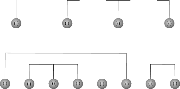
Figure 1: Coding table of cluster sites in a signature as parenthesis expressions (top) and example (bottom).

The resulting string is a balanced parentheses expression (with some white spaces from unoccupied sites), i.e., the total number of left parentheses equals the total number right parentheses, and counting from left to right, the number of right parentheses never exceeds the number of left parentheses. The latter is due to the topological constraints in two dimensions (two clusters can not cross). Identifying all sites of a cluster in a signature means matching parentheses in a balanced string of parentheses, a task that can obviously be accomplished in time $O(n)$.

Since we take into account only configurations that contain at least one spanning cluster, we need to identify clusters that are connected to the top row. We could follow [23] and use brackets [[, ]], ][ and [] to represent those clusters in a signature, thereby maintaining the concept of balanced strings of parentheses. It is more efficient, however, to use only a single symbol like $||$ for sites that are connected to the top. We can think of all $||$ sites being connected to each other by an all occupied zeroth row. Indentifying the left- and rightmost $||$ site in a signature can again be done in time $O(n)$.

The total number of signatures for spanning configurations depend on the width $n$ and the depth $m$. Some signatures can occur only in lattices of a minimum depth. The most extreme case in this respect are nested arcs, represented by signatures like

((  ␣  ((  ␣  $\cdots$   ␣  ))  ␣  )),

which can only occur if $m\geq\lceil n/2\rceil$. If $m$ is larger than this, however, the total number of signatures will only depend on $n$. In the Appendix we will prove that this number is given by

$$S_{n}=\sum_{r=0}^{\lfloor\frac{n-1}{2}\rfloor}{{n+1}\choose{2r+2}}{{2r+2}\choose r}\,\frac{3}{r+3}\equiv M_{n+1,2}\,,$$ (9)

where $M_{n+1,2}$ is the second column in the Motzkin triangle (34). The first terms of the series $S_{1},S_{2},\ldots$ are

$$1,3,9,25,69,189,518,1422,3915,10813,29964,83304,232323,649845,\ldots$$

We also show in the Appendix, that $S_{n}$ grows asymptotically as

$$S_{n}\sim\frac{\sqrt{3}\,3^{n+3}}{\sqrt{4\pi n^{3}}}\left(1-\frac{159}{16n}+\frac{36505}{512n^{2}}+O(\frac{1}{n^{3}})\right)\,.$$ (10)

3.3 From one dimension to zero dimensions

The central idea of the transfer matrix method (8) is to transform a two dimensional problem into a sequence of one dimensional problems, as a result of which the complexity reduces from $O(2^{nm})$ to $O(m2^{n}S_{n})$. This idea can be applied again. By building the new row site by site (Figure 2), we can subdivide the one dimensional problem into a sequence of $n$ zero dimensional problems. This reduces the complexity from $O(m2^{n}S_{n})$ to $O(nmS_{n})$.

Figure 2: Increasing the system size by adding a new site in the $(c+1)$th column of the partially filled row. The state of the new site may affect the cluster structure of the whole lattice, but we only need to update the signature, the cluster structure as it shows in the $n$ sites colored gray.

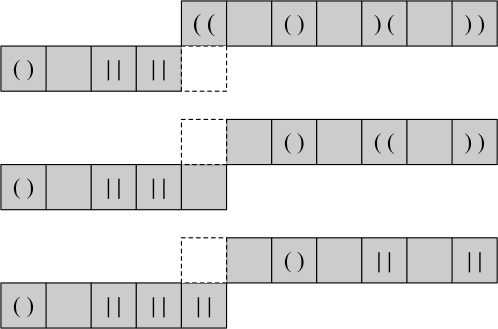
Figure 3: Signature of the cluster configuration of Fig 2 (top), and signatures after adding a new site that is either empty (middle) or occupied (bottom).

In this approach, the new row is partially filled up to column $c$. The corresponding signatures contain a kink at column $c$. Each signature is mapped to two signatures, depending on whether the added site at columns $c+1$ is empty or occupied (Figure 2).

The number of signatures $S_{n,c}$ depends on $n$ and $c$. We can think of a partially filled row as a full row of width $n+1$, where an extra site has been inserted between positions $c$ and $c+1$, this extra site being empty in all signatures. This gets us

$$S_{n}\leq S_{n,c}\leq S_{n+1}\,,$$ (11)

where the first inequality reflects the fact that the site at position $c$ has only two neighbors (left and up), and therefore less restrictions to take on “legal” values. The actual value of $S_{n,c}$ depends on $c$, see Table 2.

	1	2	3	4	5	6	7	8
1	$1$
2	4	3
3	12	11	9
4	33	31	31	25
5	91	85	87	85	69
6	249	233	237	237	233	189
7	683	638	651	646	651	638	518
8	1877	1751	1788	1777	1778	1787	1752	1422

Table 2: Values of $S_{n,c}$.

3.4 Condensation

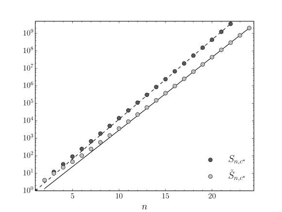
Figure 4: Number of signatures $S_{n,c^{\star}}$ (plain) and $\tilde{S}_{n,c^{\star}}$ (condensed). The lines are $S_{n,c^{\star}}\simeq\numprint{0.350}\cdot\numprint{2.85}^{n}$ and $\tilde{S}_{n,c^{\star}}\simeq\numprint{0.196}\cdot\numprint{2.61}^{n}$.

The number of signatures is paramount for the complexity of the algorithm. Let $S_{n,c^{\star}}\equiv\max_{c}S_{n,c}$. Figure 4 shows that $S_{n,c^{\star}}\simeq\numprint{0.350}\cdot\numprint{2.85}^{n}$. In particular, $S_{n,c^{\star}}$ exceeds the “Giga” threshold ($10^{9}$) for $n>20$. This is significant because we need to store pairs $(\sigma,F^{\sigma})$ for all signatures. For $S_{n,c^{\star}}$ above $10^{9}$, this means hundreds of GBytes of RAM. In this regime, space (memory) rather than time will become the bottleneck of our algorithm.

It turns out, however, that we can reduce the number of signatures. Consider a signature in row $m$ that contains the pattern $\ldots\mbox{\kern 0.59998pt\vrule height=2.15277pt}\vbox{\hrule width=6.00006pt}\hbox{\vrule height=2.15277pt}\,\mbox{()}\,\mbox{\kern 0.59998pt\vrule height=2.15277pt}\vbox{\hrule width=6.00006pt}\hbox{\vrule height=2.15277pt}\ldots$. All signatures in row $m+1$ that are derived from it, do not depend on whether the single () is actually occupied. Hence we can identify all signatures $\sigma=\ldots\mbox{\kern 0.59998pt\vrule height=2.15277pt}\vbox{\hrule width=6.00006pt}\hbox{\vrule height=2.15277pt}\,\mbox{()}\,\mbox{\kern 0.59998pt\vrule height=2.15277pt}\vbox{\hrule width=6.00006pt}\hbox{\vrule height=2.15277pt}\ldots$ with signatures $\sigma^{\prime}=\ldots\mbox{\kern 0.59998pt\vrule height=2.15277pt}\vbox{\hrule width=6.00006pt}\hbox{\vrule height=2.15277pt}\,\mbox{\kern 0.59998pt\vrule height=2.15277pt}\vbox{\hrule width=6.00006pt}\hbox{\vrule height=2.15277pt}\,\mbox{\kern 0.59998pt\vrule height=2.15277pt}\vbox{\hrule width=6.00006pt}\hbox{\vrule height=2.15277pt}\ldots$ and store only one pair $(\sigma^{\prime},F^{\sigma}+F^{\sigma^{\prime}})$ instead of two pairs $(\sigma,F^{\sigma})$ and $(\sigma^{\prime},F^{\sigma^{\prime}})$. For the same reason, we can also identify $\ldots\mbox{\kern 0.59998pt\vrule height=2.15277pt}\vbox{\hrule width=6.00006pt}\hbox{\vrule height=2.15277pt}\;\mbox{((}\;\mbox{))}\;\mbox{\kern 0.59998pt\vrule height=2.15277pt}\vbox{\hrule width=6.00006pt}\hbox{\vrule height=2.15277pt}\ldots$ with $\ldots\mbox{\kern 0.59998pt\vrule height=2.15277pt}\vbox{\hrule width=6.00006pt}\hbox{\vrule height=2.15277pt}\;\mbox{\kern 0.59998pt\vrule height=2.15277pt}\vbox{\hrule width=6.00006pt}\hbox{\vrule height=2.15277pt}\;\mbox{\kern 0.59998pt\vrule height=2.15277pt}\vbox{\hrule width=6.00006pt}\hbox{\vrule height=2.15277pt}\;\mbox{\kern 0.59998pt\vrule height=2.15277pt}\vbox{\hrule width=6.00006pt}\hbox{\vrule height=2.15277pt}\ldots$ and $\ldots\mbox{\kern 0.59998pt\vrule height=2.15277pt}\vbox{\hrule width=6.00006pt}\hbox{\vrule height=2.15277pt}\;\mbox{((}\;\mbox{)(}\;\mbox{))}\;\mbox{\kern 0.59998pt\vrule height=2.15277pt}\vbox{\hrule width=6.00006pt}\hbox{\vrule height=2.15277pt}\ldots$ with $\ldots\mbox{\kern 0.59998pt\vrule height=2.15277pt}\vbox{\hrule width=6.00006pt}\hbox{\vrule height=2.15277pt}\;\mbox{((}\;\mbox{\kern 0.59998pt\vrule height=2.15277pt}\vbox{\hrule width=6.00006pt}\hbox{\vrule height=2.15277pt}\;\mbox{))}\;\mbox{\kern 0.59998pt\vrule height=2.15277pt}\vbox{\hrule width=6.00006pt}\hbox{\vrule height=2.15277pt}\ldots$ and store only one of each pair.

In addition, the symmetry of the problem allows us to identify each signature of a full row ($c=n$) with its mirror image.

Let $\tilde{S}_{n,c}$ denote the number of signatures that haven been condensed by these rules, and let $\tilde{S}_{n,c^{\star}}=\max_{c}\tilde{S}_{n,c}$. Figure 4 shows that $\tilde{S}_{n,c^{\star}}\simeq\numprint{0.196}\cdot\numprint{2.61}^{n}$. The number of condensed signatures exceeds the “Giga” threshold only for $n>23$.

3.5 Implementation

		upper
left			$||$	((	))	)(	()
			a	b	b
		()	$||$	((	))	)(	()
	$||$	$||$	$||$	$||$      b	↯	↯	$||$
		$||$ $||$	$||$ $||$	$||$ $||$c			$||$ $||$
	((	((	↯	((      b	()		((
		(( )(		(( )(d	(( ))	(( )(	(( )(
	))	))	))      a	))      b	))      b	))	))
		)( ))	$||$  $||$c	)( )(	)( ))d	)( )(d	)( )(
	)(	)(	↯	)(      b	))	)(	)(
		)( )(		)( )(d	)( ))	)( )(	)( )(
	()	()	()      a	()      b	()      b	()	()      b
		(( ))	$||$ $||$	(( )(	)( ))	)( )(	(( ))

Table 3: Extension rules of the transfer matrix algorithm. Each cell shows the resulting configuration if the added site is empty (top) or occupied (bottom). Some update rules are non-local: ^a$||$ may only be deleted, if there is at least one other $||$  elsewhere in the signature, ^bdeleting (( or )) means shortening of the corresponding cluster, ^cthe whole cluster has to be connected to the top, and ^dtwo clusters merge. Configurations with ↯ must never occur.

The elementary step of the transfer matrix algorithm is the addition of a new lattice site in a partially filled row (Figure 3). This is implemented in a subroutine $\textbf{extend}(\sigma,c)$ that takes a signature $\sigma$ and a column $c$ as input and returns a pair $\sigma_{0},\sigma_{1}$, where $\sigma_{0}$ ($\sigma_{1}$) follows from $\sigma$ by adding an empty (occupied) site in column $c$. The rules for these computations are depicted in Table 3. The signatures $\sigma_{0}$ and $\sigma_{1}$ are of course condensed before they are returned. The subroutine extend is then called from within a loop over rows and columns of the lattice (Figure 5).

$L_{\text{old}}:=\text{first row configurations}$ $L_{\text{new}}:=\text{empty list}$ for $r=1,\ldots,m$ do      for $c=1,\ldots,n$ do          while $L_{\text{old}}$ not empty do               take $(\sigma,F^{\sigma})$ out of $L_{\text{old}}$               $\sigma_{0},\sigma_{1}:=\textbf{extend}(\sigma,c)$               if $(\sigma_{0},\cdot)\not\in L_{\text{new}}$ then add $(\sigma_{0},F^{\sigma})$ to $L_{\text{new}}$               else replace $(\sigma_{0},F)$ in $L_{\text{new}}$ with $(\sigma_{0},F+F^{\sigma})$               end if               if $(\sigma_{1},\cdot)\not\in L_{\text{new}}$ then add $(\sigma_{0},zF^{\sigma})$ to $L_{\text{new}}$               else replace $(\sigma_{1},F)$ in $L_{\text{new}}$ with $(\sigma_{1},F+zF^{\sigma})$               end if          end while          swap names $L_{\text{old}}\leftrightarrow L_{\text{new}}$      end for end for $F_{n,m}:=\sum_{(\sigma,F^{\sigma})\in L_{\text{old}}}F^{\sigma}$

Figure 5: Transfer Matrix Loop.

The algorithm maintains two lists $L_{\text{old}}$ and $L_{\text{new}}$ of configurations, where a configuration consists of a signature $\sigma$ and the corresponding generating function $F^{\sigma}$. $L_{\text{old}}$ is initialized with the $2^{n}-1$ first row configurations, in which each occupied site is connected to the top row by definition. $L_{\text{new}}$ is initially empty.

A configuration $(\sigma,F^{\sigma})$ is removed from $L_{\text{old}}$ and $\sigma_{0},\sigma_{1}=\textbf{extend}(\sigma,c)$ is computed. Then the configurations $(\sigma_{0},F^{\sigma})$ and $(\sigma_{1},zF^{\sigma})$ are inserted into $L_{\text{new}}$. This is repeated until $L_{\text{old}}$ is empty. At this point, $L_{\text{old}}$ and $L_{\text{new}}$ swap their names, and the process can be iterated to add the next site to the lattice.

If the lattice has reached its final size $nm$, the total generating function is the sum over all $F^{\sigma}$ for $(\sigma,F^{\sigma})\in L_{\text{old}}$.

With its six symbols      , $||$, ((, )(, ))and (), a signature can be interpreted as a senary number with $n$ digits. For $n\leq 24$, this number always fits into a 64-bit integer. Since

$$2^{64}=\numprint{3520522010102100444244424}_{6}\,,$$ (12)

we can also represent signatures of size $n=25$ by 64-bit integers, provided we choose the senary representation wisely: $\mbox{)(}=4_{6}$ and $\mbox{))}=5_{6}$.

The lists $L$ maintained by the algorithm contain up to $\tilde{S}_{n,c^{\star}}$ configurations. An efficient data structure is mandatory. We take advantage of the fact that the signatures can be ordered according to their senary value. This allows us to use an ordered associative container like set or map from the standard C++ library. Those guarantee logarithmic complexity $O(\log\tilde{S}_{n,c^{\star}})$ for search, insert and delete operations[32]

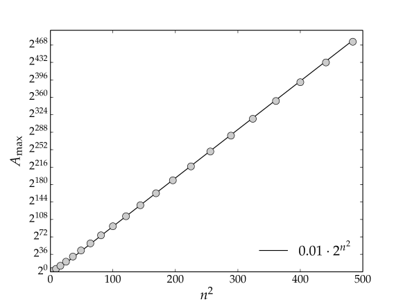
Figure 6: Maximum coefficient $A_{\mathrm{max}}(n)=\max_{k}A_{n,n}(k)$.

Equipped with a compact representation for the signatures and an efficient data structure for the list of configurations, we still face the challenge to store the large coefficients $A_{n,m}(k)$ of the generating functions $F_{n,m}^{\sigma}$. These numbers quickly get too large to fit within the standard fixed width integers with $32$, $64$ or $128$ bits (Figure 6).

One could use multiple precision libraries to deal with this problem, but it is much more efficient to stick with fixed width integers and use modular arithmetic: with $b$-bit integers, we compute $U^{(i)}_{n,m}(k)\equiv A_{n,m}(k)\bmod p_{i}$ for a set of prime moduli $p_{i}<2^{b}$ such that $\prod_{i}p_{i}>\max_{k}A_{n,m}(k)$ . We can then use the Chinese Remainder Theorem [32, 33] to recover $A_{n,m}(k)$ from the $U^{(i)}_{n,m}(k)$. This way we can trade space (bit size of numbers) for time (one run for each prime modulus).

3.6 Performance

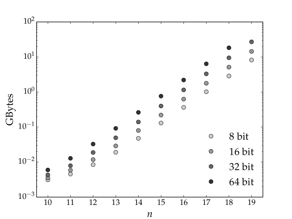
Figure 7: Memory required to compute $F_{n,n}$ with $b$-bit integers.

Figure 7 shows the actual memory consumption to compute $F_{n,n}$ with $b$-bit integers. Note that data structures like red-black-tress require extra data per stored element. Unfortunately the product of all primes below $2^{8}$ is not large enough to compute the coefficients in $F_{n,n}$ via modular arithmetic and the Chinese Remainder Theorem if $n\geq 19$. Hence 8-bit integers are essentially useless.

Extrapolation of the data in Figure 7 shows that the computation of $F_{n,n}$ for $n\leq 21$ cane be done with 16-bit integers on machines with 256 GB of RAM. Larger lattices require 384 GB ($n=22$) or 1 TB ($n=23$).

There is an alternative approach to determine $F_{n,m}$ with less memory. Instead of enumerating the coefficients $A_{n,m}(k)$, one can compute $F_{n,m}(z)$ for $nm$ integer arguments $z$ (again modulo a sufficient number of primes) and then use Lagrange interpolation to recover $F_{n,m}$. This approach requires only a single $b$-bit integer to be stored with each signature. The prize we pay is that now we need $nm$ computations, each consisting of several runs for a sufficient number of prime moduli. This was the approach we used to compute $F_{22,22}$ on $30\ldots 60$ machines with 256 GB each.

Yet another method suggests itself if one is mainly interested in evaluating the spanning probability $R_{n,m}(p)$ for a given value of $p$. Here we need to store only a single real number with each signature, and there is no need for multiple runs with different prime moduli. Quadruple precision floating point variables with 128 bit (__float128 in gcc) allow us to evaluate $R_{n,m}(p)$ with more than 30 decimals precision. We used this approach to compute $R_{n,n}(p)$ for $n=23,24$, see Table 4.

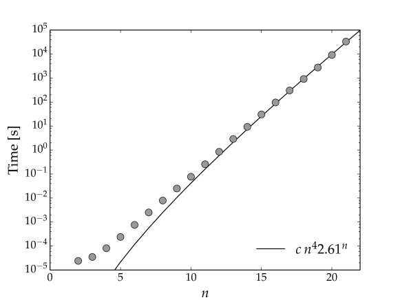
Figure 8: Time to evaluate $R_{n,n}(p)$ with 30 decimals accuracy on a laptop.

Figure 8 shows the time to evaluate $R_{n,n}(p)$ for given value $p$ and with 30 decimals accuracy, measured on a laptop. The time complexity corresponds to the expected complexity $O(n^{4}\tilde{S}_{n,c^{\star}})$. The $n^{2}$ iterations to build the lattice, combined with the $O(n)$ complexity of the subroutine extend and the $O(\log\tilde{S}_{n,c^{\star}})=O(n)$ complexity of the associative container set yield a scaling factor $n^{4}$. The number of signatures $\tilde{S}_{n,c^{\star}}\simeq\numprint{0.196}\cdot\numprint{2.61}^{n}$ then provide the exponential part of the time complexity.

Despite the exponential complexity, the algorithm is surprisingly fast for small values of $n$, even on a laptop. Systems up to $12\times 12$ can be computed in less than one second, $16\times 16$ takes 90 seconds. The largest system that fits in the 16 GByte memory of the author’s laptop is $21\times 21$. A single evaluation of $R_{21,21}(p)$ on the laptop takes about 9 hours.

3.7 Results

We have computed the generating functions $F_{n,m}(z)$ for $n\leq 22$ and all $m\leq n$. The data is available upon request. Here we will briefly discuss some properties of the coefficients $A_{n,m}(k)$. For simplicity we will confine ourselves to the quadratic case $m=n$.

$A_{nn}(k)$ has a maximum $A_{\text{max}}$ for $k=k_{\text{max}}(n)$. Our data reveals that

$$k_{\text{max}}(n)=\begin{cases}\frac{1}{2}n(n+1)&(n\leq 4)\\ \frac{1}{2}n(n+1)-1&(4<n\leq 22)\end{cases}$$ (13)

It is tempting to conjecture that $k_{\text{max}}(n)=\frac{1}{2}n(n+1)-O(\log n)$.

$A_{\text{max}}$ itself scales like $\simeq 2^{n^{2}}$ (Figure 6). This number determines how many prime moduli of fixed width we need to compute $A_{n,n}(k)$ via the Chinese Remainder Theorem.

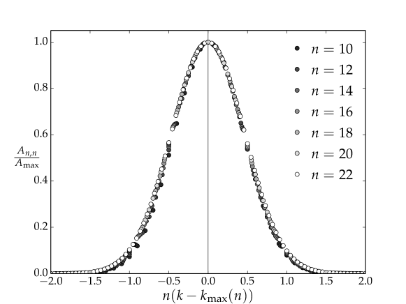
Figure 9: “Data collapse” in the number of spanning configurations.

The width of the maximum at $k_{\text{max}}$ scales like $n^{-1}$, as can be seen in the “data collapse” when plotting $\frac{A_{n,n}(k)}{A_{\text{max}}}$ versus $n(k-k_{\text{max}})$ (Figure 9).

4 Critical Density

The generating functions $F_{n,m}(z)$ can be analyzed in various ways. One can, for example, investigate their properties for arguments outside the “physical” interval $z\geq 0$. This is how the parity property (6) was discovered and then proven for a large, quite general class of lattices [27].

In this paper we use the generating function to compute finite size estimators for the critical density $p_{c}$ that we can then extrapolate to the infinite lattice.

4.1 Estimators

The properties of various finite-size threshold estimators for two-dimensional percolation have been discussed by Ziff and Newman [34]. Here we will focus on estimators $p_{\mathrm{med}}(n)$ and $p_{\mathrm{cell}}(n)$, defined as

$$R_{n,n}(p_{\mathrm{med}})=\frac{1}{2}$$ (14a)

and

$$R_{n,n}(p_{\mathrm{cell}})=R_{n-1,n-1}(p_{\mathrm{cell}})$$ (14b)

The values for these estimators up to $n_{\mathrm{max}}=24$ are shown in Table 4.

$n$	$p_{\mathrm{med}}(n)$	$p_{\mathrm{cell}}(n)$
1	0.500 000 000 000 000 000 000 000 000 000
2	0.541 196 100 146 196 984 399 723 205 366	0.618 033 988 749 894 848 204 586 834 365
3	0.559 296 316 001 323 534 755 763 920 789	0.620 734 471 730 213 489 279 430 523 252
4	0.569 724 133 968 027 153 228 040 518 353	0.619 583 777 217 655 117 827 765 082 346
5	0.575 810 073 211 627 653 605 032 974 314	0.613 506 053 696 798 307 677 288 581 191
6	0.579 702 757 132 443 521 419 439 978 330	0.609 208 761 667 991 711 639 989 601 974
7	0.582 351 295 080 082 980 073 474 691 830	0.606 075 989 265 451 882 260 569 905 672
8	0.584 241 466 489 847 673 860 351 132 398	0.603 762 879 768 292 280 370 335 551 749
9	0.585 641 556 861 396 511 416 995 666 354	0.602 011 983 338 557 157 018 606 681 442
10	0.586 710 034 053 406 359 804 690 473 124	0.600 656 365 889 941 520 514 281 630 459
11	0.587 545 601 376 707 076 865 096 376 747	0.599 585 402 842 798 543 263 268 780 420
12	0.588 212 470 606 443 263 171 973 079 741	0.598 724 257 102 302 868 949 743 766 602
13	0.588 753 953 651 382 767 097 855 532 073	0.598 021 063 882 979 665 779 438 359 439
14	0.589 200 171 193 723 644 344 640 059 478	0.597 439 041 437 080 848 283 968 950 089
15	0.589 572 624 709 616 129 448 171 107 692	0.596 951 544 750 954 799 494 938 258 995
16	0.589 887 013 723 258 987 069 435 195 722	0.596 538 896 774 607 564 321 149 432 769
17	0.590 155 029 961 590 857 817 809 334 101	0.596 186 311 743 107 211 382 955 497 774
18	0.590 385 533 260 670 477 887 261 817 585	0.595 882 504 071 658 438 851 295 137 696
19	0.590 585 341 987 611 428 265 706 601 016	0.595 618 737 176 226 408 186 670 067 141
20	0.590 759 776 378 574 624 089 782 736 423	0.595 388 160 640 890 684 818 467 256 078
21	0.590 913 039 569 092 174 937 740 096 798	0.595 185 340 192 645 002 572 869 419 257
22	0.591 048 489 639 675 518 303 675 880 577	0.595 005 919 018 756 026 574 538 302 404
23	0.591 168 837 021 863 732 985 091 670 808	0.594 846 370 109 520 325 790 777 710 845
24	0.591 276 289 864 951 685 617 852 112 360	0.594 703 812 696 743 490 456 949 711 289

Table 4: Finite size estimators for $p_{c}$ (14). All decimals are exact.

Both estimators are supposed to converge with the same leading exponent,

$$p_{\mathrm{med}}(n)-p_{c}\simeq c_{\mathrm{med}}\,n^{-1-1/\nu}\qquad p_{\mathrm{cell}}(n)-p_{c}\simeq c_{\mathrm{cell}}\,n^{-1-1/\nu}$$ (15)

with $\nu=\frac{4}{3}$. This scaling can clearly be seen in the data (Figure 10).

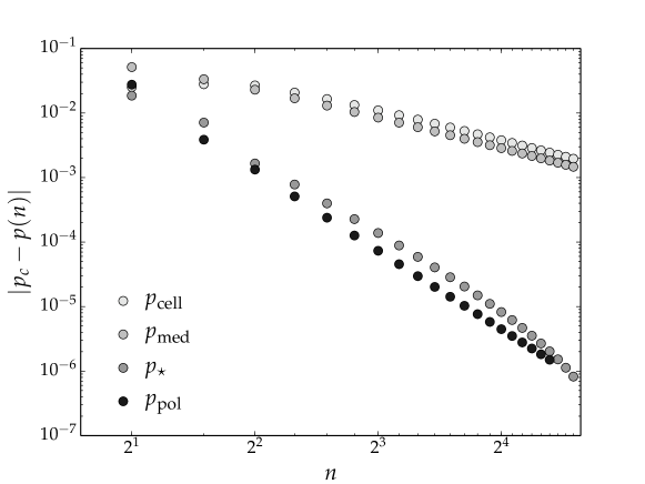
Figure 10: Finite size estimators for $p_{c}$ and their convergence.

Any convex combination of finite size estimators is another finite size estimator. We can choose $\lambda$ in $\lambda p_{\mathrm{med}}(n)+(1-\lambda)p_{\mathrm{cell}}(n)$ such that the leading order terms of $p_{\mathrm{med}}(n)$ and $p_{\mathrm{cell}}(n)$ cancel:

$$\lambda=\left(1-\frac{c_{\mathrm{med}}}{c_{\mathrm{cell}}}\right)^{-1}\,.$$ (16)

The precise values of $c_{\mathrm{med}}$ and $c_{\mathrm{cell}}$ are not known, but their ratio follows from scaling arguments [34]:

$$\frac{c_{\mathrm{med}}}{c_{\mathrm{cell}}}=-\frac{1}{\nu}=-\frac{3}{4}\,.$$ (17)

Hence we expect that the estimator

$$p_{\star}(n)\equiv\frac{4}{7}\,p_{\mathrm{med}}(n)+\frac{3}{7}\,p_{\mathrm{cell}}(n)$$ (18)

converges faster than both $p_{\mathrm{med}}(n)$ and $p_{\mathrm{cell}}(n)$. This is in fact the case, as can be seen in Figure 10.

Figure 10 also depicts the estimator $p_{\mathrm{pol}}(n)$, which is the root of a graph polynomial defined for percolation on the $n\times n$ torus [35, 36, 37]. Empirically, it converges like $\sim n^{-4}$ in leading order. Jacobsen [24] computed this estimator for $n\leq 21$ and extrapolated the results to obtain

$$p_{c}=\numprint{0.59274605079210}(2)\,.$$ (19)

This is the most precise value up to today. We have used it as reference $p_{c}$ in Figure 10 and we will continue to use it as reference in the rest of the paper.

4.2 Exponents

Extrapolation methods are commonly based on the assumption of a power law scaling

$$p(n)=p_{c}+\sum_{k=1}A_{k}n^{\Delta_{k}}$$ (20)

with exponents $0>\Delta_{1}>\Delta_{2}>\ldots$. These exponents can be determined by the following procedure.

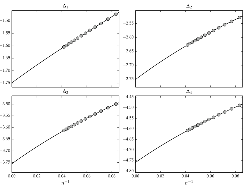
Figure 11: Exponent sequences $\Delta_{k}(n)$ of $p_{\mathrm{med}}(n)$ and 4th-order polynomial fits.

We start by considering the truncated form $p(n)=p_{c}+A_{1}n^{\Delta_{1}}$. From each triple of consecutive data points $p(n)$, $p(n-1)$ and $p(n-2)$ we can compute three unknows $p_{c}$, $A_{1}$ and $\Delta_{1}$. This gets us sequences $A_{1}(n)$ and $\Delta_{1}(n)$ that we can use to compute $\Delta_{1}=\lim_{n\to\infty}\Delta_{1}(n)$ and $A_{1}\equiv\lim_{n\to\infty}A_{1}(n)$. Figure 11 shows $\Delta_{1}(n)$ for $p(n)=p_{\mathrm{med}}(n)$ plotted versus $n^{-1}$ along with a 4th-order polynomial fit. The result $\Delta_{1}=-\frac{7}{4}$ is of course expected. It is stable under variations of the order of the fit and the number of low order data points excluded from the fit.

We then subtract the sequence $A_{1}n^{\Delta_{1}}$ from $p(n)$ to eliminate the leading scaling term $n^{\Delta_{1}}$. Considering again a truncated form $p(n)-A_{1}n^{\Delta_{1}}=A_{2}n^{\Delta_{2}}$, we can get sequences $A_{2}(n)$ and $\Delta_{2}(n)$ from three consecutive terms of this sequence. And again we extrapolate these sequences by fitting a low order polynomial in $n^{-1}$, thereby obtaining $\Delta_{2}$ and $A_{2}$.

Obviously, this can be iterated to determine the exponents $\Delta_{k}$ one by one, allthough the stability of the procedure deteriorates to some extent with each iteration. Figure 11 shows the extrapolations for $\Delta_{2}$, $\Delta_{3}$ and $\Delta_{4}$ for $p_{\mathrm{med}}$ with results

$$\Delta_{2}=-2.7516\approx-\frac{11}{4}\quad\Delta_{3}=-3.7553\approx-\frac{15}{4}\quad\Delta_{4}=-4.7590\approx-\frac{19}{4}$$ (21)

The results for $p_{\mathrm{cell}}$ are similar. These results provide compelling evidence that

$$\Delta_{k}=-\frac{4k+3}{4}\qquad(p_{\mathrm{med}},p_{\mathrm{cell}})\,.$$ (22)

These are the exponents that we will use in our extrapolations.

Applying the same procedure, Jacobsen [24] concluded that the scaling exponents for $p_{\mathrm{pol}}$ are

$$\Delta_{k}=-2k-2\qquad(p_{\mathrm{pol}})\,.$$ (23)

For $p_{\star}(n)$, we could not reliably compute exponents $\Delta_{k}$. It can already be sensed from the curvature in the logarithmic plot (Figure 10), that $p_{\star}(n)$ is not determined by a set of well separated exponents. This is the reason why we will not use $p_{\star}(n)$ for extrapolation in this contribution, despite its fast convergence.

4.3 Extrapolation

A study of extrapolation methods in statistical physics [38] demonstrated that Bulirsch-Stoer (BST) extrapolation [39] is a reliable, fast converging method. It is based on rational interpolation. For a given sequence of exponents $0<w_{1}<w_{2}<\ldots$ and $n$ data points $p(1),\ldots,p(n)$, one can compute coefficients $a_{0},\ldots,a_{N}$ and $b_{1},\ldots,b_{M}$ with $N+M+1=n$ such that the function

$$Q_{N,M}(h)=\frac{a_{0}+a_{1}h^{w_{1}}+a_{2}h^{w_{2}}+\cdots+a_{N}h^{w_{N}}}{1+b_{1}h^{w_{1}}+b_{2}h^{w_{2}}+\cdots+b_{M}h^{w_{M}}}$$ (24)

interpolates the data: $p(k)=Q_{N,M}(1/k)$ for $k=1,\ldots,n$. The value of $a_{0}$ yields the desired extrapolation $p(k\to\infty)$.

The best results are usually obtained with “balanced”  rationals $N=\lceil(n-1)/2\rceil$ and $M=\lfloor(n-1)/2\rfloor$. This is what we will use for our extrapolations.

The BST method discussed in [38] uses exponents $w_{k}=k\omega$, where the parameter $\omega$ is chosen to match the leading order of the finite size corrections. Here we choose $w_{k}=-\Delta_{k}=\frac{4k+3}{4}$.

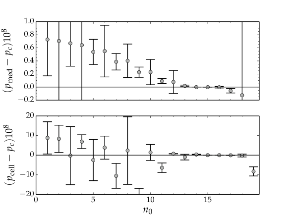
Figure 12: Rational extrapolation result vs. minimum system size $n_{0}$.

Having fixed the exponents and the degrees of nominator and denominator, we still have a free parameter: the number of data points to be included in the extrapolation. Since we are interested in the asymptotics $n\to\infty$ we will of course use the data of the large systems, but we may vary the size $n_{0}$ of the smallest system to be included. We expect that the extrapolation gets more accurate with increasing $n_{0}$, but only up to a certain point after which the quality deteriorates because we have to few data points left. This intuition is confirmed by the data (Figure 12).

The accuracy of an extropolation based on system sizes $n_{0},\ldots,n_{\mathrm{max}}$ is gauged by the difference between extrapolations of data points for $n_{0}+1,\ldots,n_{\mathrm{max}}$ and $n_{0},\ldots,n_{\mathrm{max}}-1$. These are the errorbars shown in Figure 12.

$n_{0}$	$p_{\mathrm{med}}$	$p_{\mathrm{cell}}$
13	0.592 746 050 98(12)	0.592 746 041(15)
14	0.592 746 050 788 5(22)⋆	0.592 746 054 1(16)
15	0.592 746 050 783(6)⋆	0.592 746 050 611(7)⋆
16	0.592 746 050 77(12)	0.592 746 050 59(16)⋆
17	0.592 746 050 23(34)	0.592 746 050 1(5)

Table 5: Extrapolations for different minimum system sizes $n_{0}$. Starred values are averaged to yield the final estimates (25) for $p_{c}$.

It seems reasonable to focus on the regime of $n_{0}$ where the results form a plateau with small errorbars, and to take the mean of these values as the final estimate of $p_{c}$. Using the values for $n_{0}=14,15$ ($p_{\mathrm{med}}$) and $n_{0}=15,16$ ($p_{\mathrm{cell}}$) (see Table 5) we get

$$p_{c} =\numprint{0.592746050786}(3)\qquad(p_{\mathrm{med}})\,,$$ (25a)

$$p_{c} =\numprint{0.59274605060}(8)\qquad(p_{\mathrm{cell}})\,.$$ (25b)

The first value deviates from the reference value (19) by 2 errorbars, the second by 2.5 errorbars.

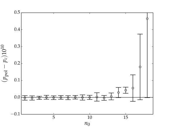
Figure 13: Rational extrapolation $p_{\mathrm{pol}}$ vs. minimum system size $n_{0}$.

The reference value $p_{c}$ 19 was obtained with different extrapolation approach. To see how consistent our method is, we applied it also to the estimator $p_{\mathrm{pol}}(n)$ from Jacobsen [24, Table. 2]. Here we used the exponents (23) in the BST extrapolation.

Figure 13 shows, that the errorbars are smaller than the errorbars on $p_{\mathrm{med}}$ and $p_{\mathrm{cell}}$ (note the scaling of the $y$-axis). The estimator $p_{\mathrm{pol}}$ is also more robust under variation of $n_{0}$. Taking the average of the estimates for $n_{0}=1,\ldots,10$ gives

$$p_{c}=\numprint{0.5927460507920}(4)\quad(p_{\mathrm{pol}})\,.$$ (26)

This value agrees with Jacobsen’s value (19) within the errorbars.

We believe that the superiority of the estimator $p_{\mathrm{pol}}$ is due to the better separation of scales: $\Delta_{k+1}-\Delta_{k}=-1$ for $p_{\mathrm{med}},p_{\mathrm{cell}}$ versus $\Delta_{k+1}-\Delta_{k}=-2$ for $p_{\mathrm{pol}}$.

5 Conclusions

We have introduced a transfer matrix algorithm to compute the generating function $F_{nm}(z)$ for the number of spanning configurations in an $n\times m$ square lattice. Adapting this algorithm to other $2d$ lattices and other boundary conditions (cylindrical, helical) is straightforward.

The exponential number of signatures imposes a hard limit on system sizes. With the current algorithm, computing $F_{25,25}(z)$ would require a computer with a 4 TB memory and a couple of months CPU time. Evaluating $R_{25,25}(p)$ for a single real argument $p$ requires 512 GB of memory und would take about one month.

We have also seen another example where the exact solution of small systems is sufficient to compute estimates for the critical density $p_{c}$ with an accuracy that no Monte-Carlo method could ever achieve. Or, as Bob Ziff put it, “Monte-Carlo is dead” [40] when it comes to computing $p_{c}$ for $2d$ systems.

This approach can be advanced. Not so much by solving larger systems, but by a better understanding of finite size estimators and their scaling.

Appendix A The Number of Signatures

To compute the number $S_{n}$ of signatures in fully completed rows, we use the connection of signatures and balanced strings of parentheses.

The number of balanced strings of parentheses length $2a$ is given by the Catalan number $C_{a}$ [41, Theorem 7.3],

$$C_{a}=\frac{1}{a+1}\,{2a\choose a}=\frac{(2a)!}{(a+1)!a!}=\prod_{k=2}^{a}\frac{a+k}{k}\,.$$ (27)

A completely balanced string of parantheses contains the same number $a$ of opening and closing parentheses. We will see that it is useful to consider also strings of parentheses that consist of $a$ opening parentheses and $b\leq a$ closing parentheses such that reading from left to right, every closing parenthesis matches an opening parenthesis. The number of these partially balanced strings of parentheses reads [42]

$$C_{a,b}=\frac{a-b+1}{a+1}{a+b\choose b}\qquad(a\geq b\geq 0)\,.$$ (28)

The numbers $C_{a,b}$ are known as Catalan’s triangle, and the Catalan numbers are the diagonal $C_{a}=C_{a,a,}$ of this triangle.

A.1 From Catalan to Motzkin numbers

In a signature, the parentheses are not independent. Occupied sites that are adjacent in a row belong to the same cluster. We deal with this local connectivity by considering runs of adjacent occupied sites as single entities that we may call h(orizontal)-clusters. A row of width $n$ contains at most $\lceil n/2\rceil$ h-clusters. Different h-clusters may be connected through previous rows, and again we have a unique left-right order and the topoligical constraints that allow us to identify h-clusters with strings of balanced parentheses expression, using the set of symbols ((, )), )( and (). Any legal signature with $r$ h-clusters corresponds to a balanced string of $2r$ parentheses and vice versa.

We write the occupation pattern of a row as $n$-bit word $s\in\{0,1\}^{n}$, where $0$ represents an empty site and $1$ represents an occupied site. Let $r(s)$ denote the number of h-clusters, i.e. runs of consecutive $1$s, in $s$. Then the number of signatures is

$$\sum_{s\in\{0,1\}^{n}}C_{r(s)}\,.$$

This sum can be simplified by computing the number of $n$-bit words with exactly $r$ h-clusters. For that we add a leading zero to the word. This ensures that every h-cluster has a zero to its left. The position of this zero and the position of the rightmost site of the h-cluster specify the h-cluster uniquely. Hence the number of $n$-bit words with $r$ h-clusters is given by ${{n+1}\choose{2r}}$, providing us with

$$\sum_{r=0}^{\left\lfloor\frac{n+1}{2}\right\rfloor}{{n+1}\choose{2r}}\,C_{r}\equiv M_{n+1}\,,$$ (29)

where $M_{n}$ is known as the $n$th Motzkin number [43, 44].

A.2 The spanning constraint

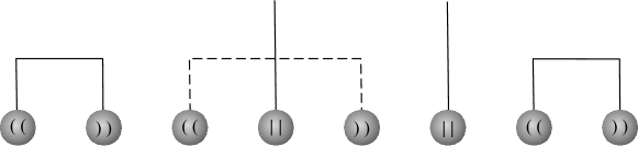
Figure 14: The dashed connection is forbidden: h-clusters can not connect across h-clusters that are connected to the top row.

Up to this point we have ignored that our signatures have an additional symbol $||$ for occupied sites connected to the top row. In a signature with $r$ h-clusters, any number $w\leq r$ of h-clusters can be connected to the top row:

$$S_{n}\leq\sum_{r=1}^{\left\lceil\frac{n}{2}\right\rceil}{{n+1}\choose{2r}}\,\sum_{w=1}^{r}{r\choose w}\,C_{r-w}\,.$$ (30)

This is only an upper bound because it does not take into account that h-clusters not connected to the top row can not be connected to each other across a top row h-cluster. In the example shown in Figure 14, the number of signatures compatible with the top row h-cluster is not $C_{6}=132$ but $C_{3}C_{1}C_{2}=10$.

We need to consider the compositions that $w$ top row h-clusters can impose upon the $r-w$ other h-clusters. The composition of an integer $n$ into $k$ parts is defined as an ordered arrangement of $k$ non-negative integers which sum to $n$ [45]. The compositions of $4$ into $2$ parts are

$$(0,4),(1,3),(2,2),(3,1),(4,0)\,.$$

A number of $w$ top row h-clusters can divide the $r-w$ other h-clusters into $w+1$ parts at most. This gets us

$$S_{n}=\sum_{r=1}^{\left\lceil\frac{n}{2}\right\rceil}{{n+1}\choose{2r}}\,\sum_{w=1}^{r}\sum_{\begin{subarray}{c}i_{k}\geq 0\\ i_{1}+\ldots+i_{w+1}=r-w\end{subarray}}C_{i_{1}}\cdots C_{i_{w+1}}\,.$$

Using Catalan’s convolution formula [46] for $1\leq k\leq n$,

$$\sum_{i_{1}+\ldots+i_{k}=n}C_{i_{1}-1}\cdots C_{i_{k}-1}=\frac{k}{2n-k}{{2n-k}\choose n}\qquad(1\leq k\leq n)\,,$$ (31)

we can write this as

$$S_{n}=\sum_{r=1}^{\left\lceil\frac{n}{2}\right\rceil}{{n+1}\choose{2r}}\,\sum_{w=1}^{r}\frac{w+1}{2r-w+1}{{2r-w+1}\choose{r+1}}\,.$$ (32)

The sum over $w$ can be done using binomial coefficient identities [47, Table 174]. The result reads

$$S_{n} =\sum_{r=1}^{\left\lceil\frac{n}{2}\right\rceil}{{n+1}\choose{2r}}\,\frac{3}{r+1}{{2r}\choose{r-1}}$$

$$=\sum_{r=1}^{\left\lceil\frac{n}{2}\right\rceil}{{n+1}\choose{2r}}\,C_{r+1,r-1}\,,$$ (33)

where (33) follows from (28) with $a=r+1$ and $b=r-1$. This result can be categorized by considering the generalization of (29). Analog to Catalan’s triangle, Motzkin’s triangle [48] is defined as

$$M_{n,k}=\sum_{r=0}^{\lfloor\frac{n-k}{2}\rfloor}{n\choose{2r+k}}\,C_{r+k,r}.$$ (34)

Hence $S_{n}=M_{n+1,2}$, the second column in Motzkin’s triangle. This sequence is number A005322 in the on-line encyclopedia of integer sequences.

A.3 Asymptotics

Allthough Motzkin’s triangle is a well known object in combinatorics, we could not find an explicit formula for the asymptotic scaling of $M_{n,2}$. Hence we compute it here, following the procedure outlined in [49].

Our starting point is the the generating function for $S_{n}=M_{n+1,2}$ [48]

$$F(x)=\sum_{n>0}S_{n}\,x^{n}=\frac{\left((1-x-\sqrt{(1+x)(1-3x)}\right)^{3}}{8x^{5}}\,.$$ (35)

The pole that determines the asymptotics of the coefficients is $x=1/3$. Expanding $F$ in terms of $\sqrt{1-3x}$ gives

$$F(x)=9-27\sqrt{3}\,(1-3x)^{\frac{1}{2}}+\frac{279}{2}(1-3x)-\frac{1485\sqrt{3}}{8}(1-3x)^{\frac{3}{2}}+\cdots\,.$$

The coefficients of the binonmial series that appear in this expansion are

$$\left[x^{n}\right](1-3x)^{\alpha} =(-3)^{n}{\alpha\choose n}=3^{n}{{n-\alpha-1}\choose n}$$ (36)

$$=3^{n}\frac{(-\alpha)(1-\alpha)\cdots(n-1-\alpha)}{n!}\,.$$

For $\alpha=0,1,2,3,\ldots$, the binomial series is finite and does not contribute to the asymptotic scaling. For $\alpha\neq 0,1,2,3,\ldots$, the binomial coefficient can be written as

$${{n-\alpha-1}\choose n}=\frac{\Gamma(n-\alpha)}{\Gamma(-\alpha)\Gamma(n+1)}\,,$$ (37)

and we can use the asymptotic series for the $\Gamma$ function

$$\frac{\Gamma(n-\alpha)}{\Gamma(n+1)}\sim n^{-\alpha}\left(\frac{1}{n}+\frac{\alpha(\alpha+1)}{2n^{2}}+\frac{\alpha(\alpha+1)(\alpha+2)(3\alpha+1)}{24n^{3}}\right.$$ (38)

$$\left.+\frac{\alpha^{2}(\alpha+1)^{2}(\alpha+2)(\alpha+3)}{48n^{4}}+O\left(\frac{1}{n^{5}}\right)\right)\,.$$

to obtain

$$\left[x^{n}\right]F(x)\sim\frac{\sqrt{3}\,3^{n+3}}{\sqrt{4\pi n^{3}}}\left(1-\frac{159}{16n}+\frac{36505}{512n^{2}}+O(\frac{1}{n^{3}})\right)$$ (39)

References

- [1] Ziff R M 2009 Efficient simulation in percolation lattices Complex Media and Percolation Theory Encyclopedia of Complexity and Systems Science Series ed Sahimi M and Hunt A G (New York: Springer-Verlag)
- [2] Hoshen J and Kopelman R 1976 Physical Review B 14 3438–3445
- [3] Leath P L 1976 Physical Review B 14 5046–5055
- [4] Alexandrowicz Z 1980 Physics Letters A 80 284–286
- [5] Grassberger P 1992 Journal of Physics A: Mathematical and General 25 5475–5484
- [6] Ziff R M 1992 Physical Review Letters 69 2670–2673
- [7] Ziff R M, Cummings P T and Stell G 1984 Journal of Physics A: Mathematical and General 17 3009–3017
- [8] Mertens S and Moore C 2018 Physical Review E 98 022120
- [9] Mertens S and Moore C 2018 Journal of Physics A: Mathematical and Theoretical 51 475001
- [10] Newman M E J and Ziff R M 2000 Physical Review Letters 85 4104–4107
- [11] Newman M E J and Ziff R M 2001 Physical Review E 64 016706
- [12] Scullard C R and Jacobsen J L 2020 Physical Review Research 2 012050(R)
- [13] Dean P 1963 Proceedings of the Cambridge Philosophical Society 59 397–410
- [14] Sykes M F and Essam J W 1964 Physical Review 133 A310–A315
- [15] Dean P and Bird N F 1967 Proceedings of the Cambridge Philosophical Society 63 477–479
- [16] Levinshteǐn M, Shklovskiǐ B, Shur M and Éfros A 1975 Zh. Eksp. Teor. Fiz. 69 386–392
- [17] Derrida B and Stauffer D 1985 Journal de Physique 46 1623–1630
- [18] Ziff R M and Sapoval B 1986 Journal of Physics A: Mathematical and General 19 L1169–1172
- [19] de Oliveira P, Nóbrega R and Stauffer D 2003 Brazilian Journal of Physics 33 616–618
- [20] Lee M 2007 Physical Review E 76 027702
- [21] Lee M 2008 Physical Review E 78 031131
- [22] Feng X, Deng Y and Blöte H W J 2008 Physical Review E 78 031136
- [23] Yang Y, Zhou S and Li Y 2013 Entertainment Computing 4 105–113
- [24] Jacobsen J L 2015 Journal of Physics A: Mathematical and Theoretical 48 454003
- [25] Klamser J U 2015 Exakte Enumeration von Perkolationssystemen Master’s thesis Otto-von-Guericke Universität Magdeburg
- [26] Yaqubi D, Ghouchan M F D and Zoeram H G 2016 Lattice paths inside a table I arXiv.org:1612.08697
- [27] Mertens S and Moore C 2019 Physical Review Letters 123 230605
- [28] Moore C and Mertens S 2011 The Nature of Computation (Oxford University Press) www.nature-of-computation.org
- [29] Kramers H A and Wannier G H 1941 Physical Review 60 252–262
- [30] Onsager L 1944 Physical Review 65 117–149
- [31] Derrida B and Vannimenus J 1980 Journale de Physique Lettres 41 L473–L476
- [32] Cormen T H, Leiserson C E and Rivest R L 1990 Introduction to Algorithms The MIT Electrical Engineering and Computer Science Series (Cambridge, Massachusetts: The MIT Press)
- [33] Knuth D E 1981 The Art of Computer Programming vol 2: Seminumerical Algorithms (Reading, Massachusetts: Addison-Wesley Publishing Company)
- [34] Ziff R M and Newman M E J 2002 Physical Review E 66 016129
- [35] Jacobsen J L and Scullard C R 2013 Journal of Physics A: Mathematical and Theoretical 46 075001
- [36] Jacobsen J L 2014 Journal of Physics A: Mathematical and Theoretical 47 135001
- [37] Mertens S and Ziff R M 2016 Physical Review E 94 062152
- [38] Henkel M and Schütz G 1988 Journal of Physics A: Mathematical and General 21 2617–2633
- [39] Bulirsch R and Stoer J 1964 Numerische Mathematik 6 413–427
- [40] Ziff R M 2021 Percolation on non-planar lattices Talk at the 34th M. Smoluchowski Symposium on Statistical Physics
- [41] Roman S 2015 An Introduction to Catalan Numbers Compact Textbooks in Mathematics (London: Birkhäuser)
- [42] Bailey D 1996 Mathematics Magazine 69 128–131
- [43] Motzkin T 1948 Bulletin of the American Mathematical Society 54 352–360
- [44] Oste R and der Jeugt J V 2015 The Electronic Journal of Combinatorics 22 P2.8
- [45] Heubach S and Mansour T 2009 Combinatorics of compositions and words. (Boca Raton, FL: CRC Press)
- [46] Regev A 2012 Integers 12 A29
- [47] Graham R L, Knuth D E and Patashnik O 1994 Concrete mathematics: a foundation for computer science 2nd ed (Addison-Wesley Publishing Company)
- [48] Donaghey R and Shapiro L W 1977 Journal of Combinatorial Theory (A) 23 291–301
- [49] Flajolet P and Sedgewick R 2009 Analytic Combinatorics (Cambridge University Press)