A posteriori error estimates via equilibrated stress reconstructions for contact problems approximated by Nitsche’s method
Abstract
We present an a posteriori error estimate based on equilibrated stress reconstructions for the finite element approximation of a unilateral contact problem with weak enforcement of the contact conditions. We start by proving a guaranteed upper bound for the dual norm of the residual. This norm is shown to control the natural energy norm up to a boundary term, which can be removed under a saturation assumption. The basic estimate is then refined to distinguish the different components of the error, and is used as a starting point to design an algorithm including adaptive stopping criteria for the nonlinear solver and automatic tuning of a regularization parameter. We then discuss an actual way of computing the stress reconstruction based on the Arnold–Falk–Winther finite elements. Finally, after briefly discussing the efficiency of our estimators, we showcase their performance on a panel of numerical tests.
Keywords: unilateral contact problem, weakly enforced contact conditions, a posteriori error estimate, equilibrated stress reconstruction, Arnold–Falk–Winther mixed finite element, adaptivity
MSC2020 classification: 74M15, 74S05, 65N15, 65N30, 65N50
1 Introduction
In various fields of solid mechanics and engineering it is essential to describe contact and friction between two bodies. This is the case, e.g., when modelling foundations and joints in buildings or when considering impact problems. In this paper, we focus on a simplified unilateral contact problem without friction, for which contact is mathematically expressed by some inequalities and complementarity conditions. These constraints translate non-penetration as well as the absence of cohesive forces and friction between the two bodies. In order to deal with the above constraints from a numerical point of view, different strategies have been proposed in the literature, including penalized formulations, mixed formulations, and weak enforcement à la Nitsche. We focus on the latter, which does not require the introduction of Lagrange multipliers and results in a coercive formulation that is easy to implement. The literature on the numerical approximation of contact problems is vast, and a comprehensive state-of-the-art lies outside of the scope of the present papers. We refer to the review articles [33, 9] and references therein for a broader discussion.
Nitsche’s method was originally introduced in [27] to weakly enforce Dirichlet boundary conditions. Its application to the unilateral contact problem considered in this paper was originally proposed in [11], where the well-posedness and convergence of a conforming finite element scheme are studied. Further extensions to problems involving friction or multiple bodies can be found in [12, 7, 29, 23]; we also mention [8] concerning the adaptation of these ideas to Hybrid High-Order discretizations [18, 17, 15]. A residual-based a posteriori error analysis can be found in [10] based on a saturation assumption.
In this paper we follow a different path and carry out an a posteriori error analysis based on equilibrated tractions in the spirit of the Prager–Synge equality [28] (see also [21] and [32, Chapter 7]). This approach, which does not require the saturation assumption when the dual norm of the residual is considered as an error measure, has also the advantage of avoiding unknown constants in the upper bound. The corresponding error estimate can additionally be refined in order to distinguish the various components of the error (discretization, linearization, regularization). This decomposition is leveraged here to design a fully adaptive resolution algorithm including an a posteriori-based stopping criterion for the nonlinear solver and the automatic tuning of the regularization parameter.
A crucial ingredient of our a posteriori analysis is a novel -conforming stress reconstruction obtained from the numerical solution by solving small problems on patches around mesh vertices. In the spirit of [30, 5], we use the Arnold–Falk–Winther mixed finite element spaces with weakly enforced symmetry [1]; strong symmetry could be enforced using the Arnold–Winther finite element spaces [2] as in [30], but would come at a significantly higher computational cost. The stress reconstruction is built so that its divergence and its normal component on the contact and Neumann portions of the domain boundary are locally in equilibrium with the volume and surface source terms, respectively (such equilibrium properties are not satisfied by stress fields resulting from -conforming finite element approximations). In order to distinguish the various error components, the stress reconstruction is additionally split so as to identify the contributions to the error resulting from linearization and regularization.
The main results of the paper are briefly summarized in what follows. The basic error estimate of Theorem 4 establishes a guaranteed upper bound for the dual norm of the residual. Such norm is shown in Theorem 7 to control the energy norm of the error up to a boundary term on the contact region (this term can be eliminated when a saturation assumption similar to the one used in [10] holds). A refined error estimate distinguishing the error components is derived in Theorem 11.
The rest of the paper is organized as follows. In Section 2 we describe the unilateral contact problem and its finite element approximation à la Nitsche. In Section 3 we derive a basic estimate for the dual norm of the residual and compare this norm with the energy norm. Section 4 contains a refined version of the estimate distinguishing the error components which serves as a starting point for the development of a fully adaptive algorithm. An equilibrated stress reconstruction based on the Arnold–Falk–Winther finite element is then proposed in Section 5. Section 6 briefly addresses the efficiency of the error estimators. Finally, some numerical results performed with the open source software FreeFem++ are presented in Section 7.
2 Setting
In this section we discuss the contact problem and its finite element discretization with weakly enforced contact conditions.
2.1 Unilateral contact problem
2.1.1 Strong formulation
Let and let be a connected open subset of representing an elastic body. We suppose that is a polygon (if ) or a polyhedron (if ), and that its boundary is partitioned into three non-overlapping parts , , and such that and ( denotes here the Hausdorff measure). In its reference configuration, the elastic body is in contact through with a rigid foundation, and we assume that the (unknown) contact zone in the deformed configuration will be included in . The body is clamped at and it is subjected to a volume force and to a surface load on ; see Figure 5 for an example.
Denoting by the unit normal vector on pointing out of , for any displacement field and for any density of surface forces defined on , we have the following (unique) decomposition into normal and tangential components:
| (2.1) |
We consider the following problem: Find the displacement field such that
| (2.2a) | ||||||
| (2.2b) | ||||||
| (2.2c) | ||||||
| (2.2d) | ||||||
| (2.2e) | ||||||
| (2.2f) | ||||||
where is the strain tensor field, is the Cauchy stress tensor, is the divergence operator acting row-wise on tensor valued functions, and is the fourth order symmetric elasticity tensor such that, for all second-order tensor , , with and denoting the Lamé parameters.
Remark 1 (Contact conditions).
The first contact condition (2.2e) is a complementarity condition: if, at a point , there is no contact in the deformed configuration (i.e., ), then the normal stress vanishes at that point (i.e., ); on the other hand, if at the normal stress is nonzero (i.e., ), then in the deformed configuration we still have contact in (i.e., ). These conditions also account for the absence of normal cohesive forces between the elastic body and the rigid foundation. The second contact condition (2.2f) simply establishes the absence of friction on .
The incorporation of standard friction models to the following a posteriori theory seems possible, but lies outside of the scope of the present paper. This subject will be addressed in future works.
2.1.2 Weak formulation
Let denote a measurable set of . In what follows, will be typically either equal to or to the union of a finite subset of mesh elements. We denote by , , the usual Sobolev space of index on , with the convention that , the space of square-integrable functions on . Its vector and tensor versions are denoted respectively by and . We let, similarly, and . Moreover, denotes the norm of or according to its argument. The first subscript is omitted when , i.e., is the standard norm of , , or according to its argument. The usual inner products of these spaces are denoted by , with the convention that the subscript is omitted when . In what follows, we will also need the space spanned by functions of with weak (row-wise) divergence in .
Denote by the subspace of incorporating the Dirichlet boundary condition on , and by its subset spanned by admissible displacements, i.e.,
The weak formulation of problem (2.2) corresponds to the following variational inequality (see, e.g., [24]): Find such that
| (2.3) |
where the bilinear form and the linear form are defined as follows: For all ,
| (2.4) |
Problem (2.3) admits a unique solution by the Stampacchia theorem.
2.2 Discretization
Let be a family of conforming triangulations of , indexed by the mesh size , where is the diameter of the element . This family is assumed to be regular in the classical sense; see, e.g., [13, Eq. (3.1.43)]. Furthermore, each triangulation is conformal to the subdivision of the boundary into , , and in the sense that the interior of a boundary edge (if ) or face (if ) cannot have non-empty intersection with more than one part of the subdivision. Mesh-related notations that will be used in the a posteriori error analysis are collected in Table 1. For the sake of simplicity, from this point on we adopt the three-dimensional terminology and speak of faces instead of edges also in dimension .
| Notation | Definition |
|---|---|
| Set of faces of | |
| Set of boundary faces, i.e., | |
| Partition of induced by the boundary and contact conditions | |
| Set of interior faces, i.e., | |
| Set of faces of the element , i.e., | |
| , | , |
| Set of all the vertices of | |
| Set of boundary vertices, i.e., | |
| Set of interior vertices, i.e., | |
| Set of vertices of the element , i.e., | |
| Set of vertices of the mesh face , i.e., | |
| Union of the elements sharing the vertex , i.e., |
For any mesh element or face, denotes the restriction to of -variate polynomials of total degree , and we set and . We seek the displacement in the standard Lagrange finite element space of degree with strongly enforced boundary condition on :
Denote by the projection on the half-line of negative real numbers , i.e., for all . For every real number and every positive bounded function , we define the following linear operator [9]:
| (2.5) |
where (notice that ). Assuming that , the first contact condition (2.2e) can be written as (see [14, 11]):
| (2.6) |
Remark 2 (Case ).
The linear operator is well defined on since it is a subspace of the space of broken polynomials. It can be easily extended to the space in the case , for which , as guarantees by the trace theorem.
From now on, will denote a fixed constant called Nitsche parameter, and we suppose that is the positive piecewise constant function on which satisfies: For all such that ,
We consider the following method à la Nitsche to approximate problem (2.2), originally introduced in [11]: Find such that
| (2.7) |
For the a priori analysis of the method, we refer to [11].
3 Basic a posteriori error estimate
In this section we derive a basic a posteriori error estimate based on the notion of equilibrated stress reconstruction.
3.1 Error measure
In the framework of a posteriori error estimation, the dual norm of a residual functional can be used as a measure of the error between the exact solution of the problem and the solution obtained with the finite element method. Denoting by the dual space of , for any the residual is defined by
| (3.1) |
where denotes the duality pairing between and . We equip with the following mesh-dependent norm:
| (3.2) |
where
| (3.3) |
It is easy to show that is subadditive and absolutely homogeneous, i.e., it is a seminorm. As a consequence, also is subadditive and absolutely homogeneous. Moreover, if we suppose , then both and are zero, and this implies by the Friedrichs inequality in , showing that is indeed a norm on .
The dual norm of the residual of a function on the normed space is given by
| (3.4) |
In what follows, the quantity will be used as a measure of the error committed approximating the exact solution with .
3.2 A posteriori error estimate
We start this section by introducing the concept of equilibrated stress reconstruction and the definition of five error estimators.
Definition 3 (Equilibrated stress reconstruction).
We will call equilibrated stress reconstruction any second-order tensor such that:
-
1.
,
-
2.
for every and every ,
-
3.
for every , and for every and every ,
-
4.
on .
Given an equilibrated stress reconstruction , for every element , we define the following local error estimators:
| (oscillation) | |||||
| (stress) | |||||
| (Neumann) | |||||
| (contact) |
Here, is the constant of the trace inequality with valid for every and ; see [32, Theorem 4.6.3] or [16, Section 1.4].
The estimator represents the residual of the force balance equation (2.2a) inside the element , the difference between the Cauchy stress tensor computed from the approximate solution and the equilibrated stress reconstruction, the residual of the Neumann boundary condition (2.2d), and the residual of the normal condition (2.2e) on the contact boundary.
Theorem 4 (A posteriori error estimate for the dual norm of the residual).
Proof.
Thanks to the regularity of and of its normal trace (see Properties 1. and 3. in Definition 3), the following Green formula holds:
| (3.5) |
where we have also used the decomposition (2.1) of the normal stress reconstruction into normal and tangential components on the contact boundary , and the fact that thanks to Property 4. in Definition 3. Now, fix such that and consider the argument of the supremum in the definition (3.4) of the dual norm of the residual. Expanding and according to their definition (2.4), adding and subtracting the term , using the symmetry of , and applying Green’s formula (3.5), we obtain
We estimate each term separately. Denoting by the -orthogonal projection onto , and using Property 2. of Definition 3 with test function , the Cauchy-Schwarz inequality, and the Poincaré inequality , the first term becomes
For the second term, we simply use the Cauchy-Schwarz inequality:
Denoting by the -orthogonal projection onto , and using Property 3. of Definition 3 with as a test function, the Cauchy-Schwarz inequality, and the trace inequality , , we have
where we recall that, for any , collects the Neumann faces of contained in . Finally, we consider the term on . We define, for all , the local counterpart of the seminorm (3.3)
where is the (possibly empty) set collecting the contact faces of contained in . Then, using the Cauchy-Schwarz inequality, we obtain
Let, for the sake of brevity, for any element . Combining the above results and applying the Cauchy-Schwarz inequality, we obtain
Remark 5 (A posteriori error estimate for stress reconstructions with contact friction).
3.3 Comparison between the residual dual norm and the energy norm
The goal of this section is to compare the dual norm with the energy norm of the error, where
| (3.6) |
Remark 6 (Coercivity of the bilinear form ).
The bilinear form on the space is elliptic with a constant which depends on the Lamé parameter and on the Korn constant :
| (3.7) |
Throughout the rest of this section, we adopt the following shorthand notation: For every , we write for with independent of the mesh size and of the Nitsche parameter .
Theorem 7 (Control of the energy norm).
Remark 8 (Role of the regularity assumption).
Proof of Theorem 7.
The proof adapts the ideas of [10, Theorem 3.5].
1) Proof of (3.8).
Let .
Using the definition (3.6) of the energy norm and the bilinearity of , we can write
| (3.11) |
For the term , we first use the definition (2.4) of the bilinear form followed by the symmetry of the Cauchy stress tensor to replace with , then an integration by parts, and, finally, the fact that satisfies (2.2) a.e. to infer:
| (3.12) |
Notice that, in the last term, only the normal component of the traction appears as on by (2.2f).
Concerning the term in (3.11), since solves (2.7) and , we have
| (3.13) |
where we have additionally expanded the linear form according to its definition (2.4).
Plugging (3.12) and (3.13) into (3.11), we then obtain
| (3.14) |
where, recalling the definition (3.1) of the residual,
Notice that the reformulation of in terms of the residual is a consequence of (3.1) and of the definition (2.4) of the linear form and of the bilinear form .
For the first term, we can write, by definition (3.4) of the dual norm,
| (3.15) |
We now want to show that for a properly selected function . From now on, we fix , where is the quasi-interpolation operator defined in [3, Eq. (4.11)], whose main properties are summarized in [10, Lemma 2.1]. We analyze separately the two parts composing the norm (see (3.2)). For the -seminorm, we use, in this order, the triangle inequality, the choice of , the boundedness in the -norm of the operator (i.e., for every ), and the ellipticity (3.7) of the bilinear form to write:
| (3.16) | ||||
Next, using the definition (3.3) of the seminorm , the choice of , and the ellipticity (3.7) of , we obtain:
| (3.17) |
where, to pass to the second line, we have used the following trace approximation property of (see [10, Lemma 2.1]): For all ,
with standing for the union of the mesh elements sharing at least one vertex with , see Figure 1. Recalling the definition (3.2) of the triple norm, squaring (3.16) and summing it to (3.17), and taking the square root of the resulting inequality, we conclude that
Combining this bound with (3.15), we obtain
| (3.18) |
We now consider the term . Using the Cauchy-Schwarz and trace inequalities, we have
| (3.19) |
Inserting (3.18) and (3.19) into (3.14), we obtain (3.8).
2) Proof of (3.10).
For the second part of the theorem, we work under the saturation assumption (3.9).
Using the contact condition (see (2.6)), and the definition (2.5) of the operator , we have
| (3.20) |
Due to the fact that and , it follows that
for every . Using the latter inequality with for the first term in (3.20) and the Cauchy-Schwarz inequality for the second one, we have
We continue using the generalized Young inequality for the second term followed by the saturation assumption (3.9) to write:
| (3.21) |
Combining (3.14), (3.18), and (3.21) we finally get, for a suitable real number ,
and, taking sufficiently large,
thus concluding the proof of (3.10). ∎
Theorem 9 (Control of the dual norm of the residual).
Proof.
1) Proof of (3.22). By definition (3.1) of the residual together with (2.2) (valid almost everywhere), and Green’s formula, it holds: For any ,
Then, using the symmetry of the Cauchy stress tensor , the Cauchy-Schwarz inequality, and the definition (3.2) of the norm , and additionally observing that
we have
By definition (3.4) of the dual norm, this yields (3.22).
2) Proof of (3.23).
Under the saturation assumption (3.9), starting from (3.22) and using (2.6),
we obtain, for all ,
where we have applied the property valid for any , with to pass to the second line and the triangle inequality to conclude. Then, using the saturation assumption (3.9) together with the ellipticity property (3.7) and the choice of , we obtain:
4 Identification of the error components
We consider the resolution of the (nonlinear) discrete problem (2.7) with an iterative method in which, at each iteration , the nonlinear term is replaced by a linear approximation . A new approximation of the discrete solution is then obtained solving the following problem: Find such that
| (4.1) |
The linearized operator is based on the following regularization of the projection : Given a real number (representing the amount of regularization),
Figure 2 shows the graphs of the projection operator and of the regularized operator . Notice that they coincide for and belongs to (but not to ). The linearized operator is obtained setting, for any ,
| (4.2) |
Here, we add the subscript to emphasize that the linear operator depends on the choice of this parameter. The refined error estimate presented in the following section enables an automatic tuning of .
4.1 A posteriori error estimate distinguishing the error components
We present in this section an error estimate for which enables one to identify and separate the different components of the error. The estimate hinges on the following assumption:
Assumption 10 (Decomposition of the stress reconstruction).
Let be an equilibrated stress reconstruction in the sense of Definition 3. Then, can be decomposed into three parts
| (4.3) |
where represents discretization, represents regularization, and represents linearization.
In Section 5 we will show how to obtain an equilibrated stress reconstruction which satisfies this assumption. Finally, we introduce the following local error estimators: For every element ,
| (oscillation) | (4.4a) | |||||
| (stress) | (4.4b) | |||||
| (regularization) | (4.4c) | |||||
| (linearization) | (4.4d) | |||||
| (Neumann) | (4.4e) | |||||
| (contact) | (4.4f) | |||||
The corresponding global error estimators are defined setting
| (4.5) |
Theorem 11 (A posteriori error estimate distinguishing the error components).
4.2 Fully adaptive algorithm
We propose an adaptive algorithm based on the error estimators (4.4) and (4.5), and on the result of Theorem 11. Denote by two user-dependent parameters that represent the relative magnitude of the regularization and linearization errors with respect to the total error. Moreover, we define the following local estimators:
The corresponding global counterparts are given by (4.5) with . With these estimators and the parameters , , we define stopping criteria for the regularization and linearization loops, respectively, so that both the parameter and the number of Newton iterations on every mesh refinement iteration will be fixed automatically by the adaptive algorithm. For all , the total error estimator is given by
| (4.8) |
5 Equilibrated stress reconstructions
We first show how to construct an equilibrated stress reconstruction that satisfies the conditions of Definition 3, then modify the construction to match Assumption 10.
5.1 Basic equilibrated stress reconstruction
Following the path of [5], we construct patchwise around the mesh vertices using Arnold–Falk–Winther mixed finite element spaces [1], which are based on a stress tensor constructed in the Brezzi–Douglas–Marini space (see, e.g., [6, Chapter 3] and [4, Chapter 2]), along with Lagrange multipliers that enforce a weak symmetry constraint. From this point on, will denote the set collecting all mesh vertices which lie on some Dirichlet boundary face. Notice that also contains the vertices lying at the intersection between and , .
For any element , and any integer , we set
At the global level, we define the following spaces
Notice that implies that its elements have continuous normal components across interfaces [15, Lemma 1.17]. Now, let , let be the solution of (2.7), and fix a mesh vertex . We denote by the patch around the node , see Figure 3, by the normal unit outward vector on its boundary and by the hat function associated with . On any patch we then define the following spaces:
| (5.1) | ||||
| (5.2) | ||||
Above, , , and denote the restrictions of the spaces , and to the subdomain , respectively. Moreover, is the space of normal traces on the patch boundary of elements in , i.e., it is the space of vector-valued broken polynomials of total degree on the set of boundary faces of the patch, while is space of rigid-body motions, i.e., and .
Remark 13 (Boundary condition for the reconstruction on internal vertices).
In the definition (5.1) of , we distinguish between boundary and internal vertices in order to ensure, in the case , zero normal components on the whole boundary of the patch even if .
Construction 14 (Basic equilibrated stress reconstruction).
Let, for any vertex , be the solution to the following problem:
| (5.3a) | ||||||
| (5.3b) | ||||||
| (5.3c) | ||||||
Extending by zero outside the patch , we set .
By definition of the space , a homogeneous Neumann boundary condition is enforced on the whole boundary of for interior vertices and on for boundary vertices. In particular, for boundary vertices in , a possibly non homogeneous Neumann boundary condition is enforced on the boundary faces of the patch. Therefore, when or , the right hand side of (5.3b) has to verify the following Neumann compatibility condition:
| (5.4) |
for any . Fixing a rigid-body motion , it is possible to check that (5.4) holds by taking as test function in (2.7). The following Lemma lists the main properties of the tensor resulting from Construction 14. In particular, it shows that satisfies all the conditions of Definition 3, i.e., it is an equilibrated stress reconstruction.
Lemma 15 (Properties of ).
Let be defined by Construction 14. Then, it holds
-
1.
;
-
2.
For every and every , ;
-
3.
For every and every , ;
-
4.
For every and every ,
Proof.
1) By definition, for any . Due to the no-flux boundary condition on internal faces enforced in the local problem on , the extension of by zero outside the patch is in and, as a consequence, .
2) First, we check that, for any , equation (5.3b) holds for every .
If , this is trivial since .
If, on the other hand, , it is sufficient to use the fact that (with orthogonal taken with respect to the -product) along with the Green formula, the definition (5.2) of , the Neumann compatibility condition (5.4), and (5.3c).
Now, fix and let . Extending by zero outside of , we have for all . Indeed, by definition, is composed by piecewise polynomials of degree at most that can be chosen independently inside each element of the patch. Summing (5.3b) over we obtain:
Here, we have used the fact that and over (so that, in particular, ).
3,4) We only detail the proof of 3) as that of 4) is similar.
Let and let be a polynomial defined on from the discrete normal trace space , i.e., a polynomial of total degree at most . Then, by the definition of (5.2),
5.2 Stress reconstruction distinguishing the error components
In Construction 14 we used the solution of the nonlinear problem (2.7) to reconstruct an equilibrated stress . However, as argued in Section 4, in practice we only dispose of an approximated solution obtained by means of a linearization method. Let be an integer and let be the solution of the linearized problem (4.1) with operator defined by (4.2). Then, for any boundary vertex , we set
and, for any internal vertex , (see (5.1)) for . Moreover, let be such that, for all ,
if , and if .
Construction 16 (Equilibrated stress reconstruction distinguishing the error components).
Let, for and any vertex , be the solution to the following problem:
where
Extending by zero outside the patch , we set , and we define .
By definition, and ensure that the forcing terms satisfy the following Neumann compatibility conditions for :
for any . The obtained tensor is an equilibrated stress reconstruction in the sense of Definition 3, and in particular it satisfies the properties stated by the following lemma whose proof is similar to that of Lemma 15 and is therefore omitted for the sake of conciseness.
Lemma 17 (Properties of ).
Let be defined by Construction 16. Then
-
1.
;
-
2.
For every and every , ;
-
3.
For every and every , ;
-
4.
For every and every ,
and
Remark 18 (Validity of Property 4. in Definition 3 and of Assumption 10).
The fourth property of the previous lemma implies that has the same direction as the normal vector , and, as a consequence, on , for . Moreover, by definition, is the sum of three tensors representing discretization, regularization and linearization, respectively. Therefore, is an equilibrated stress reconstruction in the sense of Definition 3 that additionally satisfies Assumption 10.
6 Efficiency of local estimators
In this section we briefly discuss the local efficiency of the estimators defined by (4.4) when using the stress reconstruction described in Section 5.2.
Following [31], for any we denote by the union of all elements sharing at least one vertex with (see Figure 4) and by the corresponding set of elements. Moreover, as in Subsection 3.3, stands for , where is a constant which is independent of the mesh size and of the Nitsche parameter . We introduce, for all , the local residual defined as follows: For all and all
where
Letting
with denoting the (possibly empty) set of faces of that lie on , the corresponding dual norm of the local residual for a function is
| (6.1) |
Theorem 20 (Local efficiency).
Remark 21 (Restriction on the space dimension).
Proof of Theorem 20.
The proof hinges on classical arguments, so we only briefly outline the main ideas and refer to [22, Section 5] for further details.
We introduce, for any element , a local residual-based estimator on the patch , following the path of [31], and then compare it with the local estimators (4.4) and the dual norm of the local residual operator (6.1). In particular, it is possible to prove the following two lemmas by adapting the approach of [20, Appendix A] and [5, Subsection 4.4], respectively:
Lemma 22 (Control of the residual-based estimator ).
For any element ,
| (6.3) |
Lemma 23 (Control of the local stress estimator).
Assume . Then, for every element ,
7 Numerical results
We present numerical cases to validate the a posteriori error estimate of Theorem 11 and show its use in the framework of an adaptive algorithm. The simulations are performed with the open source finite element library FreeFem++ (see [25] and also https://freefem.org/). We will use the notion of local and global total estimator: defined by (4.8) and
For the sake of brevity, above and throughout this section we omit the superscript which identifies the step of the Newton method.
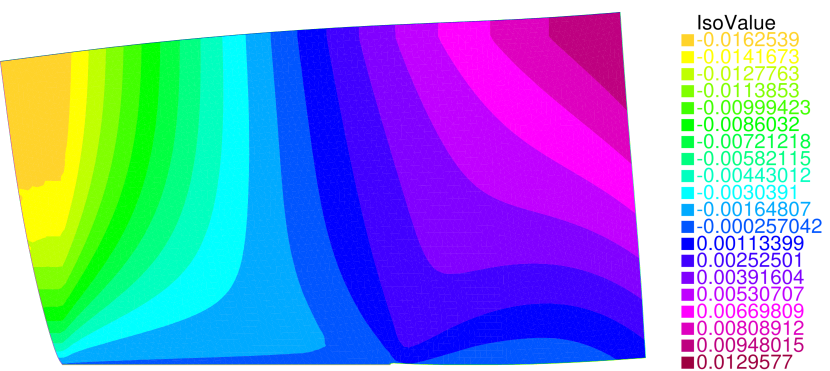
We consider a body that, in its reference configuration, occupies the rectangular domain (see Figure 5), with mechanical parameters and , corresponding to Lamé coefficients and . The body is subjected to a weight force . Homogeneous Dirichlet boundary conditions are enforced on , and the the body in its undeformed configuration is in contact with a rigid horizontal interface on . The Nitsche parameter is , whereas the regularization parameter which defines the operator is . A pressure acts on the right side of the body , and the rest of the boundary is free, i.e., on . Since a closed-form solution is not available for this configuration, we take as reference solution the function computed solving (2.7) with Lagrange finite elements on a fine mesh (). To compute the approximated solution , we use Lagrange elements (while this choice is known to lock in the quasi-incompressible limit, it is admissible for the set of parameters considered here and is compatible with the use of the lowest-order mixed finite elements available in FreeFem++ to compute the equilibrated stress reconstructions). In the deformed configuration, the body is in contact with the rigid foundation in a non-empty interval which is approximately . Figure 6(a) shows the vertical displacement in the deformed domain with an amplification factor equal to 5. Moreover, in Figure 6(b), which display the contact boundary part in the reference domain (black) and in the deformed domain (blue), we can easily identify the contact interval .
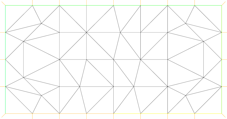
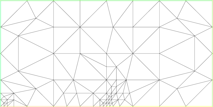
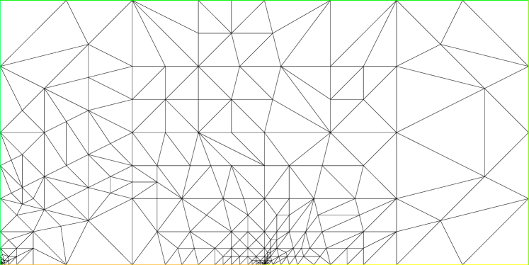
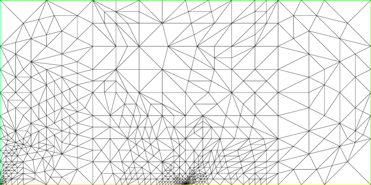
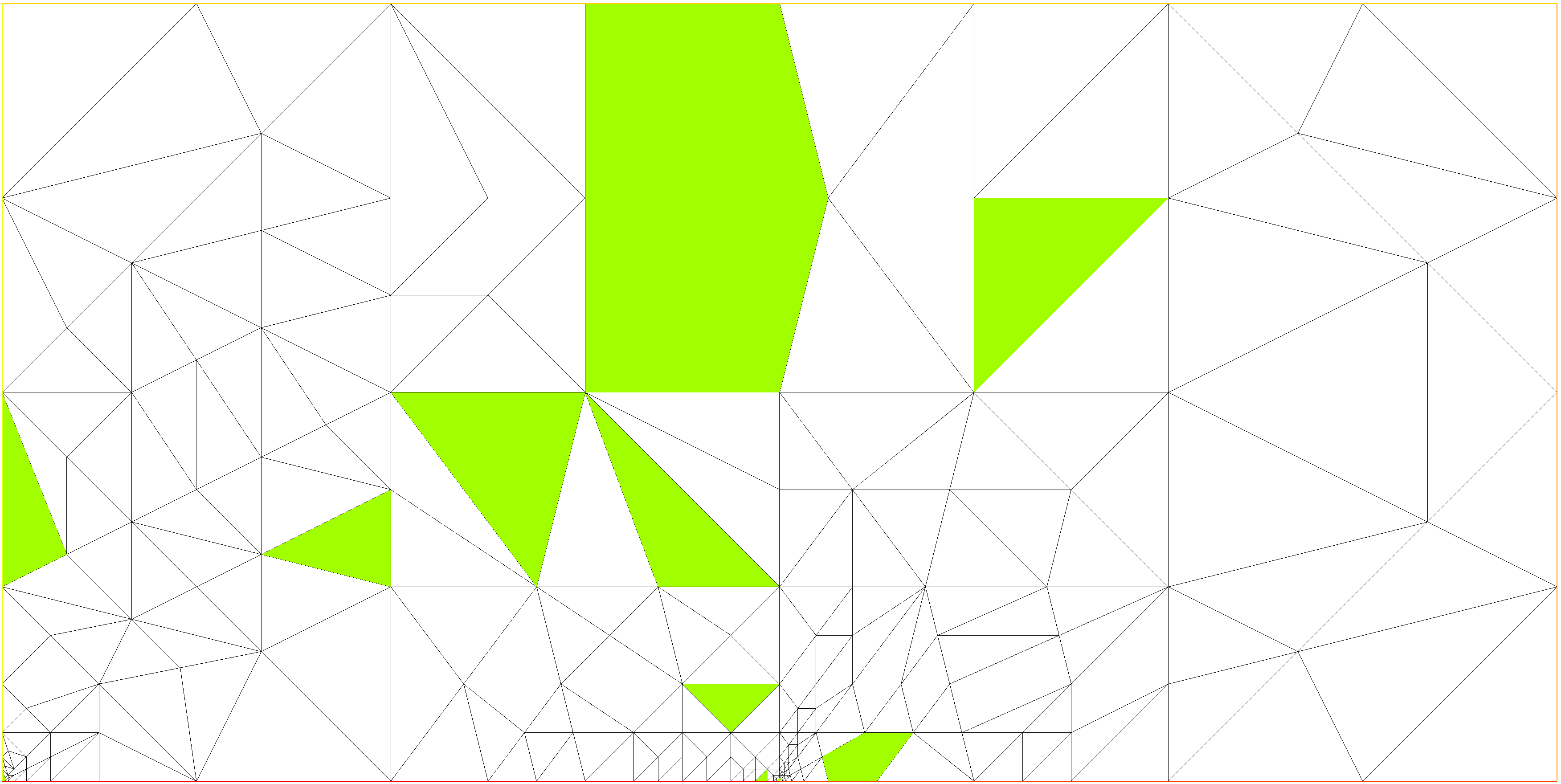
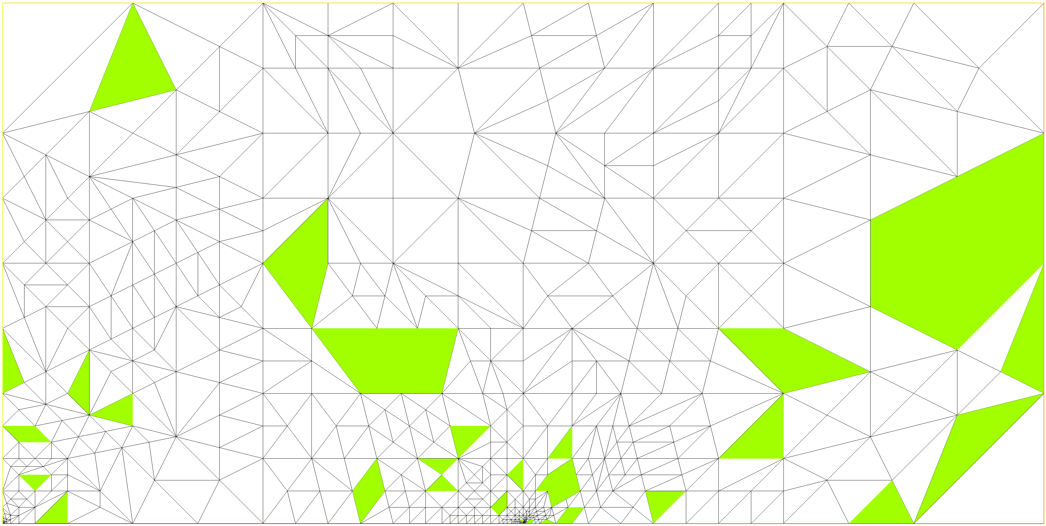
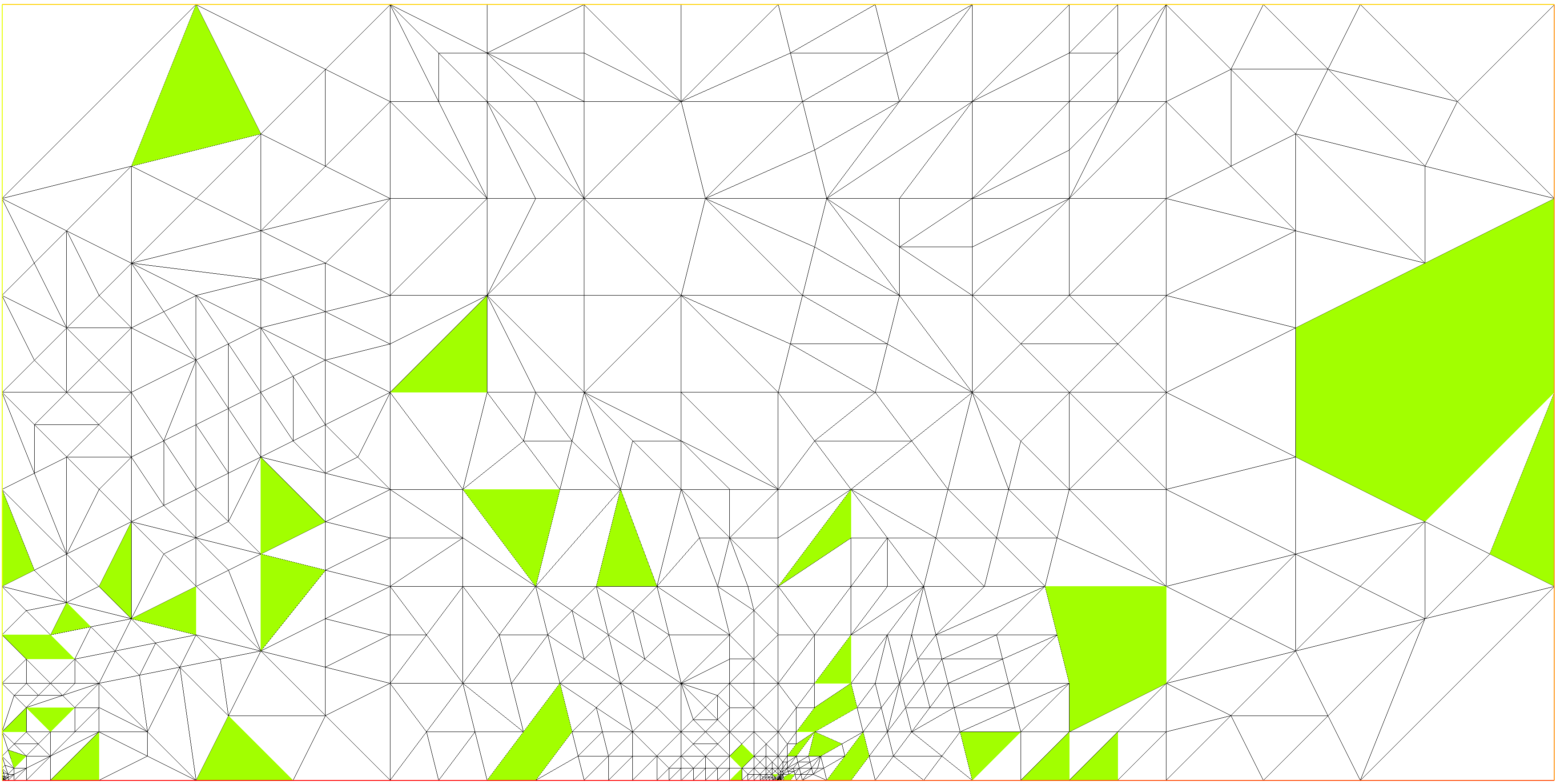
We refine adaptively the initial mesh following the distribution of the local total estimator , refining only the elements in which the value of this estimator is higher. In particular, at each refinement step, the 6% elements with larger estimated error are refined, i.e., are subdivided into four sub-triangles dividing each edge by two. Figure 7 shows the initial mesh and the result of adaptive refinement after 3, 7, and 11 steps, respectively. We remark that the refinement is concentrated on the endpoints of (singularities due to the homogeneous Dirichlet conditions) and near the contact interval . Figure 8(a) compares the convergence on uniformly and adaptively refined meshes for the -norm and for the energy norm , showing the corresponding curves as functions of the number of degrees of freedom. In particular, the uniform refinement is performed dividing all triangles of the mesh into four sub-triangles. The adaptive approach provides better convergence rates, i.e., adopting it we can achieve a fixed level of precision with fewer degrees of freedom. The asymptotic convergence rates are approximately 0.309 and 0.255 in the uniform case, and 0.450 and 0.449 in the adaptive case, for the -norm and energy norm, respectively (the optimal convergence rate for smooth solutions is ).
| Initial | 1st | 2nd | 3rd | 4th | 5th | 6th | 7th | 8th | 9th | 10th | 11th | |
|---|---|---|---|---|---|---|---|---|---|---|---|---|
| 7 | 0 | 1 | 0 | 0 | 0 | 0 | 0 | 0 | 0 | 0 | 0 | |
| 26 | 2 | 4 | 5 | 3 | 4 | 4 | 4 | 5 | 8 | 8 | 7 |
We recall that the measure of the error is the dual norm defined by (3.4), which is not computable (it can be, however, approximated through an elliptic lifting). As a consequence, recalling Theorems 7 and 9, we compare the global total estimator with the following quantities:
and
In particular, the latter incorporates an additional error component on the contact interface. Furthermore, we define the two following effectivity indices:
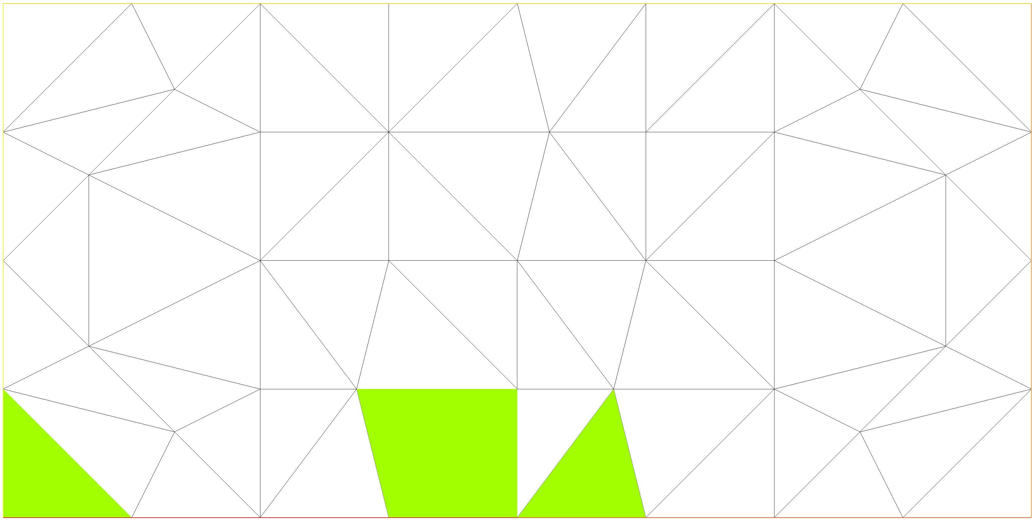
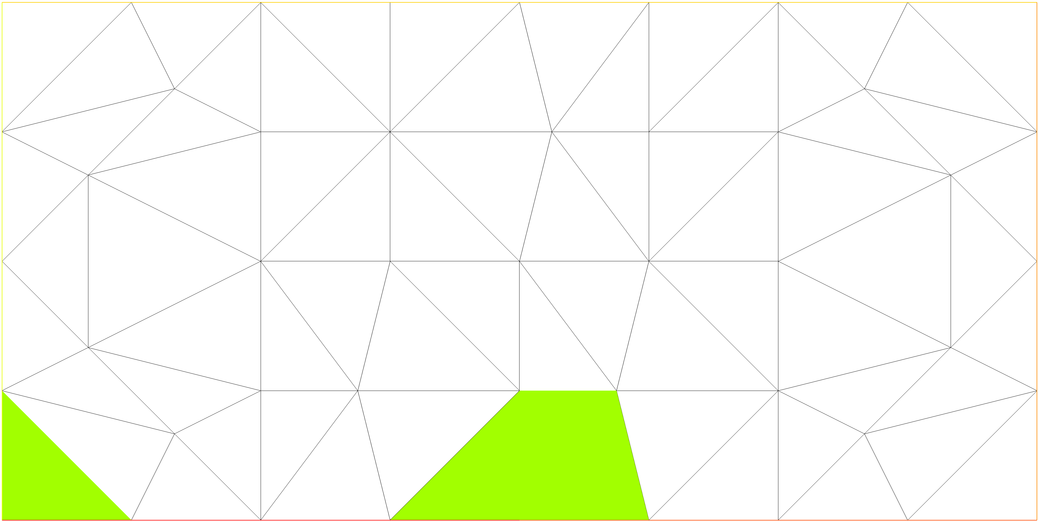
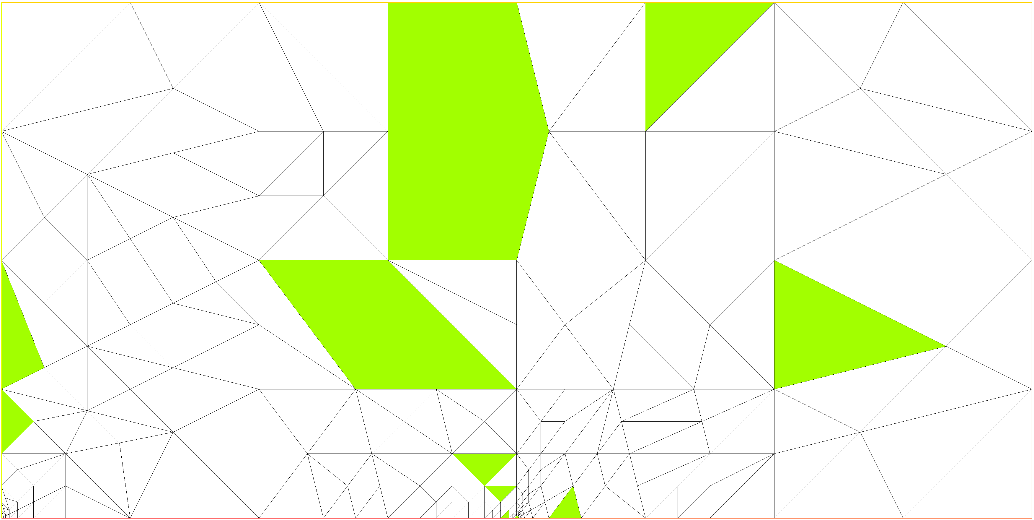
The results are illustrated in Figure 8(b) and 8(c). The total estimator always remains between the energy norm rescaled by a Lamé parameter and the upper bound for the dual residual norm , i.e., and . Figure 9 shows the distribution of the local total estimator at each mesh refinement step in both the uniform and adaptive frameworks. Here, we use boxplots to see where values concentrate. With the adaptive approach, all the local estimators are contained in an interval that becomes smaller and smaller at each refinement iteration, and the decrease of the maximum value is significantly faster than in the uniformly refined computation. Indeed, in the latter there is always a value which is much bigger than the others even if the number of degrees of freedom and the number of elements are high (in the last case, and ), showing that the error concentrates in specific areas. Figure 10 compares the selection of triangles to refine (highlighted in green) using the distribution of the energy norm (left) and the total estimator (right) for the initial mesh and the adaptively refined mesh after 6 and 10 steps. The sets of selected triangles are concentrated in the same zones.
Finally, we apply the fully adaptive Algorithm 1 with and . The initial regularization parameter is taken equal to the Young modulus and, at each step in which the global stopping criterion shown in Line 11 of Algorithm 1 is not satisfied, we divide it by 2. Table 2 contains the number of regularization and Newton iterations, denoted by and respectively, and Figure 11(a) displays the curves of the different global estimators for 11 adaptive refinement steps as functions of the degrees of freedom. The same estimators are shown in Figure 11(b) and 11(c) as functions of the Newton iterations for the 3rd and 9th adaptively refined meshes. A circle underlines the step (5th and 8th, respectively) at which the global stopping criterion of Line 9 is reached. At this step, the regularization estimator satisfies the global stopping criterion of Line 11, and the other ones have already stabilized.
Acknowledgements
This project has received funding from the European Union’s Horizon 2020 research and innovation program under grant agreement No 847593.
References
- [1] D. N. Arnold, R. S. Falk, and R. Winther, Mixed finite element methods for linear elasticity with weakly imposed symmetry, Mathematics of Computation, 76 (2007), pp. 1699–1723.
- [2] D. N. Arnold and R. Winther, Mixed finite elements for elasticity, Numerische Mathematik, 92 (2002), pp. 401–419.
- [3] C. Bernardi and V. Girault, A local regularization operator for triangular and quadrilateral finite elements, SIAM Journal of Numerical Analysis, 35 (1998), pp. 1893–1916.
- [4] D. Boffi, F. Brezzi, and M. Fortin, Mixed Finite Element Methods and Applications, vol. 44 of Springer Series in Computational Mathematics, Springer Science & Business Media, 2013.
- [5] M. Botti and R. Riedlbeck, Equilibrated stress tensor reconstruction and a posteriori error estimation for nonlinear elasticity, Computional Methods in Applied Mathematics, 20 (2020), pp. 39–59.
- [6] F. Brezzi and M. Fortin, Mixed and Hybrid Finite Element Methods, vol. 15 of Springer Series in Computational Mathematics, Springer-Verlag, 1991.
- [7] F. Chouly, An adaptation of Nitsche’s method to the Tresca friction problem, Journal of Mathematical Analysis and Applications, 411 (2014), pp. 329–339.
- [8] F. Chouly, A. Ern, and N. Pignet, A Hybrid High-Order discretization combined with Nitsche’s method for contact and Tresca friction in small strain elasticity, SIAM Journal on Scientific Computing, 42 (2020), pp. 2300–2324.
- [9] F. Chouly, M. Fabre, P. Hild, R. Mlika, J. Pousin, and Y. Renard, An overview of recent results on Nitsche’s method for contact problems, Geometrically Unfitted Finite Element Methods and Applications, 121 (2017), pp. 93–141.
- [10] F. Chouly, M. Fabre, P. Hild, J. Pousin, and Y. Renard, Residual-based a posteriori error estimation for contact problems approximated by Nitsche’s method, IMA Journal of Numerical Analysis, 38 (2018), pp. 921–954.
- [11] F. Chouly and P. Hild, A Nitsche-based method for unilateral contact problems: numerical analysis, SIAM Journal on Numerical Analysis, 51 (2013), pp. 1295–1307.
- [12] F. Chouly, P. Hild, and Y. Renard, Symmetric and non-symmetric variants of Nitsche’s method for contact problems in elasticity: theory and numerical experiments, Mathematics of Computation, 84 (2015), pp. 1089–1112.
- [13] P. G. Ciarlet, The finite element method for elliptic problems, vol. 40 of Classics in Applied Mathematics, Society for Industrial and Applied Mathematics (SIAM), Philadelphia, PA, 2002. Reprint of the 1978 original [North-Holland, Amsterdam; MR0520174 (58 #25001)].
- [14] A. Curnier and P. Alart, A generalized Newton method for contact problems with friction, Journal de Mécanique Théorique et Appliquée, 7 (1988), pp. 67–82.
- [15] D. A. Di Pietro and J. Droniou, The Hybrid High-Order method for polytopal meshes, vol. 19 of Modeling, Simulation and Application, Springer International Publishing, 2020.
- [16] D. A. Di Pietro and A. Ern, Mathematical aspects of discontinuous Galerkin methods, vol. 69 of Mathématiques & Applications (Berlin) [Mathematics & Applications], Springer, Heidelberg, 2012.
- [17] , A hybrid high-order locking-free method for linear elasticity on general meshes, Comput. Meth. Appl. Mech. Engrg., 283 (2015), pp. 1–21.
- [18] D. A. Di Pietro, A. Ern, and S. Lemaire, An arbitrary-order and compact-stencil discretization of diffusion on general meshes based on local reconstruction operators, Comput. Meth. Appl. Math., 14 (2014), pp. 461–472.
- [19] D. A. Di Pietro, M. Vohralík, and S. Yousef, Adaptive regularization, linearization, and discretization and a posteriori error control for the two-phase Stefan problem, Mathematics of Computation, 84 (2015), pp. 153–186.
- [20] L. El Alaoui, A. Ern, and M. Vohralík, Guaranteed and robust a posteriori error estimates and balancing discretization and linearization errors for monotone nonlinear problems, Computer Methods in Applied Mechanics and Engineering, 200 (2011), pp. 2782–2795.
- [21] A. Ern and M. Vohralík, Polynomial-degree-robust a posteriori estimates in a unified setting for conforming, nonconforming, discontinuous galerkin, and mixed discretizations, SIAM Journal on Numerical Analysis, 53 (2015), pp. 1058–1081.
- [22] I. Fontana, Modèles d’interface pour les ouvrages hydrauliques, PhD thesis, Université de Montpellier, École doctorale Information Structures Systèmes, In preparation, 2022.
- [23] T. Gustafsson, R. Stenberg, and J. Videman, On Nitsche’s method for elastic contact problems, SIAM Journal on Scientific Computing, 42 (2020), pp. B425–B446.
- [24] J. Haslinger, I. Hlaváček, and J. Nečas, Numerical methods for unilateral problems in solid mechanics, in Finite Element Methods (Part 2), Numerical Methods for Solids (Part2), vol. 4 of Handbook of Numerical Analysis, Elsevier, 1996, pp. 313–485.
- [25] F. Hecht, New development in FreeFem++, J. Numer. Math., 20 (2012), pp. 251–265.
- [26] P. Jiránek, Z. Strakoš, and M. Vohralík, A posteriori error estimates including algebraic error and stopping criteria for iterative solvers, SIAM Journal on Scientific Computing, 32 (2010), pp. 1567–1590.
- [27] J. Nitsche, Über ein variationsprinzip zur lösung von Dirichlet-problemen bei verwendung von teilräumen, die keinen randbedingungen unterworfen sind, Abhandlungen aus dem Mathematischen Seminar der Universität Hamburg, 36 (1971), pp. 9–15.
- [28] W. Prager and J. L. Synge, Approximations in elasticity based on the concept of function space, Quart. Appl. Math., 5 (1947), pp. 241–269.
- [29] Y. Renard, Generalized Newton’s methods for the approximation and resolution of frictional contact problems in elasticity, Computer Methods in Applied Mechanics and Engineering, 256 (2013), pp. 38–55.
- [30] R. Riedlbeck, D. A. Di Pietro, and A. Ern, Equilibrated stress tensor reconstructions for linear elasticity problems with application to a posteriori error analysis, in Finite Volumes for Complex Applications VIII - Methods and Theoretical Aspects, 2017, pp. 293–301.
- [31] R. Verfürth, A review of a posteriori error estimation techniques for elasticity problems, Computer Methods in Applied Mechanics and Engineering, 176 (1999), pp. 419–440.
- [32] M. Vohralík, A posteriori error estimates for efficiency and error control in numerical simulations, UPMC Sorbonne Universités, February 2015.
- [33] B. Wohlmuth, Variationally consistent discretization schemes and numerical algorithms for contact problems, Acta Numerica, 20 (2011), pp. 569–734.