Energy-Efficient Design for RIS-assisted UAV communications in beyond-5G Networks

Abstract

The usage of Reconfigurable Intelligent Surfaces (RIS) in conjunction with Unmanned Ariel Vehicles (UAVs) is being investigated as a way to provide energy-efficient communication to ground users in dense urban areas. In this paper, we devise an optimization scenario to reduce overall energy consumption in the network while guaranteeing certain Quality of Service (QoS) to the ground users in the area. Due to the complex nature of the optimization problem, we provide a joint UAV trajectory and RIS phase decision to minimize transmission power of the UAV and Base Station (BS) that yields good performance with lower complexity. So, the proposed method uses a Successive Convex Approximation (SCA) to iteratively determine a joint optimal solution for UAV Trajectory, RIS phase and BS and UAV Transmission Power. The approach has, therefore, been analytically evaluated under different sets of criterion.

I Introduction

Increasing demand for sustainable and flexible connectivity specifically for either semi-urban/rural areas [1, 2] or disaster scenarios for monitoring and surveillance [3, 4], has led to focus on the usage of Unmanned Aerial Vehicles (UAVs) and Reconfigurable Intelligent Surfaces (RIS) for enhancing the network coverage and, thereby, the service availability of cellular networks. The conceptual design of RIS consists of several reflective elements which can be configured so as to reflect and, in particular, beamform a signal towards a particular direction. The idea of incorporating UAVs and RIS has gained traction in the last couple of years. Recently, there have been certain works that have provided definitions and optimization scenarios to tackle the direct links between UAVs and User Equipments (UEs) as well as links between UAV and UE with the aid of RIS [5, 6, 7, 8]. However, the issues of the existence and capacity limitation of the link from Base Stations (BSs) to UAVs have not been considered so far in conjunction with the issue of optimizing the UAV movement and RIS configuration. This should not be overlooked as the performance of the system clearly depends on the whole path from BS to the UEs. Using UAVs and RIS in conjunction increases the network flexibility and makes it possible to dynamically reconfigure the system based on the network load and service requirements. Indeed, UAVs and RIS can be used to create mobile micro cells to serve temporary hotspots, i.e., areas with very high service requirement at a certain time. Additionally, the joint usage of UAVs and RIS can also enable to learn and adapt the network based on information such as user mobility and density to satisfy the user service requirements [9, 10, 11]. Additionally, the availability of high frequency communication technologies, such as mmWave [12], to satisfy the higher bandwidth requirements in beyond 5G networks has increased the interest on exploiting the unconstrained mobility of UAVs to provide dynamic coverage where and when needed. Also, the enhanced beamforming capabilities of RIS can be exploited to increase the coverage for mmWave networks [13]. These new technologies have individually provided significant improvement in terms of service availability in semi-urban/rural areas or disaster scenarios, while potentially reducing the energy consumption of the system [14]. But the usage of high frequency technologies in conjunction with both UAV and RIS raises new challenges in terms of network optimization. In particular, a significant issue regards the trade-off between communication range and quality of service in a dense urban scenario.

One of the major hurdles while using both these technologies is the energy consumption of the system as a whole. UAVs, especially quadcopters, generally run on small batteries and the energy consumption is very high when the UAV is in flight. Therefore, to provide sustained coverage to the UEs with high Quality of Service (QoS) requirements, the trajectory of the UAV has to be optimized. The use of RIS, which can improve the coverage in certain areas, may help reducing the need for UAVs to travel further, with a small trade-off on the energy consumed for RIS operation [5, 15, 16]. Additionally, to the best of the author’s knowledge, due to the absence of power consumption model for RIS, the power consumed is supposed to be constant over a period of time [15]. Therefore, the parametrization of the energy consumed by RIS reconfiguration and its inclusion into the energy minimization problem is thereby left for future work.

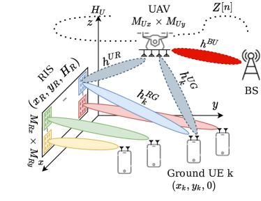
Figure 1: The problem scenario

To summarize, in this paper we explore the possibility of the combined usage of UAVs and RISs to reduce the energy consumption of the entire system, while providing a certain level of QoS to the UEs in the area. Figure 1 denotes the overall scenario in question. The UAV acts as a mobile BS relay that can establish Line-of-Sight (LoS) links with the UEs and the RIS, something that might not be always possible for the fixed BS.The UAV hence extends the area of coverage of the BS, while optimizing the energy consumption for in-flight movement and signal transmission due to the inclusion of the RIS. If the RIS position is optimal, which is another open research problem, the UEs can be served either directly by the UAV or with the help of the RIS or therefore combination of both, potentially reducing the energy consumption for in-flight movement of the UAVs. This can potentially extend the area of coverage (i.e., of the area of satisfactory QoS), also in situations where a BS could not be relied upon for service, such as emergency or disaster scenarios [4].

The contributions of this work are:

• Defining a scenario and solving the associated optimization problem with respect to UAV trajectory, RIS phase shift and BS-UAV link capacity limitation due to the UAV motion to provide at least a minimum guaranteed QoS to the UEs.

• Minimization of the transmission power of UAV and BS by jointly optimizing the UAV trajectory and the RIS phase shift.

The paper is structured as follows: Sec. I provides introduction and motivation for the usage of UAVs and RIS in cellular networks. Sec. II explains the optimization scenario and provides a brief formulation of the optimization problem whose solution is outlined in Sec. III. Sec. IV reports the simulation results for the obtained solution and the related discussion. Sec. V provides the conclusion and future research directions.

Notations

Italic lowercase letter a is a scalar. $\|a\|$ is a norm-two of a vector. $(\cdot)^{T}$ and $(\cdot)^{H}$ are transpose and Hermitian (conjugate transport), respectively. $\otimes$ is a Kronecker product. $\mathbb{C}$ is the complex numbers set.

II Scenario Definition and Problem Formulation

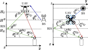
Figure 2: The vertical (left) and horizontal (right) AoDs/AoAs between the UAV, RIS, and $k^{th}$ UE in the downlink communication system respectively.

Consider a network environment with $K$ UEs randomly spread in the area, a RIS in fixed and known position. We make the following assumptions:

• User association and additional control information needed for data transfer are exchanged between BS and UEs by means of a dedicated long range control channel.

• UEs are aware of their own position (e.g., calculated through triangulation with respect to the BSs and UAVs in the area).

• The UEs periodically communicate their position to the BS that analyses this information to devise mobility patterns and traffic requirements in the environment.

• BSs, UAVs and UEs are equipped with Uniform Planar Square Array (UPA) antennas so as to perform concurrent beamforming in different directions.

• An extra large scale massive MIMO (XL-MIMO) RIS deployment is considered in which every UE is served by a specific region of the surface. This holds when the RIS dimensions is large and the UEs are sufficiently spaced apart to have partial observability of the surface [17].

II-1 Channel Models

As visible from Figure 1, there are four channels in the scenario: BS to UAV, UAV to UE, UAV to RIS and RIS to UE. The channel gains are denoted as $\mathrm{h}^{BU}$, $\mathrm{h}_{k}^{UG}$, $\mathrm{h}^{UR}$ and $\mathrm{h}_{k}^{RG}$ respectively and their derivation is detailed in Appendix I. The Signal-to-Noise Ratio (SNR) at the UAV with respect to the associated BS is given by,

$$\mathrm{\gamma}[n]=\frac{P^{T}_{BS}{|\mathrm{h}^{\mathrm{BU}}[n]|}^{2}}{\sigma^{2}_{n}},$$ (1)

where $\mathrm{P}_{\lx@glossaries@gls@link{acronym}{bs}{\leavevmode BS}}^{T}$ is the transmit power of the BS and $\sigma_{n}^{2}$ is the white noise power. Communication using (1) and assuming a Gaussian channel with an SNR of $\gamma[n]$, the maximum achievable rate of the BS to UAV channel is given by the Shannon bound:

$$C[n] =\log_{2}(1+\gamma[n])\qquad[\mathrm{bits/s/Hz}].$$ (2)

Note that, to use the above formula, we must assume that both UAV and BS know the channel between them and can determine the rate based on the available SNR. Also, we assume that the UEs are sufficiently spread apart to avoid mutual interference when communicating with the UAV. The SNR at the $k^{th}$ UE for the UAV to UE LoS link is given by,

$$\mathrm{\gamma}_{k,1} =\frac{P^{T}_{k}{|\mathrm{h}^{\mathrm{UG}}_{k}[n]|}^{2}}{\sigma^{2}_{n}},$$ (3)

where $P^{T}_{k}$ is the transmit power of the UAV towards the $k^{th}$ UE. Finally, the SNR at the $k^{th}$ UE from the UAV through the RIS (forming a cascade channel) is given by,

$$\mathrm{\gamma}_{k,2} =\frac{P^{T}_{k}{|\mathrm{H}^{\mathrm{URG}}_{k}[n]|}^{2}}{\sigma^{2}_{n}},$$ (4)

where $\mathrm{H}^{\mathrm{URG}}_{k}[n]$ is the overall channel gain of the cascade channel from UAV to RIS to UE. To be noted that, to limit the number of optimization parameters, we assume that the UAV transmits with the same power $P^{T}_{k}$ on both the direct and indirect (through RIS) channel to the $k^{th}$ UE. Detailed explanation to determine $\mathrm{H}^{\mathrm{URG}}_{k}[n]$ is given in Appendix I. Assuming, multiple RF chains in the UAV enough to serve multiple UEs in the environment directly and using the RIS, the total maximum achievable rate in [$bits/s/Hz$] at the $k^{th}$ UE from the UAV can be computed as

$$R_{k}=\sum_{i=1}^{2}R_{k,i} =\log_{2}((1+\gamma_{k,1})(1+\gamma_{k,2})),$$

$$\mathrm{where}$$

$$R_{k,1} =\log_{2}(1+\gamma_{k,1}),$$

$$R_{k,2} =\log_{2}(1+\gamma_{k,2}).$$

Hence, the scenario can be considered as an alternative to a Spatial Multiplexing scheme where the RIS redirects the signal from the UAV to the $k^{th}$ UE thereby potentially achieving the rate shown in (II-1).

II-2 Energy Consumption for UAV

TABLE I: Notation for Energy Consumption Model[5]

Symbol	Meaning	Simulation Values
$\Omega$	Blade Angular Velocity	$300~{}rad/s$
$r$	Rotor radius	$0.4~{}m$
$\rho$	Air Density	$1.225~{}kg/m^{3}$
$s$	Rotor Solidity	$0.05~{}m^{3}$
$A_{r}$	Rotor Disc Area	$0.503~{}m^{3}$
$v_{0}$	Induced velocity for rotor in forwarding flight	$4.03~{}m^{3}$
$d_{0}$	Fuselage drag ratio	$0.3$
$P_{0}$	Blade profile power in hovering status	$79.86~{}W$
$P_{i}$	Induced power in hovering status	$88.63~{}W$

The power consumption for UAV is critical due to its limited battery capacity. In the paper, we use the distance-based energy consumption model from [18] given by,

$$\mathrm{P}^{UAV}[n]=\underbrace{P_{o}\left(1+\frac{3\|\mathbf{v}[n]\|^{2}}{\Omega^{2}r^{2}}\right)}_{\mathrm{Bladeprofile}}+\underbrace{\frac{P_{i}v_{0}}{\|\mathbf{v}[n]\|}}_{\mathrm{Induced}}+\underbrace{\frac{1}{2}d_{0}\rho sA_{\mathrm{r}}\|\mathbf{v}[n]\|^{3}}_{\mathrm{Parasite}},$$ (6)

where $\mathbf{v}[n]$ is the velocity vector, and the other terms of the equation are explained in Tab. I. We only considered the energy consumption for the in-flight movement of the UAV for now and keep the impact of take off and landing on energy consumption for further research.

II-3 Optimization Problem

Considering the assumptions, the objective is to find an energy efficient UAV path and corresponding RIS phase shift in order to minimize the overall transmission power consumption of UAV and BS under minimum QoS constraints and maximum UAV energy budget which is defined as,

$$\min_{\mathbf{P},\mathbf{Z},\mathbf{V},\mathbf{\Phi}}~{} \sum_{n=1}^{N}\sum_{k=1}^{K}\mathrm{P}^{T}_{k}[n]+\sum_{n=1}^{N}\mathrm{P}^{T}_{BS}[n]$$ (7)

$$s.t.$$

$$C1:~{} R_{k}[n]\geq R_{min},\forall~{}k,n;$$

$$C2:~{} C[n]\geq\sum_{k=1}^{K}R_{k}[n],~{}\forall~{}n;$$

$$C3:~{} 0\leq\mathbf{\Phi}[n]\leq 2\pi;$$

$$C4:~{} \sum_{n=1}^{N}\mathrm{P}^{\lx@glossaries@gls@link{acronym}{uav}{\leavevmode UAV}}[n]\leq\mathrm{E}^{\lx@glossaries@gls@link{acronym}{uav}{\leavevmode UAV}}_{max};$$

$$C5:~{} \mathbf{Z}[n+1]=\mathbf{Z}[n]+\mathbf{v}[n]\tau,~{}n=1,\dots,N-1;$$

$$C6:~{} \|\mathbf{v}[n]\|\leq V_{max},~{}\forall n;$$

$$C7:~{} \|\mathbf{v}[n+1]-\mathbf{v}[n]\|\leq V_{acc}\tau,~{}n=1,\dots,N-1;$$

$$C8:~{} \|\mathbf{v}[n]\|\geq 0~{}\forall n;$$

$$C9:~{} \mathbf{Z}[1]=\mathbf{Z}_{0};$$

$$C10:~{} \mathbf{Z}[N]=\mathbf{Z}_{F}.$$

Optimization Variables

The terms of this optimization problem are explained below:

• $\mathbf{P}$: UAV ($\mathrm{P}^{T}_{k}$) and BS ($\mathrm{P}^{T}_{BS}$) transmission power.

• $\mathbf{Z}$: UAV trajectory, represented as the sequence of geographical coordinates of the UAV at each timestep.

• $\mathbf{V}$: UAV velocity over the trajectory.

• $\mathbf{\Phi}$: RIS phase configurations.

Objective Function

The objective is to minimize the overall energy consumption of UAV and BS for transmission during the $N$ timesteps taken by the UAV to cover its trajectory.

Constraints

C1–Guaranteed Rate Constraint

C1 is devised to provide a guaranteed service rate to each one of the $K$ UEs. We recall that $R_{k}$ is the sum rate achieved over the LoS and RIS link, which has to stay above the guaranteed rate $R_{min}$.

C2–Backhaul Capacity Constraint

C2 ensures that the backhaul link capacity is greater than or equal to the aggregate minimum guaranteed rate for all the UEs, i.e., that the UAV has enough bandwidth capacity towards the BS to provide at least the minimum guaranteed rate to all the UEs.

C3–Phase Shift Constraint

C3 limits the phase shift with respect to the incident signal from $0$ to $2\pi$. With the assumption of XL-MIMO surface for RIS, the phase shift can be considered almost continuous from $0$ to $2\pi$.

C4–UAV Energy Budget

C4 requires that the total energy consumption of the UAV over $N$ timesteps does not exceed the threshold $E^{UAV}_{max}$ that defines the maximum energy the UAV can spend before recharging and, implicitly, the maximum length of the UAV path.

C5–Timestep Position Constraint

C5 constraints the position $\mathrm{Z}[n]$ in successive timesteps, thereby limiting the movement of the UAV in one timestep.

C6–Maximum Velocity Constraint

C6 is devised to constraint the velocity $\mathbf{v}[n]$ of the UAV in one timestep to be lower than or equal to the maximum velocity $V_{max}$, thereby limiting the maximum distance the UAV can travel in one timestep.

C7–Timestep Velocity Constraint

C7 is devised to determine the velocity $\mathbf{v}[n]$ of the UAV in successive timesteps based on the maximum acceleration $V_{acc}$ of UAV in one timestep.

C8–Minimum Velocity Constraint

C8 constraints the velocity $\mathbf{v}[n]$ of the UAV, thereby limiting the minimum distance the UAV can travel over one timestep. Note that, if the UAV can hover at one place in one timestep, then the minimum velocity is zero.

C9/C10–Initial/Final Position Constraint

C9 and C10 fix the starting and ending points of the trajectory otherwise determined by the optimization problem.

We remark that, as shown in Figure 1 the UAV has two parallel links to each UE: one directional and the other with the RIS sector associated to the UE. The multipath approach offers a greater chance to satisfy the service requirement by jointly optimizing the UAV trajectory $\mathbf{Z}[n]$ and RIS phase configuration $\mathbf{\Phi}$, while minimizing the transmission power of the entire system. To facilitate the UEs to determine the multipath connections, the BS has to continuously communicate the beams to be used to the UE taking into account the mobility information of the UEs and the trajectory of the UAV. As mentioned before, the BS may communicate this information over long-range low-rate technologies such as LoRa [19].

III Analytical Solution

The optimization problem discussed in the previous section is clearly non-convex and, hence, quite difficult to solve in itself. But we can determine a feasible solution by considering the initial transmission powers for the UAV and BS so as to jointly optimize the UAV trajectory and RIS phase and, then, minimize the transmission powers for the given trajectory and phase configuration within the constraints in (7). This method is explained in detail in the following subsections.

III-A Joint UAV Trajectory and RIS phase optimization

Joint UAV Trajectory and RIS phase optimization can be facilitated considering a particular $\mathbf{P}$ over different links [20]. As shown in the Figure 2, the BS to UAV, UAV to UE, UAV to RIS and RIS to UE links are assumed to be deterministic LoS channels. For ease of notation, in the following we indicate the nodes involved in a link using the subscript $U$, $B$, $R$ and $G$ for UAV, BS, RIS and (ground) UE, respectively. The channel information is supposed to be available at the UAV and the UEs. Hence, to maximise the transmission efficiency, a Maximum Ratio Transmission (MRT) is applied, i.e., the transmission beamformer for any $k^{th}$ UE as well as for the UAV can be defined as $\mathrm{w^{BU}}=\frac{1}{\sqrt{M_{B}}}\mathrm{h^{BU}},\mathrm{w^{UG}_{k}}=\frac{1}{\sqrt{M_{U}}}\mathrm{h^{UG}}$ and $\mathrm{w^{UR}}=\frac{1}{\sqrt{M_{U}}}\mathrm{h^{UR}}$. The overall channel gains can hence be obtained as,

$$\mathrm{H^{BU}}[n] =(\mathrm{h^{BU}}[n])^{\mathrm{H}}[n]\mathrm{w^{BU}}[n]=\frac{\sqrt{M_{\mathrm{B}}}\alpha_{0}}{d^{\mathrm{BU}}[n]};$$ (8)

$$\mathrm{H^{UG}_{k}}[n] =(\mathrm{h^{UG}_{k}}[n])^{\mathrm{H}}[n]\mathrm{w^{UG}_{k}}[n]=\frac{\sqrt{M_{\mathrm{U}}}\alpha_{0}}{d_{k}^{\mathrm{UG}}[n]};\$$ (9)

$$\mathrm{H^{URG}_{k}}[n] =(\mathrm{h_{k}^{\mathrm{RG}}}[n])^{\mathrm{H}}\mathbf{\Phi}_{k}[n]\mathrm{H}^{\mathrm{UR}}[n]\mathrm{w^{UR}}[n]$$

$$=\sqrt{M_{\mathrm{U}}}(\mathrm{h_{k}^{\mathrm{RG}}}[n])^{\mathrm{H}}\mathbf{\Phi}_{k}[n]\mathrm{h^{\mathrm{RU}}}[n]$$

$$=\frac{\sqrt{M_{\mathrm{U}}}M_{\mathrm{R}}\alpha_{0}}{d_{k}^{\mathrm{RG}}d^{\mathrm{UR}}[n]}.$$ (10)

To determine the $\mathrm{H^{URG}_{k}}[n]$ coefficients correctly, the optimal phase control policy for the phase shift in every timestep (which maximizes the reflection-mode channel gain by aligning the phase of the RIS to match those of the channel) is given by,

$$\mathbf{\Phi}_{m_{\mathrm{R}x},m_{\mathrm{R}y},k}=\frac{2\pi\Delta_{\mathrm{R}}}{\lambda_{\mathrm{c}}}[(m_{\mathrm{R}x}-1)(\sin\theta^{\mathrm{RU}}\cos\xi^{\mathrm{RU}}$$

$$+\sin\theta_{k}^{\mathrm{RG}}\cos\xi_{k}^{\mathrm{RG}})+(m_{\mathrm{R}y}-1)(\sin\theta^{\mathrm{RU}}\sin\xi^{\mathrm{RU}}$$

$$+\sin\theta_{k}^{\mathrm{RG}}\sin\xi_{k}^{\mathrm{RG}})],$$ (11)

where $\theta^{\mathrm{RU}}$ and $\xi^{\mathrm{RU}}$ are the Angle of Arrivals (AoAs) and $\theta^{\mathrm{RG}}$ and $\xi^{\mathrm{RG}}$ are the Angle of Departures (AoDs) as defined in Figure 2. The assumption for RIS phase configuration is that there is a wired direct link to the RIS controller and that, delay and imperfect phase configuration are negligible.
Note that, the problem is still non-convex due to C1 and C2 w.r.t. $\mathbf{Z}$. In order to overcome this issue, we add three slack variables $\lambda_{k,i}[n]$, $\mu[n]$ and $\pi[n]$. In this way, we keep the constraints C1-9, and the problem can be reformulated as follows,

$$\min_{\mathbf{Z},\mathbf{V},\mathbf{\Lambda},\mathbf{M},\mathbf{\Pi}}~{} \sum_{k=1}^{K}\sum_{n=1}^{N}\mathrm{P}^{T}_{k}[n]+\sum_{n=1}^{N}\mathrm{P}^{T}_{BS}[n]$$ (12)

$$s.t.$$

$$C1-~{} C10;$$

$$C11:~{} \|\mathbf{Z}_{k}^{\lx@glossaries@gls@link{acronym}{ue}{\leavevmode UE}}-\mathbf{Z}[n]\|^{2}\leq\lambda_{k,1}[n],k\in\{1,...,K\};$$

$$C12:~{} \|\hat{\mathbf{Z}}_{k}^{\lx@glossaries@gls@link{acronym}{ris}{\leavevmode RIS}}-\mathbf{Z}[n]\|^{2}\leq\lambda_{k,2}[n],k\in\{1,...,K\};$$

$$C13:~{} \|\mathbf{Z}^{\lx@glossaries@gls@link{acronym}{bs}{\leavevmode BS}}-\mathbf{Z}[n]\|^{2}\leq\mu[n];$$

$$C14:~{} \|\mathbf{v}[n]\|^{2}\geq\pi^{2}[n];$$

$$C15:~{} \pi[n]\geq 0;$$

where $\mathbf{\Lambda}=\{\lambda_{k,i}[n],\forall~{}n,k,i\}$, $\mathbf{M}=\{\mu[n],\forall~{}n,l\}$ and $\mathbf{\Pi}=\{\pi[n],\forall~{}n\}$. Similarly to what proposed in [5], we overcome the non-convex constraints C1 and C2 via Successive Convex Approximation (SCA) in an iterative way. We can compute a lower bound of the instant achievable rate for each user by modifying $\lambda_{k,i}[n]$, $\mu[n]$ and $\pi[n]$ and calculating the first-order Taylor expansion which is a global under-estimator of the rate convex function [21]. Hence, omitting the argument $[n]$ for notation clarity, we redefine the SNR expression as,

$$\gamma_{k,i} =\frac{\hat{\gamma}_{k,i}}{\lambda_{k,i}},i=1,2;$$ (13)

$$\gamma =\frac{\hat{\gamma}}{\mu};$$ (14)

where

$$\hat{\gamma} =\frac{\mathrm{P}^{T}_{BS}\mathrm{M_{B}}\alpha^{2}_{0}}{\sigma^{2}_{n}};$$ (15)

$$\hat{\gamma}_{k,1} =\frac{\mathrm{P}^{T}_{k}\mathrm{M_{U}}\alpha^{2}_{0}}{\sigma^{2}_{n}};$$ (16)

$$\hat{\gamma}_{k,2} =\frac{\mathrm{P}^{T}_{k}\mathrm{M_{U}}\mathrm{M^{2}_{R}}\alpha^{2}_{0}}{(d^{\mathrm{RG}}_{k})^{2}\sigma^{2}_{n}}.$$ (17)

Hence, the maximum achievable instant rate per link $i$ for $k^{th}$ UE from the UAV is given by,

$$\hat{R}_{k,i}[n] =\log_{2}(1+\gamma_{k,i}[n]),$$ (18)

Similarly, the capacity at the UAV from BS is given by,

$$\hat{C}[n] =\log_{2}(1+\gamma[n]).$$ (19)

Applying the first-order Taylor expansions in the $j$-th iteration for a particular value of $\lambda_{k,i}^{j}[n]$, $\mu^{j}[n]$ and $\mathbf{v}^{j}[n]$ in (18) and (19), the lower bound for the rates is given by,

$$\hat{R}_{k,i}[n]\geq$$

$$(\hat{R}_{k,i}[n])^{j}= ~{}\log_{2}\left(1+\frac{\gamma_{k,i}[n]}{\lambda_{k,i}^{j}[n]}\right)$$

$$-\frac{\gamma_{k,i}[n](\lambda_{k,i}[n]-\lambda_{k,i}^{j}[n])}{\lambda_{k,i}^{j}[n](\lambda_{k,i}^{j}[n]+\gamma_{k,i}[n])\ln 2},$$ (20)

$$\hat{C}[n]\geq$$

$$(\hat{C}[n])^{j}= ~{}\log_{2}\left(1+\frac{\gamma[n]}{\mu^{j}[n]}\right)$$

$$- \frac{\gamma[n](\mu[n]-\mu^{j}[n])}{\mu^{j}[n](\mu^{j}[n]+\gamma[n])\ln 2},$$ (21)

$$\|\mathbf{v}[n]\|^{2}\geq ~{}\|\mathbf{v}^{j}[n]\|^{2}+2[\mathbf{v}^{j}[n]]^{\mathrm{T}}(\mathbf{v}[n]-\mathbf{v}^{j}[n]).$$ (22)

where $(\hat{R}_{k,i}[n])^{j}$ and $(\hat{C}[n])^{j}$ are the lower bound achievable rates for the $k^{th}$ UE and UAV respectively, in the $j^{th}$ iteration of SCA.
Additionally, the total transmission energy consumed over the whole trajectory can be represented as,

$$\mathrm{P}^{Total}= \sum_{k=1}^{K}\sum_{n=1}^{N}\mathrm{P}^{T}_{k}[n]+\sum_{n=1}^{N}\mathrm{P}^{T}_{BS}[n],$$ (23)

Also, the in-flight power consumption for UAV can be written as,

$$\mathrm{P}^{UAV}[n] =P_{o}\left(1+\frac{3\|\mathbf{v}[n]\|^{2}}{\Omega^{2}r^{2}}\right)+\frac{P_{i}v_{0}}{\pi[n]}+\frac{1}{2}d_{0}\rho_{s}A_{\mathrm{r}}\|\mathbf{v}[n]\|^{3}.$$ (24)

Applying the lower bounds in (20), (21) and (22) in (12) we obtain a convex problem defined as,

$$\min_{\mathbf{Z},\mathbf{V},\mathbf{\Lambda},\mathbf{M},\mathbf{\Pi}} ~{}\mathrm{P}^{Total}$$ (25)

$$s.t.$$

$$\hat{C}1: ~{}\sum_{i=1}^{2}(\hat{R}_{k,i}[n])^{j}\geq R_{min},\forall~{}k;$$

$$\hat{C}2: ~{}(\hat{C}[n])^{j}\geq\sum_{k=1}^{K}\sum_{i=1}^{2}(\hat{R}_{k,i})^{j}[n];$$

$$\hat{C}14: ~{}\|\mathbf{v}^{j}[n]\|^{2}+2[\mathbf{v}^{j}[n]]^{\mathrm{T}}(\mathbf{v}[n]-\mathbf{v}^{j}[n])\geq\pi^{2}[n];$$

$$C3 -C15,$$

which solving it provides an upper bound of the problem in (12). We iteratively update the feasible solution $\mathbf{Z}^{j}[n]$, $\lambda_{k,i}^{j}[n]$, $\mu^{j}[n],\mathbf{v}^{j}[n]$ and $\pi^{j}[n]$ by solving the convex problem in (25) using the CVX standard optimization solver [22] in the $j$-th iteration.

III-B Transmission Power Control

For a determined UAV trajectory and RIS phase, the UAV and BS transmission power can be minimized. To define the transmission power minimization with a predefined trajectory $\mathbf{Z}$, the optimization problem in (7) can be rewritten with constraints $C3-C10$ already satisfied for the pre-defined trajectory $\mathbf{Z}$. So the optimization problem can be written as,

$$\min_{\mathbf{P}}~{} \mathrm{P}^{Total}$$ (26)

$$s.t.$$

$$C1:~{} \sum_{i=1}^{2}R_{k,i}[n]\geq R_{min},\forall~{}k,n;$$

$$C2:~{} C[n]\geq\sum_{k=1}^{K}\sum_{i=1}^{2}R_{k,i}[n],~{}\forall~{}n.$$

The constraints $C1$ and $C2$ are concave with respect to the $\mathbf{P}$. Hence it can be easily solved by employing SCA using the Taylor’s expansions of (18) and (19), which are global over-estimators of the concave functions. To do so, the SNR expressions are rewritten as,

$$\gamma_{k,i}[n] =\mathrm{P}^{T}_{k,i}[n]\kappa_{k,i}[n],\forall~{}i\in\{1,2\},~{}k;$$ (27)

$$\gamma[n] =\mathrm{P}^{T}_{BS}[n]\kappa[n];$$ (28)

where,

$$\kappa_{k,1}[n] =\bigg{\{}\frac{\sqrt{M_{\mathrm{U}}}\alpha_{0}}{d_{k}^{\mathrm{UG}}[n]\sigma}\bigg{\}}^{2},$$ (29)

$$\kappa_{k,2}[n] =\bigg{\{}\frac{\sqrt{M_{\mathrm{U}}}M_{\mathrm{R}}\alpha_{0}}{d_{k}^{\mathrm{RG}}d^{\mathrm{UR}}[n]\sigma}\bigg{\}}^{2},$$ (30)

$$\kappa[n] =\bigg{\{}\frac{\sqrt{M_{\mathrm{B}}}\alpha_{0}}{d^{\mathrm{BU}}[n]\sigma}\bigg{\}}^{2}.$$ (31)

The first-order Taylor expansion for (18) and (19) yields,

$$\hat{R}_{k,1}[n]\leq$$

$$(\hat{R}_{k,2}[n])^{j}= ~{}\log_{2}\left(1+(\mathrm{P}^{T}_{k,1})^{j}{|\kappa_{k,1}[n]|}^{2}\right)$$

$$+\frac{{|\kappa_{k,1}[n]|}^{2}(\mathrm{P}^{T}_{k,1}-(\mathrm{P}^{T}_{k,1})^{j})}{(1+(\mathrm{P}^{T}_{k,1})^{j}{|\kappa_{k,1}[n]|}^{2})\ln(2)},$$ (32)

$$\hat{R}_{k,2}[n]\leq$$

$$(\hat{R}_{k,2}[n])^{j}= ~{}\log_{2}\left(1+(\mathrm{P}^{T}_{k,2})^{j}{|\kappa_{k,2}[n]|}^{2}\right)$$

$$+\frac{{|\kappa_{k,2}[n]|}^{2}(\mathrm{P}^{T}_{k,2}-(\mathrm{P}^{T}_{k,2})^{j})}{(1+(\mathrm{P}^{T}_{k,2})^{j}{|\kappa_{k,2}[n]|}^{2})\ln(2)},$$ (33)

$$\hat{C}[n]\leq$$

$$(\hat{C}[n])^{j}= ~{}\log_{2}\left(1+(\mathrm{P}^{T}_{BS})^{j}{|\kappa[n]|}^{2}\right)$$

$$+\frac{{|\kappa_{l}[n]|}^{2}(\mathrm{P}^{T}_{BS}-(\mathrm{P}^{T}_{BS})^{j})}{(1+(\mathrm{P}^{T}_{BS})^{j}{|\kappa[n]|}^{2})\ln(2)},$$ (34)

Hence, the optimization problem (26) can be rewritten as,

$$\min_{\mathbf{P}}~{} \mathrm{P}^{Total}$$ (35)

$$s.t.$$

$$C1:~{} \sum_{i=1}^{2}(\hat{R}_{k,i}[n])^{j}[n]\geq R_{min},\forall~{}k,n;$$

$$C2:~{} (\hat{C}[n])^{j}[n]\geq\sum_{k=1}^{K}\sum_{i=1}^{2}(\hat{R}_{k,i})^{j}[n],~{}\forall~{}n.$$

Similar to the UAV trajectory and RIS phase optimization problem, this optimization can be solved using the CVX standard optimization solver. Algorithm 1 provides the pseudocode to solve the optimization problem. Note that, we are aiming to minimize the transmission energy consumption of the UAV and BS by iteratively choosing a UAV route aided by the phase shifting involved in the RIS, which satisfies a target minimum rate for all the users, taking into account the rate aggregation of all the users is achievable, fulfilling the backhaul link capacity limitation, something not addressed in the literature to the best of the authors’ knowledge.

Result: UAV Trajectory $\mathbf{Z}$, UAV Velocity $\mathbf{V}$, $\mathrm{P}^{Total}$

Initialize trajectory $\mathbf{Z}$, $\mathbf{V}$, maximum number of iteration $J_{max}$, initial iteration index $j=0$, Particular UAV and BS transmission power $\mathbf{P}$ , Initial trajectory $\mathbf{Z}$, Initial velocity $\mathbf{V}$ and Convergence tolerance $\epsilon$;

while $j~{}\leq~{}J_{max}$ or $\dfrac{\mathrm{P}_{Total}^{j}-\mathrm{P}_{Total}^{j-1}}{\mathrm{P}_{Total}^{j}}\leq\epsilon$  do

       Set $j=j+1$ and $\{\mathbf{P}^{j},\mathbf{V}^{j},\mathbf{\Lambda}^{j},\mathbf{M}^{j},\mathbf{\Pi}^{j}\}=\{\mathbf{P},\mathbf{V},\mathbf{\Lambda},\mathbf{M},\mathbf{\Pi}\}$;

       Solving optimization problem (25) to obtain $\mathbf{Z},\mathbf{V},\mathbf{\Lambda},\mathbf{M}$ and $\mathbf{\Pi}$ for a Particular $\mathbf{P}$;

       Solving optimization problem (35) to obtain $\mathbf{P}$ and $\mathrm{P}_{Total}$ for a Particular $\mathbf{Z},\mathbf{V},\mathbf{\Lambda},\mathbf{M},\mathbf{\Pi}$

       Update $\mathrm{P}_{Total}^{j}=\mathrm{P}_{Total}$;

      

end while

Algorithm 1 Joint Trajectory, RIS Phase Configuration and Transmission Power Control algorithm

IV Results and Discussion

The solution discussed in the previous section is implemented in MATLAB simulation environment. The base simulation parameters are defined by Tab. II.

IV-A Simulation Environment

TABLE II: Simulation Parameters

Parameter	Value
Area	500m $\times$ 500m
Number of Users (K)	3
Position of Users	[20, 450; 250, 0; 500, 200]
Position of Base Station	[0, 0]
Number of UAVs	1
Initial/Final Position of UAV ($\mathrm{Z}_{0}/\mathrm{Z}_{F}$)	[0, 0; 500, 500]
Maximum Velocity	20 m/s
Maximum Acceleration	4 m/s2
Height of the [UAV, BS, RIS]	[20,15,10] m
Path Loss ($\alpha_{0}$)	61 dBm
Noise Power Spectral Density ($\sigma^{2}$)	-174 dBm

At this stage of the work, we only considered scenarios with static UEs. The analysis of the system performance in presence of mobile UEs is left to future work. The simulation results are categorised under five different evaluation scenarios:

• UAV LoS transmission power v/s UAV RIS transmission power: The evaluation scenario shows the transmission power necessary to be used using the LoS link and the RIS link.

• Impact of RIS Position on UAV Trajectory: The scenario studies the impact of the RIS position on the UAV trajectory.

• Impact of RIS Position on UAV LoS Transmission Power: The scenario analyzes the impact of the RIS position on the LoS transmission power consumption when vary the minimum rate requirements.

• Impact of RIS Position on UAV Trajectory Power Consumption: The scenario summarises the UAV trajectory power consumption for different UE minimum rate requirements.

• Impact of UAV Energy Budget on UAV Trajectory: The scenarios shows the impact of the total energy budget $E^{UAV}_{max}$ for the UAV trajectory.

The simulation environment (with parameters denoted in Tab. II) is shown in the Figure 3. As visible from the figure, over the SCA iterations, the UAV trajectory and transmission power is optimized using Algorithm 1 until it converges, i.e., UAV trajectory and transmission power are no longer improved.

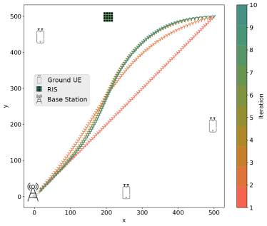
Figure 3: Optimization of the UAV trajectory and transmission power over SCA iterations. The marked lines represent the UAV trajectories obtained during the execution of the iterative algorithm. The straight line is the initial solution, while the darkest one is the final solution.

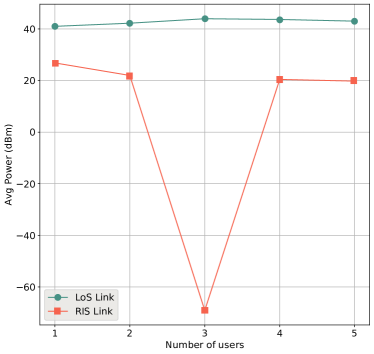
Figure 4: Average Power Consumption over UAV LoS and RIS links towards the UEs, for increasing number of static UEs and with a constant minimum rate requirement $R_{min}$.

IV-B UAV LoS Transmission Power v/s UAV RIS Transmission Power

Different configurations in terms of static number of UEs in the network have been simulated. Figure 4 shows the average transmission power per timestep along the optimized trajectory for both the LoS and the RIS links for $K$ UEs. The first observation is the transmission power over RIS link is significantly lower than that over LoS. This shows the fundamental role of the $M_{R}^{2}$ factor in (17) to help provide good SNR conditions. The results show that, in general, the average transmission power over the LoS link is slightly increasing for $K\leq 3$ and then slightly decreasing for $K>3$. Also, there are significant changes in the RIS link. It is noticed that the transmission power for LoS link (bullet-marked) generally increases for $K\leq 3$ UEs, i.e., LoS link is preferred, while, when $K>3$, the RIS link is preferred reducing the LoS contribution to fulfill the constraints while increasing in the RIS link transmission power. Additionally, the sudden drop in average power consumption for RIS link for three UEs is because the RIS is far away from the UEs as visible from Figure 3. Hence, the system is very sensitive to the RIS position. The variations in the RIS link also shows the importance of its usage, as it adapts to the environment providing less or more power in order to fulfill the constraints. This shows the potential impact of RIS in terms of total power minimization and scalability of the system. Looking at the total transmission power used along the optimized trajectory, that is, the summation of the power from the BS and the transmission power for the UAV, Figure 5 shows now that the power increases with the number of users in the network for different values of $R_{min}$. To be noted that the curve bends when the number of users increases, since their distance to the BS, UAV and RIS reduces. Also, the total power increases with the minimum rate requirement. Another significant observation is the change in average power consumption per set of users for different rates. The change in principle should be exponential, i.e., linear increase in rate should require exponential increase in power. But, to follow this criteria, the distance has to be constant, i.e., the trajectory of the UAV has to be constant for all the different rates. But, as visible in Figure 6, which shows the optimal trajectories for different values of $R_{min}$, the optimal trajectory for $R_{min}=0.057$ is able to deviate more from the straight line trajectory as it can still satisfy the low required minimum rate for the UEs. On the contrary, the optimal trajectory for $R_{min}=0.757$ is able to deviate less from the straight line trajectory than that for $R_{min}=0.057$ as the required minimum rate is higher. Note that, we only show optimal trajectories for $R_{min}=\{0.057,0.257,0.557,0.757\}$ to be able to visually distinguish between the optimal trajectories for the different values of $R_{min}$. The optimal trajectories for the remaining values of $R_{min}$ are between the optimal trajectory for $R_{min}=0.057$ and $R_{min}=0.757$. This trend for optimal trajectories is also true for the scenarios involving one, two, four and five UEs. Hence, the average power consumption for UEs, as shown in Figure 5, does not follow an exponential criteria due to change in optimal trajectory for different values of $R_{min}$. Additionally, the system fails to find feasible solutions above five UEs, i.e., one UAV cannot serve more than five UEs simultaneously in a single flight in the considered scenario. The current configuration based on CVX, makes difficult to go beyond $R_{min}=0.757$. Then, the usage of reinforcement learning can be explored to improve scalability, which has been left for future work.

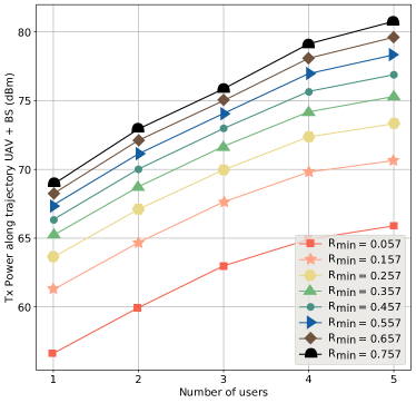
Figure 5: Total Transmission Power (UAV and BS) when increasing the number $K$ of static UEs for different values of $R_{min}$.

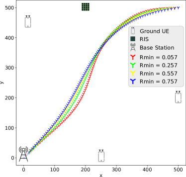
Figure 6: Different Optimal Trajectories for the UAV for three UEs and for different values of $R_{min}$.

IV-C Impact of RIS Position on UAV Trajectory

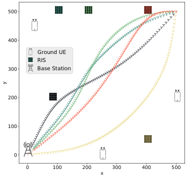
Figure 7: Impact of RIS position on UAV Trajectory for a fixed UE and BS positions

We analyze the impact of the different positions of RIS on the optimal UAV trajectories as shown in Figure 7. The first discernible observation is that the UAV attempts to go as close as possible to the RIS. This is because the transmission power necessary to satisfy the rate requirement of the UEs is considerably lower when using the RIS compared to directly transmitting to the UEs. This, however, is compensated by the higher path loss that is encountered by the signal i.e. the total distance the signal has to cover using the RIS is higher than that along the LoS channel. Due to this fact, the UAV cannot use the RIS to serve all the UEs at all timesteps. Hence some UEs has to be served directly. This creates a push-pull effect on the UAV that prevents the UAV to venture very close to one UE to avoid violating the QoE requirements of the other UEs. Hence, determining an optimal position for RIS is important while designing the network.

IV-D Impact of UAV Energy Budget on UAV Trajectory

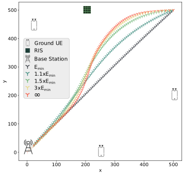
Figure 8: Impact of UAV Energy Budget on the UAV Trajectory

To study the impact of the energy budget on the UAV trajectory optimization, we determine the UAV trajectories for different energy budget values. The energy consumed by the UAV over the straight line path (i.e, shortest path) is the minimum in-flight energy consumption necessary for the UAV to reach its final destination and is hence set as a reference minimum $\mathrm{E_{min}}$. Hence, the energy budget for the UAV is defined as a multiple of $\mathrm{E_{min}}$. Figure 8 denotes the impact of UAV energy budget on the trajectory optimization. As visible from the figure, when increasing the budget, the UAV is able to deviate further away from the shortest path trajectory. But eventually, it cannot go much further as it would risk not serving the users on the opposite side (as discussed previously). Once the UAV energy is sufficient to draw the optimal trajectory across the area, any further increase of the UAV energy would likely allow the UAV to slow down its speed or hover on the optimal location for a longer time, thus improving the transmission energy efficiency of the system. The minimum amount of energy required to reach the optimal trajectory is hence important to dimension the UAV battery capacity.

IV-E Impact of RIS Position on UAV Transmission Power

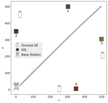
Figure 9: Different RIS positions configuration

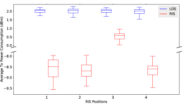
Figure 10: Average transmission power consumption of the UAV over the LoS and RIS link for different positions of the RIS as shown in Figure 9, for 50 different network service requirements.

As concluded in previous subsection, the UAV has a tendency to move towards the RIS. To determine the impact of the RIS position on the UAV transmission power consumption, we obtained the optimal trajectory for different network service requirements i.e. spectral efficiency or $R_{min}$ per UE randomly chosen between $0.01$ and $0.757$ bits/s/Hz. Figure 10 shows the boxplot for the average UAV power consumption over LoS and RIS links for different positions of the RIS, as denoted in Figure 9, obtained for 50 different sets of values of $R_{min}$ randomly chosen between $0.01$ and $0.757$ bits/s/Hz.

As visible from the figure, the RIS position is crucial with respect to not only the UEs but also the initial trajectory of the UAV. When in position 3, the RIS is closer to both the UEs and the UAV initial trajectory and hence the optimization problem uses the RIS link to serve the UEs. On the other hand, in position 2, the RIS is closer to the UE but is further away from the UAV initial trajectory and hence the RIS link is not much used by the UAV. In the other two positions, the RIS is extremely far away from the UEs and hence is also not much used.

So the optimal solution is able to use the RIS to serve the users when the RIS is closer to the UEs as well as the UAV initial trajectory. This also signifies that, the SCA is extremely sensitive to network configurations especially with respect to UAV initial trajectory and RIS and UEs positions. It also highlights a drawback in the usage of SCA. By using SCA to determine the optimal UAV trajectory, RIS phase and UAV transmission power, it is really dependent on the initial state (a.k.a trajectory) we decided to solve the optimization problem. Hence, the usage of data driven methods such as reinforcement learning techniques to jointly optimize the UAV trajectory, RIS phase and UAV transmission power can be extremely lucrative and pursued for further work, as it would provide a more generalized solution regardless of the specific network configuration.

V Conclusion

Beyond 5G and 6G Networks are expected to provide a certain service level while reducing the power consumption of the system. To this end, we discussed the usage of UAVs and RIS as a way to guarantee certain service requirements while trying to minimise the power consumption of the system.

In this work, we devised jointly, a method to roughly optimize UAV trajectory, RIS phase and UAV transmission power consumption to provide a certain guaranteed service rate to the UEs on the ground. We showed the usage of convex approximation techniques can provide a feasible solution.

Moving forward, the usage of reinforcement learning seems very attractive especially due to the sensitive nature of convex approximation schemes to different network configurations.

Appendix I

In Appendix I, the channel models incorporated in the optimization problem are presented.

V-1 BS to UAV ($h^{BU}$) Channel

We assume a LoS channel based on the UAV-UE channel model from [5]. From Figure 1, we devise $d^{\mathrm{BU}}[n]=\sqrt{\|\mathbf{Z}^{BS}-\mathbf{Z}[n]\|^{2}}$ as the Euclidean distances between UAV and BS where $\mathbf{Z}[n]=[x_{U}[n],y_{U}[n],H_{U}]$ and $\mathbf{Z}^{BS}=[x_{B},y_{B},H_{B}]$ are the coordinates of UAV and BS at a particular time instant $n$. So, the LoS channel from BS to UAV is designed as follows

$$\mathrm{h}^{\mathrm{BU}}[n] =\sqrt{\frac{\alpha_{0}}{(d^{\mathrm{BU}}[n])^{2}}}[1,e^{-j\frac{2\pi\Delta_{\mathrm{B}x}}{\lambda_{\mathrm{c}}}\sin\theta^{\mathrm{BU}}\cos\xi^{\mathrm{BU}}},$$

$$\ldots,e^{-j\frac{2\pi\Delta_{\mathrm{B}x}}{\lambda_{\mathrm{c}}}(M_{\mathrm{B}x}-1)\sin\theta^{\mathrm{BU}}_{k}\cos\xi^{\mathrm{BU}}}]^{\mathrm{H}}$$

$$\otimes[1,e^{-j\frac{2\pi\Delta_{\mathrm{B}y}}{\lambda_{\mathrm{c}}}\sin\theta^{\mathrm{BU}}\sin\xi^{\mathrm{BU}}},$$

$$\ldots,e^{-j\frac{2\pi\Delta_{\mathrm{B}y}}{\lambda_{\mathrm{c}}}(M_{\mathrm{B}y}-1)\sin\theta^{\mathrm{BU}}\sin\xi^{\mathrm{BU}}}]^{\mathrm{H}}\in\mathbb{C}^{M_{\mathrm{B}}\times 1}$$

where, $\mathbf{h}^{\mathrm{BU}}[n]$ is the channel vector based on the AoD. $\Delta_{\mathrm{Bx}}$ and $\Delta_{\mathrm{By}}$ are the separation between antenna elements in x-direction and y-direction for UE. Also, $M_{\mathrm{B}x}$ and $M_{\mathrm{B}y}$ is the number of antenna elements in x and y-direction for BS, $M_{\mathrm{B}}=M_{\mathrm{B}x}\times M_{\mathrm{B}y}$ is total number of antenna elements for BS and $\lambda_{\mathrm{c}}$ is the carrier wavelength. $\theta^{\mathrm{BU}}$ and $\xi^{\mathrm{BU}}$ are the AoD for the link from BS to the UAV. From Figure 2, it can be observed that $\sin\theta^{\mathrm{BU}}=\dfrac{\|H_{B}\|}{d^{\mathrm{BU}}}$, $\sin\xi^{\mathrm{BU}}=\dfrac{\|x_{B}-x_{U}[n]\|}{\|l_{B}-l_{U}[n]\|}$ and $\cos\xi^{\mathrm{BU}}=\dfrac{\|y_{B}-y_{U}[n]\|}{\|l_{B}-l_{U}[n]\|}$ where, $l_{B}=[x_{B},y_{B}]$ and $l_{U}[n]=[x_{U}[n],y_{U}[n]]$.

V-2 UAV to UE ($h^{UG}$) Channel

For the link between UAV and UE, which is LoS and between UAV and UE through RIS, we adopt the channel model from [5]. The UAV, RIS and UE, as previously mentioned, have a UPA antenna with $M_{\mathrm{U}},M_{\mathrm{R}}$ and $M_{\mathrm{G}}$ elements, respectively. Due to our XL-MIMO RIS assumption, the channel model we propose corresponds to each subsection/group of elements in the XL-MIMO RIS that we are using to serve different UEs, similar to the approach proposed in [23] to reflect sharp beams towards specific destinations. We assume that these groups have sufficient spatial separation thereby neglecting interference among them. From Figure 1, we devise $d^{\mathrm{UR}}=\sqrt{\|\mathbf{Z}^{RIS}-\mathbf{Z}[n]\|^{2}},~{}d_{k}^{\mathrm{UG}}=\sqrt{\|\mathbf{Z}_{k}^{UE}-\mathbf{Z}[n]\|^{2}},~{}\mathrm{and}~{}d_{k}^{\mathrm{RG}}=\sqrt{\|\mathbf{Z}^{RIS}-\mathbf{Z}_{k}^{UE}\|^{2}}$ as the Euclidean distances between UAV and RIS, UAV and $k^{th}$UE and RIS and $k^{th}$ UE respectively, where $\mathbf{Z}^{RIS}=[x_{R},y_{R},H_{R}]$ and $\mathbf{Z}_{k}^{UE}=[x_{G,k},y_{G,k},0]$ are the coordinates of RIS and $k^{th}$ UE. So, the LoS channel from UAV to UE is designed as follows,

$$\mathrm{h}^{\mathrm{UG}}_{k}[n] =\sqrt{\frac{\alpha_{0}}{(d^{\mathrm{UG}}_{k}[n])^{2}}}[1,e^{-j\frac{2\pi\Delta_{\mathrm{U}x}}{\lambda_{\mathrm{c}}}\sin\theta^{\mathrm{UG}}_{k}\cos\xi^{\mathrm{UG}}_{k}},$$

$$\ldots,e^{-j\frac{2\pi\Delta_{\mathrm{U}x}}{\lambda_{\mathrm{c}}}(M_{\mathrm{U}x}-1)\sin\theta^{\mathrm{UG}}_{k}\cos\xi^{\mathrm{UG}}_{k}}]^{\mathrm{H}}$$

$$\otimes[1,e^{-j\frac{2\pi\Delta_{\mathrm{U}y}}{\lambda_{\mathrm{c}}}\sin\theta^{\mathrm{UG}}_{k}\sin\xi^{\mathrm{UG}}_{k}},$$

$$\ldots,e^{-j\frac{2\pi\Delta_{\mathrm{U}y}}{\lambda_{\mathrm{c}}}(M_{\mathrm{U}y}-1)\sin\theta^{\mathrm{UG}}_{k}\sin\xi^{\mathrm{UG}}_{k}}]^{\mathrm{H}}\in\mathbb{C}^{M_{\mathrm{U}}\times 1}$$

where, $\mathrm{h}_{k}^{\mathrm{UG}}[n]$ is the channel vector based on the AoD and $\lambda_{c}$ is the carrier wavelength. $\theta^{\mathrm{UG}}_{k}$ and $\xi^{\mathrm{UG}}_{k}$ are the AoD for the link from UAV to $k^{th}$ UE. From Figure 2, it can be observed that $\sin\theta^{\mathrm{UG}}_{k}=\dfrac{\|H_{U}\|}{d^{\mathrm{UG}}_{k}}$, $\sin\xi^{\mathrm{UG}}_{k}=\dfrac{\|x_{G,k}-x_{U}[n]\|}{\|l_{G,k}-l_{U}[n]\|}$ and $\cos\xi^{\mathrm{UG}}_{k}=\dfrac{\|y_{G,k}-y_{U}[n]\|}{\|l_{G,k}-l_{U}[n]\|}$ where, $l_{G,k}=[x_{G,k},y_{G,k}]$ and $l_{U}[n]=[x_{U}[n],y_{U}[n]]$.

V-3 UAV to RIS to UE ($h^{URG}$) Channel

Similarly, the channel from UAV to RIS is defined as follows

$$\mathrm{H}^{\mathrm{UR}}[n] =\mathrm{h}^{\mathrm{RU}}[n]\otimes(\mathrm{h}^{\mathrm{UR}}[n])^{\mathrm{H}}$$

$$=\sqrt{\frac{\alpha_{0}}{(d^{\mathrm{UR}}[n])^{2}}}[1,e^{-j\frac{2\pi\Delta_{\mathrm{R}x}}{\lambda_{\mathrm{c}}}\sin\theta^{\mathrm{RU}}\cos\xi^{\mathrm{RU}}},$$

$$\ldots,e^{-j\frac{2\pi\Delta_{\mathrm{R}x}}{\lambda_{\mathrm{c}}}(M_{\mathrm{R}x}-1)\sin\theta^{\mathrm{RU}}\cos\xi^{\mathrm{RU}}}]^{\mathrm{H}}$$

$$\otimes[1,e^{-j\frac{2\pi\Delta_{\mathrm{R}y}}{\lambda_{\mathrm{c}}}\sin\theta^{\mathrm{RU}}\sin\xi^{\mathrm{RU}}},$$

$$\ldots,e^{-j\frac{2\pi\Delta_{\mathrm{R}y}}{\lambda_{\mathrm{c}}}(M_{\mathrm{R}y}-1)\sin\theta^{\mathrm{RU}}\sin\xi^{\mathrm{RU}}}]^{\mathrm{H}}$$

$$\otimes[1,e^{-j\frac{2\pi\Delta_{\mathrm{U}x}}{\lambda_{\mathrm{c}}}\sin\theta^{\mathrm{UR}}\cos\xi^{\mathrm{UR}}},$$

$$\ldots,e^{-j\frac{2\pi\Delta_{\mathrm{U}x}}{\lambda_{\mathrm{c}}}(M_{\mathrm{U}x}-1)\sin\theta^{\mathrm{UR}}\cos\xi^{\mathrm{UR}}}]$$

$$\otimes[1,e^{-j\frac{2\pi\Delta_{\mathrm{U}y}}{\lambda_{\mathrm{c}}}\sin\theta^{\mathrm{UR}}\sin\xi^{\mathrm{UR}}},$$

$$\ldots,e^{-j\frac{2\pi\Delta_{\mathrm{U}y}}{\lambda_{\mathrm{c}}}(M_{\mathrm{U}y}-1)\sin\theta^{\mathrm{UR}}\sin\xi^{\mathrm{UR}}}],\in\mathbb{C}^{M_{\mathrm{R}}\times M_{\mathrm{U}}}$$ (38)

where, $\mathrm{h}^{\mathrm{RU}}[n]$ and $\mathrm{h}^{\mathrm{UR}}[n]$ are the channel vectors based on the AoA and AoD respectively, $d^{\mathrm{UR}}[n]$ is the distance between the UAV and RIS, $\Delta_{\mathrm{Rx}}$ and $\Delta_{\mathrm{Ry}}$ is the separation between antenna elements in x-direction and y-direction for RIS and $\Delta_{\mathrm{Ux}}$ and $\Delta_{\mathrm{Uy}}$ is the separation between antenna elements in x-direction and y-direction for UAV. Also, $M_{\mathrm{R}x}$ and $M_{\mathrm{R}y}$ is the number of antenna elements in x and y-direction for RIS and $M_{\mathrm{U}x}$ and $M_{\mathrm{U}y}$ are the number of antenna elements in x and y-direction for UAV, $\lambda_{c}$ is the carrier wavelength. $\theta^{\mathrm{RU}}$ and $\xi^{\mathrm{RU}}$ are the AoA and $\theta^{\mathrm{UR}}$ and $\xi^{\mathrm{UR}}$ are the AoD for the link from UAV to RIS. From Figure 2, it can be observed that $\theta^{\mathrm{RU}}=\theta^{\mathrm{UR}}$ and $\xi^{\mathrm{RU}}=\xi^{\mathrm{UR}}$. So $\sin\theta^{\mathrm{RU}}=\sin\theta^{\mathrm{UR}}=\dfrac{\|H_{U}-H_{R}\|}{d^{\mathrm{UR}}}$, $\sin\xi^{\mathrm{RU}}=\sin\xi^{\mathrm{UR}}=\dfrac{\|x_{R}-x_{U}[n]\|}{\|l_{R}-l_{U}[n]\|}$ and $\cos\xi^{\mathrm{RU}}=\cos\xi^{\mathrm{UR}}=\dfrac{\|y_{R}-y_{U}[n]\|}{\|l_{R}-l_{U}[n]\|}$ where, $l_{R}=[x_{R},y_{R}]$. Subsequently, the channel from RIS to $k^{th}$ UE is defined as follows

$$\mathrm{h}^{\mathrm{RG}}_{k} =\sqrt{\frac{\alpha_{0}}{(d^{\mathrm{RG}}_{k})^{2}}}[1,e^{-j\frac{2\pi\Delta_{\mathrm{R}x}}{\lambda_{\mathrm{c}}}\sin\theta^{\mathrm{RG}}_{k}\cos\xi^{\mathrm{RG}}_{k}},$$

$$\ldots,e^{-j\frac{2\pi\Delta_{\mathrm{R}x}}{\lambda_{\mathrm{c}}}(M_{\mathrm{R}x}-1)\sin\theta^{\mathrm{RG}}_{k}\cos\xi^{\mathrm{RG}}_{j}}]^{\mathrm{H}}$$

$$\otimes[1,e^{-j\frac{2\pi\Delta_{\mathrm{R}y}}{\lambda_{\mathrm{c}}}\sin\theta^{\mathrm{RG}}_{k}\sin\xi^{\mathrm{RG}}_{k}},$$

$$\ldots,e^{-j\frac{2\pi\Delta_{\mathrm{R}y}}{\lambda_{\mathrm{c}}}(M_{\mathrm{R}y}-1)\sin\theta^{\mathrm{RG}}_{k}\sin\xi^{\mathrm{RG}}_{k}}]^{\mathrm{H}},\in\mathbb{C}^{M_{\mathrm{R}}\times 1}$$ (39)

where, $\mathrm{h}^{\mathrm{RG}}[n]$ is the channel vector based on the AoD respectively, $d_{k}^{\mathrm{RG}}[n]$ is the distance between the RIS and UE, $\Delta_{\mathrm{Rx}}$ and $\Delta_{\mathrm{Ry}}$is the separation between antenna elements in x-direction and y-direction for RIS. Also, $M_{\mathrm{R}x}$ and $M_{\mathrm{R}y}$ is the number of antenna elements in x and y-direction for RIS and $\lambda_{c}$ is the carrier wavelength. Additionally, $\theta^{\mathrm{RG}}$ and $\xi^{\mathrm{RG}}$ are the AoD for the link from RIS to $k^{th}$ UE. From Figure 2, it can be observed that $\sin\theta^{\mathrm{RG}}_{k}=\dfrac{\|H_{R}\|}{d^{\mathrm{RG}}_{k}}$, $\sin\xi^{\mathrm{RG}}_{k}=\dfrac{\|x_{G,k}-x_{R}\|}{\|l_{G,k}-l_{R}\|}$ and $\cos\xi^{\mathrm{RG}}_{k}=\dfrac{\|y_{G,k}-y_{R}\|}{\|l_{G,k}-l_{R}\|}$. Additionally, the phase shift introduced in the reflected signal by RIS is defined as

$$\mathbf{\Phi}_{k}[n]=\mathrm{diag}(e^{j\mathbf{\Phi}_{1,1,k}[n]},\ldots,e^{j\mathbf{\Phi}_{m_{\mathrm{R}x},m_{\mathrm{R}y},k}[n]},$$

$$\ldots,e^{j\mathbf{\Phi}_{M_{\mathrm{R}x},M_{\mathrm{R}y},k}[n]})\in\mathbb{C}^{M_{\mathrm{R}}\times M_{\mathrm{R}}},$$ (40)

where $\mathbf{\Phi}_{m_{\mathrm{R}x},m_{\mathrm{R}y},k}[n]\in[0,2\pi),m_{\mathrm{R}x}=\{1,\ldots,M_{\mathrm{R}x}\},m_{\mathrm{R}y}=\{1,\ldots,M_{\mathrm{R}y}\}$ represents the phase control introduced to the $({m_{\mathrm{R}x},m_{\mathrm{R}y}})^{th}$ reflecting element of the RIS. Hence, end-to-end effective channel between the UAV and the $k^{th}$ UE reflected by the RIS is given by

$$(\mathrm{H}^{\mathrm{URG}}_{k}[n])^{\mathrm{H}}=(\mathrm{h}_{k}^{\mathrm{RG}}[n])^{\mathrm{H}}\mathbf{\Phi}_{k}[n]\mathrm{H}^{\mathrm{UR}}[n]\in\mathbb{C}^{1\times M_{\mathrm{U}}}.$$ (41)

References

- [1] Y. Y. Munaye, R.-T. Juang, H.-P. Lin, and G. B. Tarekegn, “Resource Allocation for Multi-UAV Assisted IoT Networks: A Deep Reinforcement Learning Approach,” in 2020 International Conference on Pervasive Artificial Intelligence (ICPAI). IEEE, 2020, pp. 15–22.
- [2] Y. Liu, X. Liu, X. Mu, T. Hou, J. Xu, M. Di Renzo, and N. Al-Dhahir, “Reconfigurable intelligent surfaces: Principles and opportunities,” IEEE Communications Surveys & Tutorials, 2021.
- [3] P.-M. Olsson, J. Kvarnström, P. Doherty, O. Burdakov, and K. Holmberg, “Generating UAV communication networks for monitoring and surveillance,” in 2010 11th international conference on control automation robotics & vision. IEEE, 2010, pp. 1070–1077.
- [4] C. Luo, W. Miao, H. Ullah, S. McClean, G. Parr, and G. Min, “Unmanned aerial vehicles for disaster management,” in Geological disaster monitoring based on sensor networks. Springer, 2019, pp. 83–107.
- [5] Y. Cai, Z. Wei, S. Hu, D. W. K. Ng, and J. Yuan, “Resource allocation for power-efficient IRS-assisted UAV communications,” in 2020 IEEE International Conference on Communications Workshops (ICC Workshops). IEEE, 2020, pp. 1–7.
- [6] S. Li, B. Duo, X. Yuan, Y.-C. Liang, and M. Di Renzo, “Reconfigurable intelligent surface assisted UAV communication: Joint trajectory design and passive beamforming,” IEEE Wireless Communications Letters, vol. 9, no. 5, pp. 716–720, 2020.
- [7] A. Ranjha and G. Kaddoum, “URLLC facilitated by mobile UAV relay and RIS: A joint design of passive beamforming, blocklength, and UAV positioning,” IEEE Internet of Things Journal, vol. 8, no. 6, pp. 4618–4627, 2020.
- [8] L. Yang, F. Meng, J. Zhang, M. O. Hasna, and M. Di Renzo, “On the performance of RIS-assisted dual-hop UAV communication systems,” IEEE Transactions on Vehicular Technology, vol. 69, no. 9, pp. 10 385–10 390, 2020.
- [9] B. Sheen, J. Yang, X. Feng, and M. M. U. Chowdhury, “A Deep Learning Based Modeling of Reconfigurable Intelligent Surface Assisted Wireless Communications for Phase Shift Configuration,” IEEE Open Journal of the Communications Society, 2021.
- [10] K. Li, W. Ni, E. Tovar, and A. Jamalipour, “On-board deep Q-network for UAV-assisted online power transfer and data collection,” IEEE Transactions on Vehicular Technology, vol. 68, no. 12, pp. 12 215–12 226, 2019.
- [11] M. Yi, X. Wang, J. Liu, Y. Zhang, and B. Bai, “Deep reinforcement learning for fresh data collection in UAV-assisted IoT networks,” in IEEE INFOCOM 2020-IEEE Conference on Computer Communications Workshops (INFOCOM WKSHPS). IEEE, 2020, pp. 716–721.
- [12] A. Colpaert, E. Vinogradov, and S. Pollin, “3D beamforming and handover analysis for UAV networks,” in 2020 IEEE Globecom Workshops (GC Wkshps. IEEE, 2020, pp. 1–6.
- [13] M. Nemati, J. Park, and J. Choi, “RIS-assisted coverage enhancement in millimeter-wave cellular networks,” IEEE Access, vol. 8, pp. 188 171–188 185, 2020.
- [14] A. Fotouhi, H. Qiang, M. Ding, M. Hassan, L. G. Giordano, A. Garcia-Rodriguez, and J. Yuan, “Survey on UAV cellular communications: Practical aspects, standardization advancements, regulation, and security challenges,” IEEE Communications Surveys & Tutorials, vol. 21, no. 4, pp. 3417–3442, 2019.
- [15] C. Huang, A. Zappone, G. C. Alexandropoulos, M. Debbah, and C. Yuen, “Reconfigurable intelligent surfaces for energy efficiency in wireless communication,” IEEE Transactions on Wireless Communications, vol. 18, no. 8, pp. 4157–4170, 2019.
- [16] H. V. Abeywickrama, B. A. Jayawickrama, Y. He, and E. Dutkiewicz, “Empirical power consumption model for UAVs,” in 2018 IEEE 88th Vehicular Technology Conference (VTC-Fall). IEEE, 2018, pp. 1–5.
- [17] E. D. Carvalho, A. Ali, A. Amiri, M. Angjelichinoski, and R. W. Heath, “Non-Stationarities in Extra-Large-Scale Massive MIMO,” IEEE Wireless Communications, vol. 27, no. 4, pp. 74–80, 2020.
- [18] Y. Zeng, J. Xu, and R. Zhang, “Energy minimization for wireless communication with rotary-wing UAV,” IEEE Transactions on Wireless Communications, vol. 18, no. 4, pp. 2329–2345, 2019.
- [19] F. Mason, F. Chiariotti, M. Capuzzo, D. Magrin, A. Zanella, and M. Zorzi, “Combining lorawan and a new 3d motion model for remote uav tracking,” in IEEE INFOCOM 2020-IEEE Conference on Computer Communications Workshops (INFOCOM WKSHPS). IEEE, 2020, pp. 412–417.
- [20] E. Basar and I. Yildirim, “SimRIS channel simulator for reconfigurable intelligent surface-empowered communication systems,” in 2020 IEEE Latin-American Conference on Communications (LATINCOM). IEEE, 2020, pp. 1–6.
- [21] Y. Zeng and R. Zhang, “Energy-efficient UAV communication with trajectory optimization,” IEEE Transactions on Wireless Communications, vol. 16, no. 6, pp. 3747–3760, 2017.
- [22] M. Grant, S. Boyd, and Y. Ye, “CVX: Matlab software for disciplined convex programming,” 2009.
- [23] S. Lin, B. Zheng, G. C. Alexandropoulos, M. Wen, M. Di Renzo, and F. Chen, “Reconfigurable intelligent surfaces with reflection pattern modulation: Beamforming design and performance analysis,” IEEE Transactions on Wireless Communications, vol. 20, no. 2, pp. 741–754, 2020.