Four-pomeron vertex

Abstract

The four-pomeron vertex is studied in the perturbative QCD. Its dominating terms of the leading (zeroth and first) orders in the coupling constant and subdominant in the number of colors are constructed. The vertex consists of two terms, one with a derivative in rapidity $\partial_{y}$ and the other with the BFKL interaction between pomerons. The corresponding part of the action and equations of motion are found. The iterative solution of the latter is possible only for rapidities smaller than 2 and quite large coupling constant $\alpha_{s}$, of the order or greater than unity, when the quadruple pomeron interaction is relatively small. Also iteration of the part with $\partial_{y}$ is unstable in the infrared region and compels to introduce an infrared cut. The variational approach with simple trying functions allows to find the minimum of the action at $\alpha_{s}$ of the order 0.2 and rapidities up to 25. Numerical estimates for O-O collisions show that actually the influence of the quadruple pomeron interaction turns out to be rather small.

1 Introduction

For many years the high-energy behavior in the QCD has been the subject of intensive study both in the context of the so-called JIMWLK approach (see e.g. [1] and references therein) and of the BFKL-Bartels approach based on summation of the diagrams constructed for the interaction of reggeized gluons (’reggeons’) and summarized in the effective QCD reggeon action ( [2]). For the interaction of a point projectile with a large nucleus and in the approximation of a large number of colors $N_{c}$ in both approaches one arrives at a simple closed equation, the Balitski-Kovchegov (BK) equation  [3, 4], which actually sums the fan pomeron diagrams constructed with the BFKL Green functions and the triple pomeron vertex. In our papers  [5, 6, 7] this equation has been generalized for collisions of two heavy nuclei. Unlike the BK equation the analogous equation for AB collisions is no more an equation for evolution in rapidity but rather the one with boundary conditions at initial and final rapidities and so much more difficult, as illustrated by quite few attempts at its solution  [8, 9, 10].

Both the BK equation and its generalization made so far are based on the pomeron interaction via the triple pomeron vertex. While for the BK equation in the adopted approximation (lowest order, absence of loops) it is sufficient, it is not so for the interaction of heavy nuclei where also interactions mediated by the quadruple-pomeron vertex may be important. Its appearance can be traced to the form of the gluon production in  [11], which obviously included production from the quadruple pomeron vertex. Studies in the drastically simplified (”toy”) models without transverse dimensions have shown a strong influence of the quadruple pomeron interactions on the high-energy behavior  [12, 13]. For this reason it is interesting and important to study the quadruple pomeron vertex in the QCD, which is the subject of this article. In the equations for the nucleus-nucleus amplitude it will appear as a new interaction.

We recall that these equations are obtained from the non-local action

$$S_{AB}=S_{0}+S_{I}+S_{E}$$ (1)

where all parts are obtained from the bilocal fields $\psi(y;r_{1},r_{2})$ and $\psi^{\dagger}(y;r_{1},r_{2})$ describing incoming and outgoing pomerons and depending on rapidity $y$ and two spatial points $r_{1}$ and $r_{2}$ of the two reggeons of which they consist. In Eq. (1) part $S_{0}$ describes free pomerons

$$S_{0}=\int dyd^{4}zd^{4}z^{\prime}\psi^{\dagger}(y,z)\Big{(}\partial_{y}+H\Big{)}(z,z^{\prime})\psi(y,z^{\prime}).$$ (2)

Here $z$ combines the two points $r_{1}$ and $r_{2}$: $z=\{r_{1},r_{2}\}$.

Hamiltonian $H$ can be taken in the form symmetric in the incoming and outgoing pomerons. Then the pomeron $P(k_{1},k_{2})$ (”semi-amputated”) in the momentum space is related to the standard BFKL pomeron $P_{BFKL}(k_{1},k_{2})$ as

$$P(k_{1},k_{2})=k_{1}k_{2}P_{BFKL}(k_{1},k_{2})$$ (3)

and

$$H(k_{1},k_{2}|k_{1}^{\prime},k_{2}^{\prime})=-(2\pi)^{2}\delta^{2}(k_{1}+k_{2}-k^{\prime}_{1}-k^{\prime}_{2})\Big{[}(2\pi)^{2}\delta^{2}(k_{1}-k_{1}^{\prime})\Big{(}\omega(k_{1})+\omega(k_{2})\Big{)}$$

$$+\frac{2\alpha_{s}N_{c}}{k_{1}k_{2}k^{\prime}_{1}k^{\prime}_{2}}\Big{(}\frac{k_{1}^{2}{k^{\prime}_{2}}^{2}+k_{2}^{2}{k^{\prime}_{1}}^{2}}{(k_{1}-k_{1}^{\prime})^{2}}-(k_{1}+k_{2})^{2}\Big{)}\Big{]},$$ (4)

where $\omega(k)$ is the reggeized gluon trajectory minus one. The free action defines the pomeron propagator $G(y;z,z^{\prime})$ which satisfies

$$(\partial_{y}+H)G(y;z,z^{\prime})=\delta(y)\delta^{4}(z-z^{\prime}).$$ (5)

In correspondence with (3) it is related to the standard BFKL Green function by

$$G(y;z,z^{\prime})=T(z)G_{BFKL}(y;z,z^{\prime})T(z^{\prime}),\ \ T(z)=\sqrt{\nabla_{r_{1}}^{2}\nabla_{r_{2}}^{2}}.$$ (6)

Part $S_{E}$ determines the interaction of the pomerons with the participant nuclei. It is assumed that the sources for the projectile B and target A are different from zero at rapidities $y=Y_{B}$ and $y=Y_{A}$ respectively:

$$S_{E}=-\int dyd^{2}z\Big{(}w_{B}(z)\psi(y,z)\delta(y-Y_{B})+\psi^{\dagger}(y,z)w_{A}(z)\delta(y-Y_{A})\Big{)}.$$ (7)

If $Y_{B}>Y_{A}$ then $\psi(y,z)=0$ at $y<Y_{A}$ and $\psi^{\dagger}(y,z)=0$ at $y>Y_{B}$. So in the action the integration over $y$ actually extends over the interval $Y_{A}<y<Y_{B}$.

The part $S_{3}$ describes the interaction between the pomerons. Both in the BK equation and its generalization for AB scattering made so far it was taken as the triple pomeron interaction. Then in the configuration space it has the form

$$S_{3}=\frac{2\alpha_{s}^{2}N_{c}}{\pi}\int dy\frac{d^{2}r_{1}d^{2}r_{2}d^{2}r_{3}}{r_{12}^{2}r_{23}^{2}r_{31}^{2}}\Big{(}T^{-1}(z_{1})\psi_{(}y,z_{1}\Big{)}\Big{(}T^{-1}(z_{2})\psi_{(}y,z_{2})\Big{)}\Big{(}r_{12}^{4}T(z_{3})\psi^{\dagger}(y,z_{3})\Big{)}+{\rm h.c},$$ (8)

where $z_{1}=\{r_{2},r_{3}\}$, $z_{2}=\{r_{3},r_{1}\}$, $z_{3}=\{r_{1},r_{2}\}$. This expression looks quite complicated due to nonlocal operators $T$. However in diagrams it is coupled to pomeron propagators, which also contain these operators so that in the end all the non-locality is eliminated.

Our aim is to find an additional part for interaction $S_{4}$ which comes from the quadruple pomeron interaction. This part contains various contributions with different orders in the coupling $g$ and number of colors $N_{c}$. So our first task will be to study these orders, which will be done in the next section. The third section will be devoted to the derivation of the leading contribution for $S_{4}$. In the fourth section we shall discuss the changes in the coupled pomeron equations due to quadruple interaction in the no-loop approximation. In the fifth section we shall estimate the actual contribution of this interaction to the total O-O cross-section. Some conclusion will be presented in the last section.

2 Orders of magnitude

To estimate the orders of magnitude in the pomeron interactions one can use the simplest diagrams with projectile and targets represented by simple quarks attached to the lowest order pomerons (just two-gluon exchange). Additional reggeon interactions in the BFKL approach will contribute contributions of the relative orders $(\alpha_{s}N_{c}Y)^{n}\sim 1$ where $Y$ is the overall rapidity. One should take into account that diagrams with a vertex, that is with an interaction between reggeons at a fixed rapidity $y$, will contain factor $Y$ due to integration over $y$. In the pure perturbative approach one should additionally take into account the coupling to external quarks. So the rule is to take lowest order diagrams with quarks as participants and divide by factor $(\alpha_{s}N_{c})^{n_{P}}$ where $n_{P}$ is the number of participants.

Figure 1: Lowest order diagrams which involve interaction of four pomerons.

In this way for the triple pomeron vertex we find the total order $\alpha_{s}^{5}N_{c}^{4}$ and for the vertex, dividing by $(\alpha_{s}N_{c})^{3}$, we obtain the correct factor $\alpha_{s}^{2}N_{c}$.

The quadruple pomeron vertex, unlike the triple one, does not change the number of reggeons. The diagrams of the lowest order include no pomeron interaction at all. The dominant diagram is of course the disconnected one Fig. 1,A of the total order $\alpha_{s}^{4}N_{c}^{4}$. With $N_{P}=4$ this gives its final order unity.

$${\rm order}\,D_{A}=1.$$ (9)

There is another diagram with no pomeron interaction but with a redistribution of color in the collision Fig. 1,B. It will give a contribution to the quadruple pomeron interaction. Its order is $\alpha_{s}^{4}N_{c}^{2}$. This gives order $1/N_{c}^{2}$ to the resulting quadruple pomeron vertex.

Next we consider diagrams with reggeon interactions. As mentioned they will contain factor $Y$. The lowest order diagram is shown in Fig. 1,C. Its order is $\alpha_{s}^{5}N_{c}^{3}Y$. Dividing by $(\alpha_{s}N_{c})^{4}$ we obtain the factor for the corresponding four-pomeron vertex $\alpha_{s}/N_{c}$. Factor $Y\sim 1/\alpha_{s}N_{c}$ converts the total contribution into $1/N_{c}^{2}$, so that effectively this diagram gives a contribution of the same order as Fig. 1,B.

$${\rm order}\,D_{B,C}=\frac{1}{N_{c}^{2}}.$$ (10)

Diagrams with transition of 2 reggeons into 3 Fig. 1,D and 3 reggeons into 3 Fig. 1,E have both order $\alpha_{s}^{6}N_{c}^{4}Y$, which is $\alpha_{s}N_{c}$ smaller than $D_{B,C}$.

$$\frac{{\rm order}\,D_{D,E}}{{\rm order}\,D_{B,C}}=\alpha_{s}N_{c}<<1,$$

which follows from $\alpha_{s}N_{c}y\sim 1$ at $Y>>1$ assumed in the BFKL approach.

Finally consider the diagram with all 4 reggeons interacting Fig. 1,F. Its order is $\alpha_{s}^{7}N_{c}^{5}Y$, smaller by factor $\alpha_{c}N_{c}$ than $D_{D,E}$. So

$$\frac{{\rm order}\,D_{F}}{{\rm order}\,D_{B,C}}=(\alpha_{s}N_{c})^{2}$$

So to conclude, the dominant contribution to the quadruple interaction comes from diagrams of the type Fig. 1,B and C. Vertices corresponding to diagrams Fig. 1,D,E and Fig. 1,F are smaller by factors $\alpha_{s}N_{c}$ and $(\alpha_{c}N_{c})^{2}$ respectively.

The relative order of the 3-pomeron to 4-pomeron vertices is

$$\frac{3-pomeron}{4-pomeron}=\alpha_{s}N_{c}^{2}$$ (11)

The BFKL approach assumes $\alpha_{s}N_{C}<<1$ but we take $N_{c}>>1$, so this relative order is in fact undetermined.

3 Quadruple pomeron vertex in the lowest approximation

3.1 Fig. 1.B

As follows from the previous section the dominant contributions to the 4-pomeron interaction come from the diagrams of the type shown in Figs, 1,B and C. We start from the first diagram Fig. 1.B.

Taking for the participants two incoming and two outgoing pomerons we shall actually consider the diagram shown in Fig. 2.

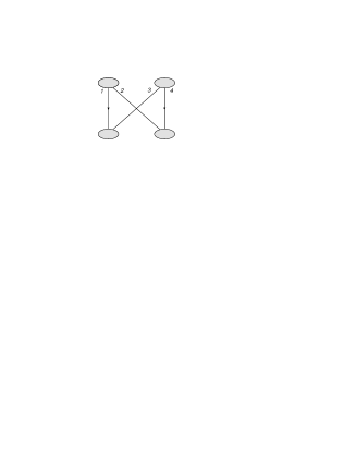
Figure 2: Color redistribution of 4 pomerons

To write down the expression for this diagram it is convenient to make use of the multirapidity formalism for the reggeon dynamics introduced in  [14]. In this formalism resembling the old Gribov technique, each reggeon is assumed to possess its own ”energy” $\epsilon$ apart from its transverse momentum $k$ with the propagator

$$\Delta(\epsilon,k)=\frac{i}{\epsilon+\omega(k)+i0}.$$ (12)

This energy is assumed to be conjugated to the rapidity variable $y$, which is established by the transition of time $t$ to rapidity $y$ according to $it\to y$. At each interaction both energies and transverse momenta are conserved. In this formalism the pomeron with energies and momenta of its two component reggeons $\epsilon_{1},k_{1}$ and $\epsilon_{2},k_{2}$ can be presented as

$${\cal P}(\epsilon_{1},\epsilon_{2};k_{1},k_{2})=\frac{F(E_{12};k_{1},k_{2})}{(\epsilon_{1}+\omega(k_{1})+i0)(\epsilon_{2}+\omega(k_{2})+i0)}$$ (13)

where $E_{12}+\epsilon_{1}+\epsilon_{2}$ is the total pomeron energy. The ”normal” pomeron $P(E_{12},k_{1},k_{2})$ depending on its own energy $E_{12}$ conjugated to its rapidity is given by

$$P(E_{12},k_{1},k_{2})=\frac{F(E_{12};k_{1},k_{2})}{E_{12}+\omega(k_{1})+\omega(k_{2})}.$$ (14)

Now we turn to the diagram in Fig.2. We assume that the two incoming pomerons have their energies $E_{12}$ and $E_{34}$ and the two outgoing pomerons $E_{13}$ and $E_{24}$. The conservation law gives factor

$$2\pi\delta(E_{12}+E_{34}-E_{13}-E_{24})$$

which will be suppressed in the following. Conservation of energy at each pomeron further restricts the reggeon energies to a single energy, say, $\epsilon_{1}$ with the rest determined as follows

$$\epsilon_{2}=E_{12}-\epsilon_{1},\ \ \epsilon_{3}=E_{13}-\epsilon_{1},\ \ \epsilon_{4}=E_{24}-E_{12}+\epsilon_{1}.$$ (15)

The diagram also depends on fixed total momenta of the pomerons $k_{12}=k_{1}+k_{2}$ and so on with $k_{12}+k_{34}=k_{13}+k_{24}$. As a result there is only one independent transverse momentum, say $k_{1}$ and the rest given as

$$k_{2}=k_{12}-k_{1},\ \ k_{3}=k_{13}-k_{1},\ \ k_{4}=k_{34}-k_{13}+k_{1}.$$

So the diagram will be given by the integral over energy $\epsilon_{1}$ and transverse momentum $k_{1}$. Suppressing the latter integration we find

$$D_{B}(E_{12},E_{34},E_{13},E_{24})=\frac{1}{N_{c}^{2}}\int\frac{d\epsilon_{1}}{2\pi}\frac{F_{12}F_{34}F_{13}F_{24}}{(\epsilon_{1}+\omega_{1})(\epsilon_{2}+\omega_{2})(\epsilon_{3}+\omega_{3})(\epsilon_{4}+\omega_{4})},$$ (16)

Here $F_{12}=F(E_{12};1,2)$, for brevity we denote the transverse momenta by just their numbers: $1=k_{1}$ and so on. It is assumed that each $F$ carries factor $\alpha_{c}N_{c}$ which produces the overall factor $1/N_{c}^{2}$. All $\omega$’s are assumed to have a small positive imaginary part. Calculation of the integral over $\epsilon_{1}$ gives

$$I=\int\frac{d\epsilon_{1}}{2\pi}\frac{1}{\epsilon_{1}+\omega_{1}+i0}\,\frac{1}{E_{12}-\epsilon_{1}+\omega_{2}+i0}\,\frac{1}{E_{13}-\epsilon_{1}+\omega_{3}+i0}\,\frac{1}{E_{24}-E_{12}+\epsilon_{1}+\omega_{4}+i0}.$$

$$=-\frac{i}{E_{13}-E_{12}+\omega_{3}-\omega_{2}}\,\Big{\{}\frac{1}{E_{12}+\omega_{1}+\omega_{2}+i0}\,\frac{1}{E_{24}+\omega_{2}+\omega_{4}+i0}$$

$$-\frac{1}{E_{13}+\omega_{1}+\omega_{3}+i0}\,\frac{1}{E_{34}+\omega_{3}+\omega_{4}+i0}\Big{\}}.$$ (17)

In terms of pomerons $P(E;k_{1},k_{2})$ the diagram will be given after the transverse momentum integration of

$$D_{1}(E_{12},E_{34},E_{13},E_{24})=-i\frac{1}{N_{c}^{2}}\Big{(}\frac{1}{2}(E_{12}+E_{34}+E_{13}+E_{24})+\sum_{i=1}^{4}\omega_{i}\Big{)}$$

$$\times P_{12}P_{34}P_{13}P_{24}.$$ (18)

where $P_{12}\equiv P(E_{12};1,2)$ and so on. Passing to dependence on rapidities we have

$$D_{1}(y_{12},y_{34},y_{13},y_{24})=\frac{1}{N_{c}^{2}}\int\frac{dE_{12}dE_{34}dE_{13}dE_{24}}{(2\pi)^{4}}$$

$$\times 2\pi\delta(E_{12}+E_{34}-E_{13}-E_{24})e^{-y_{12}E_{12}-y_{34}E_{34}+y_{13}E_{13}+y_{24}E_{24}}D_{1}(E_{12},E_{34},E_{13},E_{24})$$ (19)

where we discriminate between the incoming and outgoing pomerons, $P_{12},P_{34}$ and $P_{13},P_{24}$ respectively. We introduce the vertex rapidity $y=it$ by presenting

$$2\pi\delta(E_{12}+E_{34}-E_{13}-E_{24})=\int dte^{it(E_{12}+E_{34}-E_{13}-E_{24}}$$

and for each pomeron use

$$\int\frac{dE}{2\pi}P(E,k_{1},k_{2})e^{-tE}=P(t;k_{1},k_{2}),\ \ {\rm with}\ \ P(t;k_{1},k_{2})=0\ \ {\rm at}\ \ t<0$$ (20)

with the subsequent passage $t\to-iy$, in which an extra factor $(-i)$ appears, see [14]).

In this way we ultimately get

$$D_{B}(y_{12},y_{34},y_{13},y_{24})=\frac{1}{N_{c}^{2}}\Big{(}\frac{1}{2}(\partial_{y_{12}}+\partial_{y_{34}}-\partial_{y_{13}}-\partial_{y_{24}})-\sum_{i=1}^{4}\omega_{i}\Big{)}$$

$$\times\int dyP(y_{12}-y;1,2)P(y_{34}-y;3,4)P(y-y_{13};1,3)P(y-y_{24};2,4).$$ (21)

Note that $P(y)$ has a jump at $y=0$. One can put the derivatives inside the integral and rewrite (21) in the form

$$D_{B}(y_{12},y_{34},y_{13},y_{24})=\frac{1}{N_{c}^{2}}\int dy$$

$$\times P(y_{12}-y;1,2)P(y_{34}-y;3,4)\Big{(}\frac{1}{2}\stackrel{{\scriptstyle\leftrightarrow}}{{\partial_{y}}}-\sum_{i=1}^{4}\omega_{i}\Big{)}P(y-y_{13};1,3)P_{24}(y-y_{24};2,4).$$ (22)

So the contribution from the diagram Fig. 1,B splits into two parts

$$D_{B}^{(1)}=\frac{1}{N_{c}^{2}}\frac{1}{2}\int dy\Big{(}P(y_{12}-y;1,2)P(y_{34}-y;3,4)\stackrel{{\scriptstyle\leftrightarrow}}{{\partial_{y}}}P(y-y_{13};1,3)P_{24}(y-y_{24};2,4)\Big{)}$$ (23)

and

$$D_{B}^{(2)}=-\frac{1}{N_{c}^{2}}\sum_{i=1}^{4}\omega_{i}\int dyP(y_{12}-y;1,2)P(y_{34}-y;3,4)P(y-y_{13};1,3)P_{24}(y-y_{24};2,4).$$ (24)

The term $D_{B}^{(2)}$ is infrared divergent due to trajectories $\omega_{i}$. It has order $\alpha_{s}N_{c}$ and is accompanied by factor Y in the diagram, so it has the same order as the diagram in Fig. 1,C to be considered later. In the sum with the latter the infrared divergence will be canceled.

The term $D_{1}^{(1)}$ is infrared finite. To see its order it is convenient to transform it using the BFKL equation (5). The incoming pomeron can be presented via the Green function as

$$P_{12}(y_{12}-y,1,2)=\int d^{4}K^{\prime}\rho_{12}(1,2)(K^{\prime})G(y_{12}-y;K^{\prime},K)\equiv\rho_{12}G(y_{12}-y)$$ (25)

where $K$ combines $k_{1}$ and $k_{2}$, $\rho_{12}$ is the color source and in the second equality $\rho$ and $G(y)$ are considered as operators in the $K$ space, conjugate to the coordinate $z$-space introduced in the Introduction. The Green function satisfies Eq. (5), which is the operatorial notation is

$$\partial_{y}G(y)=1-HG(y)=1-G(y)H.$$ (26)

From this equation we find

$$\partial_{y_{12}}P_{12}(y_{12}-y)=\rho_{12}\delta(y_{12}-y)-P_{12}(y_{12}-y)H_{12}$$ (27)

where the momentum or coordinates are suppressed and it is assumed that Hamiltonian $H_{12}$ acts on them. Similarly for the second incoming pomeron

$$\partial_{y_{34}}P_{34}(y_{34}-y)=\rho_{34}\delta(y_{34}-y)-P_{34}(y_{34}-y)H_{34}.$$ (28)

For the outgoing pomeron we have

$$P_{13}(y-y_{13};1,3)=\int d^{4}K^{\prime}G(y-y_{13};K,K^{\prime})\rho_{(}1,3)(K^{\prime})\equiv G(y-y_{13})\rho_{13},$$ (29)

so that we get in the same way

$$\partial_{y_{13}}P_{13}(y-y_{13})=-\rho_{13}\delta(y-y_{13})+H_{13}P_{13}(y-y_{13})$$ (30)

and

$$\partial_{y_{24}}P_{24}(y-y_{24})=-\rho_{34}\delta(y-y_{24})+H_{24}P_{24}(y-y_{24}).$$ (31)

As a result the contribution $D_{1}^{(1)}$ in its turn splits into two parts. The first part comes from the differentiation of $\delta$ functions in rapidities:

$$D_{B}^{(11)}(y_{12},y_{34},y_{13},y_{24})$$

$$=\frac{1}{N_{c}^{2}}\int dy\Big{\{}\Big{(}\rho(1,2)\delta(y_{12}-y)P(y_{34}-y;3,4)P(y-y_{13};1,3)P(y-y_{24};2,4)+(12)\leftrightarrow(34)\Big{)}$$

$$+\Big{(}\rho(1,3)\delta(y-y_{13})P(y_{12}-y;1,2)P(y_{34}-y;3,4)P(y-y_{24};2,4)+(13)\leftrightarrow(24)\Big{)}\Big{\}}.$$ (32)

The second part includes the Hamiltonian $H$

$$D_{B}^{(12)}(y_{12},y_{34},y_{13},y_{24})=-\frac{1}{N_{c}^{2}}\int dyP(y_{12}-y;1,2)P(y_{34}-y;3,4)$$

$$\times\Big{(}H_{12}+H_{34}+H_{13}+H_{24}\Big{)}P(y-y_{13}1,3)P(y-y_{24};2,4)$$ (33)

Graphically it corresponds to Fig. 3.

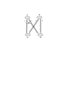
Figure 3: Contribution from the interaction inside the pomerons $P_{12}$. Three others should be added with interactions inside $P_{34}$, $P_{13}$ and $P_{24}$

Restoring the transverse momentum integration and introducing independent momenta for the outgoing pomerons we finally have

$$D_{B}^{(1)}=\frac{1}{2N_{c}^{2}}\int dy\int\frac{d^{2}k_{1}}{(2\pi)^{2}}\prod_{i=1}^{4}\delta^{2}(k_{i}-k^{\prime}_{i})$$

$$\times P(y_{12}-y;1,2)P(y_{34}-y;3,4)\stackrel{{\scriptstyle\leftrightarrow}}{{\partial_{y}}}P(y-y_{13};1^{\prime},3^{\prime})P(y-y_{24};2^{\prime},4^{\prime})\Big{)}$$ (34)

and

$$D_{B}^{(2)}=-\frac{1}{N_{c}^{2}}\sum_{i=1}^{4}\omega_{i}\int dy\int\frac{d^{2}k_{1}}{(2\pi)^{2}}\prod_{i=1}^{4}\delta^{2}(k_{i}-k^{\prime}_{i})$$

$$\times P(y_{12}-y;1,2)P(y_{34}-y;3,4)P(y-y_{13};1^{\prime},3^{\prime})P(y-y_{24};2^{\prime},4^{\prime}).$$ (35)

3.2 Fig. 1.C

The diagram shown in Fig. 1,C includes interaction between reggeons 2 and 3, which with the external pomerons is shown in Fig. 4. Its contribution should be summed with a similar contribution with the gluon interaction between reggeons 1 and 4.

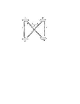
Figure 4: Contribution from the interaction of reggeons 2 and 3. The second diagram should be added with the interaction of reggeona 1 and 4

As before we denote initial total energies as $E_{12}$ and $E_{34}$ and the final energies as $E_{13}$ and $E_{24}$. We again suppress the energy conservation factor $2\pi\delta(E_{12}+E_{34}-E_{13}-E_{24})$. The diagram contains two loops and so energy integrations can be taken over $\epsilon_{1}$ and $\epsilon_{4}$. Energies of the gluons 1, 2, 3 and 4 before the interaction are

$$\epsilon_{1},\ \ E_{12}-\epsilon_{1},\ \ E_{34}-\epsilon_{4},\ \ \epsilon_{4}.$$ (36)

After the interaction gluons 2 and 3 have their energies $E_{24}-\epsilon_{4}$ and $E_{13}-\epsilon_{1}$ respectively and change their momenta $k_{2}\to k^{\prime}_{2}$ and $k_{3}\to k^{\prime}_{3}$. Note that the interaction connects different color configurations with gluons from the projectile forming colorless pairs (1,2) and (3,4) and from the target forming colorless pairs (1,3) and (2,4). As a result the interaction has the opposite sign as compared to the one inside the pomeron  [14]. If the pomeron Hamiltonian is

$$H_{12}=-\omega_{1}-\omega_{2}-V$$ (37)

then the interaction in Fig. 4 is just $-V$.

So in terms of amputated pomerons $F$ the contribution from Fig. 4 before the transverse integrations is

$$D_{C}=i\frac{1}{N_{c}^{2}}\int\frac{d\epsilon_{1}d\epsilon_{4}}{(2\pi)^{2}}$$

$$\times\frac{F_{12}F_{34})F_{13^{\prime}}F_{2^{\prime}4}V(2,3|2^{\prime},3^{\prime})}{(\epsilon_{1}+\omega_{1})(\epsilon_{4}+\omega_{4})(E_{12}-\epsilon_{1}+\omega_{2})(E_{34}-\epsilon_{4}+\omega_{3})(E_{13}-\epsilon_{1}+\omega_{3^{\prime}})(E_{24}-\epsilon_{4}+\omega_{2^{\prime}})}.$$ (38)

Integration over energies factorizes into two integrals:

$$I_{1}=\int\frac{d\epsilon_{1}}{2\pi}\frac{1}{(\epsilon_{1}+\omega_{1}+i0)(E_{12}-\epsilon_{1}+\omega_{2}+i0)(E_{13}-\epsilon_{1}+\omega_{[}3^{\prime}]+i0)}$$

$$=-i\frac{1}{(E_{12}+\omega_{1}+\omega_{2})(E_{13}+\omega_{3^{\prime}})}$$ (39)

and a similar integral over $\epsilon_{4}$ which gives

$$I_{2}=-i\frac{1}{(E_{34}+\omega_{3}+\omega_{4})(E_{24}+\omega_{2^{\prime}}+\omega_{4})}.$$ (40)

So passing to the pomerons we get

$$D_{C}=-i\frac{1}{N_{c}^{2}}V(2,3|2^{\prime},3^{\prime})P(E_{12};1,2)P(E_{34};3,4))P(E_{13};1,3^{\prime})P(E_{24};2^{\prime},4).$$ (41)

The second amplitude $\tilde{D}_{C}$ with the interaction between the gluons 1 and 4 is

$$\tilde{D}_{C}=-i\frac{1}{N_{c}^{2}}V(1,4|1^{\prime},4^{\prime})P(E_{12};1,2)P(E_{34};3,4))P(E_{13};1^{\prime},3)P(E_{24};2,4^{\prime})$$ (42)

Both $D_{C}$ and $\tilde{D}_{C}$ are infrared divergent. Using the fact that the BFKL Hamiltonian is infrared stable as a whole, we can separate the divergence into the reggeon trajectories, presenting (see (37))

$$V(2,3|2^{\prime},3^{\prime})=-H_{23}(2,3|2^{\prime},3^{\prime})-(2\pi)^{4}\delta(2-2^{\prime})\delta(3-3^{\prime})(\omega_{2}+\omega_{3})$$

and

$$V(1,4|1^{\prime},4^{\prime})=-H_{14}(1,4|1^{\prime},4^{\prime})-(2\pi)^{4}\delta(1-1^{\prime})\delta(4-4^{\prime})(\omega_{1}+\omega_{4}).$$

Note that for arbitrary momenta of the outgoing pomerons in the transversal integral $D_{C}$ has to be multiplied by $(2\pi)^{4}\delta^{2}(1-1^{\prime})\delta^{2}(4-4^{\prime})$ and $\tilde{D}_{C}$ has to be multiplied by $(2\pi)^{4}\delta^{2}(2-2^{\prime})\delta^{2}(3-3^{\prime})$. In both cases terms with $\omega_{i}$ acquire the product of all 4 delta-functions between initial and final momenta. Then one finds that the terms with delta-functions cancel with the similar terms in $D_{B}^{(2)}$, Eq. (35). So only the terms with the BFKL Hamiltonian are left and the infrared divergence disappears.

After this cancelation the resulting contribution from the diagrams with one reggeon interaction can be written as

$$D_{1}=D_{C}+\tilde{D}_{C}=i\frac{1}{N_{c}^{2}}P(E_{12};1,2)P(E_{34};3,4)P(E_{13};1^{\prime},3^{\prime})P(E_{24};2^{\prime},4^{\prime})$$

$$\times\Big{(}H(2,3|2^{\prime},3^{\prime})(2\pi)^{4}\delta^{2}(1-1^{\prime})\delta^{2}(4-4^{\prime})+H(1,4|1^{\prime},4^{\prime})(2\pi)^{4}\delta^{2}(2-2^{\prime})\delta^{(}3-3^{\prime})\Big{)}.$$ (43)

Transition to rapidities, as before, will give

$$D_{1}(y_{12},y_{34},y_{13},y_{14})$$

$$=-\frac{1}{N_{c}^{2}}\int dyP(y_{12}-y;1,2)P(y_{34}-y;3,4)P(y-y_{13};1^{\prime},3^{\prime})P(y-y_{24};2^{\prime},4^{\prime})$$

$$\times\Big{(}H(2,3|2^{\prime},3^{\prime})(2\pi)^{4}\delta^{2}(1-1^{\prime})\delta^{2}(4-4^{\prime})+H(1,4|1^{\prime},4^{\prime})(2\pi)^{4}\delta^{2}(2-2^{\prime})\delta^{2}(3-3^{\prime})\Big{)}.$$ (44)

Symbolically it can be written as

$$D_{1}(y_{12},y_{34},y_{13},y_{14})$$

$$=-\frac{1}{N_{c}^{2}}\int dyP(y_{12}-y;1,2)P(y_{34}-y;3,4)\Big{(}H_{23}+H_{14}\Big{)}P(y-y_{13};1^{\prime},3^{\prime})P(y-y_{24};2^{\prime},4^{\prime})$$ (45)

where the relation between different momenta can be seen from Fig. 5.

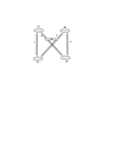
Figure 5: Infrared stable contribution from the interaction between reggeons @ and 3. The second diagram should be added with the interaction of reggeons 1 and 4

4 The quadruple pomeron vertex and action

By definition the quadruple pomeron vertex $\Gamma$ corresponds to a contribution generated by the coupling of four pomeron propagators, that is the Green function $G$, at rapidity $y$ of the structure

$$\int\prod_{i=1}^{4}\frac{d^{2}k_{i}d^{2}k^{\prime}_{i}}{(2\pi)^{4}}G(y_{12}-y;q_{1},q_{2};k_{1},k_{2})G(y_{34}-y;q_{3},q_{4};k_{3},k_{4})(2\pi)^{2}\delta\Big{(}\sum_{i=1}^{4}(k_{i}-k^{\prime}_{i})\Big{)}$$

$$\times\Gamma(k_{1},k_{2};k_{3}k_{4}|k^{\prime}_{1},k^{\prime}_{3};k^{\prime}_{2},k^{\prime}_{4})G(y-y_{13};k^{\prime}_{1},k^{\prime}_{3};q^{\prime}_{1},q^{\prime}_{3})G(y-y_{24};k^{\prime}_{2},k^{\prime}_{4};q^{\prime}_{2},q^{\prime}_{4})$$ (46)

illustrated in Fig. 6. In the vertex pairs of momenta are grouped to correspond to colorless states. We also define it with the extracted $\delta$ function corresponding to conservation f the total momentum. Inspecting our results in the previous section we can identify contributions $D_{B}^{(1)}$ and $D_{1}$ with this structure. In the sum they give the vertex

$$\Gamma(k_{1},k_{2};k_{3}k_{4}|k^{\prime}_{1},k^{\prime}_{3};k^{\prime}_{2},k^{\prime}_{4})=\frac{1}{N_{c}^{2}}\Big{\{}\frac{1}{2}\stackrel{{\scriptstyle\leftrightarrow}}{{\partial_{y}}}\prod_{i=1}^{4}(2\pi)^{2}\delta^{2}(i-i^{\prime})$$

$$-H(2,3|2^{\prime},3^{\prime})(2\pi)^{4}\delta^{2}(1-1^{\prime})\delta^{2}(4-4^{\prime})-H(1,4|1^{\prime},4^{\prime})(2\pi)^{4}\delta^{2}(2-2^{\prime})\delta^{2}(3-3^{\prime})\Big{\}}.$$ (47)

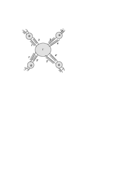
Figure 6: Four pomerons coupled with the quadruple vertex

In accordance with (47) the effective action of pomeron fields acquires new interaction terms

$$S_{I}^{(41)}=\frac{1}{2N_{c}^{2}}\int dy\prod_{i=1}^{4}\frac{d^{2}k_{i}}{(2\pi)^{2}}\Big{\{}\psi^{\dagger}(y,k_{1},k_{2})\psi^{\dagger}(y,k_{3},k_{4})\stackrel{{\scriptstyle\leftrightarrow}}{{\partial_{y}}}\psi(y,k_{1},k_{3})\psi(y,k_{2},k_{4})\Big{\}}$$ (48)

(note that the derivative acts on all field variables in (48)). and

$$S_{I}^{(42)}=\frac{1}{2N_{c}^{2}}\int dy\int\prod_{i=1}^{4}\frac{d^{2}k_{i}d^{2}k^{\prime}_{i}}{(2\pi)^{4}}$$

$$\Big{(}H(2,3|2^{\prime},3^{\prime})(2\pi)^{4}\delta^{2}(1-1^{\prime})\delta^{2}(4-4^{\prime})+H(1,4|1^{\prime},4^{\prime})(2\pi)^{4}\delta^{2}(2-2^{\prime})\delta^{2}(3-3^{\prime})\Big{)}$$

$$\times\psi(y,k_{1},k_{2})\psi(y,k_{3},k_{4})\psi^{\dagger}(y,k^{\prime}_{1},k^{\prime}_{3})\psi^{\dagger}(y,k^{\prime}_{2},k^{\prime}_{4})$$ (49)

One can write down the quasi-classical equations following from $\delta S/\delta\psi=\delta S/\delta\psi^{\dagger}=0$. To do this in the coordinate space one has to Fourier transform $\psi$ and $\psi^{\dagger}$ in (60) taking into account also the corresponding transformation of $H_{23}$ and $H_{14}$. However these general equations have little sense since in applications to the nucleus-nucleus collisions the pomerons have zero total transverse momenta. In this case the equations substantially simplify (see  [5, 8]) and will be studied in the next section. The general, nonforward form of (60), whether in the coordinate or momentum space, is in fact essential only for the study of conformal invariance and calculating loops, the latter task remaining still very remote in future.

5 Forward case

In applications to the nucleus-nucleus scattering and in absence of loops all interacting pomerons have their total transverse momentum equal to zero. So the pomeron wave functions depend on the single transverse variable $r$ or $k$ in the coordinate or momentum spaces. For the forward pomerons it is natural to pass to the so-called semi-amputated pomerons defining in the momentum space

$$\psi(y,k)=k^{2}\phi(y,k),\ \ \psi^{\dagger}(y,k)=k^{2}\phi^{\dagger}(y,k).$$

In terms of these pomeron fields the action with only the triple-pomeron interaction was introduced in  [5, 8].

$$S=S_{0}+S_{3}+S_{E}.$$ (50)

The free action is then

$$S_{0}=\int\frac{dyd^{2}k}{(2\pi)^{2}}\phi^{\dagger}(y,k)K(\stackrel{{\scriptstyle\leftrightarrow}}{{\partial_{y}}}+H)\phi(y,k)$$ (51)

where $H$ is the forward Hamiltonian (4).

$$H(k,-k|k^{\prime},-k^{\prime})=-(2\pi)^{2}\delta^{2}(k-k^{\prime})2\omega(k)-4\alpha_{s}N_{c}\frac{1}{(k-k^{\prime})^{2}},$$ (52)

Momenta $k$ and $k^{\prime}$ are two-dimensional transversal and $K$ is a differential operator in $k$ commuting with $H$

$$K=\nabla_{k}^{2}k^{4}\nabla_{k}^{2}.$$ (53)

Appearance of the operator $K$ in (51) as compared to (2) is due to the transition of the semi-amputated pomerons in the coordinate space to the momentum space.

The interaction part of the action describes splitting and merging of pomerons:

$$S_{I}^{(3)}=\frac{4\alpha_{s}^{2}N_{c}}{\pi}\int\frac{dyd^{2}k}{(2\pi)^{2}}\Big{(}{\phi^{\dagger}}^{2}(y,k)K\phi(y,k)+\phi^{2}(y,k)K\phi^{\dagger}(y,k)\Big{)}.$$ (54)

The external action is

$$S_{E}=-\int\frac{dyd^{2}k}{(2\pi)^{2}}\Big{(}w_{B}(k,)\phi(y,k)\delta(y-Y)+w_{A}(k)\phi^{\dagger}(y,k))\delta(y)\Big{)},$$ (55)

where $w_{A,B}$ as before describe the interaction of the pomerons with the projectile and target. At fixed transverse point $b_{A}$ in the nucleus A coupling $w_{A}(k)$ is supposed to be proportional to the profile nuclear function $T_{A}(b_{A})$ and its dependence on $k$ is determined by the gluon distribution in the nucleon.

Fields $\phi$ and $\phi^{\dagger}$ as well as $w$ are dimensionless. At fixed $b_{A}$ and $b_{B}$ action $S$ is dimensionful: dim$\,S(b_{A},b_{B})=2$. It becomes dimensionless after integration over $b_{A}$ at fixed impact parameter $b$, so that $b_{B}=b_{A}-b$.

Note that in (51) it is assumed that the integration in $y$ goes over the whole axis: $-\infty<y<+\infty$ with the conditions that $\phi(y,k)=0$ at $y<y_{min}+0$ and $\phi^{\dagger}(y,k)=0$ at $y>y_{m}ax=Y$. At $y=0$ and $y=Y$ the piece with $\partial_{y}$ contributes terms proportional to $\delta(y)$ and $\delta(y-Y)$ due to jumps of $\phi$ and $\phi^{\dagger}$.

Turning to the quadruple pomeron interaction we have the same diagrams shown in Fig. 1 B and C which after the cancelation of the terms with $\omega$ give the contributions (34) and (44). Taking $y_{12}=y_{34}=Y$ and $y_{13}=y_{24}=0$ we find for the forward direction

$$D_{B}^{(1)}=\frac{1}{2N_{c}^{2}}\int dy\int\frac{d^{2}k}{(2\pi)^{2}}P_{u}(Y-y,k)P_{u}(Y-y,k)\stackrel{{\scriptstyle\leftrightarrow}}{{\partial_{y}}}P_{l}(y,k)P_{l}(y,k)$$ (56)

and

$$D_{1}=\frac{2}{N_{c}^{2}}\int dy\frac{d^{2}kd^{2}k^{\prime}}{(2pi)^{4}}P_{u}(Y-y,k)P_{u}(Y-y,k^{\prime})P_{l}(y,k)P_{l}(y,k^{\prime})H(k,k^{\prime}|k^{\prime},k).$$ (57)

For clarity we denote the upper and lower pomerons in our figures by subindexes $u$ and $l$ Note that in (57) $H$ is not the forward Hamiltonian:

$$H(k,k^{\prime}|k^{\prime},k)=-(2\pi)^{2}\delta^{2}(k-k^{\prime})2\omega(k)-\frac{2\alpha_{s}N_{c}}{k^{2}{k^{\prime}}^{2}}\Big{(}\frac{k^{4}+{k^{\prime}}^{4}}{(k-k^{\prime})^{2}}-(k+k^{\prime})^{2}\Big{)}.$$ (58)

From these expressions we can read the corresponding quadruple pomeron vertex and action $S_{4}$. From $D_{B}^{(1)}$ we find the vertex

$$\Gamma_{4}^{(1)}=\frac{1}{2N_{c}^{2}})\stackrel{{\scriptstyle\leftrightarrow}}{{\partial_{y}}}$$ (59)

with the contribution to the action

$$S_{4}^{(1)}=\frac{1}{2N_{c}^{2}}\int dy\int\frac{d^{2}k}{(2\pi)^{2}}{\phi^{\dagger}}^{2}(y,k)\stackrel{{\scriptstyle\leftrightarrow}}{{\partial_{y}}}{\phi}^{2}(y,k)=\frac{1}{N_{c}^{2}}\int dy\int\frac{d^{2}k_{1}}{(2\pi)^{2}}({\phi^{\dagger}}^{2}\phi\partial_{y}\phi-\phi^{2}\phi^{\dagger}\partial_{y}\phi^{\dagger}).$$ (60)

For the equations of motion, which for $\phi(y,k)$ is obtained after differentiation $\delta/\delta\phi^{\dagger}$, one gets a contribution

$$\frac{\delta}{\delta\phi^{\dagger}}S_{4}^{(1)}=\frac{2}{N_{c}^{2}}\phi^{\dagger}\partial_{y}\phi^{2}=\frac{4}{N_{c}^{2}}\phi^{\dagger}\phi\partial_{y}\phi$$ (61)

The second contribution to the action from the quadruple pomeron interaction comes from (57)

$$S_{4}^{(2)}=\frac{2}{N_{c}^{2}}\int dy\frac{d^{2}kd^{2}k^{\prime}}{(2\pi)^{4}}\phi(y,k)\phi(y,k^{\prime})\phi^{\dagger}(y,k)\phi^{\dagger}(y,k^{\prime})H(k,k^{\prime}|k^{\prime},k).$$ (62)

The classical equations of motion which follow, multiplied by $(1/2)K^{-1}$ from the left, are

$$\left(\frac{\partial}{\partial y}+H\right)\phi(y,k)+\frac{2\alpha_{s}^{2}N_{c}}{\pi}\Big{(}\phi^{2}(y,k)+2K^{-1}\phi^{\dagger}(y,k)K\phi(y,k)\Big{)}$$

$$+\frac{2}{N_{c}^{2}}K^{-1}\int\frac{d^{2}k^{\prime}}{(2\pi)^{2}}\phi(y,k)\phi^{\dagger}(y,k^{\prime})H(k,k^{\prime}|k^{\prime},k)\phi(y,k^{\prime})$$

$$+\frac{2}{N_{c}^{2}}K^{-1}(\phi^{\dagger}\phi\partial_{y}\phi)=\frac{1}{2}K^{-1}w_{A}(k)\delta(y)$$ (63)

and

$$\left(-\frac{\partial}{\partial y}+H\right)\phi^{\dagger}(y,k)+\frac{2\alpha_{s}^{2}N_{c}}{\pi}\Big{(}{\phi^{\dagger}}^{2}(y,k)+2K^{-1}\phi(y,k)K\phi^{\dagger}(y,k)\Big{)}$$

$$+\frac{2}{N_{c}^{2}}K^{-1}\int\frac{dk^{\prime}}{(2\pi)^{2}}\phi^{\dagger}(y,k)\phi^{\dagger}(y,k^{\prime})H(k,k^{\prime}|k^{\prime},k)\phi(y,k^{\prime})$$

$$-\frac{2}{N_{c}^{2}}K^{-1}(\phi\phi^{\dagger}\partial_{y}\phi^{\dagger})=\frac{1}{2}K^{-1}w_{B}(k)\delta(y-Y).$$ (64)

From the $\delta$-like dependence on $y$ of the external sources it follows that the equations can be taken homogeneous in the interval $0<y<Y$, action of the external sources substituted by the boundary conditions in rapidities

$$\phi(0,k)+\frac{1}{N_{c}^{2}}K^{-1}(\phi^{\dagger}(0)\phi^{2}(0))=\frac{1}{2}K^{-1}w_{A}(k),$$

$$\phi^{\dagger}(Y,k)+\frac{1}{N_{c}^{2}}K^{-1}(\phi(Y){\phi^{\dagger}}^{2}(Y))=\frac{1}{2}K^{-1}w_{B}(k).$$ (65)

We noted in our previous papers that already with $S_{3}$ the equations of motion are no more pure evolution equations, since the initial conditions for $\phi(y)$ and $\phi^{\dagger}(y)$ had to be given at different rapidities, $y=0$ for $\phi$ and $y=Y$ for $\phi^{\dagger}$. Inclusion of quadruple action $S_{4}^{(1)}$ further complicates the situation, since according to (65) the initial conditions now each contain both $\phi$ and $\phi^{\dagger}$.

To see the orders of magnitude of different terms in these equations it is instructive to rescale the pomeron fields $\phi$ and $\phi^{\dagger}$, Hamiltonian and rapidity as

$$\phi\to\frac{\phi}{2\alpha_{s}},\ \ \phi^{\dagger}\to\frac{\phi^{\dagger}}{2\alpha_{s}},\ \ H=\bar{\alpha}\bar{H},\ \ y=\frac{\bar{y}}{\bar{\alpha}}$$ (66)

where $\bar{\alpha}=\alpha_{s}N_{c}/\pi$ Then the equations take the form

$$\frac{\partial\phi(\bar{y},k)}{\partial\bar{y}}=F\{\phi,\phi^{\dagger},\partial_{y}\phi\}$$ (67)

and

$$-\frac{\partial\phi(\bar{y},k)}{\partial\bar{y}}=F^{\dagger}\{\phi,\phi^{\dagger},\partial_{y}\phi^{\dagger}\},$$ (68)

where

$$F=-\bar{H}\phi(\bar{y},k)-\phi^{2}(\bar{y},k)-2K^{-1}\phi^{\dagger}(\bar{y},k)K\phi(\bar{y},k)$$

$$-\frac{1}{2(\bar{\alpha}\pi)^{2}}K^{-1}\int\frac{d^{2}k^{\prime}}{(2\pi)^{2}}\phi(\bar{y},k)\phi^{\dagger}(\bar{y},k^{\prime})\bar{H}(k,k^{\prime}|k^{\prime},k)\phi(\bar{y},k^{\prime})-\frac{1}{2(\bar{\alpha}\pi)^{2}}K^{-1}(\phi^{\dagger}\phi\partial_{y}\phi)$$ (69)

and

$$F^{\dagger}=-\bar{H}\phi^{\dagger}(\bar{y},k)-{\phi^{\dagger}}^{2}(\bar{y},k)-2K^{-1}\phi(\bar{y},k)K\phi^{\dagger}(\bar{y},k)$$

$$-\frac{1}{2(\bar{\alpha}\pi)^{2}}K^{-1}\int\frac{d^{2}k^{\prime}}{(2\pi)^{2}}\phi^{\dagger}(\bar{y},k)\phi(\bar{y},k^{\prime})\bar{H}(k,k^{\prime}|k^{\prime},k)\phi^{\dagger}(\bar{y},k^{\prime})+\frac{1}{2(\bar{\alpha}\pi)^{2}}K^{-1}(\phi\phi^{\dagger}\partial_{y}\phi^{\dagger}).$$ (70)

We observe that the on the right-hand side the free and triple interactions have the same order unity (actually $\bar{\alpha}$ in the original rapidity, which corresponds to the BK equation). The quadruple interaction has the orders $1/\bar{\alpha}^{2}$, which may be smaller or larger as compared with the two first terms depending on the relation between the small $\alpha_{s}$ and large $N_{c}$.

6 Cross-sections

At fixed overall impact parameter $b$ and rapidity $Y$ the nucleus-A-nucleus-B total cross-section is given by

$$\sigma(Y,b)=2\left(1-e^{-T(Y,b)}\right).$$ (71)

In the perturbative QCD the eikonal function $T$ is given by the sum of all connected diagrams constructed of BFKL pomerons, which interact between themselves and with the participant nuclei, so that $T$ is just the action $S$ for fixed $Y$ and $b$

$$T(Y,b)=-\int d_{2}b_{A}d^{2}b_{B}\delta^{2}(b_{A}-b_{B}-b)S(Y,b_{A},b_{B})$$ (72)

In the quasi-classical approximation (without loops) action $S$ is to be calculated from the sum of (51), (54), 60), (62) and(55) with the solutions of evolution Eqs. (63) and (64), $\phi_{cl}(y,k)$ and $\phi^{\dagger}_{cl}(y,k)$.

Using the equations of motion one can somewhat simplify the expression for $S$. Indeed multiplying the first equation by $2K\phi^{\dagger}$, the second one by $2K\phi$, integrating both over $y$ and $k$ and summing the results one obtains a relation

$$2S_{0}+3S_{3}+4S_{4}+S_{E}=0,$$ (73)

which is valid for the classical action, that is, calculated with the solutions of Eqs. (63) and (64). Note that this condition is fulfilled for any form of interactions in $S_{2}$, $S_{3}$ $S_{4}$ and $S_{E}$, since it depends only on the number of field operators in them and hermiticity. Using this relation we can exclude, say, $S_{4}$ from (12) to find

$$S=\frac{1}{4}\Big{(}2S_{0}\{\phi_{cl},\phi^{\dagger}_{cl}\}+S_{I}^{(3)}\{\phi_{cl},\phi^{\dagger}_{cl}\}+3S_{E}\{\phi_{cl},\phi^{\dagger}_{cl}\}\Big{)}.$$ (74)

7 Numerical estimates

As mentioned in our old paper  [8] one can try to find the solution of our problem by two methods. One of them is to solve Eqs. (67) and (68) by iterations. In the simple case when by symmetry $\phi^{\dagger}(y,k)=\phi(Y-y,k)$ in the first iteration one starts from Eq. (67) and solves it for $\phi(y)$ choosing for $\phi(Y-y)$ some simple initial value, typically just zero. Since in this case both the crossed term $2K^{-1}\phi^{\dagger}(y,k)K\phi(y,k)$ and the term coming from $S_{4}$ are both equal to zero, the equation turns out to be the standard BK equation and its solution is just the sum of fan diagrams attached to the projectile. However at the next step one finds non-zero $\phi^{\dagger}(y)$ as $\phi(Y-y)$ from the obtained solution, so that both terms coming from $S_{3}$ and $S_{4}$ become present. Now on the right-hand side there appears a term which itself contains $\partial_{y}\phi$, so that the equation is

$$\partial_{y}\phi=F(\phi^{\dagger},\phi,\partial_{y}\phi).$$ (75)

To solve it we divide the interval $0<y<Y$ in steps $\Delta$ and find at each step

$$\partial_{y}\phi(y+\Delta)=F\Big{(}\phi^{\dagger}(y),\phi(y),\partial_{y}\phi(y)\Big{)},$$ (76)

that is, using $\partial_{y}\phi$ obtained at the previous step on the right-hand side. One expects that with a sufficiently small $\Delta$ the derivative $\partial_{y}\phi$ will not significantly change between steps and one will have good convergence. Solving in this way the equation one once again determines $\phi(y)$ and $\phi^{\dagger}(y)=\phi(Y-y)$ and starts the third iteration of Eq. (67) and so on. If the iteration procedure is convergent one determines the solution $\phi(y,k)$ and $\phi^{\dagger}(y.k)=\phi(Y-y,k)$ together with their derivatives in rapidity. Then one can find the external couplings $w_{A}$ and $w_{B}$ from (65). So in this approach these couplings are not fixed from the start but found after the equations for $\phi$ and $\phi^{\dagger}$ are solved. This circumstance has to be taken into account comparing these results with the pure perturbational calculations in Sec. 3.

Unfortunately, as was mentioned in  [8] this method has a very narrow region of convergence in $A$ and $Y$, which shrinks with the growth of atomic number and rapidity. Without the quadruple interaction for O-O collisions it converges up to rescaled rapidity $\bar{y}=2$, which for $\bar{\alpha}=0.2$ corresponds to rather small actual rapidities less than 5. In attempt to consider higher rapidities and atomic number in  [8] we recurred to another method trying to find the minimum of the action by a direct variational approach choosing some trying functions for $\phi$ and $\phi^{\dagger}$. Even with very primitive trying functions

$$\phi(y=0,k)e^{\Delta y},\ \ \phi^{\dagger}(y=Y,k)e^{\Delta(Y-y)}$$ (77)

with a varying $\Delta$ in  [8] we could find a minimum for the action for very large atomic numbers and rapidities, which lead to reasonable results for the eikonal function and cross-section. Comparison with the exact minimum found by the solution of the equation of motion at rapidities where such solution could be found by interactions showed that the precision of such variational approach was about 20%.

In the present calculations our primary task was to see the influence of inclusion of the quadruple pomeron interaction. $S_{4}$. We considered both methods, the solution of the quasi-classical equations Eqs. (67) and (68) by iterations and the direct variational approach. In both approaches we used the initial wave function which gave the best results in our old iterational solution of (67) and (68)

$$\phi(y=0,k)=\frac{1}{2}a\ln\Big{(}1+\frac{0.2181}{k^{2}}\Big{)},\ \ a=A\sigma_{0}T_{A}(b_{A}),$$ (78)

where $\sigma_{0}=20.8$ mb and $k$ is in GeV/c. This function is very similar in its behavior to the often used Golec-Biernat distribution but is simpler and leads to somewhat larger region of convergence. One can find some details of the calculations of different pieces of the action in Appendix.

In the iterative procedure to solve (67) and (68) we were confronted with a new problem related to the interaction containing the derivative $\partial_{y}$ from $S_{4}^{(1)}$. Its contribution was found to lead to very high values of $\phi(y,k)$ in the infrared region, which prevented iterations already at very small values of $y$. Note that this problem does not exist for the second quadruple interaction coming from $S_{4}^{(2)}$ which admits iterations at all $k$. To overcome this difficulty we had to introduce an infrared cut at the minimal value $k_{min}=\exp\,t_{min}$ for which iterations were possible. It turned out that $t_{min}\simeq-5$. Even with this limitation the iteration procedure was found to be convergent practically in the same region as without $S_{4}$ only when the quadruple interaction was taken very small. Its relative magnitude is determined by factor $1/\bar{\alpha}^{2}$. For O-O collisions at the overall rapidity $Y=2$ the iterative procedure turned out to be convergent only for quite large values of the coupling constant $\bar{\alpha}\geq 1$. In our calculations we took the lowest possible value $\bar{\alpha}=1.1$.

The gluon density at intermediate values of rapidity $0<y<Y$ coming from both colliding nuclei can be determined as  [8]

$$\frac{dxG(x,k)}{d^{2}bd^{2}k}=\frac{N_{c}^{2}}{2\pi^{3}\bar{\alpha}}\Big{(}h(y,k)+h^{\dagger}(y,k)\Big{)},\ \ h(y,k)=k^{2}\nabla_{k}^{2}\phi(y,k).$$ (79)

In our actual calculations we take $b_{A}=b_{B}=0$ and $h^{\dagger}(y,k)=h(Y-y,k)$. In Fig 7 in the upper left panel we show the sum $h(y,k)+h(Y-y,k)$ for $Y=2$, $\bar{\alpha}=1.1$ and $y=0,1/2$ and 1 obtained after converging iterations with the full quadruple interaction $S_{4}$ with the infrared cut. In the upper right panel we show the same sum with only $S^{(2)}_{4}$ taken into account (and without infrared cut). To compare, in the lower panel we show the same quantity obtained by iterations without $S_{4}$.

Figure 7: Gluon density for O-O collisions at $Y=2$ and $\bar{\alpha}=1$ with the total quadruple interaction $S_{4}$ (upper left panel), with only $S_{4}^{(2)}$ and without infrared cut (upper right panel) and without the quadruple pomeron interaction (lower panel)

A more illustrative comparison is done in Fig. 8. One observes first of all that at small momenta the contribution from the derivative coupling $S_{4}^{(1)}$ blows up, which only exhibits the region of bad convergence. One cannot trust the obtained values of the gluon density in this boundary region. One rather expects the true density to behave roughly as with only $S_{4}^{(2)}$, the contribution from $S_{4}^{(1)}$ only slightly lowering the density, as one can conclude from the figures at momenta immediately before the peak. At the physically important momenta in the region of the peak itself and higher the contribution from the quadruple interaction turned out to be very small due to the assumed high value of $\bar{\alpha}$.

Figure 8: Gluon densities for O-O collisions at $Y=2$ and $\bar{\alpha}=1$ with and without the quadruple pomeron interaction $S_{4}=S_{4}^{(1)}+S_{4}^{(2)}$ at intermediate rapidities $y=0,0.5$ and 1.

The last conclusion is confirmed by the calculation of the eikonal function. In Fig 9 we present the eikonal at ${\bf b}=0$ for $Y=2$, which is obtained from the full action (74) with the solution of equations (67) and (68)after integration over all $b_{A}=b_{B}$. The difference between the present and absent $S_{4}$ is smaller than 1% (and cannot be shown in the plot).

Figure 9: Eikonal $T(0)$ for central O-O collisions at $Y=2$ with the quadruple pomeron interaction $S_{4}$

To conclude with the iterative solution of the quasi-classical equations for the fields, we kave found that it turns out to be dangerous in the infrared region. Probably the equations, being highly non-linear possess solutions of a different type, which avoid these difficulties but cannot be found by iterations.

Passing to direct variational search for the minimum of the action, we recall that without the quadruple interaction one always found the minimum using the trying function (77) with a variable $\Delta$. Now we repeat this exercise with the quadruple interaction included. We drop the infrared cut and take a more reasonable value of $\bar{\alpha}=0.2$, which of course substantially enhances the quadruple interaction. We find that inclusion of $S_{4}$ allows to find the minimum of the action up to rescaled rapidities 5 that is up to natural rapidities 25 but not to higher rapidities. So $S_{4}$ leads to certain restriction on the rapidity range, which however is physically not so bad. To simplify calculations we choose to calculate the action in the approximation of a constant $T_{A}(b_{A})$ for each nucleus and afterwards obtained the eikonal function T(b) integrating the action in the overlap area of the collision depending on the impact parameter $b$. The obtained eikonal for central O-O collisions $T(0)$ is illustrated in Fig 10 (lower curve). To compare we also present $T(0)$ for the case without $S_{4}$ (upper curve). One observes that inclusion of the quadruple interaction substantially reduces the central eikonal. Still the eikonal remains very large numerically. As a result the total O-O cross-section is practically the same with or without $S_{4}$ and with our parametrization equals 151 fm².

Figure 10: Eikonal $T(0)$ for central O-O collisions obtained by the variational approach, with the quadruple pomeron interaction $S_{4}$ (lower curve) and without it (upper curve)

8 Conclusion

We have derived the quadruple pomeron interaction in the lowest order, which is essential in the interaction of nuclei between themselves. It consists of two terms, one with the derivative in rapidity and the other with the BFKL interaction between the pair of pomerons. Both are infrared safe. Their relative order to the triple pomeron interaction is $1/(\alpha_{s}N^{2})$. So the quadruple interaction is much smaller for fixed $\alpha_{s}$ and large number of colors. However in the opposite case with fixed $N_{c}$ and small coupling constant it may become comparable or even greater than the currently used triple interaction. Illustrative and very approximate calculations of the O-O cross-sections with the quadruple interaction together with the triple one and quite large $\bar{\alpha}=1$ showed instability of the iterative procedure in the infrared region but a workable variational approach. We find a noticeable damping of the gluon density at small momenta, although at momenta greater than 1 GeV/c the change is quite small. In the variational approach one finds quite a substantial fall of the eikonal function at all impact parameters due to the quadruple interaction. More precise calculations of the AA collisions are needed to make a final conclusion of the importance of the quadruple interaction for the actual processes.

9 Appendix. Some details of the calculation

We use the logarithmic variable $t$ putting $k=\exp(t)$ where $k$ is measured in units provided by the initial condition $\phi(y,k)_{y=0}=\phi_{0}(k)$. Integration over $k$ transforms as

$$\int\frac{d^{2}k}{(2\pi)^{2}}=\frac{1}{2\pi}\int_{t_{min}}^{t_{max}}k^{2}dt.$$

The integral was done by the Simpson numerical integration in $n=400$ points. Without infrared cut satisfactory results were achieved for $t_{min}=-20$, $t_{max}=+20$. The infrared cut needed for iterations with $S_{4}^{(1)}$ was taken $t_{min}=-5$.

9.1 Equation

The equation to solve can be rewritten in the form

$$\frac{\partial\phi}{\partial y}=+T_{0}+T_{3}^{(1)}+T_{3}^{2)}++T_{4}^{(1)}+T_{4}^{(2)}+T_{E},$$ (80)

where the common arguments are $(y,k)$ and terms $T_{0}$, $T_{3}^{(1,2)}$, $T_{4}^{(1,2)}$ and $T_{4}$ come from the parts $S_{0}$, $S_{3}$, $S_{4}$ and $S_{E}$ of the action. Suppressing the common argument $y$ where it is possible, we have

$$T_{0}(k)=-\int\frac{d^{2}k_{1}}{4\pi^{2}}H(k,k_{1}|k,k_{1})\phi(k_{1}).$$ (81)

After angular integration and passing to the integration variable $t_{1}$

$$T_{0}(k)=\bar{\alpha}\int dt_{1}\Big{(}B(k,k_{1})\phi(k_{1})-A(k,k_{1})\phi(k)\Big{)},$$ (82)

where

$$B(k,k_{1}=2\frac{k_{1}^{2}}{|k^{2}-k_{1}^{2}|},\ \ A(k,k_{1})=2k^{2}\Big{(}\frac{1}{|k^{2}-k_{1}^{2}|}-\frac{1}{\sqrt{k^{2}+4k_{1}^{2}}}\Big{)}.$$ (83)

From $S_{3}$ we have two terms

$$T_{3}^{(1)}(k)=-\frac{2\alpha_{s}^{2}N_{c}}{\pi}\phi^{2}(k),$$ (84)

$$T_{3}^{(2)}(k)=\frac{4\alpha_{s}^{2}N_{c}}{\pi}K^{-1}\phi^{\dagger}(k)K\phi(k).$$ (85)

Operator $K^{-1}$ is nonlocal with the kernel [5, 8]

$$K^{-1}(k,k_{1})=\frac{\pi}{2}\frac{1}{k_{>}^{2}}\Big{(}\ln\frac{k_{>}}{k_{,}}+1\Big{)}$$ (86)

where $k_{>}(k_{<})$ is the greater(smaller) of momenta $k,k_{1}$.

So after angular integration we get

$$T_{3}^{(2)}(k)=-\frac{2\alpha_{s}^{2}N_{c}}{\pi}\Big{\{}\int_{-\infty}{t}dt_{1}e^{-2z}\phi^{\dagger}_{2}(k_{1})\Big{(}(z+1)\phi_{2}(k_{1})-2\phi_{1}(k_{1})\Big{)}$$

$$+\int_{t}^{+\infty}dt_{1}\phi^{\dagger}_{2}(k_{1})\Big{(}(1-z)\phi_{2}(k_{1})+2(2z-1)\phi_{1}(k_{1})-4z\phi(k_{1})\Big{)}\Big{\}},$$ (87)

where $z=t-t_{1}$, $\phi_{1}=(\partial/\partial t)\phi$, $\phi_{2}=(\partial/\partial t)^{2}\phi$.

The two quadruple interaction terms are

$$T_{4}^{(1,2)}(k)=-\frac{2}{N_{c}^{2}}\int\frac{d^{2}k_{1}}{(2\pi)^{2}}K^{-1}(k,k_{1})\chi^{(1,2)}(k_{1}),$$ (88)

where

$$\chi^{(1)}(k)=\phi^{\dagger}(k)\phi(k)\partial_{y}\phi(k),$$ (89)

and

$$\chi^{(2)}(k)=\phi(k)\int\frac{d^{2}k_{1}}{4\pi^{2}}\phi^{\dagger}(k_{1})H(k,k_{1}|k_{1},k)\phi(k_{1})$$ (90)

Doing the angular integration and passing to integration variable $t_{1}$ we obtain, similarly to (82):

$$\chi^{(2)}(k)=-\bar{\alpha}\phi(k)\int dt_{1}\Big{(}B_{1}(k,k_{1})\phi(k_{1})\phi^{\dagger}(k_{1})-A(k,k_{1})\phi(k)\phi^{\dagger}(k)\Big{)},$$ (91)

where $A$ is the same as in (83) and

$$B_{1}(k,k_{1})=\frac{k^{4}+k_{1}^{4}}{k^{2}}.$$ (92)

Finally the external term is

$$T_{E}(y,k)=\frac{1}{2}K^{-1}w_{A}(k)\delta(y).$$ (93)

To obtain our final expressions for calculation we first rescale $\phi$, $\phi^{\dagger}$ and $y$ as indicated in (66) and afterwards divide by $2\alpha_{s}\bar{\alpha}$. Then the coefficients in $T_{0}$ and $T_{3}^{(1)}$ turn to unity and in $T_{3}^{(2)}$ to 1/2. The coefficient in $T_{4}$ is divided by $4\alpha_{s}^{2}\bar{\alpha}$. so we get for the total coefficient $1/(2\pi^{2}\bar{\alpha}^{2})$. Finally the rescaling of $y$ produces factor $\bar{\alpha}$ in $T_{E}$ so that the coefficient becomes equal to $\alpha_{s}$.

As a result after rescaling equation (63) takes the form (80) with rescaled $y$ and $T_{0},...T_{E}$ which are explicitly

$$T_{0}(k)=\int dt_{1}\Big{(}B(k,k_{1})\phi(k_{1})+A(k,k_{1})\phi(k)\Big{)},$$ (94)

$$T_{3}^{(1)}(k)=-\phi^{2}(k),$$ (95)

$$T_{3}^{(2)}(k)=-\frac{1}{2}\Big{\{}\int_{-\infty}^{t}dt_{1}e^{-2z}\phi^{\dagger}_{2}(k_{1})\Big{(}(z+1)\phi_{2}(k_{1})-2\phi_{1}(k_{1})\Big{)}$$

$$+\int_{t}^{+\infty}dt_{1}\phi^{\dagger}_{2}{k_{1})\Big{(}(1-z)\phi_{2}(k_{1})+2(2z-1)\phi_{1}(k_{1}}-4z\phi(k_{1})\Big{)}\Big{\}},$$ (96)

where $z=t-t_{1}$,

$$T_{4}^{(1,2)}(k)=\frac{1}{2\pi^{2}\bar{\alpha}^{2}}\,\frac{1}{4}\int dt_{1}k_{1}^{2}\frac{1}{k_{>}^{2}}(t_{>}-t_{<}+1)\chi^{(1,2)}(k_{1}),$$ (97)

where $k>,t>$ and $k<,t<$ are the larger and small of $k,t$ and $k_{1},t_{1}$ and the rescaled $\chi$ are given by (89) and (90) without coefficient $\bar{\alpha}$. Finally

$$T_{E}(y,k)=\frac{\pi}{N_{c}}K^{-1}w_{A}(k)\delta(\bar{y}).$$ (98)

From the equation at $y=0$ it follows that $\phi(y=0,k)=\alpha_{s}K^{-1}w_{A}(k)$, so that

$$\frac{1}{2}K^{-1}w_{A}(k)=\frac{1}{2\alpha_{s}}\phi(y=0,k),\ \ {\rm or}\ \ w_{A}(k)=\frac{1}{\alpha_{s}}K\phi(y=0,k).$$ (99)

9.2 Action

The action is given by Eqs. (51), (54), (60), (62) and (55) and is a sum

$$S=S_{0}+S_{3}+S_{4}+S_{E}$$ (100)

Here we present it in the explicit form.

We begin with $S_{0}$ which is given by (51). It contains two terms: one with the derivative $S_{0}^{(1)}$ and the second $S_{0}^{(2)}$ with $H$. We split operator $K$ into the product $K=L^{\dagger}L$. In the logarithmic variable $t$ one finds $L=\partial^{2}/\partial t^{2}$. So after the angular integration we get the part $S_{0}^{(1)}$

$$S_{0}^{(1)}=\frac{1}{2\pi}\int_{0}^{Y}dy\int dtk^{2}\Big{(}\phi^{\dagger}_{2}(y,k)\frac{\partial\phi_{2}(y,k)}{\partial y}-\phi_{2}(y,k)\frac{\partial\phi^{\dagger}(y,k)}{\partial y}\Big{)}.$$ (101)

where we again denoted $\phi_{2}=\partial^{2}\phi/\partial t^{2}$. The integration over $y$ is originally performed in the region $-\infty<y<+\infty$ and so takes into account the jumps at $y-0$ and $y=Y$. Contribution from these jumps gives the boundary term

$$S_{0}^{(b)}=\frac{1}{\pi}\int dtk^{2}\phi^{\dagger}_{2}(0,k)\phi_{2}(0,k).$$ (102)

where we have taken into account that $\phi^{\dagger}(0)=\phi(Y)$, The second term is

$$S_{0}^{(2)}=\frac{\bar{\alpha}}{\pi}\int dtdt_{1}k^{2}\phi^{\dagger}_{2}(y,k)\Big{(}B(k,k_{1})\phi_{2}(y,k_{1})+A(k,k_{1})\phi_{2}(y,k)\Big{)}.$$ (103)

Here and in the following $k_{1}=\exp t_{1}$.

In $S_{3}$ both terms give the same contributions due to the assumed relation $\phi^{\dagger}(y)=\phi(Y-y)$ So

$$S_{3}=\frac{8\alpha_{s}^{2}N_{c}}{\pi}\int dy\frac{d^{2}k}{4\pi^{2}}L\phi^{\dagger}(y,k)L\phi^{2}(y,k)$$

$$=\frac{8\alpha_{s}^{2}N_{c}}{\pi^{2}}\int dydtk^{2}\phi^{\dagger}_{2}(y,k)\Big{(}\phi_{2}(y,k)\phi(y,k)+\phi_{1}^{2}(y,k)\Big{)}.$$ (104)

Next

$$S_{4}^{(1)}=\frac{1}{\pi N_{c}^{2}}\int dy\int dtk^{2}{\phi^{\dagger}}^{2}\phi\partial_{y}\phi.$$ (105)

Presence of the derivative $\partial_{y}$ leads to the contribution from the jumps at $y=0$ and $y=Y$ and generates a new boundary term

$$S_{4}^{(b)}=\frac{1}{2\pi N_{c}^{2}}\int dtk^{2}{\phi^{\dagger}}^{2}(0,k)\phi^{2}(0,k).$$ (106)

The second part is

$$S_{4}^{(2)}=\frac{\bar{\alpha}}{\pi N_{C}^{2}}\int dydtdt_{1}k^{2}\phi(k)\phi^{\dagger}(k)\Big{(}B_{1}(k,k_{1})\phi(k_{1}\phi^{\dagger}(k_{1})-A(k,k_{1})\phi(y,k)\phi^{\dagger}(y,k)\Big{)}.$$ (107)

Finally

$$S_{E}=\frac{1}{\pi}\int dtk^{2}w_{A}(k)\phi^{\dagger}(0,k),$$ (108)

where $w_{A}$ is given by (99).

References

• [1] J.Β Jalilian-Marian, A.Β Kovner, A.Β Leonidov and H.Β Weigert Nucl.Β Phys.Β B504 (1997) 415; Phys.Β Rev.Β D 59 (1999) 014014; E.Β Iancu, A.Β Leonidov, L.Β McLerran, Nucl.Β Phys.Β A 692 (2001) 583; E. Iancu, A. Leonidov, L. McLerran, Phys.Β Lett.Β B 510 (2001) 133; E.Β Ferreiro, E.Β Iancu, A.Β Leonidov and L.Β McLerran, Nucl.Β Phys.Β A 703 (2002) 489; H.Β Weigert, Nucl.Β Phys.Β A 703 (2002) 823.
• [2] L.N.Lipatov, Nucl. Phys. B 452 (1995) 369; Phys. Rep., 286 (1997) 131
• [3] I.Β Balitsky, Nucl.Β Phys.Β B 463 (1996) 99.
• [4] Y.Β V.Β Kovchegov,Phys.Β Rev.Β D 60 (1999) 034008;ibid61 (2000) 074018.
• [5] M.A,Braun, Phys. lett. B 483 (2000) 115
• [6] M.A.Braun, Phys. Lett. B 632 (2006) 297
• [7] M.A.Braun. Eur. Phys. J. C 48 (2006) 511
• [8] M.A.Braun, Eur. Phys. J. C 33 (2004) 113
• [9] S. Bondarenko, L.Motyka,Phys. Rev, D 75 (2007) 114015
• [10] S. Bondarenko, M.A.Braun, Nucl. Phys. A 799 (2008) 151
• [11] K.Dusling, F. Gelis, T. Lappi, R. Venugopalan, Nucl Phys. A 836 (2010) 159.
• [12] S. Bondarenko, L. Motyka, A.H.Mueller, A.I.Shoshi, B.W. Xiao, Eur. Phys. J. C 50 (2007) 593.
• [13] M.A. Braun, G.P.Vacca, Eur. Phys. J. C 50 (2007) 857.
• [14] M.A.Braun, Eur. Phys. J. C 73 (2013): 2418
• [15] J.Bartels, L.N.Lipatov, G.P.Vacca, Nucl. phys, 706 (2005) 391
• [16] M.A.Braun, Eur. Phys. J. C 70 (2010) 73