Semiparametric bivariate extreme-value copulas

Abstract

Extreme-value copulas arise as the limiting dependence structure of component-wise maxima. Defined in terms of a functional parameter, they are one of the most widespread copula families due to their flexibility and ability to capture asymmetry. Despite this, meeting the complex analytical properties of this parameter in an unconstrained setting remains a challenge, restricting most uses to models with very few parameters or nonparametric models. Focusing on the bivariate case, we propose a novel semiparametric approach. Our procedure relies on a series of transformations, including Williamson’s transform and starting from a zero-integral spline. Without further constraints, wholly compliant solutions can be efficiently obtained through maximum likelihood estimation, leveraging gradient optimization. We successfully conducted several experiments on simulated and real-world data. Our method outperforms another well-known nonparametric technique over small and medium-sized samples in various settings. Its expressiveness is illustrated with precious data gathered by the gravitational wave detection LIGO and Virgo collaborations.

1 Introduction

A copula $C$ is an extreme-value copula (EVC) if it is the weak limit of copulas emerging from component-wise maxima [28]. In the bivariate case, EVCs can be expressed as

$$C(u,v)=\exp\left\{\log(uv)A\left[\frac{\log(u)}{\log(uv)}\right]\right\}\,,\ \text{for}\ u,v\in(0,1)^{2}\,,$$

where $A:[0,1]\longrightarrow\mathbb{R}$, known as the Pickands function (PF), satisfies the following two constraints:

1. $\max\{t,1-t\}\leq A(t)\leq 1$, for all $t\in[0,1]$.

2. $A$ is convex.

The segments making the lower bound for $A$ are called the support lines of the PF. Fig. 1(a) shows the PF geometry.

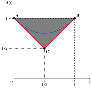
(a) Pickands geometry

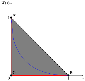
(b) 2-monotone geometry

Fig. 1: On the left, PF geometry. The admissible region for its graph appears in grey. The support lines show in red. An example of PF, namely $A(t)=t^{2}-t+1$, is drawn in blue. On the right, the geometry of a 2-monotone function derived from a PF through an affine transformation mapping $\mathbf{A}$, $\mathbf{B}$ and $\mathbf{C}$ to $\mathbf{A}^{\prime}$, $\mathbf{B}^{\prime}$ and $\mathbf{C}^{\prime}$. The transformed version of the PF on the left, $W(x)=x-2\sqrt{x}+1$, is drawn in blue. The graph of the function $W$ ranges from $\mathbf{A}^{\prime}$ to $\mathbf{B}^{\prime}$ and never crosses the dashed line segment between these two points.

The PF constraints are not inherently satisfied by conventional approximation methods. Thus, most EVC modelling depends on well-known one-parameter symmetrical families, like in Table 1. [38]’s device allows obtaining asymmetrical EVCs from the latter, somewhat extending the applicability of parametric models [38, 19]. If $A$ is a PF, given $\alpha,\beta\in(0,1]$, the following will also be a PF:

$$A_{\alpha,\beta}(t)=(1-t)(1-\alpha)+t(1-\beta)+w\ A\left(\frac{t\beta}{w}\right)\,,$$ (1)

where $w=(1-t)\alpha+t\beta$. Nonparametric methods are currently the only alternative.

Family	$A_{\theta}(t)$	$\theta$ range
Gumbel	$\left[t^{\theta}+(1-t)^{\theta}\right]^{1/\theta}$	$[1,\infty)$
Galambos	$1-\left[t^{-\theta}+(1-t)^{-\theta}\right]^{-1/\theta}$	$(0,\infty)$

Table 1: Main one-parameter EVC families [37]. The above families are symmetrical. [38]’s procedure provides a means for introducing asymmetry.

Related work

[55] provide a comprehensive review of EVCs [55]. In general, nonparametric models demonstrate greater flexibility than parametric ones. Parametric models using [38]’s device perform well against nonparametric ones in dimensions higher than two and with mild asymmetry.

One of the first estimators for the PF was proposed by [46] in bivariate survival analysis [46]. However, [46]’s method produces almost surely [35] non-convex PFs over $[0,1]$. [46] himself proposed in [46] to use the greatest convex minorant of the original estimator, which remains one of the most practical and efficient approaches.

Perhaps the most widespread nonparametric method is due to [9] [9], from which it borrows its name CFG. They observe that, given a random sample $\{(U_{i},V_{i})\}_{i=1}^{n}$ from an EVC with PF $A$, the transformation $Z_{i}=\log U_{i}/\log(U_{i}V_{i})$ is distributed according to the cumulative distribution function (CDF)

$$H(z)=z+z(1-z)\frac{A^{\prime}(z)}{A(z)}\,.$$ (2)

One can empirically estimate $H$ with some $\tilde{H}$ and solve (2) for an estimator

$$\tilde{A}(t)=\exp\left\{\int_{0}^{t}\frac{\tilde{H}(z)-z}{z(1-z)}\ dz\right\}\,.$$ (3)

The estimator $\tilde{A}$ is not convex in general either. [35] propose two modified versions of the CFG that satisfy the convexity constraint [35].

Most estimation methods until the early 2010s are variants of either [46]’, CFG or both [55]. More recent advances have focused on polynomials and splines. For instance, [30] study the conditions under which a polynomial, expressed in Bernstein form, is a PF [30]. [42] use Bernstein-Bézier polynomials to enforce some PF constraints [42]. [13] use constrained quadratic smoothing B-splines to develop a compliant PF in a nonparametric fashion using the R cobs package [13].

Previously, [18] had introduced a compliant nonparametric estimator requiring constrained optimization and targeting an equivalent definition of PFs [18]. The PF can be expressed [30] as

$$A(t)=\int_{0}^{1}\max\{t(1-z),z(1-t)\}\ d\mathcal{H}(z)\,,$$

where $\mathcal{H}$ is the so-called spectral measure on $[0,1]$: a finite measure satisfying $\int_{0}^{1}z\ d\mathcal{H}(z)=1$. Under absolute continuity of $A^{\prime}$ [30], $\mathcal{H}$ admits a decomposition

$$\mathcal{H}(B)=\mathcal{H}_{0}\mathbf{1}_{B}(0)+\int_{B}\eta(z)\ dz+\mathcal{H}_{1}\mathbf{1}_{B}(1)\,,$$ (4)

where $\mathbf{1}_{B}$ denotes the indicator function on $B$, $\eta=A^{\prime\prime}$ almost everywhere on $(0,1)$, $\mathcal{H}_{0}=1+A^{\prime}(0^{+})$ and $\mathcal{H}_{1}=1-A^{\prime}(1^{-})$.

The concept of Williamson’s transform has recently irrupted in copula theory [5]. [44] employ it in their study of $d$-monotone Archimedean generators [44, 45]. [11] also use it to model multivariate Archimax copulas [11]. Even though they do not consider it in their work, [21] introduce a subclass of Archimedean copulas called Lorenz copulas, where Williamson’s transform could play a crucial role in estimation, as we later specify.

Goals

Some accepted methods fail to meet all the constraints required by the PF, even in the bivariate case [55]. Semiparametric approaches, like the one introduced by [32] for Archimedean copulas [32], have not been explored in the context of EVCs.

The research community is currently focusing on $n$-variate extensions [29]. However, a more flexible and sound construction is missing in the bivariate context. The work by [37] suggests that the bivariate EVC family is not as narrow, especially under asymmetry [37]. Our method will thus exclusively focus on the bivariate setting.

The semiparametric procedure we introduce here offers the following advantages over state-of-the-art methods:

• Built-in PF constraint compliance, mapping any $\bm{\theta}\in\mathbb{R}^{d}$, for $d$ large, to some PF $A_{\bm{\theta}}$ ranging in a broad spectrum of dependence strengths and asymmetries.

• Optimization of $\bm{\theta}$ via maximum likelihood estimation (MLE), taking the most advantage of each observation, even in small samples.

• Ability to penalize model complexity during the optimization process, especially for large $d$, reducing overfitting and opening opportunities for Bayesian analysis.

The approach by [13] [13], also focusing on the bivariate case, allows for a large $d$, but does not retain control over the domain of $\bm{\theta}$. Given a sample $\{(U_{i},V_{i})\}_{i=1}^{n}$ from an EVC with PF $A$, the random variables $(Z_{i},T_{i})$, where $Z_{i}=\log U_{i}/\log(U_{i}V_{i})$, $T_{i}=\log\hat{C}(U_{i},V_{i})/\log(U_{i}V_{i})$, and $\hat{C}$ is the empirical estimate of $C$, lie close to $A$’s graph. Then one can perform a constrained B-splines regression on those points. However, the estimation procedure chooses the coordinates to satisfy the PF constraints since not all parameters would be valid. Hence, their method lacks a proper structure, falling into the nonparametric category. Difficulties are bound to appear with small samples after relying on the empirical copula $\hat{C}$ and a regression approach.

Outline

We introduce in Section 2 our semiparametric method. We formally construct and estimate a large subclass of EVCs and explore their properties. A includes all the proofs. We then test our method on a simulation study (SS) and a real-world case study in Section 3. Section 4 provides further comments on our method’s performance and general possibilities. Finally, we offer some concluding remarks in Section 5.

2 Method

In the following sections, we will cover (i) the construction of a new semiparametric EVC, (ii) some of its properties, (iii) estimation algorithms, (iv) simulation, and (v) a possible solution to one of its limitations.

2.1 Construction

A copula arising from our construction will be called a semiparametric bivariate extreme-value copula (SBEVC). We will also refer to our method as SBEVC. The construction of SBEVCs encompasses several steps. The following sections will go through them from our PF goal to a coordinates vector. In each stage, the complexity of the parameter decreases, from an infinite-dimensional functional parameter with stringent constraints to an arbitrary $\bm{\theta}\in\mathbb{R}^{d}$. That is not the natural order in the estimation phase, but it constitutes the safest path to weigh the sacrifices we make along the way. Notwithstanding, we briefly summarize the journey in its final form:

1. Given $\bm{\theta}\in\mathbb{R}^{d}$, we build a zero-integral B-spline (ZBS) $p_{\bm{\theta}}$ defined in $[0,1]$.

2. We apply to $p_{\bm{\theta}}$ the inverse centred log-ratio (CLR) transformation to obtain a probability density function (pdf) $f_{\bm{\theta}}$ supported on $[0,1]$.

3. We integrate $f_{\bm{\theta}}$ using the Williamson transform (WT) to obtain a 2-monotone function $W_{\bm{\theta}}$ supported on $[0,1]$.

4. We affinely transform $W_{\bm{\theta}}$ to arrive at the PF $A_{\bm{\theta}}$, as depicted in Fig. 1.

2.1.1 Affine transformation

The support lines of the PF resemble a pair of coordinate axes if rotated and scaled. Let $M$ be the unique 2-dimensional affine transformation mapping $(0,1)$, $(0,0)$ and $(1,0)$ to $(0,1)$, $(1/2,1/2)$ and $(1,1)$, respectively. $M$ and $M^{-1}$ take the form

$$M(x,w)=\frac{1}{2}\begin{pmatrix}1+x-w\\ 1+x+w\end{pmatrix}\,,$$ (5)

$$M^{-1}(t,a)=\begin{pmatrix}t+a-1\\ a-t\end{pmatrix}\,.$$ (6)

Under certain conditions, the inverse mapping $M^{-1}$ transforms the graph of a PF, $\left\{(t,A(t))\ |\ t\in[0,1]\right\}$, into the graph of a 2-monotone function $W$ defined on $[0,1]$ and satisfying $W(0)=1$ and $W(1)=0$. Here, 2-monotone stands for non-increasing and convex [44, 11]. Fig. 1 shows the transition from one to the other. Note that for a twice differentiable function $W$ with the above boundary constraints, 2-monotonicity is equivalent to $W^{\prime}(x)\leq 0$ and $W^{\prime\prime}(x)\geq 0$, for all $x\in(0,1)$.

Proposition 1.

prop:A-W-equivalence Let all the upcoming functions be twice differentiable on $(0,1)$. By means of (5) and its inverse (6), there is a one-to-one correspondence between PFs $A$ satisfying $A(t)>1-t$, for all $t\in(0,1/2]$, and 2-monotone functions $W$ defined on $[0,1]$ and satisfying $W(0)=1$, $W(1)=0$. Namely, $A$ can be obtained from $W$ as

$$\left\{\begin{aligned} t(x)&=\frac{1}{2}\left(1+x-W(x)\right)\\ A(t(x))&=\frac{1}{2}\left(1+x+W(x)\right)\end{aligned}\right.$$ (7)

and conversely, $W$ from $A$, as

$$\left\{\begin{aligned} x(t)&=t+A(t)-1\\ W(x(t))&=A(t)-t\end{aligned}\right.\,,$$ (8)

where both $t(x)$ and $x(t)$ are automorphisms of $[0,1]$. Moreover,

$$A^{\prime}(t(x))=\frac{1+W^{\prime}(x)}{1-W^{\prime}(x)}\,,$$ (9)

$$A^{\prime\prime}(t(x))=\frac{4\ W^{\prime\prime}(x)}{\left(1-W^{\prime}(x)\right)^{3}}\,,$$ (10)

and

$$W^{\prime}(x(t))=\frac{A^{\prime}(t)-1}{A^{\prime}(t)+1}\,,$$ (11)

$$W^{\prime\prime}(x(t))=\frac{2\ A^{\prime\prime}(t)}{\left(1+A^{\prime}(t)\right)^{3}}\,.$$ (12)

Remark 1.

We do not need the smoothness assumption in prop:A-W-equivalence in either direction. We can argue that affine transformations map convex epigraphs into convex epigraphs. Hence, the convexity of $A$ is equivalent to that of $W$. Nonetheless, differentiability is a convenient requirement for our construction.

Example 1.

ex:polynomial-pickands-W Elaborating on Fig. 1, plugging $A(t)=t^{2}-t+1$ into (8) yields the $W(x)=x-2\sqrt{x}+1$ we see in Fig. 1(b).

Example 2.

ex:power-W-family The family of functions $W_{\theta}(x)=(1-x)^{\theta}$, where $\theta\in[1,\infty)$, meet the conditions in prop:A-W-equivalence and thus produce EVCs.

A $W$ function like the one defined in prop:A-W-equivalence induces a spectral measure (4) by means of

$$\eta(z)=\frac{4\ W^{\prime\prime}(t^{-1}(z))}{\left[1-W^{\prime}(t^{-1}(z))\right]^{3}}$$ (13)

and

$$\mathcal{H}_{0}=\frac{2}{1-W^{\prime}(0^{+})}\,,$$ (14)

$$\mathcal{H}_{1}=\frac{-2W^{\prime}(1^{-})}{1-W^{\prime}(1^{-})}\,.$$ (15)

Such a $W$ fails to attain the comonotonic copula, which has PF $A(t)=\max\{1-t,t\}$. However, it can still model independence if $W(x)=1-x$.

2.1.2 Williamson’s transform

Transitioning from $A$ to $W$ is cheap. However, $W$ still poses stringent constraints on derivatives and boundary conditions. We can solve them by taking $W$ as the WT of a rv supported on $[0,1]$ that places no mass at zero.

Definition 1 (Williamson’s transform).

Let $F$ be the CDF of a non-negative rv satisfying $F(0)=0$. We define the WT of $F$ as

$$\mathfrak{W}\{F\}(x)=\int_{x}^{\infty}\left(1-\frac{x}{r}\right)dF(r)\,.$$

A fundamental result in [44] states that $\Psi=\mathfrak{W}\{F\}$ iff $\Psi$ is 2-monotone and satisfies the boundary conditions $\Psi(0)=1$ and $\Psi(\infty)=\lim_{x\rightarrow\infty}\Psi(x)=0$. Moreover, such an $F$ is unique and can be retrieved from $\Psi$ as $F(x)=1-\Psi(x)+x\ \Psi^{\prime}(x^{+})$. It can be easily checked that the support of $F$ is $[0,x^{*}]$, where $x^{*}=\inf\{x\in\mathbb{R}\cup\{\infty\}\ |\ \Psi(x)=0\}$. In our case, the support is bounded, since $W(1)=0$. Therefore, we get the following corollary.

Corollary 1.

cor:williamson-characterization A function $W:[0,1]\rightarrow\mathbb{R}$ is 2-monotone with $W(0)=1$ and $W(1)=0$ iff it can be expressed as

$$W(x)=\int_{x}^{1}\left(1-\frac{x}{r}\right)dF(r)\,,$$

for some unique CDF $F$ supported on $[0,1]$ and such that $F(0)=0$.

We can further simplify the construction of $W$ by imposing $F$ to be absolutely continuous with pdf $f$:

$$W(x)=\int_{x}^{1}\left(1-\frac{x}{r}\right)f(r)\ dr\,.$$ (16)

The form (16) adds smoothness to $W$. Differentiating (16) we get

$$W^{\prime}(x)=-\int_{x}^{1}\frac{f(r)}{r}\ dr\,,$$ (17)

$$W^{\prime\prime}(x)=\frac{f(x)}{x}\,.$$ (18)

All in all, the $W$ function satisfies the equation

$$W(x)=\hat{F}(x)+x\ W^{\prime}(x)\,,$$ (19)

where $\hat{F}(x)=1-F(x)=\int_{x}^{1}f$ is the survival function of $F$. Equation (19) is useful for computational purposes. From (17), it directly follows $W^{\prime}(1^{-})=0$, thus $\mathcal{H}_{1}$ in (15) is equal to zero. This feature prevents SBEVC from reaching the independence copula, for which $W(x)=1-x$. The value of $W^{\prime}(0^{+})$ (and subsequently of $\mathcal{H}_{0}$) is, however, dependant on the behaviour of $f$ near zero.

Example 3.

ex:polynomial-pickands-F Expanding on ex:polynomial-pickands-W, by using (18), we find that $F(x)=\sqrt{x}$. Hence, $F$ is the CDF of $U^{2}$, where $U\sim\text{Unif}[0,1]$.

Example 4.

ex:power-W-beta Elaborating on ex:power-W-family, if $\theta>1$, by (18), we get $f(x)=\theta(\theta-1)x(1-x)^{\theta-2}$, which is the pdf of the $\text{Beta}(\alpha=2,\beta=\theta-1)$ distribution.

Example 5.

ex:W-power-densities ex:polynomial-pickands-F is a special case of WTs of positive powers $U^{\theta}$ of the uniform distribution on $[0,1]$. The general formulas for their densities and CDFs are $f_{U^{\theta}}(x)=x^{1/\theta-1}/\theta$ and $F_{U^{\theta}}(x)=x^{1/\theta}$, respectively, whereas their WTs are given by

$$W_{U^{\theta}}(x)=\left\{\begin{aligned} 1+\frac{1}{\theta-1}x-\frac{\theta}{\theta-1}x^{\frac{1}{\theta}}\,,&\ \text{if}\ \theta\neq 1\\ 1-x+x\log x\,,&\ \text{if}\ \theta=1\end{aligned}\right.\,.$$ (20)

2.1.3 Bayes space

For modelling $f$, we will resort to the Bayes space, i.e., the Hilbert space $(\mathcal{B}^{2},\oplus,\odot)$ of probability density functions of square-integrable logarithm [17, 40]. The space $\mathcal{B}^{2}$ can be injected into $L^{2}([0,1])$ employing the CLR transformation

$$\text{clr}[f](x)=\log f(x)-\int_{0}^{1}\log f(y)\ dy\,.$$ (21)

However, not every element in $L^{2}([0,1])$ is attainable, since (21) introduces the constraint $\int_{0}^{1}\text{clr}[f]=0$. If we define the subspace $L_{0}^{2}([0,1])$ of the functions with zero integral, then (21) is a bijection from $\mathcal{B}^{2}$ to $L_{0}^{2}([0,1])$ with inverse

$$\text{clr}^{-1}[p](x)=\frac{\exp p(x)}{\int_{0}^{1}\exp p(y)\ dy}\,.$$ (22)

What is more, (21) is an isometry between $\mathcal{B}^{2}$ and $L_{0}^{2}([0,1])$.

Example 6.

ex:clr-uniform-densities The densities of positive powers $U^{\theta}$ of the uniform distribution in ex:W-power-densities have CLR transforms $\text{clr}[U^{\theta}](x)=(1-\theta)(1+\log x)/\theta$. It immediately follows that all $U^{\theta}$ are linearly dependent.

Utilizing the isometry (22), we can search for a suitable function in $L_{0}^{2}([0,1])$ and then transform it back to a pdf. However, this space is infinite-dimensional. In practice, we shall work on a finite subspace. In general, we will build a pdf $f_{\bm{\theta}}$ as a linear combination

$$f_{\bm{\theta}}(x)=\bigoplus_{i=1}^{n}\ (\theta_{i}\odot\text{clr}^{-1}[\varphi_{i}])(x)=\text{clr}^{-1}\left[\sum_{i=1}^{n}\ \theta_{i}\ \varphi_{i}(x)\right]\,,$$ (23)

where we can assume the $(\varphi_{i})_{i=1}^{n}$ are orthonormal, i.e., $\langle\varphi_{i},\varphi_{j}\rangle_{L^{2}([0,1])}=\delta_{ij}$, the Kronecker delta, and satisfy the zero-integral constraint.

The null element $f_{\bm{0}}\sim\text{Unif}[0,1]$ produces the WT (20) for $\theta=1$. After rotation (7), the resulting PF has an explicit form that involves the Lambert W function [12]. Should the parameters in (23) be normally distributed with zero mean vector, we expect the PF to lie close to the graph in Fig. 2(a). In this sense, SBEVC presents a very slight bias towards asymmetry. This bias can be corrected by considering an affine subspace instead of a pure vector space, using a convenient $\omega\in L^{2}([0,1])$ as a centre:

$$f_{\bm{\theta}}=\text{clr}^{-1}[\omega]\oplus\bigoplus_{i=1}^{n}\ (\theta_{i}\odot\text{clr}^{-1}[\varphi_{i}])\,.$$ (24)

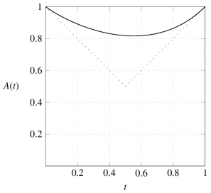
(a) Default asymmetry

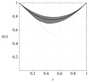
(b) Asymmetry bias correction

Fig. 2: On the left, PF $A(t)=1-t+\exp\{\mathcal{W}_{-1}(-2t/e^{2})+2\}$ arising from the Williamson family (20) for $\theta=1$. Here, $\mathcal{W}_{-1}$ denotes the $k=-1$ branch of the complex Lambert W function. On the right, random PFs built as perturbations around centre (26). All $\theta_{i}$ were sampled from a normal distribution with zero mean and $\sigma=0.1$. We randomly drew a total of 1,000 PFs. The solid line represents the mean function, while the grey envelope represents the confidence interval between quantiles 1% and 99%. The mean line is close to the $A(t)=t^{2}-t+1$ in Fig. 1(a).

2.1.4 Compositional splines

[40] in [40] formalize the construction of a compliant ZBS as a linear combination of the usual B-splines. We shall approximate the CLR space with the ZBS subspace. We refer the reader to [40] for further details on how to compute ZBSs and [6] for more profound knowledge on B-splines, in general.

Splines are bounded functions. Committing to them, we would definitely have $W^{\prime}(0^{+})=-\infty$ and thus $\mathcal{H}_{0}=0$ in (14). Therefore, the resulting spectral measure would be absolutely continuous with respect to the Lebesgue measure on $[0,1]$ with Radon-Nikodym derivative equal to (13).

Given $0=\kappa_{0}<\dots<\kappa_{n+1}=1$, where $n\geq 0$, and assuming $2d$ additional coincidental knots $\kappa_{-d}=\dots=\kappa_{-1}=0$ and $\kappa_{n+2}=\dots=\kappa_{n+d+1}=1$ at the endpoints, the space of splines $p\in\mathcal{Z}_{\bm{\kappa}}^{d}$ of degree less than or equal to $d$ and $n+2$ different knots $\bm{\kappa}=(\kappa_{i})_{i=0}^{n+1}$ has dimension $n+d$. The case $n=0$ corresponds to zero-integral polynomials over $[0,1]$. Altogether, any ZBS can be expressed as

$$p_{\bm{\theta}}(x)=\sum_{i=1}^{n+d}\theta_{i}Z_{i}(x)\,,\ \text{for}\ \bm{\theta}=(\theta_{1},\dots,\theta_{n+d})\in\mathbb{R}^{n+d}\,,$$ (25)

where $\int_{0}^{1}Z_{i}=0$ and we can further assume an orthonormal basis [40], i.e., $\langle Z_{i},Z_{j}\rangle_{L^{2}}=\delta_{ij}$.

Furthermore, we can place a convenient centre for our ZBS space to correct the asymmetry bias. We propose to take $\omega$ in (24) to be the orthogonal projection $z$ of $-(1+\log x)/2$, the case $\theta=2$ in ex:clr-uniform-densities, onto the space (25):

$$z(x)=\sum_{i=1}^{n+d}\left\langle\text{clr}[U^{2}],Z_{i}\right\rangle_{L^{2}}Z_{i}(x)\,.$$ (26)

Fig. 3(a) shows that a spline can effectively approximate the logarithmic centre, despite the divergence near zero. Fig. 3(b) depicts the underlying orthonormal ZBS basis $\{Z_{i}\}$. Fig. 2(b) shows the effectiveness of the bias correction.

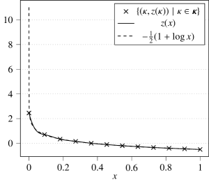
(a) Orthogonal projection

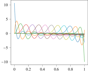
(b) The underlying ZBS

Fig. 3: On the left, the projection $z(x)$ of $-(1+\log x)/2$ onto an orthonormal ZBS 13-dimensional basis with knots $\bm{\kappa}$. The logarithmic function diverges to infinity at zero. On the right, we have the underlying orthonormal cubic ZBS basis with 13 elements.

2.2 Properties

The following sections provide some insights on the relation between the core pdf and the resulting EVC.

2.2.1 Convergence

We will present some results on how convergence on the Bayes space relates to convergence for the resulting EVCs through SBEVC. We shall use the supremum norm $\lVert f\rVert_{\infty}=\sup_{x\in\mathcal{X}}\ \lvert f(x)\rvert$ of a bounded function $f:\mathcal{X}\rightarrow\mathbb{R}$ to measure distances between some objects. $\mathcal{X}$ will typically be a compact subset of $\mathbb{R}^{n}$, namely $[0,1]$, for functions $W$ and $A$, and $[0,1]^{2}$, for copulas $C$. The supremum norm defines a distance $d_{\infty}(f,g)=\lVert f-g\rVert_{\infty}$. A sequence of functions $\{f_{n}\}_{n=1}^{\infty}$ converging on the latter distance to some $f$ is said to converge uniformly. Sometimes, however, uniform convergence is a too strong property. For instance, the function $f$ may not be bounded on the whole $\mathcal{X}$. Another convergence exists in those cases, only requiring the sequence converging uniformly to $f$ on every compact subset $\mathcal{K}\subset\mathcal{X}$. Then, the sequence of $\{f_{n}\}_{n=1}^{\infty}$ is said to be compactly convergent to $f$. The following related concept applies to probability measures.

Definition 2.

def:total-variation Let $\mathbb{P}$ and $\mathbb{Q}$ be probability measures on the space $[0,1]$ equipped with the Borel $\sigma$-algebra $\mathcal{B}$. The total variation distance (TVD) between $\mathbb{P}$ and $\mathbb{Q}$ is defined as

$$d_{\text{TV}}(\mathbb{P},\mathbb{Q})=\sup_{B\in\mathcal{B}}\ \lvert\mathbb{P}(B)-\mathbb{Q}(B)\rvert\,.$$

TVD satisfies all three axioms of a proper metric. By Scheffé’s theorem [54], it can also be expressed in terms of the pdfs $f$ and $g$ of $\mathbb{P}$ and $\mathbb{Q}$, respectively, as

$$d_{\text{TV}}(\mathbb{P},\mathbb{Q})\equiv d_{\text{TV}}(f,g)=\frac{1}{2}\int_{0}^{1}\lvert f(x)-g(x)\rvert\ dx\,.$$ (27)

Our first result links convergence in TVD of a sequence of pdfs with convergence of the corresponding sequence of WTs and their derivatives.

Proposition 2.

prop:fn-converge-imply-wn-converge Let $\{f_{n}\}_{n=1}^{\infty}$ be a sequence of pdfs supported on $[0,1]$ such that $\lim\limits_{n\rightarrow\infty}d_{TV}(f,f_{n})=0$ for some pdf $f$ also on $[0,1]$. Let $W_{n}$ and $W$ be the corresponding Williamson transforms of $f_{n}$ and $f$, respectively. Then, the sequence $\{W_{n}\}_{n=1}^{\infty}$ uniformly converges to $W$ on $[0,1]$. Moreover, $\{W_{n}^{\prime}\}_{n=1}^{\infty}$ compactly converges to $W^{\prime}$ on $(0,1]$.

The next step links the uniform convergence of WTs with that of PFs. Uniform convergence of pointwise-convergent sequences of PFs can be established by other means [20]. Nonetheless, the following result also states the uniform convergence of the first derivatives of PFs under the same hypotheses, which cannot be taken for granted.

Proposition 3.

prop:graph-convergence Let $\{W_{n}\}_{n=1}^{\infty}$ be a sequence of WTs, arising from pdfs, uniformly convergent to some other WT $W$ on $[0,1]$. Also, suppose the sequence of first derivatives $\{W_{n}^{\prime}\}_{n=1}^{\infty}$ of the previous functions compactly converge to $W^{\prime}$ on $(0,1]$. Let $A_{n}$ and $A$ be the corresponding PFs of $W_{n}$ and $W$, respectively, according to SBEVC. Then, the sequence $\{A_{n}\}_{n=1}^{\infty}$ uniformly converges to $A$ on $[0,1]$, while $\{A_{n}^{\prime}\}_{n=1}^{\infty}$ compactly converges to $A^{\prime}$ on $(0,1]$.

Remark 2.

Uniform convergence of function derivatives is mainly unconnected to uniform convergence of the functions themselves. The reason why it works, in this case, comes down to Williamson’s transform, whose first derivative is also in a convenient integral form that allows applying TVD convergence of the internal pdfs to both the function and its derivative simultaneously.

Some topological arguments allow establishing uniform convergence of copulas from pointwise convergence alone [48]. Notwithstanding, there exists a connection between the supremum norms of copulas and those of their respective PFs [37]. Namely, $\lVert C_{1}-C_{2}\rVert_{\infty}\leq 2\gamma/(1+2\gamma)^{1+1/(2\gamma)}$, where $\gamma=\lVert A_{1}-A_{2}\rVert_{\infty}$.

We turn next to some assumptions making convergence in $L_{0}^{2}([0,1])$ sufficient for pdfs to converge in TVD.

Proposition 4.

prop:convergence-tvd-pdfs Let $\{p_{n}\}_{n=1}^{\infty}\subset L_{0}^{2}([0,1])$ continuous and uniformly bounded, i.e., $\lVert p_{n}\rVert_{\infty}\leq K$ for some $K>0$ and for all $n$. Suppose $\lim\limits_{n\rightarrow\infty}\lVert p-p_{n}\rVert_{2}=0$, for some $p\in L_{0}^{2}([0,1])$. Let $f_{n}=\mathrm{clr}^{-1}[p_{n}]$ and $f=\mathrm{clr}^{-1}[p]$. Then, $\lim\limits_{n\rightarrow\infty}d_{TV}(f,f_{n})=0$.

SBEVC, acting on convergent sequences in $L_{0}^{2}([0,1])$, produces EVCs that not only uniformly converge but also whose partial derivatives do. Since copula partial derivatives correspond to conditional CDFs, they are paramount in copula sampling algorithms [7]. cor:convergence-partial-derivatives guarantees that the resulting samples tend to fit the copula uniformly over the support.

Corollary 2.

cor:convergence-partial-derivatives Let $\{z_{n}\}_{n=1}^{\infty}\subset L_{0}^{2}([0,1])$ be a sequence of uniformly bounded smooth cubic ZBSs that converge in the $\lVert\cdot\rVert_{2}$ norm. The corresponding EVCs from SBEVC $\{C_{n}\}_{n=1}^{\infty}$ uniformly converge to some EVC $C$, satisfying $\partial_{i}C_{n}\xrightarrow[n\rightarrow\infty]{\lVert\cdot\rVert_{\infty}}\partial_{i}C$ compactly over $(0,1]^{2}$, for $i=1,2$.

2.2.2 Dependence

In the case of an EVC, Kendall’s tau and Spearman’s rho take the form of integrals involving the PF [37]. The substitution of the PF by the equivalent WT form and a change of variables afterwards do not provide any meaningful insight into the latter’s role. However, the apparent relation between WTs and Lorenz curves reveals a new path for measuring association.

The WT $W$ of a PF $A$ satisfies the definition of a Lorenz [21] curve $L$ after the change of variable $L(x)=W(1-x)$, for $x\in[0,1]$. Lorenz curves appear in econometrics for assessing wealth inequality through the Gini coefficient (GC) $G=1-2\int_{0}^{1}L$. The $G$ index has a geometrical interpretation as the area between $L$ and $x\mapsto x$ divided by the area under $x\mapsto x$, which is equal to $1/2$. The same interpretation applies to $W$ and, since $\int_{0}^{1}W=\int_{0}^{1}L$, we have $G=1-2\int_{0}^{1}W$. A value of $G=0$ means wealth is uniformly distributed (the $p\%$ wealthiest proportion of the population accumulate $p\%$ of the total wealth, for all $p\in[0,1]$), whereas $G\lesssim 1$ means that nearly all wealth belongs to a tiny fraction of the population. In summary, $G=0$ represents perfect equality, while $G=1$ represents perfect inequality.

In our context, a PF $A$ is the affine transformation of some $W$. Since affine transformations change areas by applying a constant factor, the latter cancels out in ratio measures, leaving them invariant. Therefore, the GC is the area between $A$ and the upper bound line $\{y=1\}$ divided by the area between the support lines and the upper bound line. This argument leads to $G=4\left(1-\int_{0}^{1}A\right)$. The value $G=1$ happens when $A$ is identically equal to the lower support lines ($\int_{0}^{1}A=3/4$), producing the comonotonic copula. On the other hand, $G=0$ occurs when $A$ is identical to the upper bound line ($\int_{0}^{1}A=1$), producing the independence copula. This way, the bivariate positive association can be interpreted in econometric terms: comonotonicity is equivalent to perfect inequality, whereas independence corresponds to perfect equality.

The GC is an uncommon association measure in the context of EVCs, despite its simplicity. We have only found a brief mention of it in [31], where the measure was not scaled to lie on $[0,1]$. Moreover, PF symmetry was further assumed. The index can be reformulated for any positively quadrant dependent copula $C$, i.e., $C(u,v)\geq uv$, for all $u,v\in[0,1]^{2}$, as

$$G=4\left(1-\int_{[0,1]^{2}}\frac{\log C(u,v)}{\log uv}\ dudv\right)\,.$$

The GC, as defined above, satisfies the axioms of a dependence measure [7]. The GC takes values on $[0,1]$, unlike Kendall’s tau and Spearman’s rho, which belong to a more general family of concordance measures, ranging in $[-1,1]$ and allowing for negative association.

Remark 3.

Interestingly, after integrating by parts twice, the area of $W$ can be expressed in terms of the inner pdf $f$, yielding $G=1-\mathbb{E}[X],\ \text{where}\ X\sim f$. This means that every GC in $(0,1)$ is attainable through SBEVC.

2.3 Estimation

The estimation process builds upon the various constructions explored above. Given an orthonormal ZBS basis, we aim to find the parameter vector $\bm{\theta}$ that best fits a dataset. Knowing the one-to-one relation [9] between the random vector $(U,V)$ following an EVC and the rv $Z=\log U/\log(UV)$, we reduce our problem to fitting the latter, which has a more straightforward pdf, derived from (2):

$$h(z)=1+(1-2z)\frac{A^{\prime}(z)}{A(z)}+z(1-z)\left[\frac{A^{\prime\prime}(z)}{A(z)}-\left(\frac{A^{\prime}(z)}{A(z)}\right)^{2}\right]\,.$$ (28)

Given a random sample $\mathcal{D}=\{z_{i}\}_{i=1}^{m}$ from $Z$ and a model $h_{\bm{\theta}}$ derived from $p_{\bm{\theta}}$ up to $A_{\bm{\theta}}$, the frequentist approach to the estimation addresses the maximization of the penalized log-likelihood (PLL) of $h_{\bm{\theta}}$

$$\ell(\bm{\theta}|\mathcal{D})=\sum_{i=1}^{m}\log h_{\bm{\theta}}(z_{i})-\lambda\int_{0}^{1}(p_{\bm{\theta}}^{\prime\prime}(x))^{2}\ dx\,\ ,$$ (29)

for some regularization hyper-parameter $\lambda\geq 0$. The square norm term involving $p_{\bm{\theta}}^{\prime\prime}$ is the linearized curvature of the spline: a simplified non-intrinsic form of the curvature that can be expressed as a covariant tensor ${\bm{\theta}}^{\top}\Omega\bm{\theta}$, where $\Omega=(\Omega_{ij})=(\int_{0}^{1}Z_{i}^{\prime\prime}Z_{j}^{\prime\prime})$. Splines may exhibit complex shapes prone to overfitting, as shown in Fig. (3(b)). Penalizing the curvature is the proposed method in [40] in the context of compositional data regression. [32] applied this approach in semiparametric copula models before [32]. Taking $\lambda=0$ removes regularization, retrieving the usual log-likelihood.

Estimating the parameters of such a model poses some challenges. Evaluating the resulting PF from a parameter vector and a single argument implies several non-trivial operations, most notably the integral and affine transformations (16) and (7). These steps can be applied with near-perfect accuracy, with proper algorithms and without time constraints. However, in an iterative optimization, time is scarce. Therefore, we propose critical approximations at each step that trade some accuracy off for processing speed without compromising the overall stability. The effectiveness of our proposal will be thoroughly tested in a SS in Section 3.

First, note that the evaluation of $A$ in (7) at a specific value $t_{0}$ requires solving for $x$ in $t(x)=t_{0}$. The latter will generally be a nonlinear equation that can only be solved through numerical methods at a relatively high computational cost. Hence, in most cases, evaluating (28) in (29) at each point $z_{i}$ becomes rapidly unaffordable as $m$ increases. Moreover, any root finding procedure would prevent us from applying gradient optimization, stopping backpropagation. We propose $h_{\bm{\theta}}$ be approximated by a piecewise linear interpolator $\tilde{h}$ with sufficiently numerous and carefully selected knots.

Since (29) is based on an empirical univariate sample $\mathcal{D}$, a good knot selection utilizes uniform quantiles of $\mathcal{D}$. This way, the knots will be more spaced on low probability regions and accumulate on high probability ones. This criterion, which was employed in a similar setting in [32], reduces the variance of the parameter vector $\bm{\theta}$. Once fixed the quantiles $\{q_{i}\}_{i=1}^{k}$, we need to estimate some $\{x_{i}\}_{i=1}^{k}$ such that $t_{i}\equiv t_{\bm{\theta}}(x_{i})\approx q_{i}$ and then take $h_{i}=h_{\bm{\theta}}(t_{i})$ as the linear interpolator value at knot $t_{i}$. Note that the $t_{i}$’s are approximations for the $q_{i}$’s. To estimate the required $x_{i}$’s, we may apply (8) over the $q_{i}$’s grid using an empirical nonparametric estimate of the PF, like (3). We can state the procedure as follows.

Algorithm 1 (Selection of an interpolation grid for $h_{\bm{\theta}}$).

alg:empirical-w-grid Let $\mathcal{D}=\{z_{i}\}_{i=1}^{m}$ be a random sample following the $H$ distribution. To build an interpolation grid $\{x_{i}\}_{i=0}^{k+1}$ in the $W$ space such that $\{t(x_{i})\}_{i=0}^{k+1}$ are roughly distributed according to $\mathcal{D}$, follow these steps:

1. Pick $k$ uniform quantiles $0=q_{0}<\dots<q_{k+1}=1$ of $\mathcal{D}$.

2. Build the empirical CDF $\tilde{H}$ of $\mathcal{D}$.

3. Build an empirical estimate $\tilde{A}$ using $\tilde{H}$ and (3).

4. Ensure boundary constraints taking

   $$\hat{A}(t)=\min\{1,\max\{t,1-t,\tilde{A}(t)\}\}\,.$$

5. Set $x_{0}=0$ and $x_{k+1}=1$. Then, for every $i\in\{1,\dots,k\}$, set $x_{i}=q_{i}+\hat{A}(q_{i})-1$.

6. Sort ascendingly the resulting $\{x_{i}\}_{i=0}^{k+1}$ and remove duplicates if needed.

We can reuse the grid obtained in the last algorithm throughout the estimation process, at every gradient descent step and with different values for the parameter vector $\bm{\theta}$. With this grid and a parameter vector $\bm{\theta}$, we can now build a light version of $h_{\bm{\theta}}$ to evaluate the PLL. Early experiments suggest that selecting spline knots for $p_{\bm{\theta}}$ according to alg:empirical-w-grid is key to constructing an unbiased estimator $A_{\bm{\theta}}$.

Along with the interpolation grid, we need to estimate the values of $W_{\bm{\theta}}$ and its derivatives from $p_{\bm{\theta}}$.

Algorithm 2 (Approximation of the WT and its derivatives).

alg:estimate-W Let $p_{\bm{\theta}}$ be the ZBS corresponding to the parameter vector $\bm{\theta}$. Let $\{r_{i}\}_{i=0}^{n+1}$ be an strictly increasing real sequence such that $r_{0}=0$ and $r_{n+1}=1$. Let $\epsilon\gtrsim 0$ such that $\epsilon<r_{1}$. To build an approximation to the corresponding WT $W_{\bm{\theta}}$ and its first and second derivatives, follow these steps:

1. For $i\in\{0,\dots,n+1\}$, set $p_{i}=\exp p_{\bm{\theta}}(r_{i})$.

2. Compute $I\approx\int_{0}^{1}\exp p_{\bm{\theta}}$ using the composite trapezoidal rule over $\{(r_{i},p_{i})\}_{i=0}^{n+1}$.

3. For $i\in\{0,\dots,n+1\}$, set $f_{i}=p_{i}/I$.

4. Set $s_{0}=\epsilon$. Then, for $i\in\{1,\dots,n+1\}$, set $s_{i}=r_{i}$.

5. For $i\in\{0,\dots,n+1\}$, set $\bar{W}_{i}^{\prime\prime}=f_{i}/s_{i}$.

6. For $i\in\{0,\dots,n\}$, set $\Delta_{i}=s_{i+1}-s_{i}$.

7. For $i\in\{0,\dots,n\}$, set $P_{i}=\Delta_{i}\ (f_{i}+f_{i+1})/2$ and $Q_{i}=\Delta_{i}\ (\bar{W}_{i}^{\prime\prime}+\bar{W}_{i+1}^{\prime\prime})/2$.

8. Set $\bar{W}_{n+1}^{\prime}=0$. Then, for $i$ from $n$ down to $0$, compute $\bar{W}_{i}^{\prime}$ using the recurrence relation

   $$\bar{W}_{i}^{\prime}=\bar{W}_{i+1}^{\prime}-Q_{i}\,.$$ (30)

9. For $i\in\{0,\dots,n+1\}$, set $\delta_{i}=s_{i}\bar{W}_{i}^{\prime}$.

10. Set $\bar{W}_{n+1}=0$. Then, for $i$ from $n$ down to $0$, compute $\bar{W}_{i}$ using the recurrence relation

    $$\bar{W}_{i}=\bar{W}_{i+1}+\delta_{i}-\delta_{i+1}+P_{i}\,.$$ (31)

11. For $i\in\{0,\dots,n+1\}$, set $W_{i}=\bar{W}_{i}/\bar{W}_{0}$, $W_{i}^{\prime}=\bar{W}_{i}^{\prime}/\bar{W}_{0}$, $W_{i}^{\prime\prime}=\bar{W}_{i}^{\prime\prime}/\bar{W}_{0}$.

12. Build a piecewise linear interpolator $\widetilde{W}^{0}$ from $\{(r_{i},W_{i})\}_{i=0}^{n+1}$ for $W_{\bm{\theta}}$.

13. Build a piecewise linear interpolator $\widetilde{W}^{1}$ from $\{(r_{i},W_{i}^{\prime})\}_{i=0}^{n+1}$ for $W_{\bm{\theta}}^{\prime}$.

14. Build a piecewise linear interpolator $\widetilde{W}^{2}$ from $\{(r_{i},W_{i}^{\prime\prime})\}_{i=0}^{n+1}$ for $W_{\bm{\theta}}^{\prime\prime}$.

Now, we are ready to build a light version of $h_{\bm{\theta}}$.

Algorithm 3 (Approximation of $h_{\bm{\theta}}$ from WT estimates).

alg:h-from-a Let $\{x_{i}\}_{i=0}^{k+1}$ be the interpolation grid from alg:empirical-w-grid. Let $\widetilde{W}^{0}$, $\widetilde{W}^{1}$ and $\widetilde{W}^{2}$ be the piecewise linear approximations to $W_{\bm{\theta}}$, $W_{\bm{\theta}}^{\prime}$ and $W_{\bm{\theta}}^{\prime\prime}$ from alg:estimate-W, respectively. To build an approximation for $h_{\bm{\theta}}$, follow these steps:

1. For $i\in\{1,\dots,k\}$, set $W_{i}=\widetilde{W}^{0}(x_{i})$, $W_{i}^{\prime}=\widetilde{W}^{1}(x_{i})$, $W_{i}^{\prime\prime}=\widetilde{W}^{2}(x_{i})$.

2. Set $t_{0}=0$ and $t_{k+1}=1$. Then, for $i\in\{1,\dots,k\}$, set $t_{i}=(1+x_{i}-W_{i})/2$.

3. For $i\in\{1,\dots,k\}$, set $A_{i}=(1+x_{i}+W_{i})/2$.

4. For $i\in\{1,\dots,k\}$, set $M_{i}=1-W_{i}^{\prime}$.

5. For $i\in\{1,\dots,k\}$, set $A_{i}^{\prime}=(1+W_{i}^{\prime})/M_{i}$.

6. For $i\in\{1,\dots,k\}$, set $A_{i}^{\prime\prime}=4W_{i}^{\prime\prime}/M_{i}^{3}$.

7. For $i\in\{1,\dots,k\}$, set $D_{i}=A_{i}^{\prime}/A_{i}$.

8. Set $h_{0}=h_{k+1}=0$. Then, for $i\in\{1,\dots,k\}$, set

   $$h_{i}=1+(1-2t_{i})D_{i}+t_{i}(1-t_{i})\left(\frac{A_{i}^{\prime\prime}}{A_{i}}-D_{i}^{2}\right)\,.$$ (32)

9. Build a piecewise linear interpolator $\tilde{h}$ from $\{(t_{i},h_{i})\}_{i=0}^{k+1}$.

10. Compute $I\approx\int_{0}^{1}\tilde{h}$ using the composite trapezoidal rule over $\{(t_{i},h_{i})\}_{i=0}^{k+1}$.

11. Use $\hat{h}=\tilde{h}/I$ as an approximation for $h_{\theta}$ over $[0,1]$.

alg:h-from-a deals with problems like the approximation of $h_{\bm{\theta}}$ and the rotation of $W_{\bm{\theta}}$. On the other hand, alg:estimate-W formalizes an efficient computation scheme for $W_{\bm{\theta}}$. Both together allow computing $\ell(\bm{\theta}|\mathcal{D})$. Fig. 4 shows the full computation graph. Gradients flow from the top PLL down the parameter vector using backpropagation. We recommend using the autograd package [41], capable of performing automatic differentiation on native Python operations. Some representative routines in our implementation are numpy’s trapz, for calculating integrals using the trapezoidal rule, and cumsum, for computing recurrences (30) and (31).

Fig. 4: Computation graph for the estimation process, from the bottom parameter vector $\bm{\theta}$ up to the PLL $\ell(\bm{\theta}|\mathcal{D})$.

Implementation tips

alg:estimate-W and alg:h-from-a use discretization to approximate functions and integrals. The finer-grained the discretization steps, the lower the error and the higher the computation time. A trade-off between those dimensions is needed. On the other hand, knowing $W_{\bm{\theta}}^{\prime}(0^{+})=-\infty$ and $W_{\bm{\theta}}^{\prime\prime}(0^{+})=\infty$, we recommend choosing the grid in alg:estimate-W so that points accumulate near zero, making the linear interpolation more effective. Chebyshev nodes are a standard option.

To facilitate SBEVC’s estimation process, we propose to change the copula variable ordering whenever a steep slope is likely to appear for $W_{\bm{\theta}}$ near zero, which coincides with the minimum of $A_{\bm{\theta}}$ being placed at $t<0.5$. We can heuristically assess this situation by calculating the mode of the pdf $h$, as suggested in [19]. If the mode appears at $t<0.5$, the PF’s minimum will likely be placed at $t<0.5$. We support the hypothesis of [19] based on our own experience. Therefore, whenever the mode peaks at $t<0.5$, we recommend changing the variable ordering before estimating and then flipping the resulting PF $A$ as $\tilde{A}(t)=A(1-t)$.

2.4 Simulation

Once the parameters $\bm{\theta}$ have been estimated, we propose to build $W_{\bm{\theta}}$ and $A_{\bm{\theta}}$ subsequently. From that point on, querying the model (simulating, estimating probabilities, among others) will be equivalent to evaluating the PF $A_{\bm{\theta}}$, as with any other EVC.

The algorithms in Section 2.3 stand valid, with some minor and convenient changes. Since we only need to build the functions once, and not once per iteration, we may employ more expensive and accurate approximations. In particular, $W_{\bm{\theta}}^{\prime\prime}$ can be evaluated without approximations. More sophisticated procedures should replace trapezoidal rules and linear interpolations. On the other hand, alg:empirical-w-grid is no longer required. Instead, we may employ a root-finding algorithm to invert the automorphism $t$.

The interpolation points of $A_{\bm{\theta}}$ could be input to the shape-preserving interpolation procedure by [49], which would guarantee that the resulting spline is convex over the whole domain [49]. However, in general, the second derivative of such a spline would not be continuous, which would hinder the simulation process. In practice, we recommend smoothness and accuracy over shape preservation, provided a sufficiently fine interpolation grid is used.

Finally, to draw samples from $C_{\bm{\theta}}$, we recommend the general algorithm in [7], which only requires inverting one of its partial derivatives [16, 19]. The root-finding algorithm in [3] proves to be highly effective.

2.5 Refinement

One of the limitations of SBEVC is the fact that an estimated PF $A$ always satisfies $A^{\prime}(0^{+})=-1$ and $A^{\prime}(1^{-})=1$. These constraints are a consequence of our construction, which imposes $W^{\prime}(0^{+})=-\infty$ and $W^{\prime}(1^{-})=0$ on the WT. In practice, however, these boundary constraints do not hinder the expressiveness of the resulting model. Remember that, for instance, upper tail dependence does not relate to either boundary derivative of the PF, but the mid-point value $A(1/2)$. This fact contrasts with the nature of another semiparametric procedure like [32], where a slope value entirely determined the tail index.

In SBEVC, misspecified slopes for the PF have a much lower impact on the concordance (Blomqvist’s beta) and upper tail dependence. Nonetheless, since it might produce a slight bias, we propose a refinement step that could complement SBEVC.

[38]’s method is best known for inducing asymmetry in symmetrical EVCs [38]. However, there is no reason why it could not apply to asymmetrical ones [47]. Consider a PF $A$ obtained through SBEVC. Differentiating (1), we arrive at

$$\begin{array}[]{r@{\ }c@{\ }l}A_{\alpha,\beta}^{\prime}(0^{+})&=\beta A^{\prime}(0^{+})&=-\beta\\ A_{\alpha,\beta}^{\prime}(1^{-})&=\alpha A^{\prime}(1^{-})&=\alpha\end{array}\,,$$ (33)

where, remember, $\alpha,\beta\in(0,1]$, retrieving $A$ for $\alpha=\beta=1$. Even though $A$ is, in general, asymmetrical, we see from (33) that [38]’s method serves our purpose of freely parameterizing the boundary slopes.

We believe that adding two more parameters through [38]’s method may improve the fitness of the resulting model in some particular cases, especially for weak correlations. However, the inclusion of the new parameters in the gradient-based optimization seems unworkable, as it would invalidate the interpolation grid in alg:h-from-a. A derivative-free optimization involving both the spline parameter vector $\bm{\theta}$ and the asymmetry parameters $\alpha$ and $\beta$ could be run, starting from $\alpha=\beta=1$ and some initial guess $\bm{\theta}=\bm{\theta}_{0}$ obtained through a gradient-based method.

3 Results

We will test SBEVC on simulated and actual data. In both scenarios, we will compare SBEVC with the methodology by [13] [13]. We shall refer to their method as constrained B-splines (COBS). We have chosen COBS for its flexibility and simplicity, sharing three relevant traits with SBEVC: complying with PF constraints, using splines and exclusively addressing bivariate EVCs.

3.1 Preliminaries

Before diving into the specific settings of each experiment, let us clarify some shared configuration aspects.

3.1.1 Optimization

We performed all SBEVC estimates using standard Python scientific packages like numpy and scipy, and automatic differentiation, thanks to autograd [41]. Namely, we employed scipy’s implementation of the L-BFGS-B algorithm by [8] [8]. We assessed convergence by setting the ftol=1e-6 configuration parameter in the minimize routine, which targets the relative change in the loss function between iterations. Even though this value is very conservative, the procedure converges well, with reasonable execution times, as we will see.

All estimation runs started at the null spline, with all coordinates equal to zero, regardless of using a fixed affine centre. Despite the caveats by [32] [32], as demonstrated in [50], current optimization methods can deal with complex problems even if the initial parameter values are far from the optimal solution. Notwithstanding, we agree with [32] that good initial guesses would speed up the process.

COBS is very easy to implement on top of the cobs R package [13]. The R execution environment can be accessed from Python thanks to the rpy2 Python package with little coding overhead. Specifically, we employed the main cobs routine, selecting a smoothing splines regression of degree two by entering lambda=-1. We raised the maximum number of iterations until convergence to 1,000 using the maxiter parameter. We kept the maximum number of spline knots to the default value of 20. Both the knots selection and the smoothing penalty was internally chosen by cobs. The convexity requirement was introduced by setting constraint="convex". The boundary constraints were enforced over a fine 1,001-point equally-spaced grid over $[0,1]$ using the pointwise argument. Finally, we interpolated cobs’ result over the former grid using cubic splines to allow for continuous second derivatives.

3.1.2 Resources

Both the SS and actual data application would not have been possible without the vast repertoire of software artefacts and services currently available.

First, SBEVC, fully implemented in Python, was containerized using [15] [15], which, apart from being ideal for achieving reproducible research, also helped to move our execution environment to the cloud with [52] [52]. [15] was also helpful for preparing a maintainable execution environment with Python and R, as required by cobs.

While developing and testing, we employed a local [53] cluster [53] on an Intel^® Core^© i7-4700MQ CPU laptop with eight 2.40 GHz cores and 15.6 GiB of memory and operating system Ubuntu 20.04.3 LTS. We entrusted the bulky SS final executions to a cloud provider. The Kubernetes service comprised 50 dynamically allocated nodes running on possibly different Intel^® Xeon^© architectures with Ubuntu 18.04. Overall, each node counted on two virtual CPUs and seven GiB of memory at any given time. Due to Kubernetes’ requirements, only one CPU was available for Spark per node.

We sped up the experiments parallelizing specific tasks with [51] [51]. To prepare the [51] setting with [52], two artefacts were of great help: the [14] [14] and the [27] [27].

Finally, [4] [4] turned out to be helpful to manage all our [52] experiments from the same friendly user interface, connecting the [52] cluster to the Git repository.

Supplementary materials

Access to source code and other deliverables will be provided upon acceptance for publication.

3.2 Simulation study

We conducted a SS to test the effectiveness of SBEVC on a broad spectrum of cases with high confidence. The SS consists of three experiments. The first one addresses the bias and variance tradeoffs by repeating the estimation process for many random samples drawn from a fixed copula in Table 1 for several parameter configurations. The second experiment covers an even more extensive array of EVCs while focusing on validation through TVD. Then, the third one compares SBEVC with COBS in terms of the root mean integrated squared error (RMISE) in several scenarios with varying dependence strengths, asymmetries and sample sizes.

SBEVC entails numerous non-trivial analytic and geometric transformations. Even though we could argue that none of them exceeds a reasonable level of complexity, clever algorithms and powerful computational resources are still needed for it to work in practice. In particular, optimization algorithms are vital to finding solutions that maximize (29) under memory and time constraints. The joint behaviour of all these pieces is difficult to assess from a purely theoretical perspective without simulations.

Common settings

Throughout the SS, copula models build upon a cubic orthonormal ZBS basis. The grid size was 200 both in alg:estimate-W and alg:h-from-a ($n+2=200$ and $k+2=200$, respectively). Also, we took $\epsilon=10^{-9}$ in alg:estimate-W. These settings express an adequate balance between approximation accuracy and reasonable execution times.

3.2.1 Bias and variance

The first part of the SS consisted of 30 individual experiments, focusing on a particular instance of a copula family. For each copula instance, we performed an estimation run with SBEVC on each of 100 different random samples from the copula for 3,000 runs. Then, for each 100-sample experiment, we collected the pointwise means and pointwise 98% confidence intervals of the estimated PFs and compared both functional statistics with the original PF. We handled each random sample as an independent [51] task to speed up computations.

We employed the two families in Table 1: the Gumbel and the Galambos families. These are probably two of the most well-known EVCs. [23] even studied and found a relation between the two in [23], knowing the similarity of their PFs. In each copula family, we tested up to five different values of the unique parameter $\theta$, giving rise to different correlation levels. Finally, apart from the pure form of each Gumbel or Galambos copula, we introduced asymmetry through [38]’s device, taking either $\alpha$ or $\beta$ equal to $0.5$ and leaving the other as $1$. This configuration was precisely the one that demonstrated higher asymmetry in [24]. As a side note, we remind that the asymmetrical extensions of the Gumbel and Galambos families are known as the Tawn and Joe families, respectively.

Each of the random copula samples consisted of 1,000 observations. Our models were fit using 13 parameters in all cases: 10 more than the ground truth copula families. We believe that the specific number of parameters has less impact in a semiparametric context, where one typically employs a large number and then reduces overfitting by penalizing curvature. In the end, the target of this semiparametric method is a function that lives in an infinite-dimensional space. In practice, both the Gumbel and the Galambos families need fewer parameters than 13, but in this case, we have preferred to stick to a large number to showcase the method’s performance in a general setting. Finally, for both the Gumbel and Galambos copulas, we used a curvature penalty factor $\lambda=10^{-5}$.

Fig. 5 shows the results for the Gumbel copulas, while Fig. 6 presents those of the Galambos. The results are qualitatively very similar. SBEVC displays low biases and variances in all cases. If any, the highest biases appear under asymmetry and low correlations. This behaviour matches the known limitation of SBEVC as regards the boundary slopes, which have fixed values. Variance is also higher for small correlations, in agreement with [37].

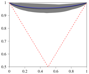
(a) $\theta=1.1$, $\alpha=0.5$, $\beta=1$

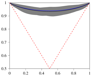
(b) $\theta=1.1$, $\alpha=1$, $\beta=1$

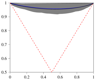
(c) $\theta=1.1$, $\alpha=1$, $\beta=0.5$

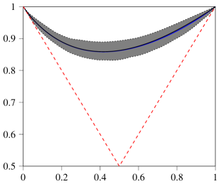
(d) $\theta=1.5$, $\alpha=0.5$, $\beta=1$

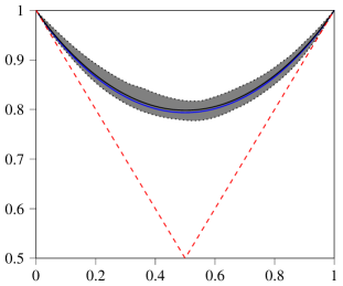
(e) $\theta=1.5$, $\alpha=1$, $\beta=1$

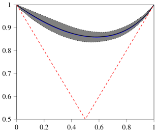
(f) $\theta=1.5$, $\alpha=1$, $\beta=0.5$

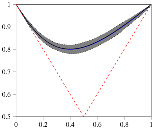
(g) $\theta=2$, $\alpha=0.5$, $\beta=1$

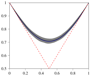
(h) $\theta=2$, $\alpha=1$, $\beta=1$

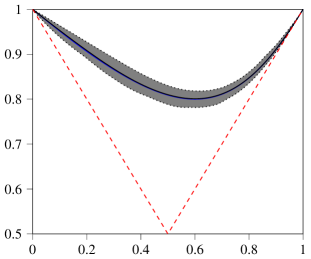
(i) $\theta=2$, $\alpha=1$, $\beta=0.5$

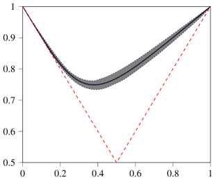
(j) $\theta=3$, $\alpha=0.5$, $\beta=1$

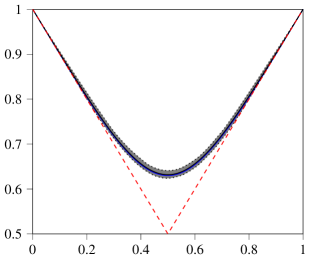
(k) $\theta=3$, $\alpha=1$, $\beta=1$

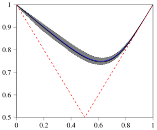
(l) $\theta=3$, $\alpha=1$, $\beta=0.5$

(m) $\theta=4$, $\alpha=0.5$, $\beta=1$

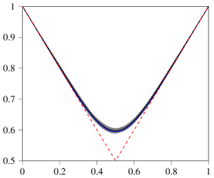
(n) $\theta=4$, $\alpha=1$, $\beta=1$

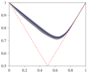
(o) $\theta=4$, $\alpha=1$, $\beta=0.5$

Fig. 5: SS for the Gumbel family. The blue line designates the ground-truth PF, whereas the black corresponds to the estimations’ pointwise mean. The shaded areas represent 98% pointwise confidence intervals for the estimates.

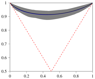
(a) $\theta=0.5$, $\alpha=0.5$, $\beta=1$

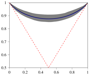
(b) $\theta=0.5$, $\alpha=1$, $\beta=1$

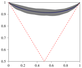
(c) $\theta=0.5$, $\alpha=1$, $\beta=0.5$

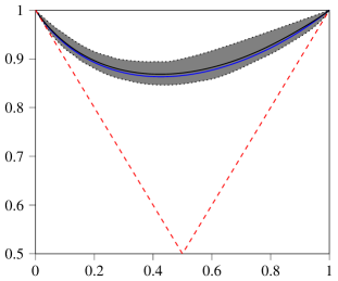
(d) $\theta=0.75$, $\alpha=0.5$, $\beta=1$

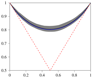
(e) $\theta=0.75$, $\alpha=1$, $\beta=1$

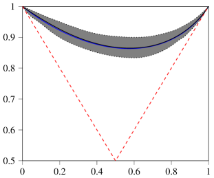
(f) $\theta=0.75$, $\alpha=1$, $\beta=0.5$

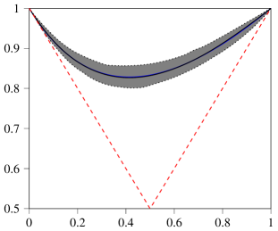
(g) $\theta=1$, $\alpha=0.5$, $\beta=1$

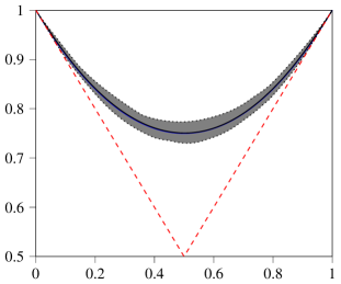
(h) $\theta=1$, $\alpha=1$, $\beta=1$

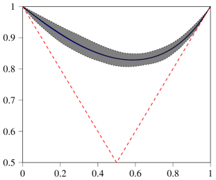
(i) $\theta=1$, $\alpha=1$, $\beta=0.5$

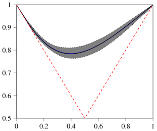
(j) $\theta=1.5$, $\alpha=0.5$, $\beta=1$

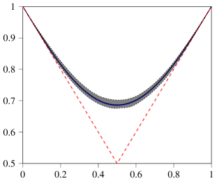
(k) $\theta=1.5$, $\alpha=1$, $\beta=1$

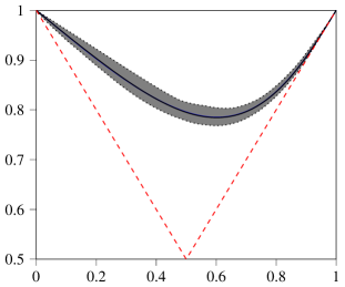
(l) $\theta=1.5$, $\alpha=1$, $\beta=0.5$

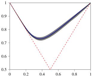
(m) $\theta=3$, $\alpha=0.5$, $\beta=1$

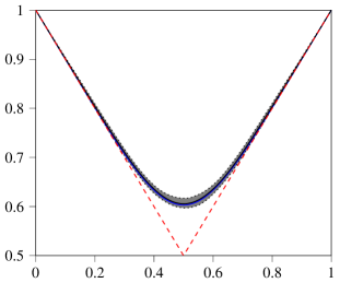
(n) $\theta=3$, $\alpha=1$, $\beta=1$

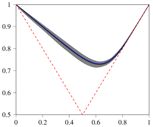
(o) $\theta=3$, $\alpha=1$, $\beta=0.5$

Fig. 6: SS for the Galambos family. The blue line designates the ground-truth PF, whereas the black corresponds to the estimations’ pointwise mean. The shaded areas represent 98% pointwise confidence intervals for the estimates.

In all simulations, we employed the trick mentioned in Section 2.3 for selecting the a priori more convenient variable ordering to avoid numerical instabilities. The procedure worked well, as demonstrated by the nearly identical results obtained for either $\alpha=0.5$ or $\beta=0.5$.

Execution details

We approximately recorded the execution times for the 30 experiments with the assistance of the Spark Web UI. Roughly 50% finished in three minutes, 75% in four and 90% in seven. Consistently below eight minutes, the most time-consuming experiments correspond to the highest correlated Gumbel and Galambos copulas. That is presumably because the optimal solution was furthest from the starting null vector. Since there were 100 tasks on each job and the cluster only had 50 nodes, we could expect the average execution time to be half of the previous values.

3.2.2 Total variation

In the second part of the SS, we generated $n=200$ random SBEVCs. We chose the affine spline model with centre (26) as the first building block, assuming uniformly distributed knots and $d=13$ parameters. Let us call $\bm{\theta}_{0}\in\mathbb{R}^{d}$ the coordinates of the centre of the affine model. We then ran an MCMC simulation assuming the model coordinates $\bm{\theta}$ in (24) were distributed according to the following pdf:

$$p({\bm{\theta}})\propto\left\{\begin{aligned} e^{-\lambda{\bar{\bm{\theta}}}^{\top}\Omega\bar{\bm{\theta}}}\,,&\ \text{if}\ \lVert\bm{\theta}\rVert_{2}\leq R\\ 0\,,&\ \text{if}\ \lVert\bm{\theta}\rVert_{2}>R\end{aligned}\right.\,,\ \text{for}\ \bar{\bm{\theta}}=\bm{\theta}+\bm{\theta}_{0}\,,$$

where $\Omega$ is the curvature matrix of the underlying spline, as described in Section 2.3, and $\lambda$ and $R$ are tuning parameters. The previous model is the truncated version of an improper prior based on curvature penalization, with factor $\lambda$. The support of the distribution is the hyperball of radius $R$.

We tuned the parameters with values $\lambda=10^{-4}$ and $R=5$ so that the resulting splines covered a wide range of correlations (in the sense of the GC) and were, at the same time, smooth. Finally, to prevent any asymmetry, we replaced the even elements in the sequence with their corresponding mirrored versions $\tilde{A}(t)=A(1-t)$. Fig. 7 shows a subsample of the generated random PFs. They cover the area between the support lines and the upper bound line in a reasonably balanced way. We also employed the heuristic to determine the most suitable variable ordering in this part of the SS. Hence, we expected SBEVC to perform well regardless of the orientation of the PF.

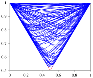
Fig. 7: A subsample of size 100 from the whole population of random PFs used in the second part of the SS.

For each element in the sequence $\{\bm{\theta}_{i}\}_{i=1}^{n}$, we built the EVC $C_{\bm{\theta}_{i}}$ and performed several estimation runs on random samples of different sizes $\{S_{j}\}_{j=1}^{m}$. All fitted models had the same number of parameters as the ground truth splines ($d=13$) and employed the same affine translation. The penalty factor in the loss function (29) was also set to $\lambda=10^{-4}$. The only aspect in which estimated models differed from ground truth is spline knot placement, which was uniform for the latter, but empirically assessed for the former. Then, for each sample size $S_{j}$, we estimated a copula $C_{ij}$ using SBEVC and assessed divergence from ground truth through TVD

$$d_{\text{TV}}(C_{\bm{\theta}_{i}},C_{ij})=\frac{1}{2}\int_{[0,1]^{2}}\lvert c_{\bm{\theta}_{i}}(u,v)-c_{ij}(u,v)\rvert\ dudv\,,$$ (34)

where $c_{\bm{\theta}_{i}}$ and $c_{ij}$ are the pdfs of $C_{\bm{\theta}_{i}}$ and $C_{ij}$, respectively. The TVD defined in (34) is the bivariate counterpart of def:total-variation and thus provides an upper bound on the difference between the measured values of each copula on any measurable set $B\subset[0,1]^{2}$. Therefore, (34) is a very conservative evaluation measure.

Table 2 presents the main summary statistics from the experiment. Each [51] task targeted a different random EVC. Then, each task comprised four estimation runs. The table shows promising results, considering the complexity of the ground truth models and the finiteness of samples. Mean values are typically below $0.05$, whereas the 75% and 90% quantiles do not surpass the $0.10$ threshold. Table 2 shows that TVD decreases as the sample size increases. Fig. 8 reveals some outliers, which become rarer with larger sample sizes. Besides, Fig. 8 suggests SBEVC can handle even the highest correlated samples well. The outliers are due to the sensitivity of the TVD metric to deviations in highly correlated samples. As Fig. 9 shows, the TVD metric positively correlates with the GC even for moderate values of the latter.

	mean	10%	25%	50%	75%	90%
sample size
250	.06642	.0226	.03237	.04578	.06279	.08914
500	.04591	.01562	.02492	.03797	.05527	.07525
1000	.03701	.01333	.0213	.03093	.04301	.05994
2000	.0322	.01157	.01681	.02518	.03421	.05841

Table 2: Main summary statistics from the second part of the SS, mean and quantiles, for each sample size. TVD decreases as sample size increases.

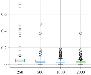
Fig. 8: Box plots of the TVD distributions for each sample size.

Fig. 9: Regression tree (depth 2) of TVD on the GC for sample size 2,000. On average, SBEVC performs well even on the seven instances with GC above 98%.

Execution details

The total execution time for the 200 random EVCs was roughly one hour. Considering the cluster only had 50 nodes, the average execution time for a task in this experiment was approximately 15 minutes.

3.2.3 RMISE

The third part of the SS consisted of 20 individual experiments with different settings. We generated 100 random samples in each experiment and fitted them using SBEVC and COBS. Then, we collected the squared $L^{2}([0,1])$ distances between the ground-truth PF and the estimated PF through SBEVC and COBS. For each estimation method, these measures were averaged to approximate the RMISE like in [55]. The lower the RMISE, the better the technique. We also assessed the statistical significance of the results through a Wilcoxon signed-rank test applied on the unaggregated squared $L^{2}([0,1])$ distances, assuming the null hypothesis that COBS produces better results than SBEVC. As in the previous parts of the SS, we used for SBEVC $d=13$ ZBS elements and the curvature penalty factor was $\lambda=10^{-4}$.

	$\mathrm{RMISE}(\mathrm{SBEVC})$	$\mathrm{RMISE}(\mathrm{COBS})$	p-value
settings
$\theta=1.1$, $\beta=0.5$, $n=250$	.02375	.04314	2.29E-08
$\theta=1.1$, $\beta=0.5$, $n=1000$	.01441	.02611	4.57E-10
$\theta=1.1$, $\beta=1.0$, $n=250$	.02497	.04534	7.80E-07
$\theta=1.1$, $\beta=1.0$, $n=1000$	.01283	.02362	2.60E-10
$\theta=1.5$, $\beta=0.5$, $n=250$	.02097	.04466	1.15E-13
$\theta=1.5$, $\beta=0.5$, $n=1000$	.01198	.02749	9.90E-16
$\theta=1.5$, $\beta=1.0$, $n=250$	.01518	.04018	5.15E-14
$\theta=1.5$, $\beta=1.0$, $n=1000$	.00807	.02326	4.64E-14
$\theta=2.0$, $\beta=0.5$, $n=250$	.01558	.04233	5.86E-15
$\theta=2.0$, $\beta=0.5$, $n=1000$	.00839	.02384	1.14E-15
$\theta=2.0$, $\beta=1.0$, $n=250$	.01116	.02854	1.15E-13
$\theta=2.0$, $\beta=1.0$, $n=1000$	.00527	.01835	6.94E-17
$\theta=3.0$, $\beta=0.5$, $n=250$	.01276	.03909	1.21E-17
$\theta=3.0$, $\beta=0.5$, $n=1000$	.00626	.02494	5.20E-17
$\theta=3.0$, $\beta=1.0$, $n=250$	.00721	.04049	2.82E-14
$\theta=3.0$, $\beta=1.0$, $n=1000$	.00490	.01568	1.34E-15
$\theta=4.0$, $\beta=0.5$, $n=250$	.01128	.03556	7.79E-17
$\theta=4.0$, $\beta=0.5$, $n=1000$	.00487	.02241	5.74E-18
$\theta=4.0$, $\beta=1.0$, $n=250$	.00986	.05981	1.92E-15
$\theta=4.0$, $\beta=1.0$, $n=1000$	.00513	.01135	7.04E-08

Table 3: A comparison between SBEVC and COBS based on RMISE. All settings refer to the parametric Gumbel family in Table 1. RMISE is statistically significantly lower for SBEVC.

The RMISE results are presented in Table 3. Each row corresponds to a different experiment. The left-most column shows the experiment settings. The underlying parametric copula belongs to an asymmetrical Gumbel family (see Table 1) using [38]’s device (1). Then, $\theta$ is the parameter of the Gumbel copula and $\beta$ is one of the asymmetry parameters, fixing $\alpha=1$ as a constant throughout all configurations. The combinations of $\theta$, and $\beta$ are precisely those that appear in the mid and right columns in Fig. 5. We draw samples from each copula configuration with a medium ($n=1,000$) and a small ($n=250$) sample size. As we can see, SBEVC significantly outperforms COBS in all circumstances, roughly halving the RMISE.

3.3 Case study

The following sections will solve a statistical modelling and simulation problem on LIGO and Virgo’s precious gravitational wave (GW) detection data. The aim of this case study is twofold. On the one hand, we will examine the steps in the construction and estimation of SBEVCs with an authentic hands-on experience. On the other hand, we aim to compare SBEVC with COBS on non-synthetic samples. After some sensible transformations, LIGO and Virgo’s data have an EVC dependence structure. The underlying copula presents a very different look than what we have seen in Fig. 5 and Fig. 6.

3.3.1 History

In 2015, the LIGO Scientific Collaboration and the Virgo Collaboration announced the first direct detection of a GW, produced by the merger of a binary black hole [1]. The existence of GWs, ripples in the fabric of space-time, was predicted by Einstein’s theory of general relativity in 1916 as a mathematical construct that many thought to have no physical meaning [10]. It took nearly a century from its prediction and 60 years of search to experimentally ascertain the discovery, opening a new era for astronomy.

Only the most extreme events in the Universe, in terms of energy, can generate GWs strong enough to be detected by current experimental procedures due to the small value of the gravitational constant [10], which expresses the rigidity of space-time. A significant amount of human and material resources are needed to detect GWs. Specifically, sufficiently sensitive interferometers need to have arms several kilometres long. Additionally, in order to discriminate between true detections and spurious local signals (like electromagnetic radiation or earthquakes), several detectors, far apart from each other, are needed.

LIGO, settled in the United States, with two laboratories, was the first detector of an advanced global network that aims to increase discoveries’ accuracy and exhaustiveness [1], soon to be joined by others, most notably Virgo, in Italy. Despite LIGO and Virgo joining efforts, it was LIGO that reported the first detection since the Virgo facilities were not operating at that time for upgrading reasons. Since the first detection in 2015, the collaboration of LIGO and Virgo has confirmed 50 events. They all correspond to massive body mergers, mainly black holes and neutron stars.

3.3.2 Data

We have chosen the GW detection dataset gathered by the LIGO and Virgo collaborations during their first three observation runs to test the applicability of SBEVC. It consists of 50 rows and two columns. Each row represents a merger event, while each column features one of the masses involved in the event, measured in solar mass units (M_$\odot$). During the first and second observation runs, 11 events were detected, while the third run provided 39. The first event was GW150914, in September 2015, and the last one, GW190930_133541, in September 2019. LIGO and Virgo report the larger of the two masses, the primary mass, as the first tuple component, followed by the secondary mass.

We believe that very few datasets better represent bivariate data, considering the very nature of binary mergers. Bivariate models are usually building blocks for higher-dimensional ones, but in this case, all the attention is focused on two mass values of high scientific relevance. Another aspect that adds to this significance is the scarcity of data, for only 50 events have been recorded during five years. This scarcity contrasts with the increasingly large amounts of information coming from IoT, social networks, finance, among others, in the current era of Big Data.

3.3.3 Model

As mentioned above, the dataset consists of 50 bivariate observations $\mathcal{D}=\{(M_{1}^{(i)},M_{2}^{(i)})\}_{i=1}^{50}$, where $M_{1}^{(i)}\geq M_{2}^{(i)}$. The last censoring constraint makes the dataset not directly tractable by usual copulas, supported on the whole $[0,1]^{2}$, unless conveniently preprocessed.

LIGO and Virgo perform a statistical analysis of the joint mass distribution [2]. They consider two separate univariate models. The first one models the primary mass $M_{1}$ unchanged, whereas the second one models the mass ratio $Q=M_{2}/M_{1}$ conditioning on $M_{1}$. Since $M_{1}\geq M_{2}$, by definition, the resulting model captures by construction the censoring constraint. The final joint model is formed by the vector $(M_{1},QM_{1})$.

Instead of considering an auxiliary ratio variable, we directly model a bivariate mass vector. We turned the censoring problem into an exchangeable one, where both masses played the same role. The original dataset $\mathcal{D}$ does not allow such a treatment, so we hypothesized a new sample space where primary masses are detected with 50% probability at the first vector component and 50% at the second one. This scenario corresponds to detections reporting masses without considering their relative order. Therefore, we built a new sample $\widetilde{\mathcal{D}}=\{(\widetilde{M}_{1}^{(i)},\widetilde{M}_{2}^{(i)})\}_{i=1}^{100}$, where $\widetilde{M}_{j}^{(i)}=M_{j}^{(i)}$ or $\widetilde{M}_{j}^{(i)}=M_{1+j\bmod 2}^{(i-50)}$, respectively, if $i\leq 50$ or $i>50$. We then targeted a random vector $(\widetilde{M}_{1},\widetilde{M}_{2})$. To retrieve the original primary-secondary mass model, we just had to take $M_{1}=\max\{\widetilde{M}_{1},\widetilde{M}_{2}\}$ and $M_{2}=\min\{\widetilde{M}_{1},\widetilde{M}_{2}\}$.

Using the previous up-sampled and symmetrical dataset, we fitted (i) a single univariate mass model $f$ for both margins and (ii) a copula model $C$ of the dependency between mass ranks.

Univariate margin model

We decided to employ a semiparametric model for the univariate margin mass model. We successfully tried the same technique we used for modelling the density $f$ in (16): Bayes space pdfs built from ZBSs.

The result of our experiment is shown in Fig. 10. We selected 17 parameters, with knots distributed according to the original sample between 1 M_$\odot$ and 100 M_$\odot$, and a curvature penalty factor of 10. The first mode, near 1 M_$\odot$, mostly corresponds to neutron stars; black hole masses typically range beyond 5 M_$\odot$.

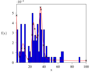
Fig. 10: Univariate margin mass model. The pdf is displayed on the left, whereas the quantile function is on the right. In both cases, the fitted model shows in red and the empirical estimate is in blue. The vertical cuts on the left correspond to the underlying spline knots.

Bivariate copula model

Letting $\hat{F}$ be the empirical CDF of the univariate sample $\{\widetilde{M}_{1}^{(i)}\}_{i=1}^{100}$ (equivalently, from $\{\widetilde{M}_{2}^{(i)}\}_{i=1}^{100}$), we decided to fit a copula pseudo-sample $\widetilde{\mathcal{D}}_{\text{cop}}=\{(\widetilde{U}_{1}^{(i)},\widetilde{U}_{2}^{(i)})\}_{i=1}^{100}=\{(\hat{F}(\widetilde{M}_{1}^{(i)}),\hat{F}(\widetilde{M}_{2}^{(i)}))\}_{i=1}^{100}$ independent of the fitted margin model from the previous section.

The applicability of EVCs was readily made clear after inspecting $\widetilde{\mathcal{D}}_{\text{cop}}$, where the mirrored data points resembled some characteristic patterns we saw during a random EVC generation run à la Fig. 7. Namely, they outlined two curved paths that met at both the lower and upper tail corners.

Data inspection also revealed the absence of upper tail dependence, while lower tail dependence was present. This behaviour did not match the features of EVCs: in practice, they never have lower tail dependence, but they do exhibit dependence in the upper tail. Interestingly, we can resort to survival copulas whenever a switch between lower and upper tails is needed [19]. If a random vector with uniform margins $(U,V)$ is distributed according to a copula $C$, then $(1-U,1-V)$ follows the survival copula [7, 25] $\check{C}(u,v)=u+v-1+C(1-u,1-v)$. The bivariate copula sample $\widetilde{\mathcal{D}}_{\text{cop}}$ was accordingly transformed into $\widetilde{\mathcal{D}}_{\text{surv}}=\{(1-\widetilde{U}_{1}^{(i)},1-\widetilde{U}_{2}^{(i)}))\}_{i=1}^{100}$. Once $\check{C}$ fits $\widetilde{\mathcal{D}}_{\text{surv}}$, the original copula can be retrieved by taking $C$ equal to the survival copula of $\check{C}$.

An extreme-value dependence test [26], implemented in the function evTestK of the R package copula [33, 34, 36, 43], confirmed our intuition about the applicability of EVCs, yielding a p-value higher than 0.35.

The SBEVC model builds upon a cubic (orthonormal) ZBS basis with 13 elements, a curvature penalty factor of $10^{-5}$ and interpolation grid sizes of $k+2=80$, in alg:h-from-a, and $n+2=200$, in alg:estimate-W. The value of the latter setting is lower than the one employed in the SS based on the reduced sample size. On the other hand, we used the same COBS configuration as in Section 3.2.

Fig. 11 shows the final state of SBEVC’s internal functions defined in the WT domain. The resulting Bayes density has two main modes, yielding a WT with a linear region. On the other hand, Fig. 12 shows the estimated PF and its correspondent $h$ density (28). Despite the sample $\widetilde{\mathcal{D}}_{\text{surv}}$ being exchangeable, the $h$ estimate fails to be perfectly symmetrical, with the left peak a bit higher than the one on the right. This behaviour was not wholly unexpected, given that SBEVC does not address symmetry specifically. Taking that into account, Fig. 12 shows that symmetry is reasonably well captured. Notwithstanding, before reversing the survival model, we decided to apply a symmetrization procedure on the resulting PF $A$, considering $\tilde{A}(t)=[A(t)+A(1-t)]/2$.

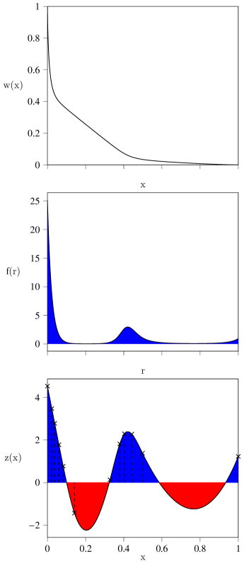
Fig. 11: Internal function constructs $z$ (zero-integral spline), $f$ (Bayes density) and $W$ (WT). The plot displays the underlying spline knots of $z$.

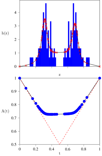
Fig. 12: PF $A$ and target density $h$. The knots represent the function values at the $t_{i}$’s grid defined in alg:h-from-a.

Fig. 13(a) shows the Bayesian posterior distribution of SBEVC PFs, using the previous PLL result as an initial guess for the MCMC sampling. We drew a million random observations from the posterior distribution. The job was divided into 100 [51] tasks corresponding to MCMC runs with 100 independent walkers [22], each one generating 200 observations, with a burn-in period of 100. The confidence interval turned out to be wider than expected but preserving the overall shape. In turn, Fig. 13(b) shows the COBS model, which happens to have a very different shape from Fig. 13(a), lacking a flat central region. Fig. 13(b) demonstrates that COBS captures symmetry well. Interestingly, the COBS model falls outside the confidence interval in Fig. 13(a), indicating that SBEVC and COBS have very different approaches to data fitting.

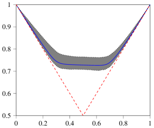
(a) Posterior sample for SBEVC

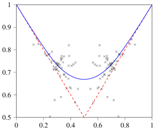
(b) PF for COBS

Fig. 13: On the left, pointwise confidence interval (98%) and mean of the posterior PFs sample from the MCMC simulation. On the right, the COBS PF model fitting the empirical graph $(Z_{i},T_{i})$.

Fig. 14 shows the corresponding sample-density plots for SBEVC and COBS after reversal of the survival transformation. The pdfs capture the presence of lower tail dependence and the absence of upper tail dependence in both cases. The correlation is also very similar. However, there is a remarkable density gap in Fig. 14(a) in the region surrounding the diagonal $\{u=v\}$ that is not present in Fig. 14(b). This is how the presence or absence in Fig. 13 of a flat region translates to pdfs. Consequently, SBEVC and COBS disagree when evaluating the chances of BMs involving similar masses. However, the fitted observations from $\widetilde{\mathcal{D}}_{\text{cop}}$ seem to better support SBEVC’s hypothesis than COBS’.

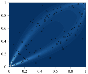
(a) SBEVC

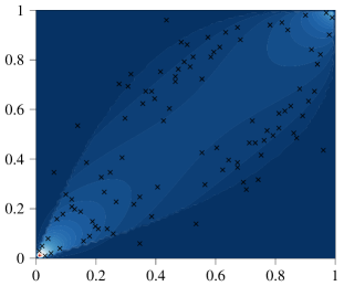
(b) COBS

Fig. 14: Final copula pdfs for SBEVC and COBS after reversal of the survival transformation. The data points shown belong to the $\widetilde{\mathcal{D}}_{\text{cop}}$ dataset.

Table 4 encompasses log-likelihood values of SBEVC and COBS on $\widetilde{\mathcal{D}}_{\text{surv}}$. The SBEVC model considered is the original asymmetrical one in Fig. 12. Given the apparent similarity between Fig. 13(b) and the instances in Fig. 5, we included a Gumbel copula fitted via MLE in the comparison. The results confirm the superiority of SBEVC to COBS and the parametric model by a large margin. The latter is the least fit of the three, just below COBS.

$\mathrm{SBEVC}$	$\mathrm{COBS}$	$\mathrm{Gumbel}(\theta=1.87)$
55.47	33.39	32.48

Table 4: Log-likelihood of different models on the dataset $\widetilde{\mathcal{D}}_{\text{surv}}$.

Joint model

Once fitted both the univariate margin mass model (ZBSs) and the copula models (SBEVC and COBS), the final joint model immediately followed. Fig. 15 plots the original LIGO-Virgo dataset against a random sample generated from each SBEVC and COBS model. The first and second components are the maximum and the minimum, respectively. There are ten times more random samples than original data points, for a total of 500. Fig. 15(a) and Fig. 15(b) show very similar simulations. Both capture three main clusters, concentrated in the regions $[0,20]^{2}$, $[20,40]\times[0,20]$ and $[20,40]^{2}$. It is also worth mentioning that there seems to be a barrier at $\{M_{2}=40\}$; it seems unlikely that giant masses merge. As pointed out by Fig. 14, pictures Fig. 15(a) and Fig. 15(b) slightly differ in BMs with similar masses, being the diagonal just a bit denser in Fig. 15(b).

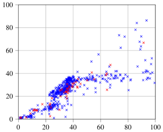
(a) SBEVC

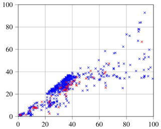
(b) COBS

Fig. 15: Original masses (red) against random samples from SBEVC (blue, on the left) and COBS (blue, on the right).

4 Discussion

SBEVC is fundamentally different from existing EVC estimation approaches. It provides a flexible semiparametric structure, admitting many unconstrained parameters without breaking PF assumptions. Even in the bivariate case, those two feats are difficult to achieve simultaneously [55]. Moreover, retaining complete control of the parameter space opens up exciting possibilities for statistical modelling and data analysis. Indeed, Fig. 7 and Fig. 13(a) represent breakthroughs in EVC theory. Fig. 7 advances the exploration of the PF space with additional smoothing and expressiveness, extending the seminal work by [37] [37]. Fig. 13(a) shows a Bayesian posterior sample analysis of PFs, contributing to solving inferential problems. Nonparametric approaches, lacking a proper structure, depend on specific samples to build models and can only answer a limited array of inferential questions.

The results obtained in Section 3 demonstrate the fitting power of SBEVC on a broad spectrum of EVC configurations coming from parametric models or even random SBEVCs like Fig. 7. Specifically, SBEVC outperforms a similarly-intended nonparametric approach like COBSs [13] on small and medium-sized samples. This superiority does not lie in the number of parameters, similar in both, but in the more efficient fitting strategy by SBEVC, especially when data is scarce. Comparing the top picture in Fig. 12 with Fig. 13(b), we see that SBEVC fits a univariate pdf via MLE relying on exact observations, whereas COBS attempts a constrained regression on points derived from an empirical copula. The latter approach will generally be more sensitive to deviations from the EVC hypothesis, as implied by the fact that some of the fitted points in Fig. 13(b) lie outside the admissible region in Fig. 1(a). Nevertheless, it is remarkable that SBEVC managed to beat COBS in the RMISE metric, not directly targeted by SBEVC, which shows the far-reaching capabilities of MLE.

SBEVCs represent a vast class of EVCs. Two notable copulas fall outside our construction, namely the independence and comonotonic copulas, which correspond to boundary cases of the PF geometry. These limiting cases are usually handled by other means separately and can be approximated in practice through SBEVCs, as demonstrated in Fig. 7. Additionally, [38]’s device could be applied to refine SBEVCs in very low correlation settings. Nonetheless, the construction of SBEVCs holds the key for fitting even more expressive models by replacing ZBSs with neural network architectures [39], perhaps at the expense of losing identifiability and a higher risk of overfitting.

Despite all the previous theoretical and practical arguments favouring SBEVC, the reader may wonder if it is worth the extra execution time and software complexity. After all, COBS can be easily implemented, is already available in R, and provides almost instantaneous results. What is more, some may even question the practical relevance of complying with PF constraints. Unfortunately, there is no definitive answer to those questions: it depends on the user’s goals. The seeming complexity of SBEVC is comparable to that of [32]’s proposal. Theoretical guarantees on the PF are nice to have, ensuring the EVC dependence structure and proper random behaviour in simulation. In most situations, for exploratory data analysis, a compliant nonparametric method like COBS may be the right choice. SBEVC may not be a good option if there are tight time constraints. However, if a more powerful fit is required, data deviates from EVC assumptions, there is not enough data to confidently apply COBS, or one would wish to explore inferential aspects, then SBEVC might be the better, if not the only one.

5 Conclusions

We have introduced a novel semiparametric approach for estimating bivariate EVCs. To our knowledge, it is the first time such an attempt has been made. SBEVC allows many parameters while complying with PF constraints. The construction harbours an intriguing potential for Bayesian inference and deep learning. SBEVCs represent a vast class of EVCs, encompassing a broad spectrum of dependence strengths and asymmetries. Several SBEVCs’ convergence and association properties have been explored. We have also presented all the algorithms required for effectively and efficiently running the estimation process. The SS shows promising results for SBEVC in a wide range of sampling configurations. Specifically, SBEVC produces significantly lower RMISE values than COBS. Finally, the case study demonstrates that SBEVC fits small samples more flexibly than conventional methods.

Appendix A Proofs

Proof of prop:A-W-equivalence.

Let $W$ be as defined above. We will see that $A$ as defined in (7) is a PF with the additional constraint above.

First, note that $t(0)=0$, $t(1)=1$. By continuity of $W$, this implies that $\text{Ran}(t)=[0,1]$. Then, for $t(x)$ to be an automorphism of $[0,1]$, it suffices to see that it is one-to-one. Let us suppose that $t(x_{1})=t(x_{2})$ for some $x_{1},x_{2}\in[0,1]$, $x_{1}<x_{2}$. Then, $W(x_{2})-W(x_{1})=x_{2}-x_{1}>0$, which leads to a contradiction with $W$ being non-increasing. Therefore, $t(x)$ is an automorphism of $[0,1]$, so $A$ in (7) is well-defined as a function of a single variable $t\in[0,1]$.

Next, letting the support lines $t_{+}(x)\equiv t(x)$ and $t_{-}(x)\equiv 1-t(x)$, it is easy to check that $t_{\pm}(x)=\left(1\pm x\mp W(x)\right)/2$ and, since both $x$ and $W(x)$ are non-negative (otherwise $W$ would not be non-increasing, with Ran(W) = $[0,1]$), we may conclude $A(t(x))\geq\max\{t_{+}(x),t_{-}(x)\}$. Furthermore, $A(t(x))>1-t(x)$ for all $x\in(0,1]\supset(0,1/2]$.

Since $W^{\prime}(x)\leq 0$ and $W^{\prime\prime}(x)\geq 0$, it follows that $A^{\prime\prime}(t)\geq 0$, for all $t\in(0,1)$, and hence $A$ is convex. This finishes the proof that (7) defines a PF such that $A(t)>1-t$, for all $t\in(0,1/2]$.

Conversely, let $A$ be a PF with the latter additional constraint. We will similarly show that $W$ as defined in (8) is 2-monotone and satisfies $W(0)=1$ and $W(1)=0$.

First, note that $x(0)=0$ and $x(1)=0$. By continuity of $A$, this implies that $\text{Ran}(x)=[0,1]$. Then, for $x(t)$ to be an automorphism, it suffices to see that $x(t)$ is one-to-one. Let us suppose that $x(t_{1})=x(t_{2})$ for some $t_{1},t_{2}\in[0,1]$, $t_{1}<t_{2}$. This implies that $[A(t_{2})-A(t_{1})]/(t_{2}-t_{1})=-1$ and, since $A$ is convex, we must conclude that $A(t)=1-t$ for all $t\in(t_{1},t_{2}]$. Clearly, $t_{2}\leq 1/2$, because $1-t<t$ if $t>1/2$ and, on the other hand, $A(t)\geq\max\{t,1-t\}$. Therefore, $(t_{1},t_{2}]\subset(0,1/2]$, which leads to a contradiction with $A(t)>1-t$ over $(0,1/2]$. Hence, $x(t)$ must be one-to-one and, all in all, an automorphism of $[0,1]$. This, in turn, means that $W$ in (8) is well-defined as a function of a single variable in $[0,1]$.

Next, it is easy to check both $W(0)=1$ and $W(1)=0$, bearing in mind that $A(0)=A(1)=1$.

Since $A(t)>1-t$ for $t\in(0,1/2]$ and $A$ being convex, we have $A^{\prime}(t)>-1$ and the denominator in both (11) and (12) is well-defined. Moreover, $A^{\prime}(t)\leq 1$, otherwise we would have $A(1-\epsilon)<1-\epsilon$ for a sufficiently small $\epsilon$. Therefore, $W^{\prime}(x)\leq x$ for all $x\in(0,1)$. On the other hand, the convexity of $W$ follows directly from $A^{\prime\prime}(t)\geq 0$.

Finally, the derivatives (9) and (10), on the one hand, and  (11) and (12), on the other, directly follow by differentiating (7) and (8). ∎

Proof of prop:fn-converge-imply-wn-converge.

It suffices to check that, for all $x\in[0,1]$,

$$\lvert W(x)-W_{n}(x)\rvert =\left\lvert\int_{0}^{1}\left(1-\frac{x}{r}\right)_{+}[f(r)-f_{n}(r)]\ dr\right\rvert$$

$$\leq\int_{0}^{1}\lvert f(r)-f_{n}(r)\rvert\ dr\,,$$

where $(\cdot)_{+}$ denotes the non-negative part of the argument, and then apply Scheffé’s theorem (27). Similarly, considering the compact subset $[x_{0},1]$, for some $x_{0}>0$, we have, for all $x\in[x_{0},1]$, $\lvert W^{\prime}(x)-W_{n}^{\prime}(x)\rvert\leq 2\ d_{\text{TV}}(f,f_{n})/x_{0}$. ∎

Proof of prop:graph-convergence.

It follows from the equivalence between uniform convergence and function graph convergence [56] for functions with compact domain and range. Since the $W_{n}$’s uniformly converge to a continuous function $W$, the sequence of the graphs of the $W_{n}$’s has its limit in the graph of $W$. Then, note that the graphs of $A_{n}$ and $A$ are affine transformations (7) of the graphs of $W_{n}$ and $W$, respectively. This ensures, by continuity, that the graphs of the $A_{n}$’s tend to that of $A$. Finally, graph convergence for the $A_{n}$’s implies uniform convergence to $A$ itself.

The result for the first derivatives follows similarly. Instead of an affine map, the functions mapping the graph of $W$ to that of $A$ and vice versa are, respectively,

$$\mathbb{T}(x,w^{\prime})=\left[t(x),\frac{1+w^{\prime}}{1-w^{\prime}}\right]\,,$$

$$\mathbb{X}(t,a^{\prime})=\left[x(t),\frac{a^{\prime}-1}{a^{\prime}+1}\right]\,.$$

Both are the inverse of one another because of (9) and (11). Both functions are continuous. Hence, they preserve compactness and graph convergence.

To see that $\{A_{n}^{\prime}\}_{n=1}^{\infty}$ compactly converges to $A^{\prime}$, consider any compact set $\mathcal{K}=[t_{0},1]$, for $t_{0}>0$. Then, consider the sequence of restricted function graphs $\{\mathcal{G}[A_{n}^{\prime}|_{\mathcal{K}}]\}_{n=1}^{\infty}$ and apply $\mathbb{X}$ to every element to obtain another sequence $\{\mathcal{G}[W_{n}^{\prime}|_{\mathcal{\mathbb{X}(K)}}]\}_{n=1}^{\infty}$. Now, $\mathbb{X}(\mathcal{K})$ is a compact set, so $W_{n}^{\prime}|_{\mathcal{\mathbb{X}(K)}}$ uniformly converges to $W^{\prime}|_{\mathcal{\mathbb{X}(K)}}$ and, because of  [56], the graph sequence approaches $\mathcal{G}[W^{\prime}|_{\mathcal{\mathbb{X}(K)}}]$. The argument finishes by noting that, since $\mathbb{T}$ is continuous and since $\mathbb{T}(\mathcal{G}[W_{n}^{\prime}|_{\mathcal{\mathbb{X}(K)}}])=\mathcal{G}[A_{n}^{\prime}|_{\mathcal{K}}]$ and $\mathbb{T}(\mathcal{G}[W^{\prime}|_{\mathcal{\mathbb{X}(K)}}])=\mathcal{G}[A^{\prime}|_{\mathcal{K}}]$, the graphs of the $A_{n}^{\prime}|_{\mathcal{K}}$’s tend to that of $A^{\prime}|_{\mathcal{K}}$. ∎

Proof of prop:convergence-tvd-pdfs.

First, note that continuity ensures that the limit $p$ is also bounded by the same $K$. Denoting $I_{q}=\int_{0}^{1}e^{q}$, some easy calculations show that

$$|f(x)-f_{n}(x)|\leq\frac{e^{p(x)}|I_{p}-I_{p_{n}}|+I_{p}\ |e^{p(x)}-e^{p_{n}(x)}|}{I_{p}\ I_{p_{n}}}\,.$$

Now, the integrals are bounded, namely $e^{-K}\leq I_{q}\leq e^{K}$. On the other hand, $|e^{p(x)}-e^{p_{n}(x)}|\leq e^{K}|p(x)-p_{n}(x)|$, using the mean value theorem and the fact that both functions are bounded by $K$. All in all,

$$|f(x)-f_{n}(x)|\leq e^{4K}\left(\int_{0}^{1}|p(y)-p_{n}(y)|\ dy+|p(x)-p_{n}(x)|\right)\,.$$

Integrating both sides of the last inequality and using Jensen’s inequality, we finally get $d_{\text{TV}}(f,f_{n})\leq e^{4K}\lVert p-p_{n}\rVert_{2}$. ∎

Proof of cor:convergence-partial-derivatives.

It follows from all the previous convergence results and the form of the partial derivative of an EVC [19, 16], where all the terms uniformly converge on compact sets. ∎

Proof of alg:estimate-W.

Let us set aside the normalization by $\bar{W}_{0}$ for a moment. Clearly, $\bar{W}_{i}^{\prime\prime}$ is a straight approximation for $W_{\bm{\theta}}^{\prime\prime}(r_{i})$. It only remains to check that (31) and (30) provide good approximations for $W_{\bm{\theta}}(r_{i})$ and $W_{\bm{\theta}}^{\prime}(r_{i})$, respectively. It suffices to see that

$$\bar{W}_{i}^{\prime}=\sum_{j=i}^{n}\bar{W}_{j}^{\prime}-\bar{W}_{j+1}^{\prime}=-\sum_{j=i}^{n}Q_{j}\approx-\int_{r_{i}}^{1}\frac{f_{\bm{\theta}}(r)}{r}\ dr$$

and, taking into account (19),

$$\bar{W}_{i} =\sum_{j=i}^{n}\bar{W}_{j}-\bar{W}_{j+1} =\sum_{j=i}^{n}s_{j}\bar{W}_{j}^{\prime}-s_{j+1}\bar{W}_{j+1}^{\prime}+P_{j}$$

$$=s_{i}\bar{W}_{i}^{\prime}+\sum_{j=i}^{n}P_{j} \approx r_{i}W_{\bm{\theta}}^{\prime}(r_{i})+\int_{r_{i}}^{1}f_{\bm{\theta}}(r)\ dr\,,$$

where we have used that $P_{i}$ and $Q_{i}$ are the trapezoidal rule approximations for $\int_{r_{i}}^{r_{i+1}}f_{\bm{\theta}}$ and $\int_{r_{i}}^{r_{i+1}}f_{\bm{\theta}}(r)/r\ dr$, respectively. Also, implicit in the previous argument was the approximation $s_{0}=\epsilon\approx 0$, used to avoid infinite values. Finally, the last normalization step aims to stabilize the estimation process against numerical errors, enforcing the constraint $W_{\bm{\theta}}(0)=1$. ∎

Proof of alg:h-from-a.

The rationale of the algorithm is relatively straightforward. Equation (32) mimics (28), where $A_{\bm{\theta}}$ and its derivatives are evaluated over $t_{i}$ indirectly through equations (7), (9) and (10), requiring only the $x_{i}$’s and approximations of $W_{\bm{\theta}}$ and its derivatives at those points. On the other hand, the reader can easily check that $h_{\bm{\theta}}(0)=h_{\bm{\theta}}(1)=0$, considering all the constraints imposed by SBEVC: $A_{\bm{\theta}}^{\prime}(0^{+})=-1$, $A_{\bm{\theta}}^{\prime}(1^{-})=1$ and $f_{\bm{\theta}}(x)>0$ for all $x\in[0,1]$, among others. The case at the $0$ endpoint is not trivial, but nearly so. After simplification, we arrive at

$$h_{\bm{\theta}}(0)=2f_{\bm{\theta}}(0)\lim_{x\rightarrow 0^{+}}\frac{1+x-W_{\bm{\theta}}(x)}{x(1-W_{\bm{\theta}}^{\prime}(x))^{3}}\,.$$

Repeatedly applying L’Hôpital’s rule, we can check that the denominator tends to zero and, eventually, the whole limit also tends to zero. Finally, the step involving the integral ensures $\int_{0}^{1}\tilde{h}=1$, making a $\tilde{h}$ a true pdf, which was not automatically granted by the linear interpolation strategy. ∎

references type=article or type=book or type=incollection or type=inproceedings or type=manual or type=thesis

resources type=software or type=online

References

- [1] B. P. Abbott et al. “Observation of Gravitational Waves from a Binary Black Hole Merger” In Physical Review Letters 116.6 American Physical Society (APS), 2016 DOI: 10.1103/physrevlett.116.061102
- [2] R. Abbott et al. “Population Properties of Compact Objects from the Second LIGO–Virgo Gravitational-Wave Transient Catalog” In The Astrophysical Journal Letters 913.1 American Astronomical Society, 2021, pp. L7 DOI: 10.3847/2041-8213/abe949
- [3] G. E. Alefeld, F. A. Potra and Yixun Shi “Algorithm 748: enclosing zeros of continuous functions” In ACM Transactions on Mathematical Software 21.3 Association for Computing Machinery (ACM), 1995, pp. 327–344 DOI: 10.1145/210089.210111
- [4] Argo Project “Argo CD” URL: https://argoproj.github.io/argo-cd/
- [5] Tomáš Bacigál “On Some Applications of Williamson’s Transform in Copula Theory” In Advances in Intelligent Systems and Computing Springer International Publishing, 2017, pp. 21–30 DOI: 10.1007/978-3-319-59306-7˙3
- [6] Carl Boor “Spline Basics” In Handbook of Computer Aided Geometric Design Elsevier, 2002, pp. 141–163 DOI: 10.1016/b978-044451104-1/50007-1
- [7] Eric Bouyé et al. “Copulas for Finance - A Reading Guide and Some Applications” In SSRN Electronic Journal Elsevier BV, 2000 DOI: 10.2139/ssrn.1032533
- [8] Richard H. Byrd, Peihuang Lu, Jorge Nocedal and Ciyou Zhu “A Limited Memory Algorithm for Bound Constrained Optimization” In SIAM Journal on Scientific Computing 16.5 Society for Industrial & Applied Mathematics (SIAM), 1995, pp. 1190–1208 DOI: 10.1137/0916069
- [9] P. Capéraà, A. L. Fougères and C. Genest “A nonparametric estimation procedure for bivariate extreme value copulas” In Biometrika 84.3 Oxford University Press (OUP), 1997, pp. 567–577 DOI: 10.1093/biomet/84.3.567
- [10] Jorge Cervantes-Cota, Salvador Galindo-Uribarri and George Smoot “A Brief History of Gravitational Waves” In Universe 2.3 MDPI AG, 2016, pp. 22 DOI: 10.3390/universe2030022
- [11] A. Charpentier, A. L. Fougères, C. Genest and J. G. Nešlehová “Multivariate Archimax copulas” In Journal of Multivariate Analysis 126 Elsevier BV, 2014, pp. 118–136 DOI: 10.1016/j.jmva.2013.12.013
- [12] R. M. Corless et al. “On the LambertW function” In Advances in Computational Mathematics 5.1 Springer ScienceBusiness Media LLC, 1996, pp. 329–359 DOI: 10.1007/bf02124750
- [13] Eric Cormier, Christian Genest and Johanna Nešlehová “Using B-splines for nonparametric inference on bivariate extreme-value copulas” In Extremes 17.4 Springer ScienceBusiness Media LLC, 2014, pp. 633–659 DOI: 10.1007/s10687-014-0199-4
- [14] Data Mechanics “Docker image for Apache Spark” URL: https://hub.docker.com/r/datamechanics/spark
- [15] Docker, Inc. “Docker” URL: https://www.docker.com/
- [16] Gabriel Doyon “On Densities of Extreme Value Copulas”, 2013
- [17] J. J. Egozcue, J. L. Díaz–Barrero and V. Pawlowsky–Glahn “Hilbert Space of Probability Density Functions Based on Aitchison Geometry” In Acta Mathematica Sinica, English Series 22.4 Springer ScienceBusiness Media LLC, 2006, pp. 1175–1182 DOI: 10.1007/s10114-005-0678-2
- [18] John H. J. Einmahl and Johan Segers “Maximum empirical likelihood estimation of the spectral measure of an extreme-value distribution” In The Annals of Statistics 37.5B Institute of Mathematical Statistics, 2009 DOI: 10.1214/08-aos677
- [19] Patrick Eschenburg “Properties of extreme-value copulas”, 2013
- [20] Amèlie Fils-Villetard, Armelle Guillou and Johan Segers “Projection estimators of Pickands dependence functions” In Canadian Journal of Statistics 36.3 Wiley, 2008, pp. 369–382 DOI: 10.1002/cjs.5550360303
- [21] Andrea Fontanari, Pasquale Cirillo and Cornelis W. Oosterlee “Lorenz-generated bivariate Archimedean copulas” In Dependence Modeling 8.1 Walter de Gruyter GmbH, 2020, pp. 186–209 DOI: 10.1515/demo-2020-0011
- [22] Daniel Foreman-Mackey, David W. Hogg, Dustin Lang and Jonathan Goodman “emcee: The MCMC Hammer” In Publications of the Astronomical Society of the Pacific 125.925 IOP Publishing, 2013, pp. 306–312 DOI: 10.1086/670067
- [23] Christian Genest and Johanna Nešlehová “When Gumbel met Galambos” In Copulas and Dependence Models with Applications Springer International Publishing, 2017, pp. 83–93 DOI: 10.1007/978-3-319-64221-5˙6
- [24] Christian Genest, Johanna Nešlehová and Jean-François Quessy “Tests of symmetry for bivariate copulas” In Annals of the Institute of Statistical Mathematics 64.4 Springer ScienceBusiness Media LLC, 2011, pp. 811–834 DOI: 10.1007/s10463-011-0337-6
- [25] Pierre Georges et al. “Multivariate Survival Modelling: A Unified Approach with Copulas” In SSRN Electronic Journal Elsevier BV, 2001 DOI: 10.2139/ssrn.1032559
- [26] Ghorbal, Genest and Nešlehová “On the Ghoudi, Khoudraji, and Rivest test for extreme-value dependence” In Canadian Journal of Statistics 37.4 Wiley, 2009, pp. 534–552 DOI: 10.1002/cjs.10034
- [27] Google Cloud Platform “Spark Operator” URL: https://operatorhub.io/operator/spark-gcp
- [28] Gordon Gudendorf and Johan Segers “Extreme-Value Copulas” In Copula Theory and Its Applications Springer Berlin Heidelberg, 2010, pp. 127–145 DOI: 10.1007/978-3-642-12465-5˙6
- [29] Gordon Gudendorf and Johan Segers “Nonparametric estimation of multivariate extreme-value copulas” In Journal of Statistical Planning and Inference 142.12 Elsevier BV, 2012, pp. 3073–3085 DOI: 10.1016/j.jspi.2012.05.007
- [30] Simon Guillotte and François Perron “Polynomial Pickands functions” In Bernoulli 22.1 Bernoulli Society for Mathematical StatisticsProbability, 2016, pp. 213–241 DOI: 10.3150/14-bej656
- [31] Sándor Guzmics and Georg Ch. Pflug “A new extreme value copula and new families of univariate distributions based on Freund’s exponential model” In Dependence Modeling 8.1 Walter de Gruyter GmbH, 2020, pp. 330–360 DOI: 10.1515/demo-2020-0018
- [32] José Miguel Hernández-Lobato and Alberto Suárez “Semiparametric bivariate Archimedean copulas” In Computational Statistics & Data Analysis 55.6 Elsevier BV, 2011, pp. 2038–2058 DOI: 10.1016/j.csda.2011.01.018
- [33] Marius Hofert, Ivan Kojadinovic, Martin Maechler and Jun Yan “copula: Multivariate Dependence with Copulas” R package version 1.0-1, 2020 URL: https://CRAN.R-project.org/package=copula
- [34] Ivan Kojadinovic and Jun Yan “Modeling Multivariate Distributions with Continuous Margins Using the copula R Package” In Journal of Statistical Software 34.9, 2010, pp. 1–20 URL: https://www.jstatsoft.org/v34/i09/
- [35] Javier Rojo Jiménez, Enrique Villa-Diharce and Miguel Flores “Nonparametric Estimation of the Dependence Function in Bivariate Extreme Value Distributions” In Journal of Multivariate Analysis 76.2 Elsevier BV, 2001, pp. 159–191 DOI: 10.1006/jmva.2000.1931
- [36] Jun Yan “Enjoy the Joy of Copulas: With a Package copula” In Journal of Statistical Software 21.4, 2007, pp. 1–21 URL: https://www.jstatsoft.org/v21/i04/
- [37] N. Kamnitui, C. Genest, P. Jaworski and W. Trutschnig “On the size of the class of bivariate extreme-value copulas with a fixed value of Spearman's rho or Kendall's tau” In Journal of Mathematical Analysis and Applications 472.1 Elsevier BV, 2019, pp. 920–936 DOI: 10.1016/j.jmaa.2018.11.057
- [38] A. Khoudraji “Contributions à l’étude des copules et à la modélisation des valeurs extrêmes bivariées”, 1995
- [39] Chun Kai Ling, Fei Fang and J. Zico Kolter “Deep Archimedean Copulas” In 34th Conference on Neural Information Processing Systems (NeurIPS 2020), 2020 arXiv:2012.03137 [cs.LG]
- [40] Jitka Machalová, Renáta Talská, Karel Hron and Aleš Gába “Compositional splines for representation of density functions” In Computational Statistics 36.2 Springer ScienceBusiness Media LLC, 2020, pp. 1031–1064 DOI: 10.1007/s00180-020-01042-7
- [41] Dougal Maclaurin, David Duvenaud and Ryan P. Adams “Autograd: Effortless gradients in numpy” In ICML 2015 AutoML Workshop 238, 2015, pp. 5
- [42] G. Marcon et al. “Multivariate nonparametric estimation of the Pickands dependence function using Bernstein polynomials” In Journal of Statistical Planning and Inference 183 Elsevier BV, 2017, pp. 1–17 DOI: 10.1016/j.jspi.2016.10.004
- [43] Marius Hofert and Martin Mächler “Nested Archimedean Copulas Meet R: The nacopula Package” In Journal of Statistical Software 39.9, 2011, pp. 1–20 URL: https://www.jstatsoft.org/v39/i09/
- [44] Alexander J. McNeil and Johanna Nešlehová “Multivariate Archimedean copulas, d-monotone functions and 1-norm symmetric distributions” In The Annals of Statistics 37.5B Institute of Mathematical Statistics, 2009, pp. 3059–3097 DOI: 10.1214/07-aos556
- [45] Alexander J. McNeil and Johanna Nešlehová “From Archimedean to Liouville copulas” In Journal of Multivariate Analysis 101.8 Elsevier BV, 2010, pp. 1772–1790 DOI: 10.1016/j.jmva.2010.03.015
- [46] James Pickands “Multivariate extreme value distribution” In Proceedings 43th, Session of International Statistical Institution, 1981, 1981
- [47] Jean-François Quessy and Othmane Kortbi “Minimum-distance statistics for the selection of an asymmetric copula in Khoudraji's class of models” In Statistica Sinica Institute of Statistical Science, 2016 DOI: 10.5705/ss.202014.0082
- [48] Schmitz “Copulas and Stochastic Processes”, 2003 URL: https://d-nb.info/972691669/34
- [49] Larry I. Schumaker “On Shape Preserving Quadratic Spline Interpolation” In SIAM Journal on Numerical Analysis 20.4 Society for Industrial & Applied Mathematics (SIAM), 1983, pp. 854–864 DOI: 10.1137/0720057
- [50] Serrano “Modelling Multivariate Dependencies with Semiparametric Archimedean Copulas”, 2016, pp. 172 URL: http://hdl.handle.net/10486/676101
- [51] The Apache Software Foundation “Spark”, 2021 URL: https://spark.apache.org/
- [52] The Cloud Native Computing Foundation “Kubernetes” URL: https://kubernetes.io/
- [53] The Minikube Community “minikube” URL: https://minikube.sigs.k8s.io/
- [54] Alexandre B. Tsybakov “Introduction to Nonparametric Estimation” Springer New York, 2009 DOI: 10.1007/b13794
- [55] Sabrina Vettori, Raphaël Huser and Marc G. Genton “A comparison of dependence function estimators in multivariate extremes” In Statistics and Computing 28.3 Springer ScienceBusiness Media LLC, 2017, pp. 525–538 DOI: 10.1007/s11222-017-9745-7
- [56] William C. Waterhouse “Uniform Convergence and Graph Convergence” In The American Mathematical Monthly 83.8 JSTOR, 1976, pp. 641 DOI: 10.2307/2319894