Phase diagram of the Hubbard model on a honeycomb lattice:
A cluster slave-spin study

Abstract

The cluster slave-spin method is implemented to research the ground state properties of the honeycomb lattice Hubbard model with doping $\delta$ and coupling $U$ being its parameters. At half-filling, a single direct and continuous phase transition between the semi-metal and antiferromagnetic (AFM) insulator is found at $U_{\text{AFM}}=2.43t$ that is in the Gross-Neveu-Yukawa universality class, where a relation between the staggered magnetization $M$ and the AFM energy gap $\Delta_{\text{AFM}}$ is established as $M\propto\Delta_{\text{AFM}}$, compared to $M\propto\Delta_{\text{AFM}}(\ln{\Delta_{\text{AFM}}})^{2}$ in the square lattice case. A first-order semi-metal to the underlying paramagnetic (PM) insulator Mott transition is corroborated at $U_{\text{Mott}}=8.36t$, which is responsible for a broad crossover around $U_{c}=5.4t$ between the weak- and strong-coupling regimes in the AFM state that increases with $\delta$, in contrast to the square lattice case. In the doped system, the compressibility $\kappa$ near the van Hove singularity at $\delta=1/4$ is suppressed substantially by the interaction before the semi-metal to AFM transition occurs, whereas $\kappa$ near the Dirac points is very close to the noninteracting one, indicating that the Dirac cone structure of the energy dispersion is rather robust. An overall phase diagram in the $U$-$\delta$ plane is presented, consisting of four regimes: the AFM insulator at $\delta=0$ for $U>U_{\text{AFM}}$, the AFM metal with compressibility $\kappa>0$ or $\kappa<0$, and the PM semi-metal, and the AFM metal with $\kappa<0$ only exists in an extremely small area near the phase boundary between the AFM and PM state.

I INTRODUCTION

The Hubbard Hamiltonian Hubbard (1963); *Hubbard1964 has been acting over decades as a prototypical model for the description of interacting electrons. In spite of its seeming simplicity, this model captures a rich phenomenology of strongly-correlated electrons such as metallic-insulating, nonmagnetic-antiferromagnetic and normal-superconducting phase transitions and can not be solved exactly in more than one dimensions, which necessitates some nonperturbative approaches to deal with the strong-coupling aspect of the model White et al. (1989); Qin et al. (2021). In this paper, we will focus on the one-band Hubbard model defined on a honeycomb (hexagon) network (Bravais lattice for graphene), which is bipartite and admits the antiferromagnetism (AFM) in the strong coupling limit. This model has a linear free electron energy dispersion with nodal gapless points at the corners of the Brillouin zone, leading to the so-called Dirac semi-metal. Due to the gapless Dirac points, there is a nontrivial semi-metal to antiferromagnetic insulator (AFMI) transition at a finite coupling strength at half-filling, which makes this model an ideal playground to research the interaction-driven semi-metal to AFMI transition. Up till now, many numerical and analytical methods have been applied to the half-filled system to study this transition and its critical behaviors. Large scale quantum Monte Carlo (QMC) simulations of $648$ sites predict a spin liquid state in a range of interaction $3.5t<U<4.3t$, beyond which the AFM sets in Meng et al. (2010), and this argument was supported by some numerical works Hohenadler et al. (2011, 2012a, 2012b); Zheng et al. (2011). Nevertheless, this picture was disputed by many other numerical studies Otsuka et al. (2016); Raczkowski et al. (2020); Assaad and Herbut (2013); Paiva et al. (2005); Yamada (2016); Sorella and Tosatti (1992); Sorella et al. (2012); Ostmeyer et al. (2020, 2021), especially those using the same method containing up to $2592$ sites Sorella et al. (2012); Otsuka et al. (2016) and $20808$ sites Ostmeyer et al. (2020, 2021). By means of cluster dynamical mean-field theory, variational cluster approximation, and cluster dynamical impurity approximation, Hassan et al. Hassan and Sénéchal (2013) showed that the results are dependent on the shape and size of the clusters, and they claimed that only the system with two bath orbits per cluster boundary site is able to describe the correct behavior and found that the Mott transition for the spin liquid state is actually preempted by the AFM long-range order. Though the early variational cluster calculations Seki and Ohta (2012) argued that the single-particle gap opens at an infinitesimal value of $U$, recent dynamical cluster approximation study found that this spurious excitation gap is due to the violation of the translation symmetry of the system and the cluster with one bath orbital per cluster site is sufficient for the description of the short-range correlations within the honeycomb unit cell Liebsch and Wu (2013a). A recent density matrix embedding theory study revealed a paramagnetic insulating state with possible hexagonal cluster state at intermediate coupling strength whose stability is highly cluster and lattice size dependent, and this state is nonexistent in the thermodynamic limit, signaling no intermediate state in the half-filled Hubbard model on a honeycomb lattice Chen et al. (2014). In addition, a two-particle self-consistent study presented a semi-metal to AFMI transition and proved that the transition from a semi-metal to spin liquid phase is forestalled by this transition Arya et al. (2015). The functional renormalization group theory predicts a critical interaction strength $U=3.8t$ that is consistent with the results from the methods mentioned above, supporting that there is no spin liquid state at intermediate coupling strengths Honerkamp (2008); Raghu et al. (2008).

Based on the charge-spin separation theory Wang et al. (1993); Feng et al. (1993); *Feng_1994; *Feng_2003; *Feng_2004; *Feng_2015; Hassan and de’ Medici (2010), the $U(1)$ slave-spin method has been proposed to cope with the Mott transition in multi-orbital systems Yu and Si (2012), which is very economical computationally because only $2M$ slave spins need to be introduced per site with $M$ being the number of orbits. This method can not only reproduce the Gutzwiller factor $g_{t}=\frac{1-x-2d}{1-x-(1-x)^{2}/2}(\sqrt{x+d}+\sqrt{d})^{2}$, but also capture the right noninteracting behaviors at $U=0$ because of an extra orbital-dependent chemical potential in the spinon Hamiltonian, which makes it a powerful method to deal with the strong-coupling systems Lee and Lee (2017). Then, a cluster slave-spin approach was developed to address strongly correlated systems to take the short-range charge fluctuations into account Lee and Lee (2017) and has been employed to solve the square lattice Hubbard model to obtain an overall ground state phase diagram in the parameter space of doping $\delta$ and interaction $U$ Zeng et al. (2021). In the present work, we apply the same method with the Lanczos exact-diagonalization as the slave-spin cluster solver to the honeycomb lattice Hubbard model to study its ground state properties, including the quantum critical behavior in the vicinity of the interaction-driven semi-metal to AFMI transition at half-filling and an overall phase diagram in the whole $U$-$\delta$ plane. Our motivation is two-fold: (i) Because the results of this model is shown to be highly dependent on the size of the lattice adopted for QMC simulations, as well as the size and shape of the clusters used within various cluster approximations, more results from different approaches ought to be included and compared with each other. (ii) Away from half-filling, much attention was paid to the 1/4-doping, where the free density of states shows a van Hove singularity of logarithmic type, favoring an instability towards superconductivity in the weak interaction regime Gu et al. (2013); Wang et al. (2012); Nandkishore et al. (2012), whereas an overall $U$-$\delta$ phase diagram pertaining to the magnetism is still absent.

In the honeycomb lattice Hubbard model, we find that the first-order Mott transition occurs at $U_{\text{Mott}}=8.36t$ in the half-filled PM state, characterized by discontinuities and hystereses in all quantities, and transforms into a broad crossover in the AFM state because of long range AFM correlations. Besides, the phase separation, manifested by a negative compressibility, has been observed in a region near the phase boundary $\delta_{M}(U)$ between the AFM and PM state and at intermediate couplings, whose area is much smaller compared to the square lattice Hubbard model Zeng et al. (2021). Finally, a phase diagram in the $U$-$\delta$ plane is presented, consisting of four regimes: AFMI, AFM metal with positive and negative compressibility, and the PM semi-metal.

The rest of this paper is organized as follows. In Sec. II, we reintroduce the cluster slave-spin mean-field theory Lee and Lee (2017); Zeng et al. (2021) and implement it in the honeycomb lattice Hubbard model by making use of two- and six-site cluster approximations. In Sec. III.1, for the half-filled system, an analytical relation between the staggered magnetization $M$ and the AFM energy gap $\Delta_{\text{AFM}}$ in the vicinity of the semi-metal to AFMI transition is established, and the first-order Mott transition at $U_{\text{Mott}}=8.36t$ is observed in the PM state. In Sec. III.2, the results of finite doping cases obtained by two- and six-site clusters are discussed thoroughly, and we find that the two-site cluster is inadequate to capture the AFM transition appropriately because it violates the symmetry of the honeycomb lattice. In Sec. IV, the properties of $M$, $\Delta_{\text{AFM}}$, and the compressibility $\kappa$ are combined to show a phase diagram of the model in the $U$-$\delta$ plane.

II Formalism

The standard one-band fermionic Hubbard model Hubbard (1963, 1964) reads

$$H=-t\sum_{\langle i,j\rangle\sigma}(c_{i\sigma}^{\dagger}c_{j\sigma}+\mbox{\sc h.c.})+U\sum_{i}n_{i\uparrow}n_{i\downarrow}-\mu\sum_{i\sigma}n_{i\sigma}\;,$$ (1)

where $t$, $U$, $\mu$ are the nearest hopping constant, the on-site Coulomb repulsion energy and the chemical potential, respectively. The sum $\langle i,j\rangle$ runs over all pairs of nearest-neighbor sites on a honeycomb lattice, and $c_{i\sigma}^{\dagger}$ is the creation operator of the electron at site $i$ with spin $\sigma=\uparrow,\,\downarrow$, and the number operator $n_{i\sigma}=c_{i\sigma}^{\dagger}c_{i\sigma}$. Hereafter, we use $t=1$ as the unit of energy.

In the U(1) slave-spin method Yu and Si (2012), an electron operator is factorized into a slave-spin operator ($S=\tfrac{1}{2}$) and a fermionic spinon operater, describing the charge and spin degrees of freedoms of an electron, respectively:

$$c^{\dagger}_{\alpha}\equiv S^{\dagger}_{\alpha}f^{\dagger}_{\alpha}\;,$$ (2)

on account of which the original Hillbert space with basis $\{|0\rangle,|1\rangle\}$ is enlarged to $\{|n^{f}_{\alpha},S^{z}_{\alpha}\rangle\}=\{|0,-\tfrac{1}{2}\rangle,|1,\tfrac{1}{2}\rangle,|0,\tfrac{1}{2}\rangle,|1,-\tfrac{1}{2}\rangle\}$. Thus, an extra constraint needs to be imposed to restrict the Hillbert space to the physical one: $\{|n^{f}_{\alpha},S^{z}_{\alpha}\rangle\}=\{|0,-\tfrac{1}{2}\rangle,|1,\tfrac{1}{2}\rangle\}$,

$$S^{z}_{\alpha}=f^{\dagger}_{\alpha}f_{\alpha}-\tfrac{1}{2}\;.$$ (3)

A gauge degree of freedom must be introduced to incorporate the constraint, signifying that the slave-spin representation is invariant under a local gauge transformation $f^{\dagger}_{\alpha}\to f^{\dagger}_{\alpha}e^{-i\phi_{\alpha}}$ and $S^{\dagger}_{\alpha}\to S^{\dagger}_{\alpha}e^{i\phi_{\alpha}}$, and all physical quantities should be invariant under this U(1) gauge transformation Coleman (1987); Lee and Nagaosa (1992); Feng et al. (1993); Florens and Georges (2004); Senthil (2008).

With the constraint $a^{\dagger}_{\alpha}a_{\alpha}+b^{\dagger}_{\alpha}b_{\alpha}=1$, the slave-spin operator is rewritten in the Schwinger boson representation

$$S^{\dagger}_{\alpha}=a^{\dagger}_{\alpha}b_{\alpha}\;,\;\;\;\;S^{z}_{\alpha}=\frac{1}{2}\left(a^{\dagger}_{\alpha}a_{\alpha}-b^{\dagger}_{\alpha}b_{\alpha}\right)\;.$$ (4)

To ensure the correct non-interacting behaviors, the slave-boson operators need to be dressed as follows Kotliar and Ruckenstein (1986)

$$\tilde{S}^{\dagger}_{\alpha} = P^{+}_{\alpha}a^{\dagger}_{\alpha}b_{\alpha}P^{-}_{\alpha}\;,$$ (5a)

$$P^{\pm}_{\alpha} = \frac{1}{\sqrt{1/2\pm S^{z}_{\alpha}}}\;,$$ (5b)

which can be linearized as follows:

$$\tilde{S}^{\dagger}_{\alpha}\approx\tilde{z}^{\dagger}_{\alpha}+\frac{\langle\tilde{z}^{\dagger}_{\alpha}\rangle\langle S^{z}_{\alpha}\rangle\Delta S^{z}_{\alpha}}{(\tfrac{1}{2})^{2}-\langle S^{z}_{\alpha}\rangle^{2}}\;,$$ (6)

with $\Delta S^{z}_{\alpha}=S^{z}_{\alpha}-\langle S^{z}_{\alpha}\rangle$ and $\tilde{z}^{\dagger}_{\alpha}=a^{\dagger}_{\alpha}b_{\alpha}/[(\tfrac{1}{2})^{2}-\langle S^{z}_{\alpha}\rangle^{2}]^{1/2}$.

Following the recipe of Lee and Lee Lee and Lee (2017), with the local constraints (3) being ensured roughly by two global Lagrange multipliers $\lambda_{I\sigma}$ on sublattices $I=A$ and $B$, Hamiltonian (1) can be cast into the form

$$H^{f}_{\text{MF}} = -tZ\sum_{\langle i,j\rangle\sigma}(a_{i\sigma}^{\dagger}b_{j\sigma}+\textsc{h.c.})$$ (7a)

$$-\sum_{i\sigma}\big{[}(\mu+\lambda_{A\sigma}-\tilde{\mu}_{A\sigma})a_{i\sigma}^{\dagger}a_{i\sigma}$$

$$\hskip 23.00006pt+(\mu+\lambda_{B\sigma}-\tilde{\mu}_{B\sigma})b_{i\sigma}^{\dagger}b_{i\sigma}\big{]}\;,$$

$$H_{n_{c}\text{-site}}^{S} = H^{\lambda}_{n_{c}\text{-site}}+H^{U}_{n_{c}\text{-site}}+H^{K}_{n_{c}\text{-site}}\;,$$ (7b)

where

$$H^{\lambda}_{n_{c}\text{-site}} = \sum_{i_{c}=1,\sigma}^{n_{c}}\lambda_{I\sigma}S_{i_{c}\sigma}^{z}\;,$$ (8a)

$$H^{U}_{n_{c}\text{-site}} = \sum_{i_{c}=1}^{n_{c}}U(S_{i_{c}\sigma}^{z}+\tfrac{1}{2})(S_{i_{c}\bar{\sigma}}^{z}+\tfrac{1}{2})\;,$$ (8b)

$$H^{K}_{\text{2-site}} = \sum_{\sigma}\Big{\{}\epsilon_{\sigma}^{\delta_{1}}(\tilde{z}_{A\sigma}^{\dagger}\tilde{z}_{B\sigma}+\tilde{z}_{B\sigma}^{\dagger}\tilde{z}_{A\sigma})+(\epsilon_{\sigma}^{\delta_{2}}+\epsilon_{\sigma}^{\delta_{3}})$$ (8c)

$$\hskip 20.00003pt\times\big{[}\tilde{z}_{A\sigma}^{\dagger}\langle\tilde{z}_{B\sigma}\rangle+\tilde{z}_{B\sigma}^{\dagger}\langle\tilde{z}_{A\sigma}\rangle+\textsc{h.c.}\big{]}\Big{\}}\;,$$

$$H^{K}_{\text{6-site}} = \sum_{\sigma}\Big{\{}\epsilon_{\sigma}^{\delta_{1}}(\tilde{z}_{1\sigma}^{\dagger}\tilde{z}_{2\sigma}+\tilde{z}_{4\sigma}^{\dagger}\tilde{z}_{5\sigma})$$ (8d)

$$+\epsilon_{\sigma}^{\delta_{2}}(\tilde{z}_{1\sigma}^{\dagger}\tilde{z}_{6\sigma}+\tilde{z}_{3\sigma}^{\dagger}\tilde{z}_{4\sigma})+\epsilon_{\sigma}^{\delta_{3}}(\tilde{z}_{2\sigma}^{\dagger}\tilde{z}_{3\sigma}+\tilde{z}_{5\sigma}^{\dagger}\tilde{z}_{6\sigma})$$

$$+\epsilon_{\sigma}^{\delta_{1}}(\tilde{z}_{3\sigma}^{\dagger}\langle\tilde{z}_{6\sigma}\rangle+\langle\tilde{z}_{3\sigma}^{\dagger}\rangle\tilde{z}_{6\sigma})$$

$$+\epsilon_{\sigma}^{\delta_{2}}(\tilde{z}_{2\sigma}^{\dagger}\langle\tilde{z}_{5\sigma}\rangle+\langle\tilde{z}_{2\sigma}^{\dagger}\rangle\tilde{z}_{5\sigma})$$

$$+\epsilon_{\sigma}^{\delta_{3}}(\tilde{z}_{1\sigma}^{\dagger}\langle\tilde{z}_{4\sigma}\rangle+\langle\tilde{z}_{1\sigma}^{\dagger}\rangle\tilde{z}_{4\sigma})+\textsc{h.c.}\Big{\}}\;.$$

The mean-field Hamiltonian $H_{n_{c}\text{-site}}^{S}$ is a Bose-Hubbard model for two species of bosons, and actually a model of interacting XY spins in a magnetic field Yu and Si (2012). Senthil has systematically investigated the gauge field fluctuations’ effects on charge and spin degrees of freedom of the one-band Hubbard model in the slave-rotor representation Florens and Georges (2004), which is very similar to the slave-spin method adopted in this paper. He found that Senthil (2008) the dynamical exponent $z=1$ at the mean-field critical fixed point renders the Landau damping term of the gauge bosons, $|\omega|/q$, scales as a Higgs mass term. Hence, for the rotors, the gauge bosons are gapped and harmless, indicating that the universality class of the rotor quantum critical point remains unaltered from 3D XY model Witczak-Krempa (2013). In this paper, the gauge fluctuations will not be considered further on the same ground.

The cluster slave-spin Hamiltonian (7b) with $n_{c}=$ 2, 6, marked by the red color geometry in Fig. 1, will be solved by using the Lanczos exact-diagonalization method. The parameters $Z$, $\tilde{\mu}_{I\sigma}$, and $\epsilon_{\sigma}^{\delta}$ in Eqs. (7) and (8) are calculated as follows:

$$Z = \langle\tilde{z}_{A\sigma}^{\dagger}\rangle\langle\tilde{z}_{B\sigma}\rangle,\;\hskip 20.00003pt\epsilon_{\sigma}^{\delta_{1/2/3}}=-t\langle a_{i\sigma}^{\dagger}b_{i+\hat{\delta}_{1/2/3}\sigma}\rangle,$$ (9)

$$\tilde{\mu}_{I\sigma}=\frac{2Z\langle S_{I\sigma}^{z}\rangle(\epsilon_{\sigma}^{\delta_{1}}+\epsilon_{\sigma}^{\delta_{2}}+\epsilon_{\sigma}^{\delta_{3}})}{(\tfrac{1}{2})^{2}-\langle S_{I\sigma}^{z}\rangle^{2}}\;.$$

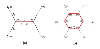
Figure 1: Schematic illustration of the (a) two- and (b) six-site cluster configurations. The lattice constant $a$ is set to unity, and the positions of three nearest neighbors of site A are $\delta_{1}=(1,0)$, $\delta_{2}=(-1/2,\sqrt{3}/2)$, $\delta_{3}=-(1/2,\sqrt{3}/2)$.

Moreover, the fermionic spinon Hamiltonian can be Fourier transformed into momentum space:

$$H^{f}_{\text{MF}} = \sum_{\bm{k},\sigma}\big{(}\varepsilon_{A\sigma}a_{\bm{k}\sigma}^{\dagger}a_{\bm{k}\sigma}+\varepsilon_{B\sigma}b_{\bm{k}\sigma}^{\dagger}b_{\bm{k}\sigma}$$ (10)

$$\hskip 20.00003pt+\Gamma_{\bm{k}}a_{\bm{k}\sigma}^{\dagger}b_{\bm{k}\sigma}+\Gamma_{\bm{k}}^{*}b_{\bm{k}\sigma}^{\dagger}a_{\bm{k}\sigma}\big{)}$$

with

$$\varepsilon_{A/B\sigma}=\tilde{\mu}_{A/B\sigma}-\mu-\lambda_{A/B\sigma}\;,$$

$$\Gamma_{\bm{k}}=-tZ\gamma_{\bm{k}}\;,\;\;\;\;\gamma_{\bm{k}}=\sum_{\bm{\delta}}e^{i\bm{k}\cdot\bm{\delta}}\;.$$ (11)

Diagnalization of the spinon Hamiltonian (10) gives rise to the eigenenergies as

$$E_{\bm{k}}^{\pm} = \pm\sqrt{|\Gamma_{\bm{k}}|^{2}+\Delta_{\sigma}^{2}}-\mu_{\text{eff}}\;,$$ (12a)

$$\mu_{\text{eff}} = \mu-\frac{1}{2}(\tilde{\mu}_{A\sigma}-\lambda_{A\sigma}+\tilde{\mu}_{B\sigma}-\lambda_{B\sigma})\;,$$ (12b)

$$\Delta_{\sigma} = \frac{1}{2}(\tilde{\mu}_{A\sigma}-\lambda_{A\sigma}-\tilde{\mu}_{B\sigma}+\lambda_{B\sigma})\;.$$ (12c)

Here, AFM energy gap $\Delta_{\text{AFM}}=|\Delta_{\sigma}|$ is identical in form to that in the square lattice caseLee and Lee (2017); Zeng et al. (2021).

In most occasions, it proves effective to adopt the density of states (DOS) of the non-interacting electrons to calculate the physical quantities in the thermodynamic limit. On the honeycomb lattice, it is defined as

$$D(\gamma) = \frac{1}{{\cal N}_{\text{triangle}}}\sum_{\bm{k}}\delta(\gamma-|\gamma_{\bm{k}}|)$$ (15)

$$= \Big{\{}\begin{array}[]{ll}N(\gamma)\;,&\;\;\;(0\leq\gamma<1)\\ \tilde{N}(\gamma)\;,&\;\;\;(1<\gamma\leq 3)\end{array}$$

where ${\cal N}_{\text{triangle}}$ is the site number of the underlying triangular lattice, which is half of that of the honeycomb lattice, and

$$\Bigg{\{}\begin{array}[]{l}N(\gamma)=\frac{4}{\pi^{2}}\frac{\gamma}{\sqrt{(3-\gamma)(1+\gamma)^{3}}}\,K\Big{(}\sqrt{\frac{16\gamma}{(3-\gamma)(1+\gamma)^{3}}}\,\Big{)}\;,\\ \tilde{N}(\gamma)=\frac{1}{\pi^{2}}\sqrt{\gamma}\,K\Big{(}\sqrt{\frac{(3-\gamma)(1+\gamma)^{3}}{16\gamma}}\,\Big{)}\;,\end{array}$$ (16)

with $K(x)$ being the first kind complete elliptical integral. In comparison to the self-dual situation on a square lattice, we now have a duality transformation

$$\tilde{\gamma}=\frac{3-\gamma}{1+\gamma}$$ (17)

to connect these two parts, under which

$$\frac{(3-\tilde{\gamma})(1+\tilde{\gamma})^{3}}{16\tilde{\gamma}} = \frac{16\gamma}{(3-\gamma)(1+\gamma)^{3}}\;,$$ (18a)

$$\frac{(3-\tilde{\gamma})(1+\tilde{\gamma})}{4\tilde{\gamma}} = \frac{4\gamma}{(3-\gamma)(1+\gamma)}\;,$$ (18b)

and

$$\tilde{N}(\gamma) = \frac{(3-\tilde{\gamma})(1+\tilde{\gamma})}{4\tilde{\gamma}}N(\tilde{\gamma})$$ (19)

$$= \frac{4\gamma}{(3-\gamma)(1+\gamma)}N\Big{(}\frac{3-\gamma}{1+\gamma}\Big{)}\;.$$

Then, the self-consistent quantities $\epsilon^{\delta}_{\sigma}=\epsilon$ and $n_{(A/B)\sigma}\equiv\langle a^{\dagger}_{i\sigma}a_{i\sigma}\rangle/\langle b^{\dagger}_{i\sigma}b_{i\sigma}\rangle$ can be calculated through

$$\!\!\!\!\!\!\!\!\epsilon=\int_{0}^{3}\!\!d\gamma\,D(\gamma)\frac{(tZ\gamma)^{2}}{6Z\sqrt{(tZ\gamma)^{2}+\Delta^{2}}}\sum_{s=\pm}s\theta[-E^{s}(\gamma)]\;,$$ (20)

$$\!\!\!\!\!\!\!\!n_{(A/B)\sigma}=\int_{0}^{3}\!\!d\gamma\,D(\gamma)\sum_{s=\pm}\theta[-E^{s}(\gamma)]$$

$$\hskip 40.00006pt\times\frac{1}{2}\Big{(}1\pm s\frac{\Delta_{\sigma}}{\sqrt{(tZ\gamma)^{2}+\Delta^{2}}}\Big{)}\;,$$ (21)

where $E^{\pm}(\gamma)=\pm\sqrt{(tZ\gamma)^{2}+\Delta^{2}}-\mu_{\text{eff}}$ and $\Delta_{\sigma}^{2}=\Delta^{2}$.

III RESULTS AND DISCUSSIONS

III.1 HALF-FILLED SYSTEM

In this case, the particle-hole symmetry implies $\mu^{\text{eff}}=0$ and $E^{+}(\gamma)>0$, and by relation (3), Eqs. (20) and (21) are simply

$$\epsilon = -\frac{t\lambda}{6}I_{\epsilon}(\lambda)\;,$$ (22)

$$\langle S_{(A/B)\sigma}^{z}\rangle = (-/+)\frac{\,{\rm sgn}({\Delta}_{\sigma})\,}{2}I_{S}(\lambda)\;,$$ (23)

where $\lambda=tZ/\Delta_{\text{AFM}}$ and

$$I_{\epsilon}(\lambda) = \int_{0}^{3}d\gamma\,D(\gamma)\frac{\gamma^{2}}{\sqrt{(\gamma\lambda)^{2}+1}}\;,$$ (24)

$$I_{S}(\lambda) = \int_{0}^{3}d\gamma\,D(\gamma)\frac{1}{\sqrt{(\gamma\lambda)^{2}+1}}\;.$$ (25)

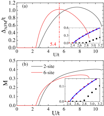
Figure 2: (a) The AFM energy gap $\Delta_{\text{AFM}}$ and (b) the staggered magnetization $M$ as function of $U$, where the insets show the same data in the vicinity of the critical coupling together with the fitting data (blue lines). The results from two-site cluster approximation are presented as well (black).

For the half-filled square lattice Hubbard model at $T=0$, the AFM order emerges for any nonzero $U$ because of the perfect nesting of the free Fermi surface, whereas the honeycomb lattice is known to have a semi-metal phase at small $U$ due to the low coordination number which allows more fluctuations and an antiferromagnetic phase at large $U$. It is well established that there is a single direct and continuous phase transition from semi-metal to AFMI at a finite critical interaction strength $U_{\text{AFM}}$ for the half-filled honeycomb lattice Hubbard model. This $U_{\text{AFM}}$ from large-scale QMC simulations mainly locates around $U\approx 3.8$ Sorella et al. (2012); Otsuka et al. (2016); Ostmeyer et al. (2021); Raczkowski et al. (2020); Assaad and Herbut (2013); Ma et al. (2018), whereas the results from various cluster scenarios, such as cluster dynamical impurity approximation, variational cluster approximation, dynamical cluster approximation and density matrix embedding theory, are strongly cluster dependent and the $U_{\text{AFM}}$’s are in a wide range of $1.5\lesssim U\lesssim 4.0$ Seki and Ohta (2012); Chen et al. (2014); Liebsch and Wu (2013b); Yamada (2016); Hassan and Sénéchal (2013). As shown in Fig. 2, we find that $U_{\text{AFM}}=2.75$ or 2.43 in our two- or six-site cluster approximation, which is larger than that from the Hartree-Fock approximation of 2.235 Sorella and Tosatti (1992); Raczkowski et al. (2020), but smaller than those from QMC simulations Otsuka et al. (2016); Assaad and Herbut (2013); Sorella et al. (2012); Ostmeyer et al. (2021); Ma et al. (2018), reflecting the fact that fluctuations have been incorporated in the six-site cluster, but not enough to give the accurate value. This shortcoming may be remedied by enlarging the cluster size and strictly dealing with the constraint $S^{z}_{\alpha}=f^{\dagger}_{\alpha}f_{\alpha}-\tfrac{1}{2}$ locally. However, the two-site cluster value of $U_{\text{AFM}}$ is larger than that from the six-site, necessitating more investigations on the dependence of $U_{\text{AFM}}$ upon the cluster size. To extract the critical information around $U_{\text{AFM}}$, we fit our self-consistent data from the six-site cluster using the $U$ dependent form of $M$ and $\Delta_{\text{AFM}}$ that have been verified by QMC simulations Otsuka et al. (2016); Assaad and Herbut (2013); Sorella et al. (2012); Ostmeyer et al. (2021) and density matrix embedding theory Chen et al. (2014)

$$\Delta_{\text{AFM}}/M=\alpha_{1/2}|U-U_{\text{AFM}}|^{\beta_{1/2}}\;,$$ (26)

and we obtain

$$\Big{\{}\begin{array}[]{ll}\alpha_{1}=0.74021\pm 0.00836\;,&\beta_{1}=0.77086\pm 0.01597\;;\\ \alpha_{2}=0.19739\pm 0.000753\;,&\beta_{2}=0.755\pm 0.0049\;.\end{array}$$ (27)

The critical exponent $\beta_{2}=0.755\pm 0.0049$ for $M$ is very close to $\beta_{2}=0.75\pm 0.06$ Otsuka et al. (2016) and 0.79 Assaad and Herbut (2013) from the large-scale QMC simulations, and $\beta_{2}=0.72$ from the density embedding theory Chen et al. (2014). It should be mentioned that $\beta_{2}=0.86546\pm 0.01849$ from the two-site approximation is close to that from the six-site one, and both results fall in the ballpark of the QMC estimates, reflecting the universal aspect of the critical exponent. The critical exponent for single particle gap $\Delta_{\text{AFM}}$ is slightly larger than that of $M$ Assaad and Herbut (2013); Ostmeyer et al. (2021).

We now expand asymptotically the integrals $I_{\epsilon}(\lambda)$ and $I_{S}(\lambda)$ defined in Eqs. (24) and (25) as $\lambda\to\infty$ Bleinstein and Handelsman (1986):

$$\epsilon=-\frac{t}{6}\Big{(}1.574597-0.448221\tilde{\Delta}^{2}+\frac{4}{3\sqrt{3}\pi}\tilde{\Delta}^{3}+\cdots\Big{)}\;,$$ (28)

$$\langle S_{(A/B)\sigma}^{z}\rangle = (-/+)\frac{\,{\rm sgn}({\Delta}_{\sigma})\,}{2}\Big{(}0.896441\tilde{\Delta}-\frac{2}{\sqrt{3}\pi}\tilde{\Delta}^{2}$$ (29)

$$-0.014\tilde{\Delta}^{3}+\frac{4}{9\sqrt{3}\pi}\tilde{\Delta}^{4}+\cdots\Big{)}\;,$$

where $\tilde{\Delta}=\lambda^{-1}=\Delta_{\text{AFM}}/tZ$. The relation between $M$ and $\Delta_{\text{AFM}}$ in the honeycomb lattice around $U=U_{\text{AFM}}$ is established as

$$M = \tfrac{1}{2}|\langle S_{A\sigma}^{z}\rangle-\langle S_{B\sigma}^{z}\rangle|$$

$$\approx \frac{1}{2}\Big{(}0.896441\tilde{\Delta}-\frac{2}{\sqrt{3}\pi}\tilde{\Delta}^{2}-0.014\tilde{\Delta}^{3}+\frac{4}{9\sqrt{3}\pi}\tilde{\Delta}^{4}\Big{)}\;.$$

To the leading order, $M\propto\Delta_{\text{AFM}}$, compared to $M\propto\Delta_{\text{AFM}}(\ln{\Delta_{\text{AFM}}})^{2}$ in the square lattice, supporting the AFM at small $U$ in the latter case is driven by the perfect nesting of its free Fermi surface.

On the other hand, $\Delta_{\text{AFM}}$ reaches its maximum around the crossover coupling strength $U_{c}=5.4t$ that separates the weak- and strong-coupling regimes, which is consistent with the traditional mean-field behavior $\Delta_{\text{AFM}}\sim U$ at small $U$, and $\Delta_{\text{AFM}}\sim 4t^{2}/U$ in the large $U$ limit supported by the super-exchange mechanism. It ought to be mentioned that $M$ drops abruptly when $U$ is larger than a certain value where the quasi-particle weight happens to drop to zero as shown in Fig. 3(a), implying that at half-filling, the cluster slave-spin method is incapable of capturing the crossover between the Hubbard model with finite $U$ and its counterpart in the large $U$ limit—the Heisenberg model, which can be understood from the expression of $M$ at half-filling

$$M=\frac{1}{2}|n_{A\sigma}-n_{B\sigma}|=\int_{0}^{3}d\gamma\,D(\gamma)\frac{|\Delta_{\sigma}|}{\sqrt{(tZ\gamma)^{2}+\Delta^{2}}}\;,$$ (31)

where the integration encounters $\frac{0}{0}$ when the AFM energy gap $\Delta_{\text{AFM}}$ and the quasi-particle residue $Z$ drop to zero simultaneously at large $U$ [See Fig. 2(a) and 3(a)]. However, for a doped system, $Z$ decreases to a constant [Fig. 4(a)] to be free from this glitch.

The quasi-particle residue $Z$, the generalized Gutzwiller factor $g_{t}$ Ogawa et al. (1975); Abram et al. (2013); Lee and Lee (2017), the holon-doublon correlators $C_{ij}$ Lee and Lee (2017) between the nearest neighbors $C_{12}$, the next-nearest neighbors $C_{13}$ and the next-next-nearest neighbors $C_{14}$, the ground state energy of the slave-spin Hamiltonian per site $\langle H_{n_{c}\text{-site}}^{S}\rangle/n_{c}$ with $n_{c}$ being the cluster size, and the double occupancy $\langle D\rangle$ as function of $U$ at half-filling obtained from two- and six-site cluster approximations are presented in Fig. 3, where $C_{ij}$ is defined as

$$C_{ij}=\frac{\langle N_{i}D_{j}\rangle-\langle N_{i}\rangle\langle D_{j}\rangle}{\langle N_{i}\rangle\langle D_{j}\rangle}\;,$$ (32)

with the holon operator $N_{i}=(1-n_{i\sigma})(1-n_{i\bar{\sigma}})$ and doublon operator $D_{j}=n_{j\sigma}n_{j\bar{\sigma}}$.

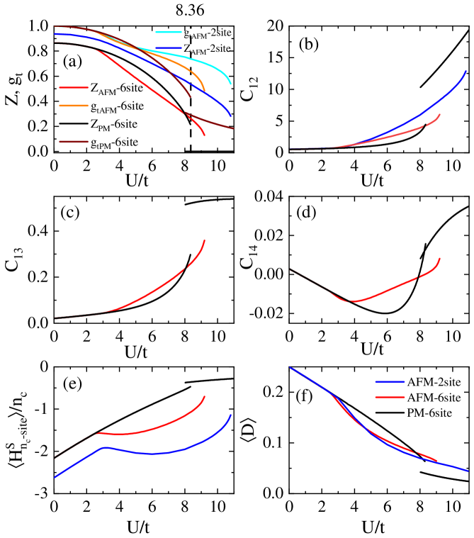
Figure 3: (a) The quasiparticle weight $Z$ and the generalized Gutzwiller factor $g_{t}$. (b)–(d) The holon-doublon correlators between the nearest neighbors $C_{12}$, the next-nearest neighbors $C_{13}$ and the next-next-nearest neighbors $C_{14}$. (e) The expectation value of the cluster slave-spin Hamiltonian $\langle H_{n_{c}\text{-site}}^{S}\rangle/n_{c}$. (f) The double occupancy $\langle D\rangle$ in the AFM state vs. $U$ obtained by the 2/6-site clusters (blue/red). All quantities in the PM state obtained by 6-site cluster are black lines.

The results are as follows: (i) All quantities in the PM state show discontinuities and hystereses at the critical coupling strength $U_{\text{Mott}}=8.36$ for the semi-metal to paramagnetic insulator transition as the characteristics of the first-order Mott transition in the PM state Hassan and Sénéchal (2013); Tran and Kuroki (2009). (ii) In Fig. 3(a), compared to that in the PM state, $Z$ is largely suppressed as entering the AFM phase. (iii) In Fig. 3(b)–(d), $C_{12}$ and $C_{13}$ are positive and increase monotonically with $U$, signaling that the holon and doublon between the nearest and next-nearest neighbors tend to attract each other, which is enhanced by the coupling strength. However, $C_{14}$ presents a negative minimum beyond the AFM transition or as $U$ approaches $U_{\text{Mott}}$ in the PM state, suggesting that at half-filling, the holon and doublon between the next-next-nearest neighbors attract each other when $U$ is small or large, while behave repulsively at intermediate $U$. (iv) In Fig. 3(e), $\langle H_{n_{c}\text{-site}}^{S}\rangle/n_{c}$ in the AFM state is smaller than that from the PM state, favoring an AFM ground state. (v) In Fig. 3(f), $\langle D\rangle$ in the PM state decreases linearly with the increasing $U$ when $U\ll U_{\text{Mott}}$ Vollhardt (1984), whereas in the AFM state, its slope changes abruptly as AFM sets in denoting a second-order transition from a semi-metal to an AFMI.

III.2 SYSTEMS WITH FINITE DOPING

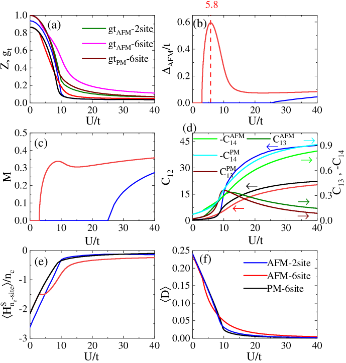
Figure 4: (a) The quasi-particle weight $Z$ and the generalized Gutzwiller factor $g_{t}$, (b) the AFM energy gap $\Delta_{\text{AFM}}/t$, (c) the staggered magnetization $M$, (d) the holon-doublon correlators between the nearest neighbors $C_{12}$, the next-nearest neighbors $C_{13}$ and the next-next-nearest neighbors $C_{14}$, (e) the expectation value of the cluster slave-spin Hamiltonian $\langle H_{n_{c}\text{-site}}^{S}\rangle/n_{c}$, and (f) the double occupancy $\langle D\rangle$ as function of $U$ at $\delta=0.02$ in the AFM state obtained by the two-site (blue) and six-site (red) cluster, as well as the PM state (black) by six-site cluster.

In Fig. 4, we plot $Z$, $g_{t}$, $\Delta_{\text{AFM}}$, $M$, $C_{12/3/4}$, $\langle H_{n_{c}\text{-site}}^{S}\rangle/n_{c}$, $\langle D\rangle$ as function of $U$ at $\delta=0.02$ obtained from two- and six-site cluster approximations to further compare the results from these two slave-spin clusters. In Fig. 4(a), the quasi-particle residue from six-site cluster is much smaller than that from two-site because of more quantum fluctuations, and becomes flattened when $U>U_{\text{Mott}}$. In Fig. 4(b), the critical coupling strength for AFM transition from six-site cluster is $U_{\text{AFM}}=3.0$, while that from two-site locates at $U_{\text{AFM}}=25.0$, which indicates that two-site cluster is inadequate to describe the AFM transition in the honeycomb lattice because it keeps no track of the lattice symmetry. In Fig. 4(d), $C_{12}$ increases slowly when $U<U_{\text{Mott}}$, then rises dramatically as $U$ approaches $U_{\text{Mott}}$, and finally grows progressively as $U$ goes to infinity; while $C_{13}$ shows a maximum near $U_{\text{Mott}}$, the reason for which is that the hopping probability between the next-nearest neighbors falls faster than the one between the nearest neighbors when $U$ is increased as demonstrated in our previous work on a square lattice Zeng et al. (2021). Unlike $C_{12}$ and $C_{13}$, both positive for all $U$’s, $C_{14}$ is negative at $\delta=0.02$ and its magnitude grows monotonically with the coupling strength, indicating that the holon and doublon between the next-next-nearest neighbors repulse each other, whose tendency is strengthened as $U$ increases. In Fig. 4(e), as shown by the blue line with $0<U<25$ (where the system within two-site approximation is in the PM state.) and the black line, the difference of $\langle H_{n_{c}\text{-site}}^{S}\rangle/n_{c}$ in PM state between two- and six-site cluster approximations is much smaller when $U>U_{\text{Mott}}$, denoting that the cluster size’s effect on the properties of the system in the PM state is less important at large $U$ as the system becomes more localized, where the inter-site fluctuations are much weaker in contrast to the weak-coupling limit. In Fig. 4(f), there exists an inflection in $\langle D\rangle$ in the PM state around $U\approx 10t$, meaning that the first-order Mott transition at half-filling turns into a continuous crossover at finite dopings. For $U<8.0$, the double occupancy in the AFM state is smaller than that in the PM state while the opposite is true for $U>8.0$, bespeaking that the AFM at small $U$ is triggered by the interaction potential gain while that in the large $U$ limit is not driven by this mechanism. This picture can also be seen in Fig. 5, where exists a region ($5.4<U<8.0$) with $\Delta E_{U}^{(S)}<0$ and $\Delta E_{K}^{(S)}<0$, signaling that the AFM in this region is supported by both the kinetic energy and interaction potential gain.

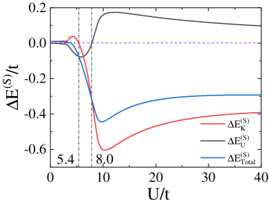
Figure 5: The difference of the kinetic energy $\Delta E_{K}^{(S)}$ (red), interaction potential $\Delta E_{U}^{(S)}$ (black), and their summation $\Delta E_{\text{Total}}^{(S)}$ (blue) of the six-site cluster slave-spin Hamiltonian Eq. (8d) between the AFM and PM states as function of $U$ at $\delta=0.02$.

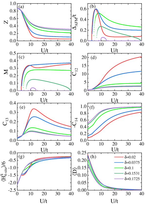
Figure 6: (a) The quasiparticle weight $Z$, (b) the AFM energy gap $\Delta_{\text{AFM}}/t$, (c) the staggered magnetization $M$, (d)–(f) the holon-doublon correlator between the nearest neighbors $C_{12}$, the next-nearest neighbors $C_{13}$ and the next-next-nearest neighbors $C_{14}$, (g) the expectation value of the cluster slave-spin Hamiltonian, and (h) the double occupancy $\langle D\rangle$ as function of $U$ at a series of doping concentrations $\delta=$ 0.02 (red), 0.0375 (blue), 0.1 (green), 0.1531 (dark green), 0.1725 (violet) in the AFM state obtained by the six-site cluster.

The dependence of the quantities discussed above upon the interaction strength at various dopings of $\delta=0.02,\,0.0375,\,0.1,\,0.1531,\,0.1725$ obtained through six-site cluster approximation are presented in Fig. 6, where $\delta=0.1531$ is the critical doping for the AFM to PM phase transition at $U=40$, and $\delta=0.1725$ is the maximum of $\delta_{M}$, i.e., the boundary between the AFM and PM state [see Figs. 8 and 11]. The following results are concluded: (i) In Fig. 6(a), the increasing $Z$ with $\delta$ for all coupling strengths suggests that the system with the increasing doping tends to be metallic. When $U>U_{\text{Mott}}$, the quasi-particle residues decrease progressively to constants, manifesting that the properties in the AFM state are controlled by the underlying Mott transition. (ii) In Fig. 6(b), $\Delta_{\text{AFM}}$’s at all dopings exhibit a maximum around the crossover coupling strength $U_{c}(\delta)$ that grows with $\delta$. (iii) In Fig. 6(d), $C_{12}$ increases monotonically with $U$ at all dopings and diminishes as $\delta$ goes up, which makes it eligible to be an indicator of the magnitude of correlations. (iv) In Fig. 6(g), compared to the PM state, $\langle H_{\text{6-site}}^{S}\rangle/6$ is suppressed dramatically as soon as AFM sets in and this effect is weakened by the increasing $\delta$.

The compressibility of the system is defined as $\kappa=n^{-2}\partial n/\partial\mu$. At $U=0$, it is calculated by using the non-interacting DOS $D(\gamma)$, Eq. (15), via

$$\kappa(\mu)=\Bigg{\{}\begin{array}[]{ll}\frac{N(|\mu|)}{[\frac{3}{4}+\int_{-1}^{\mu}N(|\gamma|)d\gamma]^{2}}\;,&\;\;(0<\delta<\frac{1}{4})\\ \frac{\tilde{N}(|\mu|)}{[\int_{-3}^{\mu}\tilde{N}(|\gamma|)d\gamma]^{2}}\;,&\;\;(\frac{1}{4}<\delta<1)\end{array}$$ (35)

which is proportional to the free DOS. For $U>0$, $\kappa$ should evolve simultaneously with the quasi-particle DOS which makes it adequate to indicate the dependence of this quantity upon interaction. The $\kappa$’s as function of $\delta$ at $U=0,\,2,\,4,\,6$, and 8 are plotted in Fig. 7. For $U<U_{\text{AFM}}$, the compressibility near the van Hove singularity is suppressed most drastically by interaction, while that at low energy (near the Dirac points) remains very close to the non-interacting one, reflecting that the Dirac cone structure is very robust, and the DOS of the quasi-particles is transferred away from the van Hove singularity as $U$ increases. Furthermore, at $U=4,\,6$, there exhibit a discontinuity at $\delta=\delta_{M}$ where the AFM-to-PM phase transition occurs, and the one-sided peak of $\kappa$ as $\delta$ approaches $\delta_{M}$ manifests that the system now is an itinerant AFM metal. However, at $U=8$, there exist two consecutive discontinuities: (i) between positively and negatively divergent $\kappa$; (ii) between negatively divergent and positive small $\kappa$.

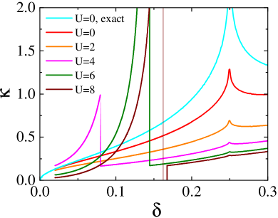
Figure 7: The compressibility $\kappa$ obtained from the six-site cluster approximation as function of $\delta$ at $U=0,\,2,\,4,\,6,\,8$ (red, orange, magenta, olive, brown, respectively), and the exact one at $U=0$ calculated through Eq. (35) (cyan).

IV PHASE DIAGRAM

The staggered magnetization $M$ with $U$ and $\delta$ being its parameters is plotted in Fig. 8, where the phase boundary between the AFM and PM states is delineated by $\delta_{M}(U)$. Obviously, $M$ maximizes at small dopings and large couplings. The phase boundary $\delta_{M}(U)$ shows a nonmonotonic behavior upon $U$ that may be connected to the crossover of $\Delta_{\text{AFM}}$ as $U$ increases. We also notice that $M$ saturates when $U>U_{\text{Mott}}$ at small dopings, reflecting that the physical properties in the AFM state are dominated by the underlying Mott transition in the half-filled PM state.

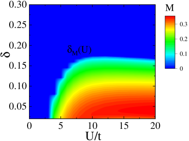
Figure 8: The staggered magnetization $M$ as function of $U$ and $\delta$ obtained by six-site cluster, where $\delta_{M}(U)$ is the phase boundary between the AFM and PM states.

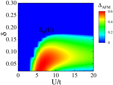
Figure 9: The AFM gap $\Delta_{\text{AFM}}$ as function of $U$ and $\delta$ obtained by six-site cluster with $\delta_{M}(U)$ separating the AFM and PM states.

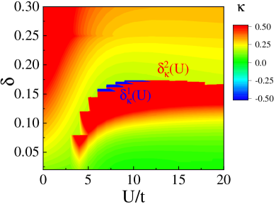
Figure 10: The compressibility $\kappa$ as function of $U$ and $\delta$ obtained by six-site cluster. The staircase is an artifact because of discrete $U$’s adopted to calculate $\kappa$, i.e., $\Delta U=t$ when $U\leq 10t$ and $\Delta U=2t$ when $10t<U\leq 20t$, which can only be eliminated in the $\Delta U\to 0$ limit. The blue region between $\delta_{\kappa}^{1}(U)$ and $\delta_{\kappa}^{2}(U)$ is characterized by $\kappa<0$, where $\delta_{\kappa}^{1}(U)$ and $\delta_{\kappa}^{2}(U)$ are delineated by the midpoints of the blue and red steps, respectively. The discontinuities in $\kappa$ at these two phase boundaries are reflected in the color jumpings.

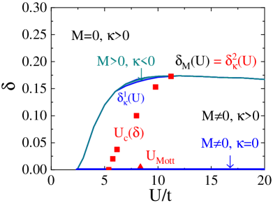
Figure 11: The $U$-$\delta$ phase diagram of the honeycomb lattice Hubbard model within the six-site cluster scheme. The critical coupling $U_{\text{Mott}}=8.36t$ for the Mott transition in the half-filled PM state is marked by the red triangle. The crossover coupling $U_{c}(\delta)$ in the AFM state at $\delta=$ 0, 0.02, 0.0375, 0.1, 0.1531 and 0.1725 are symbolled by red squares, at which $\Delta_{\text{AFM}}$ reaches its maximum. The half-filling case with $U>2.43t$ is highlighted by the heavy blue line, in which the system is an AFM insulator with $\kappa=0$.

The AFM energy gap $\Delta_{\text{AFM}}$ in the same parameter space is plotted in Fig. 9, where the phase boundary $\delta_{M}(U)$ still holds, denoting that there is no intermediate states before the semi-metal-to-AFMI transition occurs. An overall crossover between the weak- and strong-coupling regimes can be observed in $\Delta_{\text{AFM}}$ when $U$ grows, at which $\Delta_{\text{AFM}}$ reaches its maximum, and the coupling $U_{c}$ for this crossover is highly $\delta$-dependent, in contrast to that in the square lattice case Zeng et al. (2021). For $U>U_{c}$, the maximum of $\Delta_{\text{AFM}}$ occurs at $\delta\sim 0.075$, leading to an interesting vertical re-entrance behavior as $\delta$ increases, same as the square lattice case Zeng et al. (2021).

Combining Figs. 8, 9, and 10, an overall phase diagram in the $U$-$\delta$ plane emerges in Fig. 11. In contrast to the square lattice case Zeng et al. (2021), the crossover $U_{c}$ in the AFM state at which $\Delta_{\text{AFM}}$ is maximized, symbolled by the red squares, is shown to be highly $\delta$-dependent. On the other hand, $U_{c}$ at $\delta=0$ is smaller than $U_{\text{Mott}}$ (red triangle), implying that at half-filling, the coupling strength separating the weak- and strong-coupling regimes is suppressed by long-range AFM correlations Zeng et al. (2021). The blue region in this figure enclosed by $\delta^{1}_{\kappa}(U)$ and $\delta^{2}_{\kappa}(U)$ is characterized by $M\neq 0$ and $\kappa<0$ with $\delta^{1}_{\kappa}(U)$ being the phase boundary between $M\neq 0$, $\kappa>0$ and $M\neq 0$, $\kappa<0$, and $\delta^{2}_{\kappa}(U)$ between $M\neq 0$, $\kappa<0$ and $M=0$, $\kappa>0$. The region with $\kappa<0$ is extremely small compared to the square lattice Hubbard model Zeng et al. (2021), and exists only in the vicinity of the phase boundary between the AFM and PM state and at intermediate $U$. It should be noted that the phase diagram has been greatly improved from the two-site to six-site schemes, since in the former case $U_{\text{AFM}}$ jumps from $2.75t$ at $\delta=0$ to $25.5t$ at $\delta=0.02$, while in the latter it almost continuously from $2.43t$ to $2.97t$.

V CONCLUSION

We have exploited the cluster slave-spin method to explore extensively the ground state properties of the one-band honeycomb lattice Hubbard model with $U$ and $\delta$ as its parameters. At half-filling, the first-order semi-metal to insulator Mott transition in the PM state is revealed, characterized by discontinuities and hystereses in all quantities at $U_{\text{Mott}}=8.36t$ Hassan and Sénéchal (2013); Chen et al. (2014); Tran and Kuroki (2009). In the AFM state, a single direct and continuous phase transition between PM semi-metal and AFMI at $U_{\text{AFM}}=2.43t$ is substantiated, which belongs to the Gross-Neveu-Yukawa universality class Otsuka et al. (2016); Raczkowski et al. (2020); Assaad and Herbut (2013); Paiva et al. (2005); Yamada (2016); Sorella and Tosatti (1992); Sorella et al. (2012); Ostmeyer et al. (2020); Hassan and Sénéchal (2013), precluding the existence of intermediate phases such as a spin liquid state. At finite dopings, an extended crossover is discovered between the weak- and strong-coupling regimes in the AFM state at which the AFM energy gap $\Delta_{\text{AFM}}$ reaches its maximum, and the AFM within this crossover is driven by both the kinetic energy and interaction potential gain. The interaction $U_{c}$ for this crossover is shown to be highly $\delta$-dependent, in contrast to the square lattice system where $U_{c}$ remains almost unchanged with large dopings Zeng et al. (2021).

Moreover, for the half-filled system, by analytically calculating the relation between $M$ and $\Delta_{\text{AFM}}$ in the vicinity of PM semi-metal to AFM insulator transition, Eq. (III.1), we found that to the leading order, $M$ is linearly dependent on $\Delta_{\text{AFM}}$, compared to the square lattice result that is proportional to $\Delta_{\text{AFM}}(\ln{\Delta_{\text{AFM}}})^{2}$ (Ref. Zeng et al., 2021). This difference is consistent with the vanishing non-interacting DOS at Dirac points in the honeycomb lattice, in contrast to the van Hove singularity of the free electron DOS at the Fermi surface in a half-filled square lattice.

Finally, an overall phase diagram in the $U$-$\delta$ plane is presented in Fig. 11, the phase boundary $\delta_{M}(U)$ separating the AFM and PM phases shows a nonmonotonic behavior with the increasing $U$, which is consistent with the crossover behavior of $\Delta_{\text{AFM}}$. The phase boundary between the AFM metal with $\kappa>0$ and the AFM insulator with $\kappa=0$ locates exactly at $\delta=0$. The region with $\kappa<0$ only exists in the vicinity of the phase boundary between the AFM and PM state and at intermediate coupling strengths, whose area is extremely small compared to the counterpart in the square lattice Hubbard model Zeng et al. (2021).

It is worth mentioning that though lacking available data from the previous studies to verify our results at finite dopings, we corroborate that there is no intermediate states such as a spin liquid between the PM semi-metal and AFMI phases at half-filling Otsuka et al. (2016); Raczkowski et al. (2020); Assaad and Herbut (2013); Paiva et al. (2005); Yamada (2016); Sorella and Tosatti (1992); Sorella et al. (2012); Ostmeyer et al. (2020); Hassan and Sénéchal (2013), and the critical transition exponent of staggered magnetization between these two states is quite close to those from large-scale QMC simulations Sorella et al. (2012); Assaad and Herbut (2013); Otsuka et al. (2016); Ostmeyer et al. (2021) and DMET calculations Chen et al. (2014), which could well justify our calculations. We would like to mention that the interesting physics in the Hubbard model on a honeycomb lattice could be connected with the properties of graphen-based material Herbut (2006); Castro Neto et al. (2009); Ma et al. (2018, 2010); *PhysRevB.84.121410; *PhysRevB.90.245114, and also the optical lattice systems for ultracold atoms Messer et al. (2015). The ionic Hubbard model with ultracold fermions based on the honeycomb lattice has been realized where the transition from metal to charge density wave has been observed, and our theoretical prediction is consistent with the experimental results at the limit of stagger potential equal to zero. We hope our full phase diagram in the parameter space of on-site interaction and doping may simulate further experimental detection on graphene-based material or optical lattice systems for ultracold atoms.