Discovery of 40.5 ks Hard X-ray Pulse-Phase Modulations from SGR 1900+14 

Abstract

X-ray timing properties of the magnetar SGR 1900+14 were studied, using the data taken with Suzaku in 2009 and NuSTAR in 2016, for a time lapse of 114 ks and 242 ks, respectively. On both occasions, the object exhibited the characteristic two-component spectrum. The soft component, dominant in energies below $\sim 5$ keV, showed a regular pulsation, with a period of $P=5.21006$ s as determined with the Suzaku XIS, and $P=5.22669$ with NuSTAR. However, in $\gtrsim 6$ keV where the hard component dominates, the pulsation became detectable with the Suzaku HXD and NuSTAR, only after the data were corrected for periodic pulse-phase modulation, with a period of $T=40-44$ ks and an amplitude of $\approx 1$ s. Further correcting the two data sets for complex energy dependences in the phase-modulation parameters, the hard X-ray pulsation became fully detectable, in 12–50 keV with the HXD, and 6–60 keV with NuSTAR, using a common value of $T=40.5\pm 0.8$ ks. Thus, SGR 1900+14 becomes a third example, after 4U 0142+61 and 1E 1547$-$5408, to show the hard X-ray pulse-phase modulation, and a second case of energy dependences in the modulation parameters. The neutron star in this system is inferred to perform free precession, as it is axial deformed by $\approx P/T=1.3\times 10^{-4}$ presumably due to $\sim 10^{16}$ G toroidal magnetic fields. As a counter example, the Suzaku data of the binary pulsar 4U 1626$-$67 were analyzed, but no similar effect was found. These results altogether argue against the accretion scenario for magnetars.

1 INTRODUCTION

Through Suzaku and NuSTAR  observations in hard X-rays of the magnetars 4U 0142+61 (Makishima et al., 2014, 2019) and 1E 1547.0$-$5408  (Makishima et al. 2016; Makishima et al. 2021, hereafter Paper I), we have found a novel timing phenomenon; their hard X-ray pulses are phase-modulated with a long period of 55 ks and 36 ks, respectively. A likely origin of the effect (Makishima et al., 2014, 2016) is that the neutron stars (NSs) in these systems harbor toroidal magnetic fields $B_{\rm t}$ reaching $\sim 10^{16}$ G, and the magnetic pressure axially deforms the stars by $\epsilon\equiv\Delta I/I\sim 10^{-4}$ where $I$ is the moment of inertia. Then, the period $P_{\rm pr}$ of free-precession (= the pulse period) of the NS becomes slightly different from its rotation period $P_{\rm rot}$ around the symmetry axis, as $P_{\rm pr}=(1+\epsilon)P_{\rm rot}$. The beat between $P_{\rm pr}$ and $P_{\rm rot}$ appears at the so-called slip period given as

$$T=P_{\rm pr}/\epsilon\cos\alpha~{},$$ (1)

where $\alpha$ is the wobbling angle between the NS’s symmetry axis and the angular momentum vector ${\bf L}$, which are fixed to the NS and the inertial frame, respectively. We identify this $T$ with the observed pulse-phase-modulation periods. Further studies of this phenomenon will provide valuable information on $B_{\rm t}$ of magnetars, which are otherwise difficult to observationally estimate.

Of the two objects, 4U 0142+61 is an old magnetar with a characteristic age of $\tau_{\rm c}=65$ kyr, a pulse period of $P_{\rm pr}=8.69$ s, and a rather stable X-ray intensity. It represents a magnetar’s subclass called Anomalous X-ray Pulsars. In contrast, 1E 1547.0$-$5408  is a young object with $\tau_{\rm c}=0.7$ kyr and the fastest rotation ($P_{\rm pr}=2.07$ s) among the confirmed magnetars, exhibiting intensity changes by 4 orders of magnitude (Enoto et al., 2017). The detection of the hard X-ray pulse-phase modulation from these two contrasting magnetars suggests that it is a rather common phenomenon, to be detected possibly from almost all objects of this class.

Among the past observations, that of 1E 1547.0$-$5408  with NuSTAR  is of particular interest, because it allowed the discovery (Paper I) of peculiar energy dependences in the pulse-phase modulation parameters. Since this finding could provide valuable clues to the hard X-ray emission mechanism from magnetars, we need to analyze the data of other magnetars for similar phenomena. This makes a second aim of the present study.

Our study has yet another aim. The complex energy dependence in 1E 1547.0$-$5408  found with NuSTAR (Paper I) was not observed in the Suzaku data of the same object in an outburst (Makishima et al., 2016). Likewise, the modulation amplitude of 4U 0142+61 derived with NuSTAR  was much smaller than those measure with Suzaku  on two occasions (Makishima et al., 2019). Thus, the Suzaku and NuSTAR results, though generally consistent, are still subject to some differences, or possibly discrepancies. If these two X-ray observatories give more consistent results on some other magnetars, we will become more confident that we are not observing some instrument-specific artifacts.

The above three aims urge us to perform detailed hard X-ray timing studies of other magnetars. Obvious targets would be Soft Gamma Repeaters, namely, another major subclass of magnetars. In the present work, we hence select SGR 1900+14, a prototypical objects of this subclass. It has $P_{\rm pr}=5.2$ s and $\tau_{\rm c}=0.9$ ks, with an estimated distance of $12.5$ kpc (Davies et al., 2009), and exhibited a Giant Flare on 1998 August 27 (e.g., Feroci et al. 2001). Since it was observed by both Suzaku and NuSTAR, we utilize these archival data.

2 OBSERVATIONS

2.1 Suzaku

Throughout the 10 years of mission lifetime of Suzaku, SGR 1900+14 was observed twice. One was a Target-of-Opportunity observation (ObsID 401022010), from 2006 April 01 UT 08:42:57 for a gross pointing of 47 ks (Nakagawa et al., 2009; Enoto et al., 2010). The other (ObsID 404077010) was from 2009 April 26 UT18:23:44 for a gross pointing of 114 ks (Enoto et al., 2017). Since the former would be too short, we utilize the latter data set. It was already used by Enoto et al. (2017) in a summary study of the Suzaku observations of magnetars, but detailed timing studies have not yet been conducted at least to our knowledge.

In the 2009 observation, the X-ray Imaging Spectrometer (XIS) covering 0.5–10 keV (Koyama et al., 2007) was operated in the 1/4 window mode, with a time resolution of 2 s which is somehow usable for the study of the 5.2 s pulsation (see Makishima et al., 2014). From the three XIS cameras, XIS0, XIS1, and XIS3 that were operational at that time, we extracted events using an accumulation radius of $2^{\prime}$ around the source centroid. When the three cameras are added up, the source was detected with a count rate of $0.36$ ct s^-1 (background subtracted but vignetting uncorrected).

In the same observation, the Hard X-ray Detector (HXD; Takahashi et al. 2007; Kokubun et al. 2007) onboard Suzaku was operated in the standard mode. We utilize the data from HXD-PIN, with a nominal energy range of 10–70 keV, where the source was detected with a 12–50 keV rate of $0.046$ ct s^-1 after subtracting the modeled background (Enoto et al., 2017). The data from HXD-GSO are not utilized, because the source was not detected significantly.

The arrival times of the XIS and HXD data have been corrected for the barycentric motion of the Earth and the spacecraft.

2.2 NuSTAR

From 2016 October 20 UT 16:56:08, SGR1900+14 was observed with NuSTAR for an elapsed time of 242 ks (ObsID 30201013002). The archival data were already analyzed by Tamba et al. (2019), incorporating XMM-Newton data which were partially simultaneous. We do not utilize the XMM-Newton data set, because it covers only up to 10 keV with a short exposure (23 ks).

As described in Tamba et al. (2019), the NuSTAR data were processed using nupipeline and nuproducts in HEASoft 6.23, and the photon arrival times were corrected for the Earth and spacecraft motions around the Solar system barycenter. The net exposure was 122.6 ks after the standard pipeline processes. Since the nearby bright binary GRS 1915+105 caused severe stray light, particularly in FPMB, we utilize only the FPMA data, like in Tamba et al. (2019). To suppress the stray light, the on-source FPMA events were extracted from a circular region of $R_{\rm acc}=50^{\prime\prime}$ radius around the image centroid. The source was detected with a background-subtracted but vignetting-uncorrected count rate of $0.055$ ct s^-1 in 3–70 keV.

3 BASIC DATA ANALYSIS

3.1 Light curves

Figure 1 shows a 1–10 keV light curve of SGR 1900+14 obtained with the Suzaku XIS. The data, though suggesting some mild variations, are statistically consistent with being constant. We do not show light curves from the HXD, because they are background-dominated, and hence not informative. Similarly we skip showing the NuSTAR light curve, because it is already given in Fig. 5 of Tamba et al. (2019).

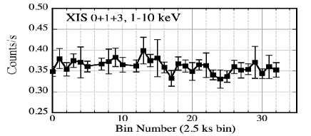
Figure 1: Light curve of SGR 1900+14 in 1–10 keV obtained with the Suzaku XIS (the 3 cameras added together), with 2.5 ks binning. The data include background (though negligible), and are not corrected for the vignetting. The data after bin 33 (82.5 ks) are omitted, because of rather frequent data gaps.

3.2 Spectra

Figure 2 presents the background-subtracted NuSTAR FPMA+FPMB spectrum of SGR 1900+14, and partly simultaneous XMM-Newton spectra, fitted jointly (Tamba et al., 2019) with a blackbody model for the Soft X-ray Component (SXC), and a power-law model for the Hard X-ray Component (HXC). The Suzaku spectrum, determined with the XIS and HXD (Enoto et al., 2017), is superposed as a best-fit incident model. As common among magnetars (Kuiper et al., 2006; Enoto et al., 2010), the spectra on the two occasions consist of the SXC and the HXC that cross over at $\sim 5$ keV. At the 12.5 kpc distance, the 1–60 keV luminosities measured with Suzaku and NuSTAR are $5.5\times 10^{35}$ erg s^-1 and $2.4\times 10^{35}$ erg s^-1, respectively. These are typical of this object, when it is not in an enhanced activity.

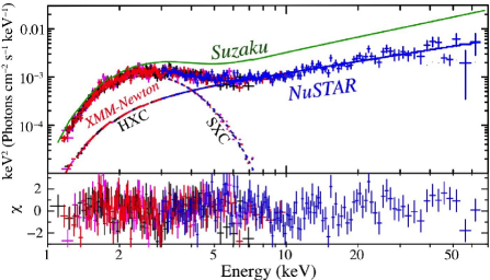
Figure 2: Background-subtracted NuSTAR  spectrum of SGR 1900+14 in blue. It is the same as Fig. 4 of Tamba et al. (2019), but converted to the $\nu F\nu$ form. Partially simultatneous XMM-Newton spectra are shown in red (PN), magenta (MOS1), and black (MOS2). The NuSTAR and XMM-Newton spectra are fitted jointly, by the sum of an absorbed blackbody for the SXC and a power-law for the HXC. The Suzaku spectrum (Enoto et al., 2017) is superposed as a green solid line, in the best-fit model form jointly determined with the XIS and HXD.

3.3 Periodograms

To study the pulsation expected at a period of $P\approx 5.2$ s, we utilize so-called $Z_{m}^{2}$ periodograms, wherein we epoch-fold the background-inclusive data into $N$ bins assuming a range of trial periods, and evaluate, at each $P$, the folded profile using $Z_{m}^{2}$ statistics (Brazier, 1994; Makishima et al., 2016, 2019). We do not correct each folded pulse profile for exposure, because it is very uniform (to within 2%) across the pulse cycle. The profiles hence preserve the photon counts.

The quantity $Z_{m}^{2}$ is obtained by summing up the Fourier power of the folded $N$-bin profile up to a specified maximum harmonic number $m$ ($\ll N$), and normalizing the result to the total event number (Paper I). The derived $Z_{m}^{2}$ is evaluated against $\chi^{2}$ distribution of $2m$ degrees of freedom (with a mean of $2m$ and 1$\sigma$ scatter by $\sqrt{4m}$), which $Z_{m}^{2}$ would follow if the data were dominated by Poisson noise. As $m$ is increased, $Z_{m}^{2}$ also gets larger, but becomes more noise dominated, because the pulse signal is usually limited to lower harmonics like $m\leq 5$. For $m\rightarrow N$, $Z_{m}^{2}$ approaches the usual chi-square of the pulse profile. Therefore, the $Z_{m}^{2}$ method with a small $m$ is more noise tolerant than the conventional chi-square technique, and unaffected by the choice of $N$ because $Z_{m}^{2}$ is independent of $N$ for $m\ll N$.

Figure 3 (a) shows a 1–10 keV pulse periodogram thus derived from the Suzaku XIS (the three cameras co-added). As a pilot study, we here employ $m=2$, considering that pulse profiles of some magnetars are double peaked. In spite of the limited XIS time resolution (2.0 s in this case), an outstanding peak with $Z_{2}^{2}=108$ has been revealed at a period of

$$P_{\rm XIS}=5.210\;06\pm 0.000\;15~{},$$ (2)

where we estimated the error conservatively as the half-width at half-maximum of the peak. The two side lobes seen at $P=5.205$ s and $P=5.215$ s are beat periods between $P_{\rm XIS}$ and the Suzaku’s orbital period, 5.6 ks. The three XIS cameras, when analyzed separately, gave consistent results, each with $Z_{2}^{2}$ from 26 to 42.

A hard X-ray periodogram from the same observation, derived with the 12–50 keV Suzaku HXD-PIN data, is presented in Fig. 3 (b). From the nominal energy range (10–70 keV) of HXD-PIN, those below 12 keV and above 50 keV were discarded, because of the dominance of thermal noise and particle background, respectively. The inset shows a detail near $P_{\rm XIS}$ of Equation (2). Although we observe several peaks with $Z_{2}^{2}$ exceeding $\sim 15$ up to $\sim 20$, none of them is dominating, and no enhancement is seen at $P_{\rm XIS}$, either.

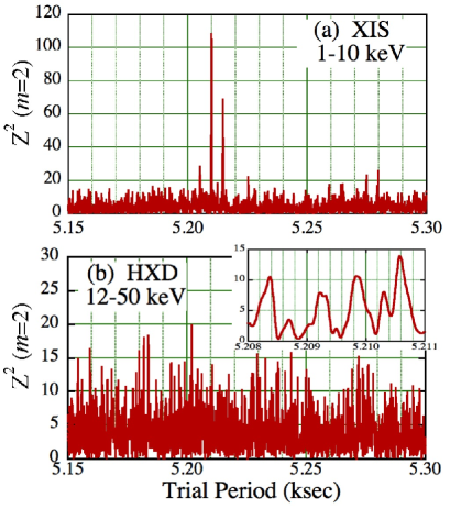
Figure 3: Pulse periodograms of SGR 1900+14 derived with Suzaku, using the $Z_{2}^{2}$ statistics. Panel (a) is from the XIS in 1–10 keV, whereas (b) is from the HXD in 12–50 keV. The inset to (b) gives a detail near $P_{\rm XIS}$.

Similarly, we analyzed the NuSTAR  FPMA data for the pulsation. Figure 4 shows periodograms derived in three typical energy bands. Panel (a), using the 3–70 keV range, reveals a clear peak reaching $Z_{2}^{2}=41.56$, at a period of

$$P_{\rm NuS}=5.226\;69\pm 0.000\;03~{},$$ (3)

which fully agrees with that reported in Tamba et al. (2019). For reference, the probability of finding a value of $Z_{2}^{2}\geq 41.56$ solely by chance is $2.1\times 10^{-8}$. It still gives a very low post-trial chance probability of $Q=2.8\times 10^{-5}$, after multiplied by 1330 which is the Fourier wave number (the effective number of frequency trials) contained in the period range of Fig. 3 and Fig. 4. We again observe two side lobes at $P=5.222$ s and $P=5.232$ s, arising from the beat with the NuSTAR’s orbital period, 5.8 ks. When the accumulation radius $R_{\rm acc}$ is varied from $38^{\prime\prime}$ to $100^{\prime\prime}$, the pulse significance became maximum for $R_{\rm acc}\approx 50^{\prime\prime}$ which we have employed.

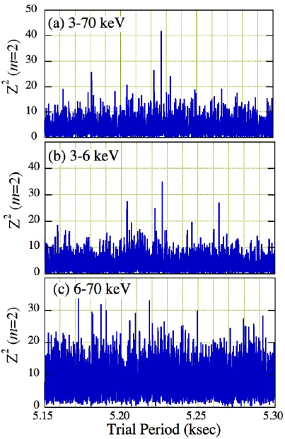
Figure 4: Same $Z_{2}^{2}$ periodograms as in Fig. 3, but derived with the NuSTAR FPMA in three energy ranges.

The periodogram peak at $P_{\rm NuS}$ is reconfirmed with $Z_{2}^{2}=34.82$ also in panel (b), which employs the 3–6 keV photons arising mainly from the SXC. However, the 6–70 keV periodogram in panel (c), representing the HXC, does not show any dominant peak, either at $P_{\rm NuS}$ or at any other period studied here. Even when different energy intervals above 6 keV were employed, the results did not change significantly.

In the SXC-dominant energies, thus the source pulsation has been detected significantly on the two occasions, and the derived periods are both consistent with the long-term spin-down history of the source after the Giant Flare in 1998; see Fig. 11 of Tamba et al. (2019). In contrast, neither data set gave evidence of pulsation in energies where the source signals are dominated by the HXC. These results remain unchanged even if using higher values of $m$. We present the folded pulse profiles of the SXC and HXC later in § 4.3.

4 DEMODULATION ANALYSIS

4.1 Demodulation formalism

The apparent absence of the HXC pulsation, both in the Suzaku and NuSTAR data, is reminiscent of the previous Suzaku results (§ 1) on 4U 0142+61 in 2009 (Makishima et al., 2014) and 1E 1547.0$-$5408 in the 2009 outburst (Makishima et al., 2016). In these cases, the hard X-ray ($\gtrsim 10$ keV) pulsations became detectable with high significance only after we correct, via so-called demodulation procedure, the photon arrival times for the pulse-phase modulation. The same correction also increased the HXC pulse significance in the NuSTAR data of 1E 1547.0$-$5408 in quiescence (Paper I). Supposing that the HXC pulses of SGR 1900+14 are in similar conditions, we apply the same timing corrections to the present two data sets.

The demodulation analysis assumes that the arrival times $t$ of individual pulses from the source are advancing/delaying periodically, by an amount

$$\delta t=A\sin(2\pi t/T-\psi)~{},$$ (4)

compared to the case of an exactly regular pulsation. Here, $T>0$, $A\geq 0$, and $\psi$ ($0\leq\psi<2\pi$) are the period, amplitude, and initial phase of the assumed modulation, respectively. Among them, $\psi$ can take any value between 0 and $2\pi$, as it simply reflects when the data acquisition happened to start. Then, by changing the arrival times of individual photons (instead of pulses) from $t$ to $t-\delta t$, we search for a set of parameters $(T,A,\psi)$ that maximize $Z_{\rm m}^{2}$ for the expected pulse period.

Although $T$ is unknown, a possible hint is provided by the inset to Fig. 3 (b). There, the periodogram shows several peaks separated in period by $\Delta P=(6-8)\times 10^{-4}$ s. Such structures could arise if the main periodicity is modulated in its amplitude or phase, at a long period of $P_{0}^{2}/\Delta P=(34-45)$ ks (Makishima et al., 2016), where $P_{0}$ stands for $P_{\rm XIS}$ or $P_{\rm NuS}$. Therefore, we set the search range of $T$ from 10 ks to 100 ks; at $T\lesssim 10$ ks, the analysis is often affected by the observatory’ s orbital period, and values of $T\gtrsim 100$ ks are not practical considering the overall data length (particularly of Suzaku).

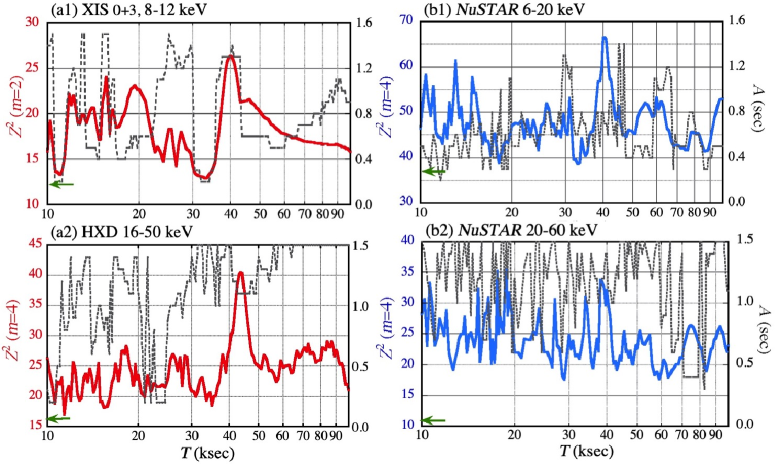
Figure 5: DeMDs derived from the Suzaku XIS (cameras 0+3) in 8–12 keV with $m=2$ (panel a1), the Suzaku HXD in 16–50 keV with $m=4$ (panel a2), and from the 6–20 and 20–60 keV NuSTAR data with $m=4$ (b1 and b2, respectively), all including background. The abscissa is $T$ in ks, and the red/blue curve (the left ordinate) gives the maximum $Z_{m}^{2}$ obtained at each $T$ when $A$, $\psi$, and $P$ are all varied. The dashed gray curve shows the value of $A$ (right ordinate) that maximizes $Z_{m}^{2}$. The green arrow at the bottom left of each panel indicates $Z_{m}^{2}$ before the demodulation, at $P\approx P_{\rm XIS}$ or $P\approx P_{\rm NuS}$.

4.2 Demodulation diagrams (DeMDs)

4.2.1 Suzaku XIS data

The demodulation analysis was first applied to the Suzaku XIS data, using the 8–12 keV range where the HXC dominates. Although the XIS energy response is poorly calibrated at $\gtrsim 10$ keV, we included the 10–12 keV interval because it still contains usable HXC signals, and the calibration uncertainties does not affect timing studies. We used the data from XIS0 and XIS3 (front-illuminated CCDs), but not those of the XIS1 camera (back-illuminated CCD chips), because its background at $\approx 10$ keV is more than an order of magnitude higher than those of the other two cameras (Koyama et al., 2007). The maximum harmonic number of $Z_{m}^{2}$ was tentatively set at $m=2$, because any Fourier component with $m\gtrsim 3$ of the pulse profile would be strongly smeared out by the XIS time resolution. As above, $T$ was varied over the 10–100 ks range, with a step of 0.2 s to 1.0 s (depending on $T$). At each $T$, we scanned $A$ from 0 s to 1.5 s with a step of 0.1 s, $\psi$ from $0^{\circ}$ to $360^{\circ}$ with a $5^{\circ}$ step, and $P$ over the error range of Equation (2) with a step of $20~{}\mu$s.

Figure 5 (a1) presents the maximum value of $Z_{2}^{2}$ achieved at each $T$, when $A$, $\psi$, and $P$ are all optimized. After Paper I, this kind of plot is hereafter called a demodulation diagram (DeMD). The result reveals a clear peak at

$$T=40.0^{+3.3}_{-2.5}~{}~{}{\rm ks}~{},$$ (5)

where the error is estimated as the range where $Z_{m}^{2}$ decreases by 4.72 from the peak value (Paper I). As shown in the same figure with a dashed gray curve, this peak has $A\approx 1.3$ s, or $\approx\pm 25\%$ of $P$. For reference, the XIS0 and XIS3 data, when analyzed separately, consistently reveal the 40 ks peak. When the XIS1 data are included, the peak becomes somewhat higher, but the DeMD becomes noisier in the $T=10-20$ ks interval, presumably due to the background variations.

As indicated by a green arrow in Fig. 5 (a1), the XIS data give $Z_{2}^{2}=12.29$ before the demodulation. Therefore, the 40 ks peak in the DeMD, with $Z_{2}^{2}=26.36$, yields $\delta Z_{2}^{2}=14.07$, where $\delta Z_{m}^{2}$ denotes a relative increment in $Z_{m}^{2}$, and provides a measure of the pulse-significance increase owing to the demodulation (Paper I). As a fiducial value, an increment by $\delta Z_{m}^{2}=10$ means a decrease in the probability $Q$ by a factor of $0.67\times 10^{-2}(1+\delta Z_{m}^{2}/Z_{m}^{2})^{m-1}$, or approximately by two orders of magnitude.

In Fig. 6 (a) we compare two periodograms, both computed using the 8–12 keV XIS 0+3 data. The black one is before the demodulation, whereas the red one is after the demodulation employing Equation (4) and $T=40.0$ ks, together with $A$ and $\psi$ as given in the figure. The result visualizes that the demodulation selectively enhances $Z_{2}^{2}$ at $P\approx P_{\rm XIS}$, although it is not necessarily obvious whether this peak is statistically significant.

4.2.2 Suzaku HXD data

To the background-inclusive HXD-PIN data, we applied the demodulation analysis with the same procedure as for the XIS, except that the search step in $\psi$ is reduced to $3^{\circ}$ and $m=4$ is employed. The latter is because the HXC pulse profiles of 4U 0142+61 and 1E 1547.0$-$5408, though variable, often exhibit three to four peaks per cycle when demodulated, and hence $m=4$ has generally been found most appropriate (Makishima et al. 2019; Paper I). In addition, we tentatively chose an energy range of 16–50 keV. The derived DeMD is presented in Fig. 5 (a2), where a prominent peak with $\delta Z_{4}^{2}=24.07$ is found at

$$T=43.5\pm 1.8~{}~{}{\rm ks}.$$ (6)

This $T$ is close to Equation (5), and the best-estimated amplitude of $A\approx 1.2$ s is consistent between the XIS and the HXD. The parameters characterizing this DeMD peak are summarized in Table 1 in comparison with those from the XIS.

The 16–50 keV HXD periodograms, before and after the demodulation, are shown in Fig. 6 (b) in black and red, respectively. The demodulation parameters employed in calculating the red periodogram are given in the figure. Thus, by correcting the data for the phase modulation with $T=43.5$ ks (Equation 6), the HXD pulses, which were undetectable in the raw data, have been clearly restored with $Z_{4}^{2}=40.64$, at a period of

$$P_{\rm HXD}=5.209\>88\pm 0.000\>03~{}{\rm s}.$$ (7)

The error is estimated in the same way as in Equation (5).

The HXD is a low-background but non-imaging instrument, and we are analyzing its data without subtracting the background which amounts to $\approx 91\%$ of the 16–50 keV events. Therefore, we must examine whether the pulse-phase modulation is an artifact caused by background variations. In the first 1/3 of the present observation, the spacecraft was in such orbits as to pass through the South Atlantic Anomaly, where the background is higher and more variable than in the rest (Kokubun et al., 2007). We hence divided the HXD data into three disjoint time portions with comparable durations, and applied the demodulation analysis to them individually, with the modulation period fixed at $T=43.5$ ks because it cannot be constrained. Then, the three portions gave $(A,\psi)$=(1.0 s, 213^∘), (1.4 s, 207^∘), and (1.1 s, 216^∘) in this order, together with $P$ which agrees with Equation (7). The parameters are thus similar among the three time portions, without correlation to the background behavior. Considering further the XIS vs. HXD similarities in $T$ and $A$, we conclude that the HXD results are not much affected by the background variations. We also infer that the 43.5 ks phase modulation of the HXD pulse is a coherent phenomenon, because the three portions, each covering about one modulation cycle, indicate consistent values of $\psi$.

As given in Appendix A, the chance probability $Q_{\rm HXD}$, for a value of $Z_{4}^{2}\geq 40.64$ to arise via statistical fluctuations, is estimated as $Q_{\rm HXD}\approx 4\%$. Since it is considered reasonably low, the phase modulation is likely to be real, rather than due to statistical fluctuations. The selection of $m=4$ is examined and justified in Appendix B.

For reference, we tried expanding the search range of $T$ up to 200 ks, considering the long data length (242 ks) of NuSTAR. However, no additional DeMD peaks were found.

4.2.3 Puzzles with the Suzaku data

As seen so far, the XIS and HXD data suggest that the HXC pulses of SGR 1900+14 on this occasion were phase-modulated with $T=40-44$ ks and $A\approx 1.2$ s. However, several inconsistencies and puzzles still remain within the HXD data, and between the XIS and HXD data. They are;

1. When the lower energy bound of the HXD data is lowered from 16 keV, the $T\approx 43.5$ ks DeMD peak gradually diminishes, down to $Z_{4}^{2}=33.09$ in 12–50 keV.

2. The $T=43.5$ ks peak of the 16–50 keV HXD data is accompanied by $\psi=216^{\circ}$ (Table 1), but it changes to $\psi\approx 60^{\circ}$ if using, e.g., the 12–18 keV band instead. The latter is not consistent, either, with that from the XIS ($\psi\approx 160^{\circ}$).

3. The values of $T\approx 40.0$ ks indicated by the XIS (Equation 5) and $T\approx 43.5$ ks by the HXD (Equation 6) appear somewhat discrepant.

4. As in Fig. 6 (b), the optimum pulse period from the demodulated HXD data falls on the lowest end of the conservatively estimated error range of $P_{\rm XIS}$.

Among the above issues, [S1] must be taken most seriously, because it is specific to the HXD data, and hence is free from the limited XIS time resolution. It is on one hand consistent with the pulse non-detection (using $m=2$) in Fig. 3 (b). On the other hand, it is puzzling, because expanding the energy range from 16–50 keV to 12–50 keV should normally increase $Z_{4}^{2}$ (see an argument in the next subsection). Therefore, we infer that the pulse coherence degrades when a broader energy range is used, as seen in Paper I. We return to this issue after analyzing the NuSTAR data.

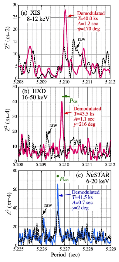
Figure 6: Detailed pulse periodograms. (a) The Suzaku XIS result in 8–12 keV, where the dashed black curve denoted “raw” uses the background-inclusive XIS photons without timing corrections, whereas red is that after applying the demodulation via Equation (4) assuming $T=40.0$ ks. The employed $A$ and $\psi$ are given in the figure. (b) The HXD result in 16–50 keV, where the meanings of the curves are the same as in panel (a). The red trace employs $T=43.5$ ks. The horizontal green bar represents $P_{\rm XIS}$ (with the associated errors). (c) Te 6–20 eV NuSTAR result, before (black) and after (blue) the demodulation with $T=40.5$ ks.

4.2.4 NuSTAR data

We applied the same demodulation analysis to the NuSTAR data, and obtained the DeMDs in panels (b1) and (b2) of Fig. 5, together with the periodograms in Fig. 6 (c). The lower energy bound of 6.0 keV is chosen to approximately coincide with the SXC vs. HXC cross-over energy (Tamba et al., 2019), and is made somewhat lower than that for the XIS (8 keV), because the NuSTAR effective area at these energies decreases towards lower energies, whereas that of the XIS behaves in the opposite sense. The 6.0–20 keV DeMD reveals a strong peak with $Z_{4}^{2}=66.51$ ($\delta Z_{4}^{2}=29.35$) at

$$T=40.5\pm 0.8~{}~{}{\rm ks}~{}.$$ (8)

The error is about half that in Equation (6), reflecting the NuSTAR data length which is about twice longer than that with Suzaku. The corresponding DeMD peak is also recognized in the 20–60 keV result at a consistent $T$, although it is considerably less conspicuous, and the amplitude, $A\approx 1.2$ s, is somewhat larger than that in 6–20 keV, $A\approx 0.7$ s.

The reality of the above results was examined in several ways. First, like in the HXD case, we applied the same analysis to the 1st and 2nd halves of the 6–20 keV NuSTAR data, this time allowing $T$ also to vary. Then, the two halves yielded fully consistent DeMDs, in terms of $T$, $A$, and $\psi$. Next, like in § 3.3, we changed $R_{\rm acc}$, to find that the DeMD peak again becomes highest at $R_{\rm acc}\approx 50^{\prime\prime}$, while the modulation parameters ($T$, $A$, and $\psi$) depend little on $R_{\rm acc}$, at least from $35^{\prime\prime}$ to $100^{\prime\prime}$. Therefore, the result is not likely an artifact caused by the stray light from GRS 1919+105. Finally, as given in Appendix A, the peak with $Z_{4}^{2}=66.51$ has a post-trial chance probability of $Q_{\rm NuS}\approx 1\%$, which is even lower than $Q_{\rm HXD}$. We hence conclude that the phase modulation in the 6–20 keV NuSTAR data is real.

4.2.5 Puzzles with the NuSTAR data

From these DeMDs, we presume that the Suzaku and NuSTAR data recorded the same phenomenon. The value of $T$ indicated by NuSTAR is in fact consistent with that of the XIS ($\approx 40.0$ ks; Equation 5), However, $T$ could be inconsistent between the HXD ($\approx 43.5$ ks; Equation 6) and NuSTAR ($\approx 40.5$ ks). If so, the problem [S3] in § 4.2.3 is unlikely to be an artifact due to the limited time resolution of the XIS, and must be regarded as inherent to the HXD data.

Even ignoring for the moment this HXD vs. XIS (plus NuSTAR) discrepancy in $T$, the NuSTAR data themselves are subject to the following two puzzles.

1. When the two NuSTAR energy ranges used in Fig. 5, 6–20 and 20–60 keV, are added together, the 40 ks DeMD peak decreases to $Z_{4}^{2}=44.97$, which is higher than that in 20–60 keV (33.47) but much lower than in 6–20 keV (66.51).

2. As in Table 1, we find $\psi=3^{\circ}$ and $\psi=246^{\circ}$, in 6–20 and 20–60 keV, respectively. The latter, calculated for $T=38.7$ ks, becomes $\psi\approx 160^{\circ}$ if using $T=40.5$ ks. Therefore, the initial phase is $\sim 180^{\circ}$ off between the two energy ranges.

Evidently, [N1] and [N2] are of the same nature as [S1] and [S2], respectively. In particular, [N1] (as well as [S1]) is puzzling, because periodic signals with a constant pulse profile and insignificant background should satisfy a relation as (Paper I)

$$Z_{m}^{2}\propto N_{\rm tot}\times({\rm PF})^{2}$$ (9)

where $N_{\rm tot}$ is the total number of signal photons, and PF is the pulsed fraction.

4.3 Pulse profiles

The issues [S1] and [N1] suggest that the pulse profiles and/or phases are considerably energy dependent, so the PF degrades when the energy range is expanded. To examine this possibility, let us look at the folded pulse profiles in various energies from the two data sets.

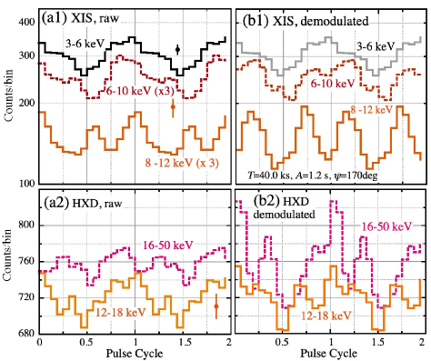
Figure 7: Background-inclusive pulse profiles of SGR 1900+14 obtained with Suzaku, shown for two cycles after applying the running average (see ext). The ordinate is in units of counts per bin. (a1) Three-band XIS pulse profiles, folded at $P_{\rm XIS}$ of Equation (2). The ordinate is logarithmic, and the 6–10 keV and 8–12 keV profiles are both multiplied by a factor of 3. (a2) Results from the HXD in two energy intervals, folded also at $P_{\rm XIS}$. The ordinate is linear, because the data are background dominated. (b1) The same as (a1), but the 6–10 keV and 8-12 keV results have been demodulated, using $T=40.0$ ks, $A=1.2$ s, $\psi=160^{\circ}$, and $P=P_{\rm XIS}$. (b2) The HXD profiles in the same energy bands as in (a2), but demodulated using $T=43.5$ ks, $A=1.1$ s, $\psi=225^{\circ}$, and $P=5.20987$ s.

Figure 7 shows background-inclusive pulse profiles with the Suzaku XIS (panel a1) and the HXD (panel a2), folded under the conditions as specified in caption. Here and hereafter, we include the XIS1 data, because its background is stable on time scales of seconds. The profile is always shown after taking a running average, where we smooth a time series $\{x_{j}\}$ by replacing $x_{j}$ with $0.25x_{j-1}+0.5x_{j}+0.25x_{j+1}$. This reduces the statistical fluctuation in each data bin to 0.61 times the original Poisson value (Paper I). The derived profiles are single-peaked at $\lesssim 10$ keV, and changes into a double-peaked shape in $\gtrsim 10$ keV. However, the profiles appear rather different between the 8–12 keV XIS data and the 12–18 keV HXD data.

Through demodulation using the parameters given in the caption, the profiles changed into as in panels (b1) and (b2). The 6–10 and 8–12 keV profiles became double-peaked, and that in 16–50 keV changed drastically; the PF increased, and several sharp features emerged. However, the 12–18 keV HXD profile is still different from the 8–12 keV XIS result. In addition, the deep pulse minimum appears to move, in complex ways, across the whole XIS plus HXD energy range. These results support our view that the issue [S1] stems from energy-dependent pulse-profile changes that cannot be rectified by the demodulation.

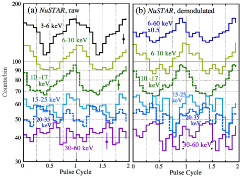
Figure 8: Same as Fig. 7, but obtained with NuSTAR. The ordinate is logarithmic. (a) Pulse profiles in slightly-overlapping six energy intervals, all folded at $P_{\rm NuS}$. (b) The same as panel (a), but the profiles above 6 keV have all been demodulated, assuming $T=40.5$ ks, $A=0.7$ s, $\psi=3^{\circ}$, and $P_{\rm NuS}$, referring to Table 1. The 3–6 keV profile in (a) is replaced with the demodulated 6–60 keV one (blue), which is halved for presentation.

The background-inclusive NuSTAR pulse profiles are given in Fig. 8 (a), again incorporating the running average. Like in the Suzaku case, the profiles are single-peaked up to the 10–17 keV range, and become double- (or multiple-) peaked in 15–25 keV and beyond. In panel (b), we applied the demodulation to the profiles except in the lowest 3–6 keV range, using a common set of parameters determined in 6–20 keV (Table 1). The pulse amplitude increased mainly in $>15$ keV. However, the pulse-phase assignment still remains ambiguous between energies above and below $\sim 15$ keV. In relation to the problem [N1], this suggests considerable changes in the pulse properties across $\sim 15$ keV. Furthermore, in both panels the pulse phase appears to advance from the 6–10 keV to 10–17 keV intervals.

With both Suzaku and NuSTAR, we have thus confirmed that the demodulation actually increases the pulse significance, and hence the PF from Equation (9), at least in some energy intervals. However, the pulse profiles still depend on the energy in rather complex ways in both data sets; presumably, this is responsible for [S1] and [N1], and possibly for [S2] and [N2] as well. In addition, we have come across yet another issue that is common to the two data sets:

• The pulse-peak phase shifts gradually as a function of energy, although the sign of this shift is not necessarily clear.

Table 1: A summary of the demodulation analysis, with 1-sigma errors.

Energy (keV)	Conditiona	$P$	$Z_{4}^{2}$	${\delta Z_{4}^{2}}^{\,b}$	$T$	$A^{\rm c}$	$\psi^{\,\rm d}$
and $m$		(sec)			(ks)	(sec)	(deg)
Suzaku
8–12 (XIS 0+3)	Raw	$5.21000(15)$	12.29	—	—	—	—
($m=2$)	Simple Dem.	$5.21004(12)$	26.36	14.07	$40.0^{+3.3}_{-2.5}$	1.3	160
16–50 (HXD)	Raw	5.20999${}^{c}~{}~{}~{}~{}$	16.57	—	—	—	—
($m=4$)	Simple Dem.	5.20987(3)	40.64	24.07	$43.5\pm 1.8$	1.1	216
12–50 (HXD)	Raw	5.20984${}^{e}~{}~{}~{}~{}$	17.21	—	—	—	—
($m=4$)	Simple Dem.	5.20990(3)	33.09	15.88	$43.7\pm 2.6$	1.2	225
	EDPV1	5.21002 (3)	41.57	24.36	$41.9\pm 1.8$	1.1	153
	EDPV2	5.21003 (3)	47.98	30.77	$41.2\pm 1.2$	1.1	159
NuSTAR
6–20	Raw	5.22669 (2)	37.16	—	—	—	—
$(m=4)$	Simple Dem.	5.22671 (2)	66.51	29.35	$40.5\pm 0.8$	0.7	3
20–60	Raw	5.22669 (2)	10.65	—	—	—	—
$(m=4)$	Simple Dem.	5.22671 (2)	33.47	22.82	$38.7^{+2.2}_{-1.0}$	1.2	246
6–60	Raw	5.22672 (2)	23.11	—	—	—	—
$(m=4)$	Simple Dem.	5.22670 (2)	44.97	21.86	$40.6\pm 1.1$	0.7	0
	EDPV1	5.22670 (2)	59.04	35.93	$40.5\pm 0.7$	0.9	0
	EDPV2	5.22670 (2)	64.70	41.59	$40.6\pm 0.5$	1.0	6

• : “Raw”= without timing correction, “Simple Dem.”=with energy-independent demodulation via Equation (4), “EDPV1”=using Equation (11), and “EDPV2”=incorporating equations (11) and (12).

• : Increment in $Z_{4}^{2}$ from the “Raw” value.

• : The errors associated with $A$ are typically $\pm 0.3$ for Suzaku and $\pm 0.2$ for NuSTAR.

• : The errors associated with $\psi$ are typically $\pm 30^{\circ}$ for Suzaku and $\pm 15^{\circ}$ for NuSTAR, reflecting the overall data length.

• : The error is not estimated because the peak is not outstanding.

4.4 Analysis of the soft-component signals

To examine whether the SXC signals also suffer the pulse-phase modulation, we applied the same analysis to the 1–5 keV XIS data (combining the three cameras) with $m=2$, and the 3–5 keV NuSTAR data with $m=4$. The upper energy bound, 5 keV, was selected to exclude the HXC, and the choice of $m$ is the same as before. The inclusion of the XIS1 data is because its background is negligible at these energies.

The derived soft-band DeMDs are presented in Fig. 9. Although a broad enhancement is seen in the XIS DeMD (panel a) over a range of $T=40-45$ ks, the increment is only $\delta Z_{2}^{2}\sim 4$, and the associated amplitude, $A\sim 0.2$ s, is only $\sim 4\%$ of $P$. We do not find particular $Z_{4}^{2}$ enhancements at $T\sim 40$ ks of the NuSTAR DeMD (panel b), either, even though the allowed values of $A$ are relatively large, $A\lesssim 0.8$ s, due to the small photon number (1658 events) in this energy band. More generally, around the mean of $\langle Z_{4}^{2}\rangle=41.98$ in the NuSTAR DeMD, $Z_{4}^{2}$ is seen to fluctuate by $\pm 3.63$ (1$\sigma$), in agreement with the expectation of $\sqrt{4m}=4.0$.

We hence conclude that the SXC pulsation is free from the phase modulation that affects the HXC pulses. This agrees with the results on the preceding two magnetars (Makishima et al. 2016, 2019; Paper I), and indicates a basic difference between the two spectral components in their timing properties.

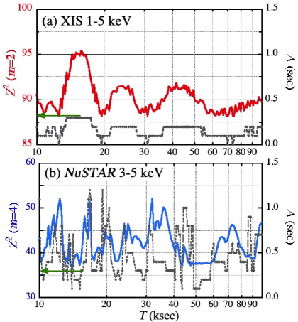
Figure 9: Soft-band DeMDs, obtained with the Suzaku XIS in 1–5 keV using $m=2$ (panel a), and with NuSTAR in 3–5 keV using $m=4$ (panel b). The meanings of red/blue and dashed gray traces are the same as in Fig. 5.

5 ADVANCED TIMING STUDIES

Although the demodulation analysis was partially successful, we are still left with the problems: [S1] –[S4] (§ 4.2.3), [N1], [N2](§ 4.2.5), and [SN1] (§ 4.3). We suppose that these issues at least partially arise via energy dependences in the pulse-phase-modulation phenomenon (Paper I). By empirically modeling these effects, we hope to solve or explain the issues, in terms of the basic dynamics of an axial rigid body, i.e., rotation around the symmetry axis and free precession.

5.1 Preliminary evaluations

A possibility suggested by [S1], [S2], [N1], and [N2] is that $\psi$ in Equation (4) depends on the energy, changing considerably across a narrow interval around 15 keV. Actually, such an effect was observed from 1E 1547.0$-$5408 (Paper I); as the energy increases from 10 keV to 27 keV, $\psi$ decreased by $\sim 65^{\circ}$, followed by a $180^{\circ}$ jump.

To examine the above possibility, we conducted a few preliminary tests. Figure 10 (a1) and (a2) show so-called double-folded maps using the Suzaku HXD data. The abscissa is the pulse phase $\Phi/2\pi$, the ordinate (from top to bottom) the modulation phase $\Psi/2\pi$, and the colors represent the photon intensity. The value of $\Psi$ at the observation start is $\psi$ in Equation (4). As in Paper I, the running average is applied in the $\Phi$ dimension, but not in $\Psi$. The correction for exposure is applied only in $\Psi$, because it is highly uniform in $\Phi$. In both panels, the pulse peak forms a yellow vertical ridge at $\Phi/2\pi\approx 1.0$, but it wiggles as a function of $\Psi$, just visualizing the pulse-phase modulation. The lateral swing of the ridge in (a2), $\approx\pm 0.2P$, agrees with the observed $A\approx 1.0$ s. Moreover, the wiggles in the two panels occur in the opposite sense; in (a1), it is most delayed in $\Phi$ at $\Psi/2\pi\approx 0.3$ and most advanced at $\Psi/2\pi\approx 0.7$, but in (a2) the largest delay and advance occur at $\Psi/2\pi\approx 0.9$ and $\approx 0.4$, respectively. This confirms that $\psi$ changes by $\approx 180^{\circ}$ between the two energy bands.

Using the NuSTAR  data, we conducted a more quantitative evaluation, to obtain the results in Fig. 10 (b). In several energy bands (with partial overlaps), we calculated $Z_{4}^{2}$ as a function of $\psi$, keeping $T=40.5$ ks but allowing $P$ and $A$ to vary. In the 6–12 keV band, $Z_{4}^{2}$ became highest at $\psi\sim 0^{\circ}$, but toward higher energies this peak increased in $\psi$, and reached $\psi\approx 160^{\circ}$ at the 20–60 keV range. This is consistent with the implications from Suzaku, and supports our conjecture, although $\psi$ increases towards higher energies contrary to the behavior of 1E 1547.0$-$5408.

In the NuSTAR observation of 1E 1547.0$-$5408  in 2016, not only $\psi$ but also $A$ exhibited strong energy dependences, with a factor $\sim 3$ enhancement at $22\pm 7$ keV (Paper I). In the present case, such behavior is not observed, because we always find $A\approx 1.0$ s within $\pm 30\%$ (Table 1). We hence treat $A$ as an energy-independent constant, although we do not require it to be the same between the two observations.

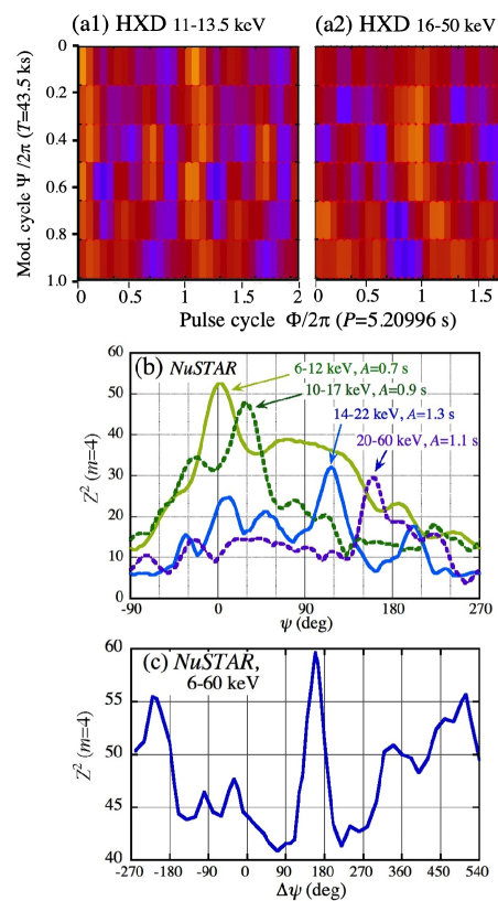
Figure 10: (a1) Double-folded map (see text) produced from the 11.0–13.5 keV HXD data using $P$ of Equation (7) and $T=43.5$ ks of Equation (6), where the photon intensity is represented by the color gradient (yellow, red, and blue from brightest to faintest). (a2) Same as (a1), but using the 16.0–50.0 keV HXD data. (b) Maximum values of $Z_{4}^{2}$ in four energy intervals of the NuSTAR data, shown as a function of $\psi$. (c) The highest $Z_{4}^{2}$ from the 6–60 keV NuSTAR data, derived via the EDPV1 correction, shown as a function of $\Delta\psi$. Except $T=40.5$ ks, all the parameters are free.

5.2 Formalism

Following Paper I, we modify Equation (4), and empirically model the HXC pulse timing behavior as

$$\delta t=P\cdot S(E)/360+A\sin\left[2\pi t/T-\psi(E)\right]~{},$$ (10)

which we call Energy Dependent Pulse-phase Variation (EDPV). Here, $E$ is the energy in units of keV, and $\psi(E)$, in place of the constant $\psi$ in Equation (4), describes how the modulation phase varies with $E$. The other variable $S(E)$ describes, in units of degree (0 to $360^{\circ}$), the energy dependence of the pulse phase [SN1]. On a double-folded map like Fig. 10 (a1,a2), $\psi(E)$ and $S(E)$ specify vertical ($\Psi$ direction) and horizontal ($\Phi$ direction) displacements of the pulse pattern, respectively, both as functions of $E$. While $\psi(E)$ is coupled with the pulse-phase modulation at $T$, $S(E)$ is not.

Based on the preliminary evaluations, as well as Paper I, let us model $\psi(E)$ as

$$\psi(E)=\left\{\begin{array}[]{ll}\psi_{0}&(E\leq E_{1})\\ \psi_{0}+\Delta\psi\;(E-E_{1})/(E_{2}-E_{1})&(E_{1}<E<E_{2})\\ \psi_{\rm 0}+\Delta\psi&(E_{2}<E)\end{array}\right.$$ (11)

where $E_{1}$, $E_{2}$, and $\Delta\psi$ are adjustable parameters, and $\psi_{0}$ gives the initial modulation phase at $E\leq E_{1}$. Thus, $\psi(E)$ remains at $\psi_{0}$ for $E\leq E_{1}$, changes linearly by $\Delta\psi$ from $E_{1}$ to $E2$, and stays at $\psi_{0}+\Delta\psi$ for $E\geq E_{2}$. (Compared to Paper I, $\Delta\Psi$ is here defined using the opposite sign, to make the present results easier to grasp.) This modeling is hereafter referred to as EDPV1.

We model $S(E)$ in a parabolic way as (Paper I)

$$S(E)=\left\{\begin{array}[]{ll}0&(E\leq 8~{}{\rm keV})\\ \frac{R}{(E_{3}-8)}(E-8)(E_{3}-E)&(E>8~{}{\rm keV})~{},\\ \end{array}\right.$$ (12)

using two parameters $R$ and $E_{3}$. Thus, $S(E)$ is assumed to work in $E>8$ keV (see § 5.3.2), with a slope $R\equiv(dS/dE)_{\rm 8keV}$ at 8 keV in units of deg keV^-1. If $R>0$, $S(E)$ increases up to $E=(8+E_{3})/2$ keV where it reaches $R\,(E_{3}-8)/4$, then it starts decreasing, returns to 0 at $E_{3}$, and becomes negative for $E>E_{3}$. If $R<0$, $S(E)$ behaves in the opposite way. The timing correction by Equation (12), together with Equation (11), is hereafter called EDPV2 modeling.

Below, we focus on the HXD and NuSTAR  data in the 12–50 keV and 6–60 keV bands, respectively, which are nearly the widest ranges where the HXC is clearly detected. The EDPV1 scheme is first applied to the data, to confirm its effectiveness, and to optimize its parameters ($\Delta\psi$, $E_{1}$, and $E_{2}$), separately for the two data sets. Then, we proceed to the EDPV2 corrections. These attempts are not performed on the XIS data.

Table 2: Summary of the optimum EDPV parameters, with 1-sigma errors.

Function	$\psi(E)$					$S(E)$
Parameer	$\Delta\psi$	$\psi_{0}^{\,a,b}$	$E_{1}$	$E_{2}$		$R$	$E_{3}$	$T^{\,a}$	$A^{\,a}$
	(deg)	(deg)	(keV)	(keV)		(deg/keV)	(keV)
Suzaku HXD (12–50 keV)
EDPV1	$184\pm 20$	153	$13.5\pm 0.3$	$15.8\pm 0.3$		—	—	41.9	1.1
EDPV2	$174\pm 22$	159	$13.5\pm 0.4$	$15.6\pm 0.5$		$-4.6\pm 2.3$	$41\pm 4$	41.2	1.1
NuSTAR  (6–60 keV)
EDPV1	$162\pm 12$	0	$13.3\pm 1.7$	$20.5\pm 2.4$		—	—	40.5	0.9
EDPV2	$160\pm 15$	6	$13.2\pm 1.8$	$21.0\pm 2.6$		$1.3\pm 1.2$	$68^{+40}_{-24}$	40.6	1.1

• : See Table 1 for errors of these quantities.

• : Between Suzaku and NuSTAR, $\psi_{0}$ can differ, because it is determined by the start time of each observation.

5.3 Results

5.3.1 The 12–50 keV HXD data

Substituting $\psi(E)$ into Equation (10) and setting $S(E)=0$, we applied the EDMP1 correction to the 12–50 keV HXD data. Starting from initial guesses of $E_{1}=14.0$ keV, $E_{2}=16.0$ keV, and $\Delta\psi=180^{\circ}$, as suggested by [S2] and Fig. 10 (a1,a2), we trimmed these parameters (as well as $P$, $A$, and $\psi_{0}$), so as to maximize the DeMD peak. Then, $Z_{4}^{2}$ has increased (Table 1), and yielded the parameters as in Table 2. In contrast, assuming $\Delta\psi\sim-180^{\circ}$ did not increase $Z_{4}^{2}$. Therefore, like in the NuSTAR case (Fig. 10 b), $\psi(E)$ is thought to inrease by $\sim 180^{\circ}$ from 13.5 keV to 15.8 keV.

The 12–50 keV HXD data were further analyzed via the EDPV2 scheme, by activating $S(E)$. We optimized $R$ and $E_{3}$, as well as the EDPV1 parameters which changed to some extent. The EDPV1/2 parameters determined in this way are also given inTable 2. The DeMD peak further increased, and $R$ turned out to be negative (see a later discussion in § 5.3.3).

Figure 11 (a) superposes DeMDs from the 12–50 keV HXD data, derived under three conditions; via the simple demodulation (dashed black), the EDPV1 modeling (orange), and the EDPV2 scheme (red). Their basic features are summarized in Table 1. The progressively more complex timing corrections have produced the following four noticeable effects.

1. The DeMD peak became higher, from $Z_{4}^{2}=33.09$ to $Z_{4}^{2}=41.57$ (EDPV1), and further to $Z_{4}^{2}=47.98$ (EDPV2). Thus, [S1] was mostly solved.

2. From the 12–50 keV HXD data, the EDPV1 correction deduced $\psi_{0}=153^{\circ}$, which agrees with $\psi=160^{\circ}$ (Table 1) of the 8-12 keV XIS data. The EDPV2 scheme further enhanced the agreement. This means that [S2] was mitigated.

3. The peak centroid of the HXD DeMD evolved from $T\approx 43.5$ ks to $T\approx 42$ ks (EDPV1), and finally to $T\sim 41$ ks (EDPV2) which is fully consistent with those from the XIS and NuSTAR. Therefore, [S3] was solved rather unexpectedly, although its mechanism is unclear.

4. The best pulse period with the HXD was at first described by Equation (7), but it has increased to 5.21003 s, which agrees well with $P_{\rm XIS}$. Therefore, [S4] was also solved automatically.

To elucidate the item 4 above, Fig. 12 (a) compares four pulse periodograms, all from the 12–50 keV HXD data but derived in four different ways as explained in the caption. It visualizes that the series of timing corrections have not only increased the pulse significance, but also brought the HXD pulse period in a full agreement with $P_{\rm XIS}$, thus solving [S4].

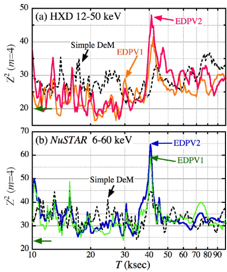
Figure 11: DeMDs ($m=4$) derived under three different conditions, from the 12–50 keV HXD data (panel a) and the 6–60 keV NuSTAR data (panel b). The result of the simple demodulation with Equation (4) is in dashed black, that with the EDPV1 correction is in orange or light green, and the EDPV2 result is in red or blue. As $T$ is varied, $P$, $A$, and $\psi_{0}$ are allowed to vary, whereas the other EDPV$i$ ($i=1$ or 2) parameters are fixed to those in Table 2, separately for the HXD and NuSTAR.

5.3.2 The 6–60 keV NuSTAR data

We applied the same EDPV1 modeling to the 6–60 keV NuSTAR data. Figure 10 (c) depicts how the pulse significance varied with $\Delta\psi$, when $T=40.5$ ks is fixed but all the other parameters ($P$, $A$, $\psi_{0}$, $E_{1}$, and $E_{2}$) are allowed to vary. The data give a clear constraint as $\Delta\psi=162^{\circ}\pm 15^{\circ}$, where the error has been determined in the same way as before. The result also reveals a pair of subsidiary peaks which are $\pm 180^{\circ}$ off the central peak, but they are lower by $\approx 5$ in heights, so that their occurrence probability is each $\sim 1/6$ of that of the central peak. This difference can be explained in the following way: if we select $\Delta\psi$ from either side peak, the coherence in $\Psi$ between the $E\leq E_{1}$ and $E\geq E_{2}$ regions becomes the same as the case with $\Delta\psi=162^{\circ}$, but the coherence in $\Psi$ must be lost between $E_{1}$ and $E_{2}$, causing a decrease in $Z_{4}^{2}$. We hence adopt the central peak, in agreement with Fig. 10 (b) and our conclusion from the HXD data. Including this $\Delta\psi$, the EDPV1 parameters from NuSTAR are given in Table 2.

We analyzed the 6–60 NuSTAR data further employing the EDPV2 corrections, and obtained the optimum parameters as given also in Table 2. Compared with the HXD results, $\Delta\psi$ and $E_{1}$ can be regarded as the same within errors, whereas $E_{2}$ and $E_{3}$ are higher. i Unlike the HXD case, $R$ became marginally positive, and its absolute value is considerably smaller. Therefore, some of the EDPV2 parameters are considered to change with time, just as $A$ varies on time scales of months to years (Makishima et al., 2019).

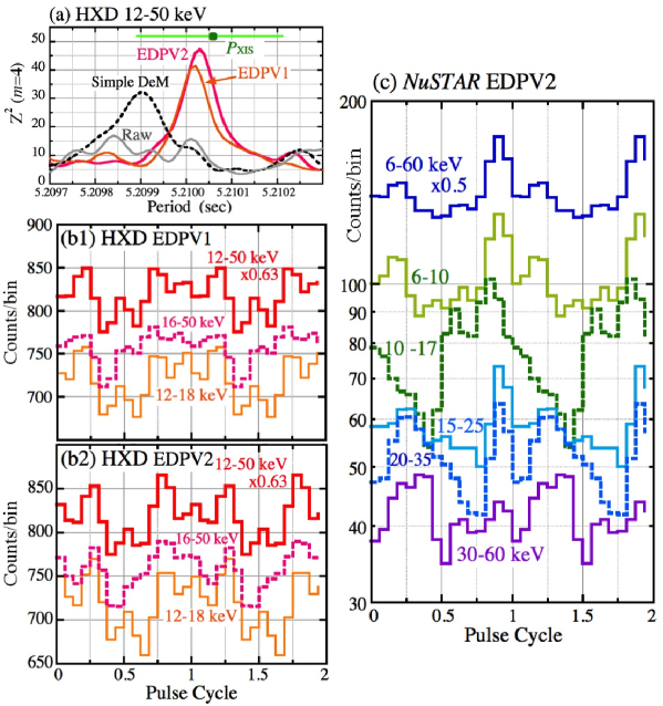
Figure 12: Results from the EDPV analysis. (a) Pulse periodograms with the 12–50 keV HXD data, computed under 4 conditions; without timing corrections (“Raw,” gray), with the simple demodulation (dashed black), the EDPV1 modeling (orange), and the EDPV2 correction (red). (b1) HXD pulse profiles with the EDPV1 scheme. (b2) Same as (b1) but with the EDPV2 correction. (c) NuSTAR pulse profiles (originally in Fig. 8) after the EDPV2 processing.

Figure 11 (b) presents the DeMDs from the 6–60 keV NuSTAR  data, calculated under the same three conditions as for the HXD data. Their basic properties are again given in Table 1. The DeMD peak has become significantly higher, from $Z_{4}^{2}=44.97$ with the simple demodulation (dashed black) to $Z_{4}^{2}=59.04$ (EDPV1; light green), and further to $Z_{4}^{2}=67.40$ (EDPV2; blue), though still smaller than that ($Z_{4}^{2}=66.51$) derived in 6–20 keV via the simple demodulation. The final value of $\psi_{0}=6^{\circ}$ agrees with $\psi=3^{\circ}$ obtained originally in 6–20 keV. In the course of these improvements, the best values of $T$, $A$, and $P$ have remained relatively unchanged. Thus, the EDPV2 modeling on the NuSTAR data has solved [N2], and at least partially [N1] as well.

So far, we used the start energy of 8 keV in the $S(E)$ formalism (equation 12), but this is somewhat arbitrarily. We hence tried changing it to 6 keV or 10 keV, to find that the case with 8 keV is slightly preferred by the NuSTAR data. (The 12–50 keV HXD data are almost insensitive.) This justifies our use of 8 keV as the start energy, both for Suzaku and NuSTAR.

5.3.3 Pulse profiles

Figure 12 (b1) shows the folded pulse profiles from the HXD data, processed through the EDPV1 scheme. Compared to the results with the simple demodulation in Fig. 7 (b2), the 16–50 keV pulse amplitude became smaller for some reasons, but the profiles became less energy dependent. They exhibit a relatively symmetric pair of horn-like peaks at $\Phi/2\pi\approx\pm 0.3$, which are similar to those found in the XIS profile in 8–12 keV (and to a lesser extent in 6–10 keV). The HXD profiles also show another pair of weaker peaks at $\Phi/2\pi\approx-0.1$ and $\approx+0.5$, and the four peaks are spaced by $\approx 1/4$ cycles. Furthermore, the 12–18 keV profile is seen to lag behind that in 16–50 keV. This “soft lag” presumably demanded the negative value of $R$. (Due to the insufficient XIS time resolution, we cannot draw any conclusion about XIS vs. HXD time lags.)

Figure 12 (b2) shows the HXD profiles corrected for the EDPV2 effect, using the parameters in Table 2 which dictate that the HXD pulse phase is most advanced at $E=(8+E_{3})/2=25.5$ keV, by $\Delta\Phi=R\,(E_{3}-8)/4=-38^{\circ}$ ($-0.11$ pulse cycles). As a result, the profiles have become mostly free from the soft lag, and exhibit the four-peak structure more clearly than before. As an assuring fact, such a four-peak profile was observed from SGR 1900+14 during its Giant Flare in 1988 (Feroci et al., 2001), and from 4U 0142+61 when demodulated (Makishima et al., 2014). On the other hand, this raises a suspicion that we might be biased towards particular EDPV2 solutions that selectively enhance the $m=4$ power. So, in Appendix B, we repeated the analysis by changing $m$, and removed this concern.

The NuSTAR pulse profiles, originally in Fig. 8, became as in Fig. 12 (c), after processed through the EDPV2 modeling. (We skip showing the EDPV1 results, because they are rather similar.) The profiles (in particular that in 10–17 keV) still depend on the energy, but they commonly exhibit a narrow peak at $\Phi/2\pi\approx-0.1$ which are nearly in phase across the entire entire energy. On both sides of this main peak, we observe secondary peaks at a separation by 1/3 to 1/4 cycles, just like in the demodulated HXD profiles (see also Appendix B).

5.3.4 Significance of the EDPV effects

The increase in the pulse significance, from the simple demodulation to the EDPV1 modeling, is $\delta Z_{4}^{2}=8.48$ and $14.07$, with Suzaku  (12–50 keV) and NuSTAR (6–60 keV), respectively. The implied decrease in $Q$ is a factor of $2.7\times 10^{-2}$ (Suzaku) and $1.9\times 10^{-3}$ (NuSTAR). Since these values are not too small, we may not readily exclude the chance origin of these improvements, when the increase in the parameters ($\Delta\psi$, $E_{1}$, and $E_{2}$) are considered. Unlike the case of the simple demodulation, it is not easy, either, to conduct any simulation studies, using the actual or Monte-Carlo-simulated data.

In spite of these limitations, we regard the EDPV1 improvements (Suzaku and NuSTAR altogether) as real, for several reasons. First, the energy-dependent changes in $\psi$ are directly visible from the data (§ 5.1; Fig. 10). Second, the EDPV1 corrections have not only increased $Z_{4}^{2}$, but also solved (at least partially) the puzzles [S1]-[S4], [N1], and [N2]. Third, the Suzaku and NuSTAR solutions agree within errors on $\Delta\psi$ and $E_{1}$, even though they differ in $E_{2}$. Such a coincidence would not easily happen if the pulse enhancements were simply due to chance fluctuations. Finally, a very similar phenomenon has already been confirmed in 1E 1547.0$-$5408 (Paper I) at broadly similar energies, from 10 to 30 keV.

The case for the EDPV2 corrections, where we further incorporate $S(E)$, is more subtle. Probably it is not very significant for NuSTAR, because $\Delta Z_{4}^{2}=5.66$ from EDPV1 to EDPV2 is rather small, in agreement with the fact that $R=0$ is marginally excluded. Actually, the apparent soft lag seen in Fig. 8, between the 6–10 and 10–17 keV profiles, was mostly rectified (though not shown) by the EDPV1 corrections, and a minor hard lag remained, which demanded $R>0$ in EDPV2. In contrast, on the HXD data, the EDPV2 scheme (with $\Delta Z_{4}^{2}=6.41$ over the previous step) is considered more effective, because it removed the 12–18 keV versus 16–15 keV soft lag (Fig. 12) which was left over by the EDPV1 step. This agree with the positive value of $R$ in the EDPV2 solution. Moreover, the 12–50 keV profile has become sharper by the EDPV2 step.

6 DISCUSSION

6.1 Summary and evaluation of the results

We analyzed the Suzaku and NuSTAR data of SGR 1900+14, acquired in 2009 and 2016, respectively. Through the epoch-folding analysis incorporating $Z_{m}^{2}$ statistics, the source pulsation in the SXC was clearly detected, with the Suzaku XIS at $P_{\rm XIS}$ (Equation 2), and with NuSTAR at $P_{\rm NuS}$ (Equation 3). In both data sets, the SXC pulses were quite regular, without evidence for any periodic phase modulation (§ 4.4).

The HXC pulses, which were not detected via simple epoch-folding analysis either with the Suzaku HXD or NuSTAR (§ 3.3; Fig. 3 b; Fig. 4 c), have been detected significantly by both these instruments through the demodulation correction (§ 4.2; Fig. 5; Fig. 6). Specifically, the 6–20 keV NuSTAR data revealed a prominent $Z_{4}^{2}$ increase at $T=40.5$ ks (Equation 8) with a chance probability of $Q_{\rm NuS}=1\%$ (§ 4.2.4), and the 8–12 keV XIS data on the HXC indicated a consistent $T$ (§ 4.2.1). The DeMD with the 16–50 keV HXD data also revealed a clear peak, with $Q_{\rm HXD}=4\%$ (§ 4.2.2),

If we were allowed to regard the HXD and NuSTAR results as the same phenomenon, the overall chance probability of our finding would be

$$Q_{\rm tot}=Q_{\rm HXD}\times Q_{\rm NuS}=4\times 10^{-4}$$ (13)

which is extremely low. However, the HXD-indicated $T=43.5$ ks (Equation 6) is somewhat inconsistent with those from the XIS and NuSTAR  [S3] (Table 1). Further inconsistencies were found between the XIS and HXD [S4], within the HXD data [S1,S2], and within those of NuSTAR [N1,N2]. The energy-dependent pulse-phase shift was identified as yet another issue [SN1]. Thus, the simple energy-independent pulse demodulation was only partially successful in recovering the HXC pulses, so Equation (13) needs some reservations.

Assuming that the HXC pulses are subject to EDPV effects, we attempted further arrival-time corrections (§ 5.2), employing two functions $\psi(E)$ and $S(E)$, which describe the pulse-pattern shifts in the $\Psi$ and $\Phi$ directions, respectively. Using the 12–50 keV HXD data and the 6–60 keV NuSTAR data as fiducial energy ranges, and guided by preliminary studies (§ 5.1), we identified the EDPV1+2 parameters (separately for Suzaku and NuSTAR; Table 2) that maximize the pulse significance, and solved the puzzles [S1], [S2], [N1], and [N2]. The EDPV1+2 corrections also brought the XIS and HXD pulse periods into an agreement, identified $T=40.5$ ks as a common periodicity, and aligned up the pulse profiles from either data set throughout the energy. Thus, [S3], [S4], and [SN1] have been solved.

In the above analyses, the EDPV1+2 parameters have been determined solely to maximize $Z_{4}^{2}$ for the HXC signals in the respective fiducial energies; no attempt was made to bring $T$, the most fundamental parameter, in agreement among the different instruments. Nevertheless, the agreement on $T$ has been achieved automatically. Therefore, the two observations are considered to have witnessed the same phenomenon. Then, we are allowed to quote Equation (13) in its face value, and conclude that the HXC pulse-phase modulation is real, rather than due to statistical fluctuations.

These results have the following meanings, which affirmatively answer the three objectives described in § 1.

1. The presence of a significant pulse-phase modulation in the HXC, and its absent in the SXC, agree with the behavior of 4U 0142+61 and 1E 1547.0$-$5408. Thus, SGR 1900+14 provides a third example to show this behavior. Our conjecture, that the phenomenon should be detected from nearly all magnetars, was reinforced.

2. The pulse-phase modulation of the HXC exhibits significant energy dependences, i.e., the changes in $\psi$ by $\Delta\psi\sim 180^{\circ}$ across an energy interval from $\approx 13.5$ keV to 15.8-21.0 keV. These effects, first seen in 1E 1547.0$-$5408 (Paper I), are hence suggested to be not rare among magnetars.

3. The Suzaku and NuSTAR  results agree on essential features of the phenomenon, including its energy dependence. This mitigates the risk of instrument-specific artifacts. They however differ in some details (e.g., on $E_{2}$ and $R$); the phenomenon is hence considered time variable to some degree.

6.2 Interpretations of the Results

6.2.1 Dynamics of an axially-symmetric rigid body

As developed through a series of our studies, the phase modulation of the HXC pulses, which is now confirmed in SGR 1900+14, can be described using the basic dynamics of an axisymmetric rigid body. Namely, we identify $T=40.5$ ks with the slip period of the NS in SGR 1900+14, which is axially elongated by $\epsilon\approx P/T=1.3\times 10^{-4}$ and performs free precession. The deformation can be ascribed to the stress by extreme $B_{\rm t}$ which reaches $\sim 10^{16}$ G.

To be more concrete, consider two Cartesian frames with a common origin (Fig.18 of Makisima et al. 2021); an inertial frame $\Sigma=(\hat{X},\hat{Y},\hat{Z})$ with the unit vector $\hat{Z}$ parallel to ${\bf L}$, and $\Sigma^{*}=(\hat{x}_{1},\hat{x}_{2},\hat{x}_{3})$ fixed to the NS. As before, $\hat{x}_{3}$ is identified with the NS’s symmetry axis. The triplet $(\Phi,\alpha,\Psi)$ provides the three Euler angles, which specify the instantaneous attitude of $\Sigma^{*}$ relative to $\Sigma$. While $\alpha$ is constant, $\Phi$ and $\Psi$ both vary. Every time $\Phi$ completes its one cycle (in the period $P_{\rm pr}$, or one pulse), $\Psi$ advances by $2\pi\epsilon\cos\alpha=2\pi(P_{\rm pr}/T)$ (§ 1). Assuming $\cos\alpha\approx 1$, $\Psi$ returns to its initial value in the slip (or beat) period $T$, which comprises $T/P_{\rm pr}$ precession cycles and $(T/P_{\rm pr})+1$ rotations around $\hat{x}_{3}$.

We further assume that the X-ray emission pattern at each energy is constant when described in the $\Sigma^{*}$ coordinates, and the changes of $\Sigma^{*}$ relative to $\Sigma$ are responsible for all observed variability, including the pulsation and its phase modulation. When the emission pattern is symmetric around $\hat{x}_{3}$, and hence independent of $\Psi$, the pulsation will be strictly periodic, like what we observe for the SXC. If instead the emission breaks symmetry around $\hat{x}_{3}$ (and hence in $\Psi$), the pulse-peak phase becomes dependent on $\Psi$, as modeled by Equation (4) in the simplest case, and actually exhibited by the HXC from SGR 1900+14.

In short, the pulses from a rotating NS become phase-modulated when the following three symmetry breakings all take place; (i) $\alpha\neq 0$, (ii) $\epsilon\neq 0$, and (iii) an asymmetric emission pattern around $\hat{x}_{3}$. The HXC of the relevant magnetars is thought to satisfy all these conditions, whereas the SXC only (i) and (ii). These clear distinctions between the SXC and HXC, in their timing behavior and their spectral shapes, suggest a fundamental difference in their origins.

6.2.2 A possible geometry

The above general conditions can be satisfied by a specific geometry given in Paper I, which also affords an explanation of the EDPV effects. Suppose that the SXC is emitted by a region symmetric around $\hat{x}_{z}$, whereas the HXC, arising via, e.g., the two-photon process, has a conical beam pattern around $\hat{x}_{z}$. The cone brightness is assumed to vary with $\Psi$ (the cone azimuth) due, e.g., to the presence of local multipoles which break the symmetry around $\hat{x}_{z}$. Then, the pulse-phase modulation up to $A\sim P/4$ can be explained in a semi-quatitative way (Paper I). Furthermore, let the directional vector $\hat{\xi}$ represent the generatrix along which the HXC is brightest. If $\hat{\xi}$ moves in $\Psi$ with energy, due to some strong-field physics such as proton cyclotron resonances (Paper I), the EDPV1 effects can be explained.

As mentioned in Paper I, the EDPV2 effect represented by $S(E)$ is more difficult to interpret. To see this, let $\Pi_{3}$ be the plane defined by $\hat{Z}\|{\bf L}$ and $\hat{x}_{3}$, which rotates around $\hat{Z}$ with a period $P_{\rm pr}$. Then, $\hat{\xi}$ as defined above, rotates relative to $\Pi_{3}$ with a period $T$, in which it crosses $\Pi_{3}$ twice. At every crossing, the pulse arrival-time delay $\delta t$ will change its sign. When averaged over a cycle, we expect $\langle\delta t\rangle\approx 0$, or $S(E)\approx 0$, as long as Equation (4) provides a good approximation. However, if the time profile of $\delta t$ is much deviated from a sinusoid, and asymmetric between $\delta t>0$ and $\delta t<0$, we may expect $S(E)\neq 0$. Thus, we tentatively regard $S(E)$ as a modeling artifact, which would vanish when we improve Equation (4). Such attempts were already made in Paper I, but only very preliminarily.

6.2.3 Implications for the nature of magnetars

So far, we have adopted the interpretation of mangetars as isolated NS powered by magnetic energies (Mereghetti, 2008). Some alternative models however describe them as NSs with ordinary dipole magnetic fields as $B_{\rm d}\sim 10^{12}$ G, powered by mass accretion from fossil or fallback disks around them (e.g. Benli and Ertan, 2016). In fact, infrared observations provided evidence for such disks around some magnetars, including 4U 0142+61 in particular (e.g. Wang et al., 2006).

Based on the disk-accretion scenario, Grimani (2021) argued that the 55 ks modulation in 4U 0142+61 can be explained when the source is hidden periodically by the disk if it is in a Keplerian rotation and is free-precessing. However, the disk is so distant (Appendix C) that the emission region would look point-like, and the disk is not highly ionized. Then, the modulation must get stronger towards lower energies because of the increasing photo-absorption, contradicting to the general absence of phase modulation in the SXC pulses. Therefore, this scenario would work for neither 4U 0142+61, nor SGR 1900+14 which is in a similar condition. Some other mechanisms must be sought for if the observed phenomenon it to be explained by the disk-accretion scenario.

Regardless of details of the phase-shift production, the EDPV effects in the two objects must be explained. Taking SGR 1900+14 for example, the 12 keV pulses at a particular phase in $\Psi$ need to arrive by $\sim 1$ s earlier than expected, whereas the 20 keV pulses later by a similar amount (Fig. 10). Such a sharp energy dependence is incompatible with the broadband nature of X-rays from accretion columns, wherein the $\sim 12$ keV and $\sim 20$ keV photons must behave in positively correlated ways. In contrast, our scenario based on the strong-field physics (§ 6.2.2) can explain the essential timing properties of SGR 1900+14 including its EDPV behavior. Therefore, the X-rays produced via accretion, if any, should contribute little to the overall X-ray emission.

We also examined how a circum-stellar disk affects the NS dynamics by forced precession. This may take place through two channels; one is via the accretion torque, wherein the NS can be spherical but needs to be accreting. The other is via direct gravity; the NS needs to be deformed, but the accretion is not required. As given in Appendix C, the former mechanism predicts a long period of forced precession as $\sim 2\times 10^{3}$ yr, whereas the latter is even longer by many orders of magnitude. Thus, the rigid-body dynamics of these magnetars are not affected by the disks around them.

Although we have argued against the accretion scenario, we do not mean that NSs with $B_{\rm d}\gtrsim 10^{14}$ G cannot become accreting sources, or cannot reside in binaries. In fact, the binary X-ray pulsar X-Persei, accreting from the companion’s stellar winds, has been found to have $B_{\rm d}\sim 1\times 10^{14}$ G (Yatabe et al., 2018). As another interesting case, the gamma-ray binary LS 5039 is likely to harbor a non-accreting magnetar, whose magnetic energy is released via interactions with the primary’s stellar winds to drive the remarkable non-thermal activity (Yoneda et al., 2020, 2021). Yet another example is so-called Central Compact Objects (CCOs), rather inactive NSs found at the center of some supernova remnants (e.g. Esposito et al., 2019). They are thought to have weak $B_{\rm d}$ but intense $B_{\rm t}$, and the latter sustains their activity. Thus, a fair fraction of NSs may be born as magnetars in a broad sense (Nakano et al., 2015), and reside in various environments. As suggested by the present study, some, if not all, of them might have $B_{\rm t}\sim 10^{16}$ G. It would hence be an interesting future work to classify magnetized NSson the $(B_{\rm d},B_{\rm t})$ plane.

6.3 4U 1626$-$67 as a counter example

The confirmed phase-modulation period $T$ is rather similar among the three objects; 55 ks in 4U 0142+61, 36 ks in 1E 1547.0$-$5408, and 40.5 ks in SGR 1900+14. Then, a concern arises; could this effect be some instrumental or observational artifacts in hard X-rays, and emerge virtually in all X-ray pulsars? As a candidate counter example, we studied the ultra-compact binary pulsar 4U 1626$-$67, because its pulse period, 7.68 s, is similar to those of magnetars, and its orbital Doppler effect is very small as $<13$ lt-ms (Levine et al., 1988).

On 2006 March 9 through 11 (ObsID 40015010), 4U 1626$-$67 was observed with Suzaku for an elapsed time of 239 ks. The data were already analyzed by Iwakiri et al. (2012), who detected the pulsation at $P=7.67795(9)$ s. We processed these HXD data in the same way as for SGR 1900+14, including the barycentric correction, and applied the demodulation analysis to the 12–34 keV and 34–40 keV events. The former energy range enables us to utilize the highest data statistics, whereas the latter to emulate the pulse significance actually observed from SGR 1900+14.

The DeMDs from 4U 1626$-$67 are shown in Fig. 13. In panel (a) for 12–34 keV, $Z_{4}^{2}$ takes extremely large values with the mean of $\langle Z_{4}^{2}\rangle=14,827$, reflecting high signal statistics. Nevertheless, the DeMD does not show outstanding peaks, and varies only by $\pm 1.80$ (1$\sigma$) which is smaller than the Poissonian prediction (§ 4.4). Moreover, the modulation amplitude is tightly constrained as $A\lesssim 0.04$ s ($\lesssim 0.5\%$ of $P$) throughout.

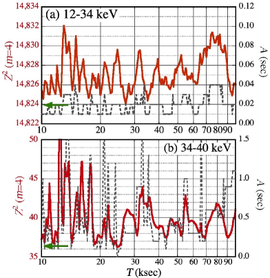
Figure 13: DeMDs ($m=4$) from the Suzaku HXD data of 4U 1626$-$67, in the (a) 12–34 keV and (b) 34–40 keV intervals. The plot style is the same as for Fig. 5.

Similarly, the 34–40 keV DeMD in Fig. 13 (b) has a 1$\sigma$ variation by $\pm 2.66$, without significant peaks except in 12–18 ks where multiples of the Suzaku’s orbital period appear. Here, $A$ takes much larger values than in panel (a), for the following reason (Makishima et al., 2016). In general, increasing $A$ has two opposite effects; to degrade the underlying pulse coherence, and to increase the number of different combinations of the Poisson fluctuations. When the pulsation has high significance, the former effect dominates to favor small values of $A$, whereas the opposite occurs when the underlying pulsation has low statistics.

The two DeMDs in Fig. 13 can thus be interpreted both as a sum of a regular pulsation and Poissonian fluctuations, with no evidence for intrinsic pulse-phase modulation over the 10–100 ks interval. This conclusion remains unaffected even if using various different energy intervals, or extending the search range of $T$ up to $\sim 500$ ks (beyond which the data are no longer constraining). Therefore, 4U 1626$-$67 provides a good counter example to our concern, and suggests that the pulse-phase modulation is an effect specific to the HXC of magnetars, rather than some observational artifacts.

In terms of the rigid-body dynamics, the negative result on 4U 1626$-$67 can be explained by logically inverting the three symmetry-breaking conditions described in § 6.2.1, and restoring the individual symmetry. That is, the phase modulation will vanishes if (i^′) $\alpha\approx 0$ (aligned rotators), or (ii^′) $\epsilon\approx 0$ (spherical symmetry), or (iii^′) $\vec{\xi}\|\hat{x}_{3}$. Among the three options, (i^′) is ruled out because the source is pulsing. Next, consider (ii^′). Since 4U 1626$-$67 has $B_{\rm d}\approx 3\times 10^{12}$ G (Iwakiri et al., 2012), it would be very likely to have $B_{\rm t}\ll 10^{16}$ G. Then, the NS should be nearly spherical with $\epsilon\ll 10^{-4}$, satisfying (ii^′). In this case, Equation (1) indicates $T\gg 10^{4}P_{\rm pr}$. Then, during a typical observation, $\vec{\xi}$ is phase-locked to the $\Pi_{3}$ plane, and the pulses will keep a constant phase. Finally, let us consider (iii^′). The X-rays from accreting pulsars are produced in their accretion columns mainly via thermal Compntonization, modified by electron cyclotron resonances. So the emission would be azimuthally isotropic, even though otherwise in the polar direction. Therefore, (iii^′) is also likely to hold.

To summarize, the emission from accreting pulsars, including 4U 1626$-$67, is in a condition (i)$\land$(ii^′)$\land$(iii^′), where $\land$ means logical and. In contrast, the SXC and HXC of magnetars are expressed by (i)$\land$(ii)$\land$(iii^′) and (i)$\land$(ii)$\land$(iii), respectively. As a result, the pulse-phase modulation is observed only from the HXC of magnetars. These characterizations highlight the intrinsic difference between the magnetically-powered and accretion-powered NSs.

7 CONCLUSION

1. In hard X-rays, the 5.2-s pulsation of SGR 1900+14 was not detected at first, with either Suzaku or NuSTAR. However, the pulses became detectable by correcting the photon arrival times for the phase-modulation effects, assuming a period of $T=40.5\pm 0.8$ ks as consistently indicated by the Suzaku XIS, Suzaku HXD, and NuSTAR. Thus, SGR 1900+14 becomes a third example that shows this behavior, after 4U 0142+61 and 1E 1547.0$-$5408.

2. We identify $T$ with the slip period associated with free precession of the NS, which is axially deformed to $\epsilon\approx P/T=1.3\times 10^{-4}$, presumably by the stress of $B_{\rm t}\sim 10^{16}$ G. The observed value of $A\approx 1.0$ s is consistent with this picture.

3. A series of problems, left by the simple demodulation, were mostly solved by considering the EDPV effects, like in the NuSTAR data of 1E 1547.0$-$5408. The derived EDPV parameters partially agree between Suzaku and NuSTAR.

4. The pulse-phase modulation is not likely to be an observational artifact, because it was absent in the Suzaku data of a counter example, 4U 1626$-$67.

5. This phenomenon is possibly ubiquitous among magnetars, and will provide valuable clues to their $B_{\rm t}$, as well as to their HXC emission mechanism which must be distinct from that of the SXC.

6. The present results favor the interpretation of magnetars as magnetically powered NSs, rather than as those accreting from circumstellar disks.

7. Intense toroidal agnetic fields, up to $B_{\rm t}\sim 10^{16}$ G, could be rather common among magnetars and similar NSs.

Appendix A: Statistical significance of the phase modulation

By the simple energy-independent demodulation analysis in § 4.2, we obtained $Z_{4}^{2}=40.64$ and $Z_{4}^{2}=66.51$, from the 16–50 keV HXD data and the 6–20 keV NuSTAR  data, respectively (Table 1). Referring to the chi-square distribution with $2m=8$ degrees of freedom, the chance occurrence probability becomes $Q_{\rm HXD}^{0}=2.4\times 10^{-6}$ (HXD) and $Q_{\rm NuS}^{0}=2.4\times 10^{-11}$ (HXD). Although the significance appears to differ by many orders of magnitude between the two results, the difference is in reality not so large, because in terms of the increment, the NuSTAR peak has $\delta Z_{4}^{2}=29.35$ whereas that of the HXD is $\delta Z_{4}^{2}24.07$, with a difference of only 5.28.

To evaluate the true statistical significance of the detected effect, we must consider two additional factors (Makishima et al., 2016). One is that these values must be multiplied by the total number of independent trials (difficult to estimate) involved in the DeMDs in Fig. 5. The other is that the above estimates of $Q$ are valid only when the signal is purely Poissonian, and needs revisions when the signal is already pulsing before the demodulation. Hence, we developed several methods to estimate the true significance (Makishima et al. (2014, 2016), Paper I), mainly using the actual data but partially incorporating Monte-Carlo technique.

Adopting the method in Paper I, we repeated the same demodulation analysis over an interval of $T=0.05-3.0$ ks, which is shorter than the orbital period of Suzaku but still longer than the pulse period. We varied the scan steps in $T$ as $\Delta T=T^{2}/T_{\rm tot}$, where $T_{\rm tot}=114$ ks is the total observation time lapse. This $\Delta T$ is the smallest step that ensures the independence between adjacent sampling points in terms of Fourier wave numbers. We have thus obtained $2242$ ($=114/0.05-114/3.0)$ steps in $T$, which is 219 times larger than that in the actual DeMD calculation over the $T=10.0-100$ ks interval, namely, $114/10.0-114/100=10.26$. We scanned $P$, $A$, and $\psi$ over the same ranges and same steps as in deriving Fig. 5 (a2), so that the trial numbers in these quantities are the same. Through this control study, $Z_{4}^{2}$ exceeded the target value $Z_{4}^{2}=40.64$ at 8 values of $T$. Therefore, the probability for the 43.5 ks peak in the 16–50 keV DeMD to appear by chance finally becomes $Q_{\rm HXD}=8/219\approx 4\%~{}.$

We conducted the control study using the 6–20 keV NuSTAR  data as well, exactly in the same manner as for the HXD data, but with $\Delta T$ halved because of the twice longer $t_{\rm tot}$. The ratio of 219, between the control study and the DeMD in Fig. 5 (b1), remains the same. (In calculating the latter, $T$ is over-sampled.) As a result, the control study yielded two ponts in $T$ where $Z_{4}^{2}$ exceeds the target value of 66.51. Therefore, the chance probability for the 40.5 ks peak in the 6–20 keV NuSTAR DeMD is estimated as $Q_{\rm NuS}=2/219\approx 1\%~{}$ which is lower, as expected, than $Q_{\rm HXD}$.

Appendix B: Effects of the Fourier harmonic number

To examine whether our results are biased by our choice of $m=4$, we repeated the EDPV2 analysis on the 12–50 keV HXD data, by changing $m$ from 1 to 8, and re-optimizing the EDPV2 parameters at each $m$. The obtained values of $Z_{m}^{2}$ are given Table 3, together with the difference $\Theta_{m}\equiv Z_{m}^{2}-Z_{m-1}^{2}$ which represents the $m$-th Fourier power of the pulse profile. For a purely Poissonian signal, we expect $\Theta_{m}\approx 2$ regardless of $m$. Thus, the highest power is in $m=4$, and then in $m=8$, both in agreement with the pulse profiles in Fig. 12.

As for the 6–60 keV NuSTAR data, the same scan in $m$ gave $\Theta_{m}=28.3,4.6,18.5$, and 12.4, for $m=1,2,3$, and 4, respectively. Thus, the 4th harmonic is somewhat weaker than the 3rd. Nevertheless, our choice of $m=4$ for the NuSTAR data is considered appropriate, because we found $\Theta_{m}\lesssim 3$ for $m\geq 5$.

Table 3: Maximum values of $Z_{m}^{2}$ from EDPV2 analysis of the 12–50 keV HXD data, as a function of $m$ (see text).

$m$	1	2	3	4	5	6	7	8
$Z_{m}^{2}$	14.2	25.5	31.6	48.0	49.6	50.9	54.9	63.1
$\Theta_{m}$	14.2	11.3	6.1	16.4	1.6	1.3	4.0	8.2

Appendix C: Forced precession induced by a circum-stellar disk

Of the two modes of forced precession induced by a circum-stellar disk (§ 6.2.3), the accretion-induced effect will take place on a time scale which is comparable to the spin-up time scale of the NS, $\tau_{\rm su}$. According to Ghosh and Lamb (1979), it is estimated as

$$\tau_{\rm su}\sim 3\times 10^{4}P({\rm sec})^{-1}\mu_{30}^{-2/7}\,L_{36}^{-6/7}~{}{\rm yr}$$

where $\mu_{30}$ is the magnetic moment of the NS in $10^{30}$ cgs units, and $L_{36}$ is the accretion luminosity in units of $10^{36}$ erg s^-1. Then, even if assuming the most favorable conditions that $L_{36}\sim 0.55$ of SGR 1900+14 is totally due to accretion, and yet the NS has $B_{\rm d}\sim 10^{14}$ G implying $\mu_{30}\sim 100$, a rather long time scale as $\tau\sim 2\times 10^{3}$ yr is indicated.

The other mode, namely, the direct gravitational perturbation on an axially deformed NS, was studied by Tong et al. (2020). In this case, the period of forced precession of the NS is given as

$$P_{\rm forced}=(16\pi^{2}R^{3})/(9GM_{\rm d}\epsilon P)$$

(adapted from Equation 2 of Tong et al. (2020)) where $G$ is the gravitational constant, $M_{\rm d}$ is the total disk mass, and $R$ is a representative disk radius. For simplicity, we assumed that the disk normal is parallel to $\bf{L}$. If considering the disk around 4U 0142+61, Wang et al. (2006) give $M_{\rm d}\sim 6\times 10^{28}$ g and $R\sim 4\times 10^{11}$ cm. These, together with $\epsilon\sim 10^{-4}$ from our measurements and $P=8.96$ s, yield $P_{\rm forced}\sim 10^{9}$ yr. Therefore, the effect is totally negligible. Although the estimate may change to some extent when considering the disk wobbling, the conclusion would remain unaffected.

References

- Benli and Ertan (2016) Benli, O., Ertan, Ü. 2016, MNRAS, 457, 4114
- Brazier (1994) Brazier K. T. 1994, MNRAS, 268, 709
- Davies et al. (2009) Davies, B., Figer, D. F., Kudritzki, R., Trombley, C., Kouveliotou, C, Wachter, S. 2009, ApJ, 707, 844
- Enoto et al. (2017) Enoto T. et al. 2017, ApJS, 231, 8
- Enoto et al. (2010) Enoto T., Nakazawa K., Makishima K., Rea N., Hurley K., Shibata S. 2010, ApJ, 722, L162
- Esposito et al. (2019) Esposito, P., et al. 2019, A&A, 326, id.A19
- Feroci et al. (2001) Feroci M., Hurley K., Duncan R. C., Thompson C. 2001, ApJ, 549, 1021
- Ghosh and Lamb (1979) Ghosh, P., Lamb, F. K. 1979, ApJ, 234, 296
- Grimani (2021) Grimani, C. 2021, MNRAS, 507, 261
- Iwakiri et al. (2012) Iwakiri, B. E. et al. 2012, ApJ, 751, 5
- Kokubun et al. (2007) Kokubun M. et al. 2007, PASJ, 59, S53
- Koyama et al. (2007) Koyama, K. et al. 2007, PASJ, 59, S23
- Kuiper et al. (2006) Kuiper L., Hermsen W., den Hartog P., Collmar W. 2006, ApJ, 645, 556
- Levine et al. (1988) Levine, A. Ma, C. P., McClintock, J., Rappaport, S., van der Klis, M, Verbunt, F. 1988, ApJ, 327, 732
- Makishima (2016) Makishima K. 2016, Proc. Japan Academy, Ser. B, 92, 135
- Makishima et al. (2014) Makishima K., et al. 2014, Phys. Rev. Lett., 112, 171102
- Makishima et al. (2016) Makishima K., Enoto T., Murakami H., Furuta Y., Nakano T, Sasano M., Nakazawa, K. 2016, PASJ, 68S, 12
- Makisima et al. (2021) Makishima, K., Enoto, T., Yoneda, H., Odaka, H. 2021, MNRAS, 502, 2266
- Makishima et al. (2019) Makishima K., Muakami H., Enoto T., Nakazawa K. 2019, PASJ, 71, 15 (Paper I)
- Mereghetti (2008) Mereghetti, S. 2008, A&AR, 15, 225
- Nakagawa et al. (2009) Nakagawa Y. E., Yoshida A., Yamaoka K., Shibazaki, N. 2009, PASJ, 61, 109
- Nakano et al. (2015) Nakano, T., et al. 2015, PASJ, 67, id.9
- Takahashi et al. (2007) Takahashi T., et al. 2007, PASJ, 59, S35
- Tamba et al. (2019) Tamba T., Bamba, A., Odaka, H,, Enoto, T. 2019, PASJ, 71, id.90
- Tong et al. (2020) Tong, H., Wang, W., Wang, H.-G, 2020, Res. Astr. Ap., 20, 142
- Wang et al. (2006) Wang, Z., Chakrabarty, D., Kaplan, D. L. 2006, Nature, 440, 772
- Yatabe et al. (2018) Yatabe, F., et al. . 2018, PASJ, 70, id.89
- Yoneda et al. (2020) Yoneda, H., et al. 2021, ApJ, 917, id.90
- Yoneda et al. (2021) Yoneda, H., Makishima, K., Enoto, T., Khangulyan, D., Matsumoto, T., Takahashi, T. 2020, Phys. Rev. Lett., 125, id.111103