Conditional Poisson Stochastic Beam Search

Abstract

Beam search is the default decoding strategy for many sequence generation tasks in NLP. The set of approximate $K$-best items returned by the algorithm is a useful summary of the distribution for many applications; however, the candidates typically exhibit high overlap and may give a highly biased estimate for expectations under our model. These problems can be addressed by instead using stochastic decoding strategies. In this work, we propose a new method for turning beam search into a stochastic process: Conditional Poisson stochastic beam search. Rather than taking the maximizing set at each iteration, we sample $K$ candidates without replacement according to the conditional Poisson sampling design. We view this as a more natural alternative to Kool et al. (2019)’s stochastic beam search (SBS). Furthermore, we show how samples generated under the CPSBS design can be used to build consistent estimators and sample diverse sets from sequence models. In our experiments, we observe CPSBS produces lower variance and more efficient estimators than SBS, even showing improvements in high entropy settings.

1 Introduction

Many NLP tasks require the prediction of structured outputs, such as sentences or parse trees, either during decoding or as part of a training algorithm. For today’s neural architectures, beam search Reddy (1977) has become the decoding algorithm of choice due to its efficiency and empirical performance Serban et al. (2017); Edunov et al. (2018); Yang et al. (2019); Meister et al. (2020b). Beam search is a deterministic method, which invites a natural question: What is the proper stochastic generalization of beam search? Several recent papers have investigated this question Kool et al. (2019, 2020); Shi et al. (2020). Here we build on this line of work and introduce an alternative stochastic beam search that the authors contend is a more faithful stochasticization of the original algorithm in that it recovers standard beam search as a special case. We name our algorithm conditional Poisson stochastic beam search (CPSBS) as we draw on the conditional Poisson sampling scheme Hájek (1964) in its construction. The relationship between CPSBS and other common decoding strategies is displayed visually in Table 1.

At every iteration, CPSBS replaces the top-$K$ operator in the beam search algorithm with conditional Poisson sampling, resulting in a decoding strategy that generates samples-without-replacement. Importantly, annealing our sampling distribution at each time step turns local sampling into a local top-$K$ computation and thereby recovers beam search. We subsequently show that these samples can be used to construct a statistically consistent estimator for the expected value of an arbitrary function of the output.

3  $K=1$ $K>1$   $\mathrm{argmax}$ Greedy Search Beam Search   Ancestral Conditional $\mathrm{sample}$ Sampling Poisson Beams  

Table 1: A comparison of beam-based decoding algorithms for sequence models, by solution set size and objective. The $\operatorname*{argmax}$ and sample variants are related through annealing: As the annealing parameter of the distribution $\tau\!\rightarrow\!0$, sampling turns into computing an $\operatorname*{argmax}$ (see § 3).

In our experiments with neural machine translation models, we observe that CPSBS leads to better estimates of expected bleu and conditional model entropy than SBS and the sum-and-sample estimator Kool et al. (2020), distinctly outperforming Monte Carlo sampling for both small sample sizes and low temperatures. Furthermore, we find that CPSBS can be used as a diverse sampling strategy. We take these results as confirmation that CPSBS is a useful tool in the newfound arsenal of sampling strategies for neural sequence models.

2 Beam Search

In this section, we overview the necessary background on neural sequence models and beam search in order to motivate our algorithm in § 3.

Neural Sequence Models.

We consider locally normalized probabilistic models over sequences $\mathbf{y}$:

$$p(\mathbf{y})=\prod_{t=1}^{|\mathbf{y}|}p(y_{t}\mid\mathbf{y}_{<t})$$ (1)

where $\mathbf{y}$ is a member of a set of well-formed outputs $\mathcal{Y}$. In the context of language generation models, well-formed outputs are sequences of tokens $\mathbf{y}=\langle y_{1},y_{2},\dots\rangle$ from a vocabulary $V$; all $\mathbf{y}\in\mathcal{Y}$ begin and end with special tokens bos and eos, respectively. We use $\mathbf{y}_{<t}$ to represent the subsequence $\langle y_{1},\dots,y_{t-1}\rangle$. In this work, we consider the setting where the maximum sequence length is upper-bounded; we denote this upper bound $T>0$. Without loss of generality, we may condition $p$ on an input $\mathbf{x}$, as is necessary for machine translation and other conditional generation tasks.

Beam Search.

Beam search is a commonly used search heuristic for finding an approximate solution to the following optimization problem:

$$\mathbf{y}^{\star}=\operatorname*{argmax}_{\mathbf{y}\in\mathcal{Y}}\,\log p(\mathbf{y})$$ (2)

Its most straightforward interpretation is as a pruned version of breadth-first search, where the breadth of the search is narrowed to the top-$K$ candidates. However, here we will present beam search in a nonstandard lens Meister et al. (2020a, 2021) in order to emphasize the connection with our stochastic generalization in § 3. Specifically, we present the algorithm as iteratively finding the highest-scoring set under a specific set function.

Under this paradigm, the initial beam $Y_{0}$ contains only the bos token. At subsequent steps $t=1,\ldots,T$, beam search selects the $K$ highest-scoring candidates from the set $Y_{t-1}\circ V$ that we define below:

$$Y_{t-1}\circ V\mathrel{\stackrel{{\scriptstyle\textnormal{def}}}{{=}}}\{\mathbf{y}\circ y\mid\mathbf{y}\in Y_{t-1}\textbf{ and }y\in V\}$$ (3)

where $\circ$ is sequence concatenation. Those candidate sets with collectively higher probability under the model $p$ have higher score. This process continues until all $\mathbf{y}\in Y_{t}$ end in eos, or $t=T$. For notational ease, we define $B_{t}\mathrel{\stackrel{{\scriptstyle\textnormal{def}}}{{=}}}Y_{t-1}\circ V$; throughout this paper, we will assume $|B_{t}|=N$ and identify the elements of $B_{t}=\{\mathbf{y}_{\leq t}^{(1)},\ldots,\mathbf{y}_{\leq t}^{(N)}\}$ with the integers $\{1,\ldots,N\}$.

We can formulate the time-step dependent set function whose $\operatorname*{argmax}$ beam search finds as

$$Q_{t}(Y_{t}\mid Y_{t-1})\!\mathrel{\stackrel{{\scriptstyle\textnormal{def}}}{{\propto}}}\!\begin{cases}\prod_{n\in Y_{t}}w_{n}&\textbf{if }|Y_{t}|\!=\!K\\ 0&\textbf{otherwise}\end{cases}$$ (4)

where $w_{n}$ is the weight of the $n^{\text{th}}$ element of $B_{t}$. To recover beam search, we set our weights equal to probabilities under a model $p$, i.e., $w_{n}=p\!\left(\mathbf{y}_{\leq t}^{(n)}\right)$. Note that we leave the constraint that $Y\subseteq B_{t}$ implicit in Eq. 4. As should be clear from notation, this set function only assigns nonzero scores to subsets of $Y_{t-1}\circ V$ of size exactly $K$ and the assigned score is proportional to the product of the probability of the candidates under the model $p$. Putting this all together, beam search may be viewed as the following iterative process:

3 Conditional Poisson Stochastic Beams

Our paper capitalizes on a very simple observation: Rather than taking its $\operatorname*{argmax}$, we may renormalize Eq. 4 into a distribution and sample-without-replacement a size $K$ set at each iteration:

This recursion corresponds to performing conditional Poisson sampling (CPS; Hájek 1964; see App. A for overview), a common sampling-without-replacement design Tillé (2006), at every time step. Thus we term this scheme conditional Poisson stochastic beam search. CPSBS gives us a probability distribution over sets of candidates of size $K$, i.e., the final beam $Y_{T}$. We denote the CPSBS distribution $P$ and we write $Y_{T}\sim P$ to indicate that $Y_{T}$ is the stochastic beam at the end of a sampling run. We may write $P(Y_{T})$ as a marginal probability, summing over all sequences of beams that could have resulted in $Y_{T}$:

$$P(Y_{T})=\sum_{Y_{1}}\!{\cdots}\!\sum_{Y_{T-1}}\prod_{t=1}^{T}Q_{t}(Y_{t}\mid Y_{t-1})$$ (11)

Note the structural zeros of $Q_{t}$ prevent any incompatible sequence of beams. We provide a theoretical analysis of the scheme in § 4 and an empirical analysis in § 5.

Normalizing $Q_{t}(\cdot\mid Y_{t-1})$.

At each time step $t$, we compute $Q_{t}(\cdot\mid Y_{t-1})$—a distribution over subsets of size $K$ of a base set $B_{t}$—using the CPS design. The normalizing constant for this distribution is defined as

$$\mathrm{Z}_{t}\mathrel{\stackrel{{\scriptstyle\textnormal{def}}}{{=}}}\sum_{\begin{subarray}{c}Y_{t}\subseteq B_{t},\\ |Y_{t}|=K\end{subarray}}\prod_{n\in Y_{t}}w_{n}\,$$ (12)

Despite there being exponentially many summands, we can sum over all ${N\choose K}$ subsets in $\mathcal{O}\!\left(NK\right)$ time via the following recurrence relation:

$$\mathrm{W}{n\choose k}=\begin{cases}1&\!\!\!\!\textbf{if }k=0\\ \mathrm{W}{n-1\choose k}+w_{n}\mathrm{W}{n-1\choose k-1}&\!\!\!\!\textbf{if }k\in(0,n)\\ 0&\!\!\!\!\textbf{otherwise }\end{cases}$$

We give complete pseudocode in App. C. Correctness of this algorithm is shown in Kulesza and Taskar (2012). The normalizing constant can then be efficiently computed as

$$\mathrm{Z}_{t}=\mathrm{W}{N\choose K}$$ (13)

Sampling from $Q_{t}(\cdot\mid Y_{t-1})$.

We can efficiently sample sets from $Q_{t}(\cdot\mid Y_{t-1})$ using the algorithm below:

1:$Y_{t}\leftarrow\emptyset$ $\triangleright$ Initialization

2:for $n=N\ldots 1$ :

3:   $k\leftarrow K-|Y_{t}|$ $\triangleright$ Number of remaining elements

4:   Add the $n^{\text{th}}$ element of $B_{t}$ to $Y_{t}$ with prob.

$$\frac{w_{n}\,\mathrm{W}{n-1\choose k-1}}{\mathrm{W}{n\choose k}}$$

5:return $Y_{t}$ $\triangleright$ Guaranteed to have size $K$

In words, the algorithm considers adding each element one at a time until $K$ elements have been sampled. Notice that line 4 adjusts the probability of sampling item $n$ given that $|Y_{t}|$ items have already been sampled, which ensures that exactly $K$ elements are sampled at termination.

Setting $w_{n}$.

The weight assigned to the $n^{\text{th}}$ item of $B_{t}$ directly affects its probability of being included in the sampled set, i.e., $\mathrm{Pr}\left(\mathbf{y}_{\leq t}^{(n)}\in Y_{t}\right)$, also termed an item’s inclusion probability. In this paper, we write $\pi_{\scaleto{Q_{t}}{5pt}}\Big{(}\mathbf{y}_{\leq t}^{(n)}\!\mid\!Y_{t-1}\Big{)}$ to denote the inclusion probability under the distribution $Q_{t}(\cdot\mid Y_{t-1})$, defined as:

$$\pi_{\scaleto{Q_{t}}{5pt}}\Big{(}\mathbf{y}_{\leq t}^{(n)} \mid Y_{t-1}\Big{)}$$ (14)

$$\mathrel{\stackrel{{\scriptstyle\textnormal{def}}}{{=}}}\sum_{Y_{t}}Q_{t}(Y_{t}\mid Y_{t-1})\mathbbm{1}\{\mathbf{y}_{\leq t}^{(n)}\in Y_{t}\}$$

One strategy is to choose $w_{n}$ at time step $t$ such that $\pi_{\scaleto{Q_{t}}{5pt}}\Big{(}\mathbf{y}_{\leq t}^{(n)}\mid Y_{t-1}\Big{)}\approx p(\mathbf{y}_{\leq t}^{(n)})$. This choice recovers beam search when we anneal our chosen weights $w_{n}\mapsto w_{n}^{1/\tau}$: as the temperature parameter $\tau\to 0$, the CP distribution will assign probability 1 to the set containing the top-$K$ elements.

Finding $w_{n}$’s that result in pre-specified inclusion probabilities is possible, but it requires solving a numerical optimization problem Aires (1999); Grafström (2009). Further, in CPSBS, we will be sampling from a different distribution at each time step and it would be quite slow to solve the numerical optimization problem each iteration. Luckily, the choice of $w_{n}=p(\mathbf{y}_{\leq t}^{(n)})/(1-p(\mathbf{y}_{\leq t}^{(n)}))$ yields a good approximation to the target inclusion probabilities in both theory and practice Hájek (1981); Bondesson et al. (2006); Aires (1999).

4 Statistical Estimation with Conditional Poisson Stochastic Beam Search

In this section, we discuss statistical estimation with CPSBS samples. To that end, we construct two estimators with different properties. However, only the second estimator provides good performance in practice, which is discussed later in § 5.

4.1 The Horvitz–Thompson Estimator

We build upon the Horvitz–Thompson (HT) estimator Horvitz and Thompson (1952), which is a common technique for estimation from sampling-without-replacement (SWOR) schemes.

Let ${f}:\mathcal{Y}\rightarrow\mathbb{R}^{d}$ be a function whose expected value under $p$ we seek to approximate:

$$\mathbb{E}_{\mathbf{y}\sim p}\left[{f}(\mathbf{y})\right]=\sum_{\mathbf{y}\in\mathcal{Y}}p(\mathbf{y}){f}(\mathbf{y})$$ (15)

The Monte Carlo estimator of the above quantity is

$$G_{\mathrm{MC}}\mathrel{\stackrel{{\scriptstyle\textnormal{def}}}{{=}}}\frac{1}{M}\sum_{m=1}^{M}f(\mathbf{y}^{(m)})$$ (16)

where $\mathbf{y}^{(m)}\overset{\mathrm{i.i.d.}}{\sim}p$. However, in the special case of sampling from a finite population—which is extremely common in NLP—it can be very wasteful. For example, if a distribution is very peaked, it will sample the same item repeatedly; this could lead to inaccurate approximations for some $f$. As a consequence, the mean square error (MSE) of the estimator with respect to $\mathbb{E}_{\mathbf{y}\sim p}\left[{f}(\mathbf{y})\right]$ can be quite high for small $M$. Indeed, we see this empirically in Fig. 2(b).

Taking samples without replacement allows us to cover more of the support of $p$ in our estimate of $\mathbb{E}_{\mathbf{y}\sim p}\left[{f}(\mathbf{y})\right]$. However, we must take into account that our samples are no longer independent, i.e., $\mathbf{y}^{(m)}\overset{\mathrm{i.i.d.}}{\not\sim}p$. We now define the HT estimator, using notation specifically for the case of CPSBS:

$$G_{\mathrm{HT}}\mathrel{\stackrel{{\scriptstyle\textnormal{def}}}{{=}}}\sum_{\mathbf{y}\in Y_{T}}\frac{p(\mathbf{y})}{\pi_{\scaleto{P}{4pt}}(\mathbf{y})}{f}(\mathbf{y})$$ (17)

As should be clear from notation, we assume $Y_{T}\sim P$; further, we use $\pi_{\scaleto{P}{4pt}}(\mathbf{y})$ to denote the inclusion probability of $\mathbf{y}$ under CPSBS, i.e., the probability of sampling a set $Y_{T}\sim P$ that contains the element $\mathbf{y}$:

$$\pi_{\scaleto{P}{4pt}}(\mathbf{y})=\sum_{Y_{T}}\!P(Y_{T})\mathbbm{1}\{\mathbf{y}\in Y_{T}\}$$ (18)

$$=\sum_{Y_{1}}\!{\cdots}\!\sum_{Y_{T}}\prod_{t=1}^{T}Q_{t}(Y_{t}\mid Y_{t-1})\mathbbm{1}\left\{\mathbf{y}_{\leq t}\in Y_{t}\right\}$$

In Eq. 17, the distribution $\pi_{\scaleto{P}{4pt}}$ may be viewed as a proposal distribution in the sense of importance sampling Owen (2013) and $1/\pi_{\scaleto{P}{4pt}}(\mathbf{y})$ as the corresponding importance weight corrections. If we can exactly compute $\pi_{\scaleto{P}{4pt}}$, then the HT estimator is unbiased (see § B.1 for proof). However, the summation in Eq. 18 is intractable so we resort to estimation.

4.2 Estimating Inclusion Probabilities

In this section, we develop statistical estimators of the inclusion probabilities under conditional Poisson stochastic beam search. Note that in order to maintain the unbiasedness of the HT estimator, we must estimate the reciprocal inclusion probabilities. However, these are not straightforward to estimate. Thus, we attempt to estimate the inclusion probabilities directly and take the reciprocal of this estimator. This strategy leads to a consistent, but biased, estimator. An important caveat: the analysis in this section only applies to the estimators of the inclusion probabilities themselves. Further analysis may be undertaken to analyze the variance of the HT estimators that make use of these estimators.

4.2.1 Naïve Monte Carlo

One obvious way to derive an inclusion probability estimator is via Monte Carlo estimation:

$$\widehat{\pi}^{\scaleto{\textsc{mc}}{3pt}}_{\scaleto{P}{4pt}}(\mathbf{y})\mathrel{\stackrel{{\scriptstyle\textnormal{def}}}{{=}}}\frac{1}{M}\sum_{m=1}^{M}\mathbbm{1}\Big{\{}\mathbf{y}\in Y_{T}^{(m)}\Big{\}}$$ (19)

where $Y^{(m)}\sim P$.

Proposition 4.1.

Eq. 19 has the following two properties:

1. $\widehat{\pi}^{\scaleto{\textsc{mc}}{3pt}}_{\scaleto{P}{4pt}}$ is an unbiased estimator of $\pi_{\scaleto{P}{4pt}}$ and

   $$\mathbb{V}\left[\widehat{\pi}^{\scaleto{\textsc{mc}}{3pt}}_{\scaleto{P}{4pt}}\right]=\frac{1}{M}\left(\pi_{\scaleto{P}{4pt}}(\mathbf{y})-\pi_{\scaleto{P}{4pt}}(\mathbf{y})^{2}\right)$$ (20)

2. ${1}/{\widehat{\pi}^{\scaleto{\textsc{mc}}{3pt}}_{\scaleto{P}{4pt}}}$ is a consistent estimator of ${1}/{\pi_{\scaleto{P}{4pt}}}$ with asymptotic variance

   $$\mathbb{V}_{\mathrm{a}}\left[\frac{1}{\widehat{\pi}^{\scaleto{\textsc{mc}}{3pt}}_{\scaleto{P}{4pt}}(\mathbf{y})}\right]\!=\!\frac{1}{M}\left(\frac{1}{\pi_{\scaleto{P}{4pt}}(\mathbf{y})^{3}}\!-\!\frac{1}{\pi_{\scaleto{P}{4pt}}(\mathbf{y})^{2}}\right)$$ (21)

Here $\mathbb{V}_{\mathrm{a}}$ denotes the asymptotic variance, which is the variance after the number of samples $M$ is large enough such that the central limit theorem has kicked in Bickel and Docksum (2015).

Proof.

Proof given in § B.2. ∎

Qualitatively, what this result tells us is that if we are asking about the inverse inclusion probability of a candidate with a low inclusion probability, our estimator may have very high variance. Indeed, it is unlikely that we could derive an estimator without this qualitative property due to the presence of the inverse. Moreover, the estimator given in Eq. 19 is not of practical use: If we are interested in the inverse inclusion probability of a specific candidate $\mathbf{y}$, then we may have to sample a very large number of beams until we eventually sample one that actually contains $\mathbf{y}$. In practice, what this means is that our estimate of the inclusion probably for a rare $\mathbf{y}$ will often be zero, which we cannot invert. Instead, we pursue an importance sampling strategy for estimating $\pi_{\scaleto{P}{4pt}}(\mathbf{y})$, which we outline in the next section.

4.2.2 Importance Sampling

We now turn to an inclusion probability estimator that is based on importance sampling. Recall from Eq. 18 that the inclusion probability for $\mathbf{y}$ is a massive summation over sequences of possible beams ${Y_{1}},\ldots,Y_{T}$ that could have generated $\mathbf{y}$. Rather than computing the sum, we will estimate the sum through taking samples. Our procedure starts by generating hindsight samples $\widetilde{Y}_{\!1},\ldots,\widetilde{Y}_{\!T}$ from the following proposal distribution that is conditioned on $\mathbf{y}$:

$$\widetilde{Q}_{t}(\widetilde{Y}_{\!t}\mid\widetilde{Y}_{\!t-1},\mathbf{y})\mathrel{\stackrel{{\scriptstyle\textnormal{def}}}{{=}}}\frac{Q_{t}(\widetilde{Y}_{\!t}\mid\widetilde{Y}_{\!t-1})}{\pi_{\scaleto{Q_{t}}{5pt}}(\mathbf{y}_{\leq t}\mid\widetilde{Y}_{\!t-1})}$$ (22)

In words, $\widetilde{Q}_{t}$ is $Q_{t}$ conditioned on its sets $Y_{t}$ containing the prefix $\mathbf{y}_{\scaleto{\leq t}{5pt}}$ (thus it is always the case that $\mathbf{y}_{\scaleto{\leq t}{5pt}}\in\widetilde{Y}_{\!t}$). For brevity, we omit an explicit notational dependence of $\widetilde{Y}_{\!t}$ and $\widetilde{Q}_{t}$ on $\mathbf{y}$.

Lemma 4.1.

The joint proposal distribution $\widetilde{P}(\widetilde{Y}_{\!1},\ldots,\widetilde{Y}_{\!T})\mathrel{\stackrel{{\scriptstyle\textnormal{def}}}{{=}}}\prod_{t=1}^{T}\widetilde{Q}_{t}(\widetilde{Y}_{\!t}\mid\widetilde{Y}_{\!t-1})$ may be expressed in terms of $P$ as follows:

$$\widetilde{P} (\widetilde{Y}_{\!1},\ldots,\widetilde{Y}_{\!T})=\frac{P(\widetilde{Y}_{\!1},\ldots,\widetilde{Y}_{\!T})}{\prod_{t=1}^{T}\pi_{\scaleto{Q_{t}}{5pt}}(\mathbf{y}_{\leq t}\mid\widetilde{Y}_{\!t-1})}$$ (23)

where we define $P(\widetilde{Y}_{\!1},\ldots,\widetilde{Y}_{\!T})\mathrel{\stackrel{{\scriptstyle\textnormal{def}}}{{=}}}\prod_{t=1}^{T}Q_{t}(\widetilde{Y}_{\!t}\mid\widetilde{Y}_{\!t-1})$ as the joint probability of the beams $\widetilde{Y}_{\!1},\ldots,\widetilde{Y}_{\!T}$ under the original distributions $Q_{t}$. We omit that both $P$ and $\widetilde{P}$ are conditioned on $Y_{0}$.

Proof.

See § B.2. ∎

In terms of computation, Eq. 22 makes use of the fact that the per-time-step inclusion probability $\pi_{\scaleto{Q_{t}}{5pt}}(\mathbf{y}_{\scaleto{\leq t}{5pt}})$ for a given $Q_{t}$ can be computed efficiently with dynamic programming using the following identity:

$$\pi_{\scaleto{Q_{t}}{5pt}}(\mathbf{y}_{\leq t}^{(n)}\mid Y_{t-1}) \mathrel{\stackrel{{\scriptstyle\textnormal{def}}}{{=}}}\sum_{Y}Q_{t}(Y_{t})\mathbbm{1}\Big{\{}\mathbf{y}_{\leq t}^{(n)}\in Y_{t}\Big{\}}$$

$$=\frac{w_{n}}{\mathrm{Z}}\frac{\partial\mathrm{Z}}{\partial w_{n}}$$ (24)

For completeness, we give pseudocode in App. C. Given samples $\widetilde{Y}_{\!T}^{(m)}\sim\widetilde{P}$ for $\widetilde{P}$ defined in Eq. 23 with respect to a given $\mathbf{y}$, we propose the following unbiased estimator of inclusion probabilities:

$$\widehat{\pi}^{\scaleto{\textsc{is}}{3pt}}_{\scaleto{P}{4pt}}(\mathbf{y})\mathrel{\stackrel{{\scriptstyle\textnormal{def}}}{{=}}}\frac{1}{M}\sum_{m=1}^{M}\prod_{t=1}^{T}\pi_{\scaleto{Q_{t}}{5pt}}(\mathbf{y}_{\scaleto{\leq t}{5pt}}\mid\widetilde{Y}_{\!t-1}^{(m)})$$ (25)

where $\mathbf{y}_{\scaleto{\leq t}{5pt}}$ is a prefix of $\mathbf{y}$. One simple derivation of Eq. 25 is as an importance sampler. We start with the equality given in Eq. 18 and perform the standard algebraic manipulations witnessed in importance sampling:

$$\sum_{Y_{T}}P(Y_{T})\mathbbm{1}\{\mathbf{y}\in Y_{T}\}$$ (26)

$$=\sum_{Y_{1}}\cdots\sum_{Y_{T}}P(Y_{1},\ldots,Y_{T})\mathbbm{1}\{\mathbf{y}\in Y_{T}\}$$

$$=\sum_{\widetilde{Y}_{\!1}}\cdots\sum_{\widetilde{Y}_{\!T}}P(\widetilde{Y}_{\!1},\ldots,\widetilde{Y}_{\!T})\frac{\widetilde{P}(\widetilde{Y}_{\!1},\ldots,\widetilde{Y}_{\!T})}{\widetilde{P}(\widetilde{Y}_{\!1},\ldots,\widetilde{Y}_{\!T})}$$

$$=\sum_{\widetilde{Y}_{\!1}}\cdots\sum_{\widetilde{Y}_{\!T}}\widetilde{P}(\widetilde{Y}_{\!1},\ldots,\widetilde{Y}_{\!T})\frac{P(\widetilde{Y}_{\!1},\ldots,\widetilde{Y}_{\!T})}{\widetilde{P}(\widetilde{Y}_{\!1},\ldots,\widetilde{Y}_{\!T})}$$

$$\overset{\textit{(}i)}{=}\sum_{\widetilde{Y}_{\!1}}\cdots\sum_{\widetilde{Y}_{\!T}}\widetilde{P}(\widetilde{Y}_{\!1},\ldots,\widetilde{Y}_{\!T})\prod_{t=1}^{T}\pi_{\scaleto{Q_{t}}{5pt}}(\mathbf{y}_{\leq t}\mid\widetilde{Y}_{\!t-1})$$

where equality (i) above follows from Lemma 4.1. This derivation serves as a simple proof that Eq. 25 inherits unbiasedness from Eq. 17.

Proposition 4.2.

Eq. 25 has the following two properties:

1. $\widehat{\pi}^{\scaleto{\textsc{is}}{3pt}}_{\scaleto{P}{4pt}}$ is an unbiased estimator of $\pi_{\scaleto{P}{4pt}}$;

2. The estimator of the inverse inclusion probabilities $1/\widehat{\pi}^{\scaleto{\textsc{is}}{3pt}}_{\scaleto{P}{4pt}}(\mathbf{y})$ is consistent with the following upper bound on the asymptotic variance:

   $$\mathbb{V}_{\mathrm{a}} \left[\frac{1}{\widehat{\pi}^{\scaleto{\textsc{is}}{3pt}}_{\scaleto{P}{4pt}}(\mathbf{y})}\right]\leq\frac{1}{M}\frac{r-1}{\pi_{\scaleto{P}{4pt}}(\mathbf{y})^{2}}$$ (27)

   where we assume that the following bound:

   $$\frac{\prod_{t=1}^{T}\pi_{\scaleto{Q_{t}}{5pt}}(\mathbf{y}_{\leq t}\mid\widetilde{Y}_{\!t-1})}{\pi_{\scaleto{P}{4pt}}(\mathbf{y})}\leq r$$ (28)

   holds for all $\widetilde{Y}_{\!1},\ldots,\widetilde{Y}_{\!T}$.

Proof.

Proof given in § B.2. ∎

Proposition 4.2 tells us that we can use Eq. 25 to construct a consistent estimator of the inverse inclusion probabilities. Moreover, assuming $\mathrm{Pr}\left(\mathbf{y}\!\in\!Y_{T}\right)>0$, then we have that the importance sampling yields an estimate $\widehat{\pi}^{\scaleto{\textsc{is}}{3pt}}_{\scaleto{P}{4pt}}(\mathbf{y})>0$, unlike the Monte Carlo estimator $\widehat{\pi}^{\scaleto{\textsc{mc}}{3pt}}_{\scaleto{P}{4pt}}(\mathbf{y})$. We further see that, to the extent that $\prod_{t=1}^{T}\pi_{\scaleto{Q_{t}}{5pt}}(\mathbf{y}_{\leq t}\mid\widetilde{Y}_{\!t-1})$ approximates $\pi_{\scaleto{P}{4pt}}(\mathbf{y})$, then we may expect the variance of Eq. 25 to be small—specifically in comparison to the naïve Monte Carlo estimator in Eq. 19—which is often the case for estimators built using importance sampling techniques when a proposal distribution is chosen judiciously Rubinstein and Kroese (2016). Thus, given our estimator in Eq. 25, we can now construct a practically useful estimator for $\operatorname*{\mathbb{E}}_{\mathbf{y}\sim p}\left[f(\mathbf{y})\right]$ using the HT estimator in Eq. 17. In the next section, we observe that this estimator is quite efficient in the sequence model setting.

5 Experiments

We repeat the analyses performed by Kool et al. (2019), running experiments on neural machine translation (NMT) models; for reproducibility, we use the pretrained Transformer model for WMT’14 Bojar et al. (2014) English–French made available by fairseq Ott et al. (2019). We evaluate on the En-Fr newstest2014 set, containing 3003 sentences. Further details can be found in App. D. Our implementation of CPSBS modifies the beam search algorithm from the fairseq library. We additionally consider the beam search, stochastic beam search, diverse beam search, and ancestral sampling algorithms available in fairseq.

5.1 Statistical Estimators for Language Generation Models

Estimators have a large number of applications in machine learning. For example, the REINFORCE algorithm Williams (1992) constructs an estimator for the value of the score function; minimum-Bayes risk decoding Kumar and Byrne (2004) uses an estimate of risk in its optimization problem. In this section, we compare estimators for sentence-level bleu score and conditional model entropy for NMT models. Notably, NMT models that are trained to minimize cross-entropy with the empirical distribution are not peaky distributions Ott et al. (2018a); Eikema and Aziz (2020); thus, standard estimation techniques, e.g., Monte Carlo, should generally provide good results. However, we can vary the annealing parameter of our model in order to observe the behavior of our estimator with both high- and low-entropy distributions, making this a comprehensive case study. Here the annealed model distribution is computed as

$$p_{\tau}(y_{t}\mid\mathbf{y}_{<t})\propto p\left(y_{t}\mid\mathbf{y}_{<t}\right)^{\frac{1}{\tau}}$$ (29)

where we should expect a standard Monte Carlo estimator to provide good results at $\tau$ close to 1 when $p$ is naturally high entropy. We test our estimator in this setting so as to give a comparison in a competitive setting. Specifically, we assess the performance of our estimator of $\mathbb{E}_{\mathbf{y}\sim p(\mathbf{y}\mid\mathbf{x})}[f(\mathbf{y})]$ given in Eq. 17—using inclusion probability estimates from Eq. 25 with $M=1$ and with importance weight normalization—in comparison to three other approaches: Monte Carlo (MC) sampling, the sum-and-sample (SAS) estimator, and stochastic beam search (SBS).

Monte Carlo.

Under the Monte Carlo sampling scheme with sample size $K$, we estimate the expected value of $f$ under our model using Eq. 16 with a sample $\mathbf{y}^{(1)},\ldots,\mathbf{y}^{(K)}\overset{\mathrm{i.i.d.}}{\sim}p$.

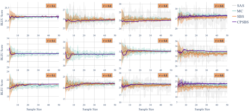
Figure 1: bleu score estimates for three different sentences using estimators for respective decoding methods. $\tau$ indicates scaling temperature; $\tau$ values and sentences are chosen to mimic Kool et al. (2019).

Sum and Sample.

The sum-and-sample estimator Botev et al. (2017); Liu et al. (2019); Kool et al. (2020) is an unbiased estimator that takes as input a deterministically chosen set $Y$ of size $K-1$ and samples an additional $\mathbf{y}^{\prime}$ from the remaining elements, $\mathrm{supp}(p)\setminus Y$, where we obtain the set $Y$ using beam search in our experiments. Formally, the SAS estimator can be written as:

$$G_{\textsc{sas}}\mathrel{\stackrel{{\scriptstyle\textnormal{def}}}{{=}}} \sum_{k=1}^{K-1}p(\mathbf{y}^{(k)})f(\mathbf{y}^{(k)})$$ (30)

$$\quad\quad+\left(1-\sum_{k=1}^{K-1}p(\mathbf{y}^{(k)})\right)f(\mathbf{y}^{\prime})$$

Stochastic Beam Search.

Stochastic beam search Kool et al. (2019, 2020) is a SWOR algorithm likewise built on top of beam search. The algorithm makes use of truncated Gumbel random variables at each iteration, resulting in a sampling design equivalent to performing the Gumbel-top-$k$ trick Vieira (2014) on the distribution $p$. Estimators built using SBS likewise follow the Horvitz–Thompson scheme of Eq. 17; we refer the reader to the original work for inclusion probability computations. They suggest normalizing the estimator by the sum of sample inclusion probabilities to help reduce variance; we therefore likewise perform this normalization in our experiments.

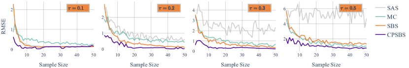
(a) RMSE of bleu score estimator for different temperatures. Results are averaged across several sentences.

(b) RMSE of conditional model entropy estimator for various temperatures. Results are averaged across several sentences. We see a larger bias under both CPSBS and SBS at higher temperatures in these experiments.

Figure 2: RMSE evaluations.

To assess the error of our estimator, we compute its root MSE (RMSE) with respect to a baseline result. While computing the exact value of an expectation is typically infeasible in the sequence model setting, we can average our (unbiased) MC estimator in Eq. 16 over multiple runs to create a good baseline. Specifically, we compute our MC estimator 50 times for a large sample size ($K=200$); variances are reported in App. D.

Probabilistic models for language generation typically have large vocabularies. In this setting, the computation of Eq. 12 is inefficient due to the large number of items in the set that are assigned very small probability under the model. We experiment with truncating this distribution such that the set of possible extensions of a sequence consist only of the highest probability tokens within the core $n$% of probability mass ($0.99$ in our experiments), similar to the process in nucleus sampling Holtzman et al. (2020). We compare this approach to the original algorithm design in App. D and see that empirically, results are virtually unchanged; the following results use this method. We also compare the decoding time of different sampling methods in Fig. 7.

bleu Score Estimation.

bleu Papineni et al. (2002) is a widely used automatic evaluation metric for the quality of machine-generated translations. Estimates of bleu score are used in minimum risk training Shen et al. (2016) and reinforcement learning-based approaches Ranzato et al. (2016) to machine translation. As such, accurate and low-variance estimates are critical for the algorithms’ performance. Formally, we estimate the expected value of $f(\mathbf{y})=\textsc{bleu}(\mathbf{x},\mathbf{y})$, whose dependence on $\mathbf{x}$ we leave implicit, under our NMT model $p$ for reference translation $\mathbf{x}$. For comparison, we use the same sentences and similar annealing temperatures $\tau$ evaluated by Kool et al. (2019). We repeat the sampling 20 times and plot the value and standard deviation (indicated by shaded region) of different estimators in Fig. 1. From Fig. 1, we can see that CPSBS has lower variance than our baseline estimators across all temperatures and data points. Especially in the low temperature setting, our estimator converges rapidly with minor deviation from the exact values even for small sample sizes. Additionally, in Fig. 2(a) we see that the RMSE is typically quite low except at higher temperatures. In such cases, we observe the effects of biasedness, similar to Kool et al. (2019)’s observations.

Conditional Entropy Estimation.

We perform similar experiments for estimates of a model’s conditional entropy, i.e., $f(\mathbf{y})=-\log p(\mathbf{y}\mid\mathbf{x})$, whose dependence on $\mathbf{x}$ we again leave implicit. We show results in Fig. 2(b), with plots of the value in App. D since results are quite similar to Fig. 1. We see further confirmation that our estimator built on CPSBS is generally quite efficient.

5.2 Diverse Sampling

We show how CPSBS can be used as a diverse set sampling design for language generation models. We generate a sample of translations $Y_{T}\sim P$, i.e., according to the CPSBS scheme, where weights are set as $w_{n}=p(\mathbf{y}^{\scaleto{(n)}{6pt}}_{\scaleto{\leq t}{5pt}})/(1-p(\mathbf{y}^{\scaleto{(n)}{6pt}}_{\scaleto{\leq t}{5pt}}))$ at each time step, as recommended in § 3. In Fig. 3, we show the trade-off between minimum, average and maximum sentence-level bleu score (as a quality measure) and $n$-gram diversity, where we define $n$-gram diversity $D$ as the average fraction of unique vs. total $n$-grams for $n=1,2,3,4$ in a sentence:

$$D=\sum_{n=1}^{4}\frac{\#\textrm{unique $n$-grams in $K$ strings}}{\#\textrm{ $n$-grams in $K$ strings}}$$ (31)

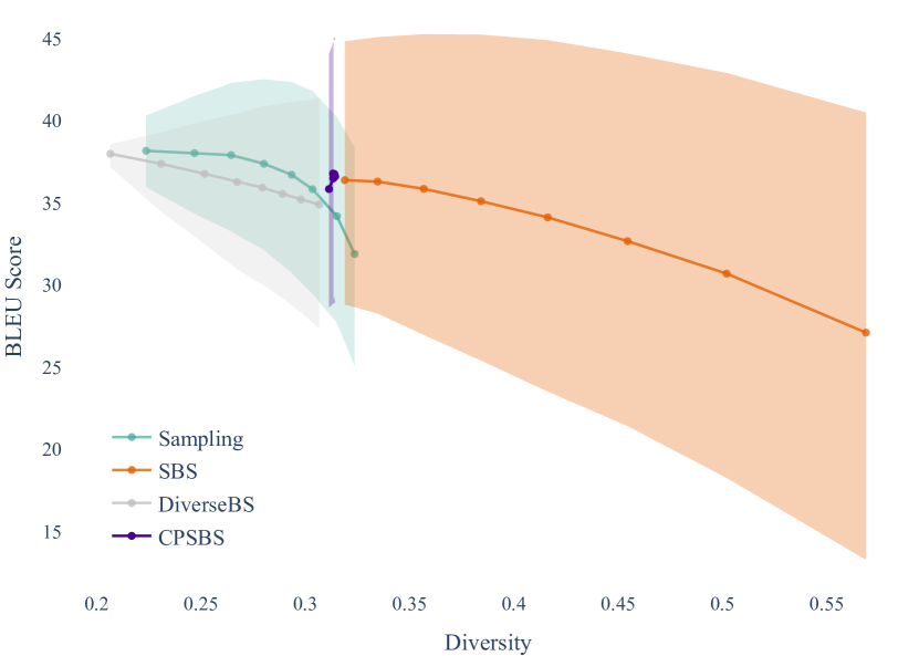
Figure 3: Average ($\pm$ min and max) bleu score versus diversity for sample size $k=5$. Points correspond to different annealing temperatures {0.1, …, 0.8}. Results for $k=10,20$ show very similar trends.

Metrics are averaged across the corpus. We follow the experimental setup of Kool et al. (2019), using the newstest2014 dataset and comparing three different decoding methods: SBS, diverse beam search (DiverseBS; Vijayakumar et al., 2018) and ancestral sampling. As in their experiments, we vary the annealing temperature in the range $\{0.1,0.2,\ldots,0.8\}$ as a means of encouraging diversity; for DiverseBS we instead vary the strength parameter in the same range. Interestingly, we see that temperature has virtually no effect on the diversity of the set of results returned by CPSBS. Despite this artifact, for which the authors have not found a theoretical justification, the set returned by CPSBS is still overall more diverse (position on $x$-axis) than results returned by DiverseBS and reflect better min, max, and average bleu in comparison to random sampling. SBS provides a better spectrum for the diversity and bleu tradeoff; we thus recommend SBS when diverse sets are desired.

6 Conclusion

In this work, we present conditional Poisson stochastic beam search, a sampling-without-replacement strategy for sequence models. Through a simple modification to beam search, we turn this mainstay decoding algorithm into a stochastic process. We derive a low-variance, consistent estimator of inclusion probabilities under this scheme; we then present a general framework for using CPSBS to construct statistical estimators for expectations under sequence models. In our experiments, we observe a reduction in mean square error, and an increase in sample efficiency, when using our estimator in comparison to several baselines, showing the benefits of CPSBS.

Appendix A Conditional Poisson Sampling

Here we provide a brief overview of the sampling design at the core of CPSBS: conditional Poisson sampling. We consider a base set $B$ where $|B|=N$ and we map the elements of $B=\{\mathbf{y}^{(1)},\ldots,\mathbf{y}^{(N)}\}$ to the integers $\{1,\ldots,N\}$. As a warm up, we first consider (unconditional) Poisson sampling, also known as a Bernoulli point process. To sample a subset $Y\subseteq B$, we do as follows: for each element $\mathbf{y}\in B$, we flip a coin where the odds of heads is $w(\mathbf{y})$. Then, we simply take $Y$ to be the subset of elements whose coin flips were heads. However, this sampling scheme clearly does not guarantee a sample of $K$ items, which can cause problems in our application; sampling more than $K$ items would make the stochastic beam search process inefficient while sampling fewer than $K$—or even 0—items may not leave us with a large enough set at the end of our iterative process.

If instead, we condition on the sets always having a prescribed size $K$, i.e., reject samples where $|Y|\neq K$, we arrive at the conditional Poisson process. Formally, the conditional Poisson distribution is defined over $Y\subseteq B$ as follows,

$$Q(Y)\mathrel{\stackrel{{\scriptstyle\textnormal{def}}}{{\propto}}}\begin{cases}\prod_{\mathbf{y}\in Y}w(\mathbf{y})&\textbf{if }|Y|\!=\!K\\ 0&\textbf{otherwise}\end{cases}$$ (32)

By analyzing Eq. 32, we can see that sets with the largest product of weights are the most likely to be sampled; further, this distribution is invariant to rescaling of weights due to the size requirement. This is similar to the conditions under which beam search chooses the set of $K$ largest weight, i.e., highest scoring, elements. Indeed, we note the extreme similarity between Eq. 4 and Eq. 32, the only difference being a dependence on a prior set. However, unlike beam search, sets with a lower weight product now have the possibility of being chosen.

Appendix B Proofs

B.1 Unbiasedness of the Horvitz–Thompson Estimator

Proposition B.1.

Given a SWOR design $Q$ over the set $B=\{1,\dots,N\}$ with inclusion probabilities $\pi(n)$, the Horvitz–Thompson estimator (Eq. 17) gives us an unbiased estimator of $\operatorname*{\mathbb{E}}_{n\sim p}f(n)$, where ${f}:B\rightarrow\mathbb{R}^{d}$ is a function whose expectation under $p$ we seek to approximate.

Proof.

$$\underset{Y\sim Q}{\mathbb{E}}\left[G_{\mathrm{HT}}\right] =\operatorname*{\mathbb{E}}_{Y\sim Q}\sum_{n=1}^{N}\frac{p(n)}{\pi(n)}\,f(n)$$ (33a)

$$=\operatorname*{\mathbb{E}}_{Y\sim Q}\sum_{n\in B}\frac{p(n)}{\pi(n)}\,\mathbbm{1}\{n\in Y\}\,f(n)$$ (33b)

$$=\sum_{n\in B}\frac{p(n)}{\pi(n)}\,f(n)\,\operatorname*{\mathbb{E}}_{Y\sim Q}\mathbbm{1}\{n\in Y\}$$ (33c)

$$=\sum_{n\in B}\frac{p(n)}{\pi(n)}\,f(n)\,\pi(n)$$ (33d)

$$=\sum_{n\in B}p(n)\,f(n)$$ (33e)

$$=\operatorname*{\mathbb{E}}_{n\sim p}f(n)$$ (33f)

∎

B.2 Proofs of Expected Values and Variances of Inclusion Probability Estimators

See 4.1

Proof.

Consider the probability of sampling $\widetilde{Y}_{\!1},\ldots,\widetilde{Y}_{\!T}$ according to $\widetilde{P}$. Algebraic manipulation reveals:

$$\widetilde{P}(\widetilde{Y}_{\!1},\ldots,\widetilde{Y}_{\!T}) =\frac{Q_{t}(\widetilde{Y}_{\!1}\mid Y_{0})}{\pi_{\scaleto{Q_{t}}{5pt}}(\mathbf{y}_{\leq 1}\mid Y_{0})}\cdots\frac{Q_{t}(\widetilde{Y}_{\!T}\mid\widetilde{Y}_{\!T-1})}{\pi_{\scaleto{Q_{t}}{5pt}}(\mathbf{y}_{\leq T}\mid\widetilde{Y}_{\!T-1})}$$ (34a)

$$= \frac{P(\widetilde{Y}_{\!1},\ldots,\widetilde{Y}_{\!T})}{\prod_{t=1}^{T}\pi_{\scaleto{Q_{t}}{5pt}}(\mathbf{y}_{\leq t}\mid\widetilde{Y}_{\!t-1})}\,$$ (34b)

which proves the identity. ∎

See 4.1

Proof.

i) The estimator is easily shown to be unbiased:

$$\operatorname*{\mathbb{E}}\widehat{\pi}^{\scaleto{\textsc{mc}}{3pt}}_{\scaleto{P}{4pt}}(\mathbf{y})\mathrel{\stackrel{{\scriptstyle\textnormal{def}}}{{=}}}\frac{1}{M}\sum_{m=1}^{M}\mathbbm{1}\Big{\{}\mathbf{y}\in Y_{T}^{(m)}\Big{\}}=\pi_{\scaleto{P}{4pt}}(\mathbf{y})$$ (35)

and its variance may be derived as follows:

$$\mathbb{V}\left[\widehat{\pi}^{\scaleto{\textsc{mc}}{3pt}}_{\scaleto{P}{4pt}}(\mathbf{y})\right] \mathrel{\stackrel{{\scriptstyle\textnormal{def}}}{{=}}}\mathbb{V}\left[\frac{1}{M}\sum_{m=1}^{M}\mathbbm{1}\Big{\{}\mathbf{y}\in Y_{T}^{(m)}\Big{\}}\right]$$ (36a)

$$=\frac{1}{M}\mathbb{V}\left[\mathbbm{1}\Big{\{}\mathbf{y}\in Y_{T}^{(m)}\Big{\}}\right]$$ (36b)

$$=\frac{1}{M}\left(\operatorname*{\mathbb{E}}\left(\mathbbm{1}\Big{\{}\mathbf{y}\in Y_{T}^{(m)}\Big{\}}^{2}\right)-\operatorname*{\mathbb{E}}\left(\mathbbm{1}\Big{\{}\mathbf{y}\in Y_{T}^{(m)}\Big{\}}\right)^{2}\right)$$ (36c)

$$=\frac{1}{M}\left(\pi_{\scaleto{P}{4pt}}(\mathbf{y})-\pi_{\scaleto{P}{4pt}}(\mathbf{y})^{2}\right)$$ (36d)

ii) By the strong law of large numbers, we have

$$\lim_{M\rightarrow\infty}\frac{1}{M}\sum_{m=1}^{M}\mathbbm{1}\Big{\{}\mathbf{y}\in Y_{T}^{(m)}\Big{\}}=\pi_{\scaleto{P}{4pt}}(\mathbf{y})$$ (37)

Since $1/x$ is continuous, we may appeal to the continuous mapping theorem to achieve consistency:

$$\lim_{M\rightarrow\infty}\frac{1}{\frac{1}{M}\sum_{m=1}^{M}\mathbbm{1}\Big{\{}\mathbf{y}\in Y_{T}^{(m)}\Big{\}}}=\frac{1}{\lim_{M\rightarrow\infty}\frac{1}{M}\sum_{m=1}^{M}\mathbbm{1}\Big{\{}\mathbf{y}\in Y_{T}^{(m)}\Big{\}}}=\frac{1}{\pi_{\scaleto{P}{4pt}}(\mathbf{y})}$$ (38)

We can compute the asymptotic variance by the delta rule:

$$\mathbb{V}_{\mathrm{a}}\left[\frac{1}{\widehat{\pi}^{\scaleto{\textsc{mc}}{3pt}}_{\scaleto{P}{4pt}}(\mathbf{y})}\right] =\frac{1}{M}\frac{\mathbb{V}\left[\widehat{\pi}^{\scaleto{\textsc{is}}{3pt}}_{\scaleto{P}{4pt}}(\mathbf{y})\right]}{\pi_{\scaleto{P}{4pt}}(\mathbf{y})^{4}}\quad\quad\quad\quad\text{\color[rgb]{.5,.5,.5} (apply the delta rule)}$$ (39a)

$$=\frac{1}{M}\frac{\pi_{\scaleto{P}{4pt}}(\mathbf{y})-\pi_{\scaleto{P}{4pt}}(\mathbf{y})^{2}}{\pi_{\scaleto{P}{4pt}}(\mathbf{y})^{4}}\quad\text{\color[rgb]{.5,.5,.5} (plugging in the variance computed above)}$$ (39b)

$$=\frac{1}{M}\left(\frac{1}{\pi_{\scaleto{P}{4pt}}(\mathbf{y})^{3}}-\frac{1}{\pi_{\scaleto{P}{4pt}}(\mathbf{y})^{2}}\right)$$ (39c)

∎

See 4.2

Proof.

i) We first prove that the estimator of the inclusion probabilities is unbiased through the following manipulation:

$$\operatorname*{\mathbb{E}}\left[\widehat{\pi}^{\scaleto{\textsc{is}}{3pt}}_{\scaleto{P}{4pt}}(\mathbf{y})\right] =\operatorname*{\mathbb{E}}\Bigg{[}\frac{1}{M}\sum_{m=1}^{M}\prod_{t=1}^{T}\pi_{\scaleto{Q_{t}}{5pt}}(\mathbf{y}_{\leq t}\mid\widetilde{Y}_{\!t-1}^{(m)})\Bigg{]}$$ (40a)

$$=\sum_{\widetilde{Y}_{\!1},\ldots,\widetilde{Y}_{\!T}}\widetilde{P}(\widetilde{Y}_{\!1},\ldots,\widetilde{Y}_{\!T})\prod_{t=1}^{T}\pi_{\scaleto{Q_{t}}{5pt}}(\mathbf{y}_{\leq t}\mid\widetilde{Y}_{\!t-1})$$ (40b)

$$=\sum_{\widetilde{Y}_{\!1},\ldots,\widetilde{Y}_{\!T}}\widetilde{P}(\widetilde{Y}_{\!1},\ldots,\widetilde{Y}_{\!T})\frac{P(\widetilde{Y}_{\!1},\ldots,\widetilde{Y}_{\!T})}{P(\widetilde{Y}_{\!1},\ldots,\widetilde{Y}_{\!T})}\prod_{t=1}^{T}\pi_{\scaleto{Q_{t}}{5pt}}(\mathbf{y}_{\leq t}\mid\widetilde{Y}_{\!t-1})$$ (40c)

$$=\sum_{\widetilde{Y}_{\!1},\ldots,\widetilde{Y}_{\!T}}P(\widetilde{Y}_{\!1},\ldots,\widetilde{Y}_{\!T})\frac{\widetilde{P}(\widetilde{Y}_{\!1},\ldots,\widetilde{Y}_{\!T})}{\widetilde{P}(\widetilde{Y}_{\!1},\ldots,\widetilde{Y}_{\!T})}\quad\quad\quad\text{\color[rgb]{.5,.5,.5} {(\lx@cref{creftype~refnum}{lem:decomposition})}}$$ (40d)

$$=\sum_{\widetilde{Y}_{\!1},\ldots,\widetilde{Y}_{\!T}}P(\widetilde{Y}_{\!1},\ldots,\widetilde{Y}_{\!T})$$ (40e)

$$=\sum_{Y_{1},\ldots,Y_{T}}P(Y_{1},\ldots,Y_{T})\,\mathbbm{1}\Big{\{}\mathbf{y}\in Y_{T}\Big{\}}\quad\quad\quad\text{\color[rgb]{.5,.5,.5} {(definition of $\widetilde{Y}_{\!T}$)}}$$ (40f)

$$=\pi_{\scaleto{P}{4pt}}(\mathbf{y})$$ (40g)

ii) To show consistency, we appeal to the strong law of large number and the continuous mapping theorem. By the strong law of large numbers, we have that

$$\lim_{M\rightarrow\infty}\frac{1}{M}\sum_{m=1}^{M}\prod_{t=1}^{T}\pi_{\scaleto{Q_{t}}{5pt}}(\mathbf{y}_{\leq t}\mid\widetilde{Y}_{\!t-1}^{(m)})=\pi_{\scaleto{P}{4pt}}(\mathbf{y})$$ (41)

Since $1/x$ is continuous, we have

$$\lim_{M\rightarrow\infty}\frac{1}{\frac{1}{M}\sum_{m=1}^{M}\prod_{t=1}^{T}\pi_{\scaleto{Q_{t}}{5pt}}(\mathbf{y}_{\leq t}\mid\widetilde{Y}_{\!t-1}^{(m)})} =\frac{1}{\lim_{M\rightarrow\infty}\frac{1}{M}\sum_{m=1}^{M}\prod_{t=1}^{T}\pi_{\scaleto{Q_{t}}{5pt}}(\mathbf{y}_{\leq t}\mid\widetilde{Y}_{\!t-1}^{(m)})}$$

$$=\frac{1}{\pi_{\scaleto{P}{4pt}}(\mathbf{y})}$$ (42a)

which shows consistency. Now, we derive a bound on the asymptotic variance of the inverse inclusion probabilities. First, suppose that

$$\frac{\prod_{t=1}^{T}\pi_{\scaleto{Q_{t}}{5pt}}(\mathbf{y}_{\leq t}\mid\widetilde{Y}_{\!t-1})}{\pi_{\scaleto{P}{4pt}}(\mathbf{y})}\leq r,\quad\forall\,\widetilde{Y}_{\!1},\ldots,\widetilde{Y}_{\!T}$$ (43)

We start with the variance of importance sampling. This is a standard result Rubinstein and Kroese (2016). Then we proceed with algebraic manipulation integrating the assumption above:

$$\sum_{\widetilde{Y}_{\!1},\ldots,\widetilde{Y}_{\!T}} \frac{\mathbbm{1}\Big{\{}\mathbf{y}\in\widetilde{Y}_{\!T}\Big{\}}^{2}P(\widetilde{Y}_{\!1},\ldots,\widetilde{Y}_{\!T})^{2}}{\widetilde{P}(\widetilde{Y}_{\!1},\ldots,\widetilde{Y}_{\!T})}-\pi_{\scaleto{P}{4pt}}(\mathbf{y})^{2}$$ (44a)

$$=\sum_{\widetilde{Y}_{\!1},\ldots,\widetilde{Y}_{\!T}}P(\widetilde{Y}_{\!1},\ldots,\widetilde{Y}_{\!T})\prod_{t=1}^{T}\pi_{\scaleto{Q_{t}}{5pt}}(\mathbf{y}_{\leq t}\mid\widetilde{Y}_{\!t-1})-\pi_{\scaleto{P}{4pt}}(\mathbf{y})^{2}$$ (44b)

$$\leq\sum_{\widetilde{Y}_{\!1},\ldots,\widetilde{Y}_{\!T}}P(\widetilde{Y}_{\!1},\ldots,\widetilde{Y}_{\!T})\pi_{\scaleto{P}{4pt}}(\mathbf{y})r-\pi_{\scaleto{P}{4pt}}(\mathbf{y})^{2}$$ (44c)

$$=\pi_{\scaleto{P}{4pt}}(\mathbf{y})\pi_{\scaleto{P}{4pt}}(\mathbf{y})r-\pi_{\scaleto{P}{4pt}}(\mathbf{y})^{2}$$ (44d)

$$=\pi_{\scaleto{P}{4pt}}(\mathbf{y})^{2}r-\pi_{\scaleto{P}{4pt}}(\mathbf{y})^{2}$$ (44e)

$$=(r-1)\pi_{\scaleto{P}{4pt}}(\mathbf{y})^{2}$$ (44f)

We can compute the asymptotic variance by the delta rule:

$$\mathbb{V}_{\mathrm{a}}\left[\frac{1}{\widehat{\pi}^{\scaleto{\textsc{is}}{3pt}}_{\scaleto{P}{4pt}}(\mathbf{y})}\right] =\frac{1}{M}\frac{\mathbb{V}\left[\widehat{\pi}^{\scaleto{\textsc{is}}{3pt}}_{\scaleto{P}{4pt}}(\mathbf{y})\right]}{\pi_{\scaleto{P}{4pt}}(\mathbf{y})^{4}}\quad\quad\text{\color[rgb]{.5,.5,.5} (apply the delta rule)}$$ (45a)

$$\leq\frac{1}{M}\frac{(r-1)\pi_{\scaleto{P}{4pt}}(\mathbf{y})^{2}}{\pi_{\scaleto{P}{4pt}}(\mathbf{y})^{4}}\quad\text{\color[rgb]{.5,.5,.5} (plugging in the above bound)}$$ (45b)

$$=\frac{1}{M}\frac{(r-1)}{\pi_{\scaleto{P}{4pt}}(\mathbf{y})^{2}}$$ (45c)

which proves the result.

∎

Appendix C Pseudocode

Input: $K$: Size of subset
          $w_{1},\ldots,w_{N}$: weights for each element of the base set
Output: $W$: elementary symmetric polynomials of $w_{1},\ldots,w_{N}$; $Z=W_{N,K}$

1:$W\leftarrow\boldsymbol{0}^{(K+1)\times(N+1)}$

2:$W_{0,:}=0;\,W_{:,0}=1$

3:for $n=1,\dots,N$ :

4:   for $k=1,\dots,K$ :

5:      $W_{n,k}\leftarrow W_{n-1,k}+w_{n}W_{n-1,k-1}$    

6:return $W$

Algorithm 1 Dynamic program algorithm for $\mathrm{Z}$

Input: $K$: Size of subset
          $w_{1},\ldots,w_{N}$: weights for each element of the base set

1:Run Alg. 1 to compute $W$

2: $\triangleright$ The code below was derived by manually apply algorithmic differentiation Bücker et al. (2006) to Alg. 1.

3:$\accentset{\mbox{.}}{W}\leftarrow\boldsymbol{0}^{(K+1)\times(N+1)}$ $\triangleright$ Initialize adjoints

4:$\accentset{\mbox{.}}{w}\leftarrow\boldsymbol{0}^{N}$

5:$\accentset{\mbox{.}}{W}_{N,K}=1$ $\triangleright$ Initialize output value to $1$

6:for $n=N,\ldots,1$ :

7:   for $k=K,\ldots,1$ :

8:      $\accentset{\mbox{.}}{w}_{n}\ \texttt{+=}\ \accentset{\mbox{.}}{W}_{n,k}\,W_{n-1,k-1}$

9:      $\accentset{\mbox{.}}{W}_{n-1,k-1}\ \texttt{+=}\ \accentset{\mbox{.}}{W}_{n,k}\,w_{n}$

10:      $\accentset{\mbox{.}}{W}_{n-1,k}\ \texttt{+=}\ \accentset{\mbox{.}}{W}_{n,k}$    

11: $\triangleright$ Apply Eq. 24

12:$\pi\leftarrow\boldsymbol{0}^{N}$

13:for $n=1\ldots N$ :

14:   $\pi_{n}\leftarrow\frac{w_{n}}{\mathrm{Z}}\accentset{\mbox{.}}{w}_{n}$ return $\pi$

Algorithm 2 Dynamic program for calculating inclusion probabilities $\pi$

Appendix D Experimental Setup and Additional Results

We use a Transformer-based model trained according to Ott et al. (2018b) on the WMT’14 English-French dataset. We use the pre-trained model checkpoints made available by fairseq. Data preprocessing steps, model hyperparameters and baseline performances can be found in the original work and on the fairseq website. All evaluations are performed on the wmt14.v2.en-fr.newstest2014 version of the newstest data set. We show additional results using the setup in § 5 in Figs. 4, 5 and 6. We provide an empirical runtime analysis in Fig. 7. Table 2 shows the variance of baseline estimator value for the three sentences used in RMSE experiments.

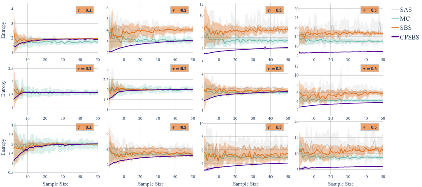
Figure 4: Entropy estimates for three different sentences using estimators for respective decoding methods. $\tau$ indicates scaling temperature. Values are chosen to mimic Kool et al. (2019).

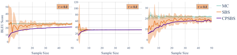
Figure 5: bleu score estimates using unnormalized versions of SBS and CPSBS estimators.

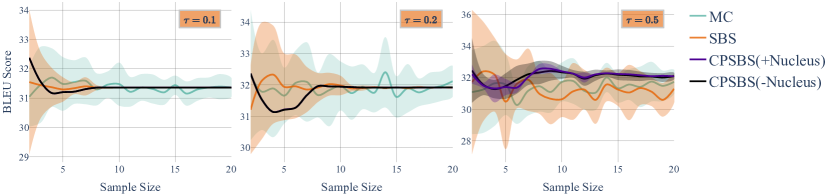
Figure 6: bleu score estimates for CPSBS both with and without truncation of the sampling distribution. We see that our estimator with truncation provides virtually the same results.

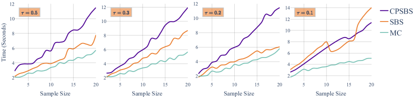
Figure 7: A comparison between decoding time of different sampling methods. The y-axis shows the average decoding time of the three sentences as before. The x-axis shows the number of samples taken for each sentence. All methods are tested on CPU.

	bleu Estimator					Entropy Estimator
	Temperature					Temperature
	0.1	0.2	0.3	0.5		0.1	0.2	0.3	0.5
Sentence# 1500	0.00	0.00	0.03	0.08		0.00	0.01	0.07	0.10
Sentence# 2000	0.01	0.04	0.04	0.08		0.00	0.00	0.00	0.02
Sentence# 2500	0.07	0.09	0.25	0.84		0.00	0.01	0.03	0.04

Table 2: Variance of baseline estimator (MC for $k=200$ in 50 iterations) for the three sentences.

References

- Aires (1999) Nibia Aires. 1999. Algorithms to find exact inclusion probabilities for conditional Poisson sampling and Pareto ps sampling designs. Methodology and Computing in Applied Probability, 1(4):457–469.
- Bickel and Docksum (2015) Peter J. Bickel and Kjell A. Docksum. 2015. Mathematical Statistics: Basic ideas and Selected Topics. CRC Press.
- Bojar et al. (2014) Ondřej Bojar, Christian Buck, Christian Federmann, Barry Haddow, Philipp Koehn, Johannes Leveling, Christof Monz, Pavel Pecina, Matt Post, Herve Saint-Amand, Radu Soricut, Lucia Specia, and Aleš Tamchyna. 2014. Findings of the 2014 workshop on statistical machine translation. In Proceedings of the Ninth Workshop on Statistical Machine Translation, pages 12–58, Baltimore, Maryland, USA. Association for Computational Linguistics.
- Bondesson et al. (2006) Lennart Bondesson, Imbi Traat, and Anders Lundqvist. 2006. Pareto sampling versus Sampford and conditional Poisson sampling. Scandinavian Journal of Statistics, 33(4):699–720.
- Botev et al. (2017) Aleksandar Botev, Bowen Zheng, and David Barber. 2017. Complementary sum sampling for likelihood approximation in large scale classification. In Proceedings of the International Conference on Artificial Intelligence and Statistics.
- Bücker et al. (2006) Martin Bücker, George Corliss, Paul Hovland, Uwe Naumann, and Boyana Norris. 2006. Automatic Differentiation: Applications, Theory, and Implementations (Lecture Notes in Computational Science and Engineering). Springer-Verlag, Berlin, Heidelberg.
- Edunov et al. (2018) Sergey Edunov, Myle Ott, Michael Auli, and David Grangier. 2018. Understanding back-translation at scale. In Proceedings of the 2018 Conference on Empirical Methods in Natural Language Processing, pages 489–500, Brussels, Belgium. Association for Computational Linguistics.
- Eikema and Aziz (2020) Bryan Eikema and Wilker Aziz. 2020. Is MAP decoding all you need? The inadequacy of the mode in neural machine translation. In Proceedings of the 28th International Conference on Computational Linguistics, pages 4506–4520, Barcelona, Spain (Online). International Committee on Computational Linguistics.
- Grafström (2009) Anton Grafström. 2009. Non-rejective implementations of the Sampford sampling design. Journal of Statistical Planning and Inference, 139(6):2111–2114.
- Hájek (1981) J. Hájek. 1981. Sampling from a Finite Population. Statistics Series. Marcel Dekker.
- Hájek (1964) Jaroslav Hájek. 1964. Asymptotic theory of rejective sampling with varying probabilities from a finite population. Annals of Mathematical Statistics, 35(4):1491–1523.
- Holtzman et al. (2020) Ari Holtzman, Jan Buys, Li Du, Maxwell Forbes, and Yejin Choi. 2020. The curious case of neural text degeneration. In Proceedings of the 7th International Conference on Learning Representations.
- Horvitz and Thompson (1952) D. G. Horvitz and D. J. Thompson. 1952. A generalization of sampling without replacement from a finite universe. Journal of the American Statistical Association, 47(260):663–685.
- Kool et al. (2019) Wouter Kool, Herke Van Hoof, and Max Welling. 2019. Stochastic beams and where to find them: The Gumbel-top- trick for sampling sequences without replacement. In Proceedings of the 36th International Conference on Machine Learning.
- Kool et al. (2020) Wouter Kool, Herke van Hoof, and Max Welling. 2020. Estimating gradients for discrete random variables by sampling without replacement. In Proceedings of the 8th International Conference on Learning Representations.
-
Kulesza and Taskar (2012)
Alex Kulesza and Ben Taskar. 2012.
Determinantal point
processes for machine learning.
Foundations and Trends