Abstract

We reemphasize the strong dependence of the branching ratios $\mathcal{B}(K^{+}\to\pi^{+}\nu\bar{\nu})$ and $\mathcal{B}(K_{L}\to\pi^{0}\nu\bar{\nu})$ on $|V_{cb}|$ that is stronger than in rare $B$ decays, in particular for $K_{L}\to\pi^{0}\nu\bar{\nu}$. Thereby the persistent tension between inclusive and exclusive determinations of $|V_{cb}|$ weakens the power of these theoretically clean decays in the search for new physics (NP). We demonstrate how this uncertainty can be practically removed by considering within the SM suitable ratios of the two branching ratios between each other and with other observables like the branching ratios for $K_{S}\to\mu^{+}\mu^{-}$, $B_{s,d}\to\mu^{+}\mu^{-}$ and $B\to K(K^{*})\nu\bar{\nu}$. We use as basic CKM parameters $V_{us}$, $|V_{cb}|$ and the angles $\beta$ and $\gamma$ in the unitarity triangle (UT) with the latter two determined through the measurements of tree-level $B$ decays. This avoids the use of the problematic $|V_{ub}|$. A ratio involving $\mathcal{B}(K^{+}\to\pi^{+}\nu\bar{\nu})$ and $\overline{\mathcal{B}}(B_{s}\to\mu^{+}\mu^{-})$ while being $|V_{cb}|$-independent exhibits sizable dependence on the angle $\gamma$. It should be of interest for several experimental groups in the coming years. We point out that the $|V_{cb}|$-independent ratio of $\mathcal{B}(B^{+}\to K^{+}\nu\bar{\nu})$ and $\overline{\mathcal{B}}(B_{s}\to\mu^{+}\mu^{-})$ from Belle II and LHCb signals a $1.8\sigma$ tension with its SM value. As a complementary test of the Standard Model we propose to extract $|V_{cb}|$ from different observables as a function of $\beta$ and $\gamma$. We illustrate this with $\varepsilon_{K}$, $\Delta M_{d}$ and $\Delta M_{s}$ finding tensions between these three determinations of $|V_{cb}|$ within the SM. We point out that from $\Delta M_{s}$ and $S_{\psi K_{S}}$ alone one finds $|V_{cb}|=41.8(6)\times 10^{-3}$ and $|V_{ub}|=3.65(12)\times 10^{-3}$. We stress the importance of a precise measurement of $\gamma$. Assuming no NP in $|\varepsilon_{K}|$ and $S_{\psi K_{S}}$ we determine independently of $|V_{cb}|$ and $\gamma$: $\mathcal{B}(K^{+}\rightarrow\pi^{+}\nu\bar{\nu})_{\text{SM}}=(8.60\pm 0.42)\times 10^{-11}$ and $\mathcal{B}(K_{L}\rightarrow\pi^{0}\nu\bar{\nu})_{\text{SM}}=(2.94\pm 0.15)\times 10^{-11}$ with only CKM uncertainty coming from $\beta$, that is already precisely known. These are the most precise determinations to date. Assuming no NP in $\Delta M_{s,d}$ allows to obtain analogous results for all $B$ decay branching ratios considered in our paper without any CKM uncertainties.

1 Introduction

The rare decays $K^{+}\rightarrow\pi^{+}\nu\bar{\nu}$ and $K_{L}\rightarrow\pi^{0}\nu\bar{\nu}$ played already for three decades an important role in the tests of the Standard Model (SM) and of its various extensions [1, 2]. This is due to their theoretical cleanness and GIM suppression of their branching ratios within the SM implying strong sensitivity to new physics (NP).

On the experimental side the most recent result for $K^{+}\rightarrow\pi^{+}\nu\bar{\nu}$ from NA62 [3] and the $90\%$ C.L. upper bound on $K_{L}\rightarrow\pi^{0}\nu\bar{\nu}$ from KOTO [4] read respectively

$$\mathcal{B}(K^{+}\rightarrow\pi^{+}\nu\bar{\nu})_{\text{exp}}=(10.6^{+4.0}_{-3.5}\pm 0.9)\times 10^{-11}\,,\qquad\mathcal{B}(K_{L}\rightarrow\pi^{0}\nu\bar{\nu})_{\text{exp}}\leq 3.0\times 10^{-9}\,$$ (1)

and are to be compared with the SM predictions of 2015 [5] that are frequently quoted in the literature

$$\mathcal{B}(K^{+}\rightarrow\pi^{+}\nu\bar{\nu})_{\text{SM}}=(8.4\pm 1.0)\times 10^{-11}\,,\qquad\mathcal{B}(K_{L}\rightarrow\pi^{0}\nu\bar{\nu})_{\text{SM}}=(3.4\pm 0.6)\times 10^{-11}\,.$$ (2)

On the other hand the most recent updated predictions for both branching ratios from [7] read

$$\mathcal{B}(K^{+}\rightarrow\pi^{+}\nu\bar{\nu})_{\text{SM}}=(7.7\pm 0.6)\times 10^{-11}\,,\qquad\mathcal{B}(K_{L}\rightarrow\pi^{0}\nu\bar{\nu})_{\text{SM}}=(2.6\pm 0.3)\times 10^{-11}\,.$$ (3)

They are on the one hand significantly lower than the values in (2) and on the other hand are much more accurate.

However, the inspection of the plots in [5] and their updated versions in Fig. 2 of the present paper demonstrate very clearly

• strong dependence of $\mathcal{B}(K^{+}\rightarrow\pi^{+}\nu\bar{\nu})_{\text{SM}}$ on $|V_{cb}|$ and on the angle $\gamma$ in the unitarity triangle (UT), although only a weak dependence on the angle $\beta$,

• strong dependence of $\mathcal{B}(K_{L}\rightarrow\pi^{0}\nu\bar{\nu})_{\text{SM}}$ on $|V_{cb}|$ and the angle $\beta$ in the UT but also significant dependence on $\gamma$.

To obtain the result in (3) the authors of [7] used the values of the CKM parameters from the CKMfitter adopted by PDG [8]. In particular the value of $|V_{cb}|$ corresponding to (3), $|V_{cb}|=(40.5\pm 0.8)\cdot 10^{-3}$, is in the ballpark of exclusive determinations of $|V_{cb}|$, as for example from $B\to D\ell\bar{\nu}$ [9]. Had the authors of [7] used the inclusive determination of $|V_{cb}|$, that is the value $|V_{cb}|_{B\to X_{c}}=(42.16\pm 0.50)\cdot 10^{-3}$ [10], close to the values obtained by Utfitter in their global analysis, they would find significantly higher branching ratio. This is evident from Fig. 2, where the values of branching ratios for $K^{+}\rightarrow\pi^{+}\nu\bar{\nu}$ and $K_{L}\rightarrow\pi^{0}\nu\bar{\nu}$ have been plotted as functions of $|V_{cb}|$ for different values of $\gamma$ and $\beta$. On the other hand the most recent exclusive value of $|V_{cb}|$ from FLAG reads $|V_{cb}|=(39.48\pm 0.68)\cdot 10^{-3}$ [11] which would imply even lower values for branching ratios than given in (3).

This uncertainty in $|V_{cb}|$ is annoying in view of the very small theoretical uncertainties in these two decays, with QCD corrections known at NLO [12, 13, 14, 15] and NNLO level [16, 17, 18] and electroweak corrections at the NLO level [19, 20]. Moreover isospin breaking effects and non-perturbative effects have been considered in [21, 22] and further improvements are expected from lattice gauge theories [23].

It should also be emphasized that as the dominant CKM factor in rare Kaon decays $V_{ts}^{*}V_{td}$ grows with $|V_{cb}|$ like $|V_{cb}|^{2}$, the branching ratio for $K_{L}\rightarrow\pi^{0}\nu\bar{\nu}$ grows with $|V_{cb}|$ like $|V_{cb}|^{4}$ to be compared with $|V_{cb}|^{2}$ in the case of $B_{s}\to\mu^{+}\mu^{-}$, where $V_{td}$ is replaced by $V_{tb}\approx 1$. For $K^{+}\rightarrow\pi^{+}\nu\bar{\nu}$ this dependence is weaker due to the presence of significant charm contribution but still stronger than for $B_{s}\to\mu^{+}\mu^{-}$. Also the short distance contribution to the $K_{S}\to\mu^{+}\mu^{-}$ branching ratio grows like $|V_{cb}|^{4}$ and the $|V_{cb}|$ dependence in the parameter $\varepsilon_{K}$, similar to $K^{+}\rightarrow\pi^{+}\nu\bar{\nu}$, although weaker than $|V_{cb}|^{4}$ due to the presence of charm contribution, is also stronger than in $B_{s}\to\mu^{+}\mu^{-}$.

These strong parametric dependences on $|V_{cb}|$ in $K_{S}\to\mu^{+}\mu^{-}$ and $\varepsilon_{K}$, combined with the uncertainty in $|V_{cb}|$, are also unfortunate because of the recent progress promoting both to precision observables. Indeed

• it has been demonstrated in [24] that the short distance contribution to the $K_{S}\to\mu^{+}\mu^{-}$ branching ratio can be extracted from data offering us still another precision observable subject only to the parametric uncertainties stressed above.

• the significant QCD uncertainty from pure charm contribution to $\varepsilon_{K}$ has been practically removed in [25] through a clever but simple trick by using CKM unitarity differently than done until now in the literature. Moreover, the two-loop electroweak effects on the top contribution have been found to decrease $\varepsilon_{K}$ by less than $1\%$ [26]. These reductions of theoretical uncertainties in $\varepsilon_{K}$ will play a significant role in our analysis. Therefore this new improvement in [25] should be incorporated in any global analysis like the ones used in the PDG.

So far we discussed only the $|V_{cb}|$ dependence but the $|V_{ub}|$ parameter is also relevant. In view of the tensions between exclusive and inclusive determinations of $|V_{ub}|$ that are also sizable [27], we will, following [28], use as four basic CKM parameters

$$\boxed{\lambda=|V_{us}|,\qquad|V_{cb}|,\qquad\beta,\qquad\gamma}$$ (4)

with $\beta$ and $\gamma$ being two angles in the UT, shown in Fig. 1. Their determination from mixing induced CP-asymmetries in tree-level $B$ decays and using other tree-level strategies is presently theoretically cleaner than the determination of $|V_{ub}|$. As demonstrated in [29] the determination of the apex of the UT, given as seen in Fig. 1 by $(\bar{\rho},\bar{\eta})$, by means of the measurements of $\beta$ and $\gamma$ in tree-level $B$ decays is very efficient. A recent review of such determinations of $\beta$ and $\gamma$ can be found in Chapter 8 of [2]. See also [30, 31].

Recently, following the proposal in [32], it has been demonstrated in [33] that considering the ratio of the $B_{s}\to\mu^{+}\mu^{-}$ branching ratio to $\Delta M_{s}$ the parametric uncertainty in $B_{s}\to\mu^{+}\mu^{-}$ due to $|V_{cb}|$ could be totally eliminated allowing confidently to determine possible tension for this ratio between its SM estimate and the data.

We would like to emphasize that in the case of lepton flavour violation and electric dipole moments, where the SM estimates are by orders of magnitude below the present experimental upper bounds, such parametric uncertainties as the one due to $|V_{cb}|$ in rare decays of mesons are presently irrelevant. But in the case of $B_{s}\to\mu^{+}\mu^{-}$ and $K^{+}\rightarrow\pi^{+}\nu\bar{\nu}$ the room left for NP is respectively below $30\%$ and $100\%$ of the SM value and any reduction of parametric uncertainties is important. The case of $K_{L}\rightarrow\pi^{0}\nu\bar{\nu}$ and $K_{S}\to\mu^{+}\mu^{-}$, where the experimental upper bounds are still by at least two orders above the SM expectations, is different. But it is expected that in this decade the branching ratios for these decays will be measured and it is useful to be prepared for such measurements already now. The last statement applies also to $B\to K(K^{*})\nu\bar{\nu}$ and $B_{d}\to\mu^{+}\mu^{-}$ which will play important roles in flavour physics in the coming years.

The main goal of the present paper is the generalization of the strategy in [32, 33] to the theoretically cleanest rare Kaon and $B$-meson decays including also the parameter $\varepsilon_{K}$ which through the progress made in [25] has been promoted within the SM to the class of precision observables. Also the mass differences $\Delta M_{s,d}$ will play a role in these strategies. In doing this we benefited from previous analyses, like the ones in [34, 35, 36, 29, 5, 37, 28]. However, our paper should not be considered as an update of these strategies which would be useful in itself. In particular, in contrast to [37, 28], where the detailed dependence of various observables on $|V_{cb}|$ has been investigated, our goal here is to eliminate this dependence by taking suitable ratios of various observables and in the spirit of [32, 33] to develop strategies for finding footprints of NP in several observables independently of the value of $|V_{cb}|$.

Once the $|V_{cb}|$ dependence is eliminated, the $|V_{cb}|$-independent correlations between various observables depend on only three remaining parameters in (4). But the dependence on $|V_{us}|$ is negligible, the angle $\beta$ is already known from $S_{\psi K_{S}}$ asymmetry with respectable precision and there is a significant progress by the LHCb collaboration on the determination of $\gamma$ from tree-level strategies [38]:

$$\boxed{\beta=(22.2\pm 0.7)^{\circ},\qquad\gamma=(65.4^{+3.8}_{-4.2})^{\circ}\,.}$$ (5)

Moreover, in the coming years the determination of $\gamma$ by the LHCb and Belle II should be significantly improved so that precision tests of the SM using our strategies will be possible.

Now comes an important issue that we would like to emphasize. One could ask the question whether such clean tests of the SM could be accomplished by performing a global analysis of several processes as done in the standard analyses of the UT or the recent global fits testing the violation of lepton flavour universality. Of course such a global analysis may reveal any potential tension by lowering the goodness of the SM fit. However, a clear-cut insight into the origin of tensions is not so easily obtainable. Indeed such analyses involve usually CKM uncertainties, in particular the one from $|V_{cb}|$, and also hadronic uncertainties present in other processes that are larger than the ones in $K^{+}\rightarrow\pi^{+}\nu\bar{\nu}$, $K_{L}\rightarrow\pi^{0}\nu\bar{\nu}$, $K_{S}\to\mu^{+}\mu^{-}$, $B_{s,d}\to\mu^{+}\mu^{-}$, $B\to K(K^{*})\nu\bar{\nu}$, $\Delta M_{d,s}$ and $\varepsilon_{K}$. Moreover, NP could enter many observables used in such global fits and the transparent identification of the impact of NP on a given observable is a challenge. On the contrary, in the proposed strategies that involve ratios of observables, these uncertainties, in particular the one from $|V_{cb}|$, cancel out except for the bag factors and weak decay constants in $\varepsilon_{K}$ and $\Delta M_{d,s}$, which are already precisely known from LQCD and importantly their values do not depend on NP parameters. In this manner concentrating just on the listed decays allows us to test the SM independently of the value of $|V_{cb}|$. These ratios could turn out to be smoking guns of NP.

However, the ratios of branching ratios are not as interesting as branching ratios themselves. Fortunately our strategy allows to determine the latter in a $|V_{cb}|$-independent manner by using solely

$$\boxed{|\varepsilon_{K}|,\qquad S_{\psi K_{S}},\qquad\Delta M_{s},\qquad\Delta M_{d}\,.}$$ (6)

This strategy differs from usual strategies in that not tree-level decays but loop suppressed transitions are used to determine CKM parameters. But within the SM this strategy is legitimate and as the experimental data and theory for these observables, including both perturbative and non-perturbative QCD effects, have smaller uncertainties than tree-level decays one arrives at rather accurate predictions for rare decay branching ratios which is presently impossible otherwise.

In this context we would like to comment on a recent analysis in [39] on a determination of $|V_{cb}|$ and $|V_{ub}|$ from loop processes alone, rare decays and quark mixing, by assuming no NP contributions to these observables. While this analysis is in fact the generalization of one of the strategies suggested in [5] to include additional processes and to perform a global fit, our present strategy in using the observables in (6) differs from the ones in [5] and [39] in the following manner.

We do not assume that NP is absent simultaneously in all four observables in (6) because of some tensions between determinations of $|V_{cb}|$ through these observables which we will identify in Section 3. Therefore, to obtain SM predictions for rare Kaon decays we only assume the absence of NP in $\varepsilon_{K}$ and $S_{\psi K_{S}}$. To obtain predictions for $B_{s}\to\mu^{+}\mu^{-}$ and $B_{d}\to\mu^{+}\mu^{-}$ we assume, following [32], the absence of NP in $\Delta M_{s}$ and $\Delta M_{d}$, respectively but not simultaneously. In our view this strategy for finding SM predictions is presently more powerful than any global fit which would include decays like $B\to K\mu^{+}\mu^{-}$, $B\to K^{*}\mu^{+}\mu^{-}$ and $B_{s}\to\phi\mu^{+}\mu^{-}$ that exhibit significant contributions from NP.

In fact, our strategy allows us to obtain one of the most important results of our paper: the most precise determination of the $K^{+}\rightarrow\pi^{+}\nu\bar{\nu}$ and $K_{L}\rightarrow\pi^{0}\nu\bar{\nu}$ branching ratios within the SM to date. From $\varepsilon_{K}$ and $S_{\psi K_{S}}$ alone with $60^{\circ}\leq\gamma\leq 75^{\circ}$ we find

$$\boxed{\mathcal{B}(K^{+}\rightarrow\pi^{+}\nu\bar{\nu})_{\text{SM}}={(8.60\pm 0.42)}\times 10^{-11}\,,\quad\mathcal{B}(K_{L}\rightarrow\pi^{0}\nu\bar{\nu})_{\text{SM}}={(2.94\pm 0.15)}\times 10^{-11}\,,}$$ (7)

which supersede the usually quoted values in (2). In fact in the first case the error is reduced by a factor of $2.4$ and in the second case by a factor of $4$. The agreement of the central value for $K^{+}\rightarrow\pi^{+}\nu\bar{\nu}$ with the one in (2) is accidental. The latter result was obtained by using some average values of $|V_{cb}|$ and $|V_{ub}|$ from tree-level determinations and the 2015 value of $\gamma$ that was significantly higher than the one in (5).

Most importantly these results are independent of the value of $|V_{cb}|$ and the error includes the full variation of $\gamma$ in the range even larger than the usual CKM global fits. The crucial idea behind it is the elimination of the $|V_{cb}|$ dependence of both branching ratios with the help of $\varepsilon_{K}$ with an additional bonus, very strong suppression of the $\gamma$ dependence of both branching ratios so that the only relevant CKM uncertainty included in the error comes from $\beta$ that is already precisely known from the measurements of $S_{\psi K_{S}}$. Indeed these results are more accurate than the ones in (2) and (3) and are not subject to any uncertainties related to $|V_{cb}|$ and $|V_{ub}|$. As the $|V_{cb}|$ dependence of the $K_{L}\rightarrow\pi^{0}\nu\bar{\nu}$ branching ratio is stronger than in the $K^{+}\rightarrow\pi^{+}\nu\bar{\nu}$ case, the reduction of the error is larger. Moreover the future measurement of $\gamma$ will only have a minor impact on them. Further decrease of the errors can only be achieved by a more precise determination of $\beta$ and the reduction of the remaining non-perturbative uncertainties in $K^{+}\rightarrow\pi^{+}\nu\bar{\nu}$ ($P_{c}$) and in $\varepsilon_{K}$ ($\kappa_{\epsilon}$).

Proceeding in this manner and using the results of [33] together with very precise experimental values for $\Delta M_{s,d}$ we find

$$\boxed{\overline{\mathcal{B}}(B_{s}\to\mu^{+}\mu^{-})_{\rm SM}=(3.62^{+0.15}_{-0.10})\times 10^{-9},\qquad\mathcal{B}(B_{d}\to\mu^{+}\mu^{-})_{\rm SM}=(0.99^{+0.05}_{-0.03})\ \times 10^{-10},}$$ (8)

which are in the ballpark of the SM values quoted in the literature [12, 15, 40, 41, 42, 43] but have the advantage of being independent of the value of $|V_{cb}|$ and in fact of any CKM parameter. Similar to (7) the results in (8) are most accurate to date.

As already pointed out in [33] the ratio of $\overline{\mathcal{B}}(B_{s}\to\mu^{+}\mu^{-})$ to $\Delta M_{s}$ is in $2.2\sigma$ tension with the data. Assuming $\Delta M_{s}$ is SM-like and using for it the experimental data exhibits in (8) this tension explicitly when compared with the experimental data in (46).

The outline of our paper is as follows. In Section 2 we recall the formulae for the sides and the apex of the UT given in terms of the set (4). Subsequently we present a number of very accurate formulae for rare $K$ and $B$ decays considered by us in terms of this set of parameters. They in turn allow us to derive in a straightforward manner a number of accurate relations between various observables that are independent of $|V_{cb}|$ and often exhibit very weak dependence on the remaining parameters. These relations are valid only in the SM and their violation would signal NP at work.

In Section 3, as a complementary test of the SM, that in contrast to the usual UT analyses exhibits the $|V_{cb}|$ dependence, we propose to extract $|V_{cb}|$ from different processes as a function of $\beta$ and $\gamma$. This in turn allows the determination of $|V_{ub}|$ as a function of these two UT angles. We illustrate this with $\varepsilon_{K}$, $\Delta M_{d}$ and $\Delta M_{s}$. This in turn using $|V_{cb}|$ from $\varepsilon_{K}$ allows to calculate $K^{+}\rightarrow\pi^{+}\nu\bar{\nu}$ and $K_{L}\rightarrow\pi^{0}\nu\bar{\nu}$ branching ratios as functions of $\gamma$ and $\beta$ without any explicit $|V_{cb}|$ and $|V_{ub}|$ dependences. As the $\gamma$ dependence is very weak, imposing the constraint on $\beta$ from $S_{\psi K_{S}}$ we obtain, as seen in (7), the most precise estimate of both branching ratios to date.

For $B_{s,d}$ decays analogous use of $\Delta M_{s,d}$ eliminates the CKM dependence from branching ratios [32, 33] leading to the result in (8). Inserting the results in (7) and (8) into the $|V_{cb}|$-independent ratios involving the remaining three decays, $K_{S}\to\mu^{+}\mu^{-}$, $B^{+}\to K^{+}\nu\bar{\nu}$ and $B^{0}\to K^{0*}\nu\bar{\nu}$ allows in turn to obtain the most precise estimate of their branching ratios as well. The results for all branching ratios are summarized in Table 2.

We also point out that suitable ratios of $\varepsilon_{K}$ and $\Delta M_{d,s}$ exhibit visible tensions between these three observables independently of $|V_{cb}|$ and $\gamma$ when the constraint on the angle $\beta$ in (5) is taken into account.

In Section 4 we present first the Table 3 which summarizes various powers entering the parametric power low expressions for the observables. They could be named critical exponents of flavour physics. Subsequently we present a guide to $|V_{cb}|$-independent relations found in the text that indicates with the help of the Table 4 which of the relations found by us has weak, strong or none dependence on $\beta$ and $\gamma$. This table allows to find in no time the analytic expressions for each relation in the text and the corresponding plot as a function of $\gamma$ for different values of $\beta$. The study of the impact of NP on our analysis in specific models is left for the future. We conclude in Section 5. In the Appendix A we list the expressions for the $m_{t}$ and $m_{c}$ dependent functions which enter our analysis.

2 Rare Kaon and $B$ decays: a $|V_{cb}|$-independent Study

2.1 A Useful Parametrization of the UT

In finding the $|V_{cb}|$-independent correlations between various observables it is useful to use the so-called improved Wolfenstein parametrization [44] of the CKM matrix that is much more precise than the original Wolfenstein parametrization [45]. While being not exact, it allows for a much better insight into the $|V_{cb}|$-dependence of various branching ratios than it is possible using the standard parametrization of the CKM matrix.

Using it we recall first the standard expressions for the two sides of the rescaled UT shown in Fig. 1 in terms of the elements of the CKM matrix with $\lambda=|V_{us}|$. These two sides, denoted by $R_{t}$ and $R_{b}$, are given by

$$R_{t}\equiv\frac{|V_{td}V^{*}_{tb}|}{|V_{cd}V^{*}_{cb}|}=\sqrt{(1-\bar{\rho})^{2}+\bar{\eta}^{2}}=\frac{1}{\lambda}\left|\frac{V_{td}}{V_{cb}}\right|,$$ (9)

$$R_{b}\equiv\frac{|V_{ud}V^{*}_{ub}|}{|V_{cd}V^{*}_{cb}|}=\sqrt{\bar{\rho}^{2}+\bar{\eta}^{2}}=(1-\frac{\lambda^{2}}{2})\frac{1}{\lambda}\left|\frac{V_{ub}}{V_{cb}}\right|.$$ (10)

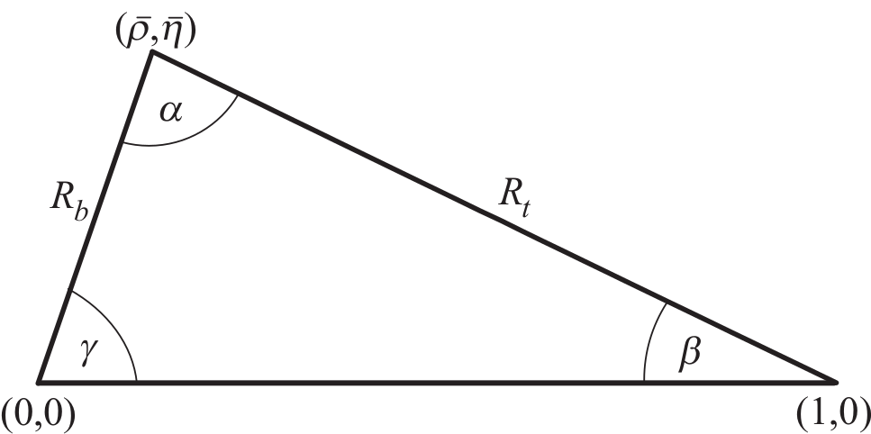
Figure 1: The Unitarity Triangle.

$R_{t}$ and $R_{b}$ can be solely expressed in terms of the angles $\beta$ and $\gamma$, as follows [29]

$$R_{t}=\frac{\sin\gamma}{\sin(\beta+\gamma)}\approx\sin\gamma,\qquad R_{b}=\frac{\sin\beta}{\sin(\beta+\gamma)}\approx\sin\beta\,.$$ (11)

We observe that $R_{t}$ depends dominantly on $\gamma$, while $R_{b}$ on $\beta$. These approximations follow from the experimental fact that $\beta+\gamma\approx 90^{\circ}$ and it is an excellent approximation to set $\sin(\beta+\gamma)=1$ in the formulae below although we will not do it in the numerical evaluations.

On the other hand:

$$\bar{\rho}=1-R_{t}\cos\beta,\qquad\bar{\eta}=R_{t}\sin\beta.$$ (12)

Consequently, $|V_{td}|$, $|V_{ub}|$ and $|V_{ts}|$ can be entirely expressed in terms of the parameters in (4)

$$\boxed{|V_{td}|=\lambda|V_{cb}|\sin\gamma,\qquad|V_{ub}|={\lambda\sqrt{\sigma}}|V_{cb}|\sin\beta,\qquad\sigma=\left(\frac{1}{1-\frac{\lambda^{2}}{2}}\right)^{2}\,,}$$ (13)

$$\boxed{|V_{ts}|=G(\beta,\gamma)|V_{cb}|,\qquad G(\beta,\gamma)=1+\frac{\lambda^{2}}{2}(1-2\sin\gamma\cos\beta)\,,}$$ (14)

where the approximations in (11) have been used and in the expression for $|V_{ts}|$ terms of ${\cal O}(\lambda^{4})$ have been neglected.

In turn, to an excellent accuracy of $0.2\%$ we also find for the imaginary part of $\lambda_{t}=V_{td}V^{*}_{ts}$

$$\boxed{{\rm{Im}}\lambda_{t}=|V_{ub}||V_{cb}|\sin\gamma={\lambda\sqrt{\sigma}}\sin\beta\sin\gamma|V_{cb}|^{2}\,.}$$ (15)

In order to increase the transparency of numerous formulae in our paper we will use the following reference values for the variables in (4)

$$\boxed{\lambda=0.225,\qquad|V_{cb}|=41.0\times 10^{-3},\qquad\beta=22.2^{\circ},\qquad\gamma=67^{\circ}\,.}$$ (16)

$m_{B_{s}}=5366.8(2)\text{MeV}$ [8]	$m_{B_{d}}=5279.58(17)\text{MeV}$ [8]
$\Delta M_{s}=17.749(20)\,\text{ps}^{-1}$ [8]	$\Delta M_{d}=0.5065(19)\,\text{ps}^{-1}$ [8]
$\Delta M_{K}=0.005292(9)\,\text{ps}^{-1}$ [8]	$m_{K^{0}}=497.61(1)\text{MeV}$ [8]
$S_{\psi K_{S}}=0.699(17)$ [8]	$F_{K}=155.7(3)\text{MeV}$ [46]
$|V_{us}|=0.2253(8)$ [8]	$|\epsilon_{K}|=2.228(11)\cdot 10^{-3}$ [8]
$F_{B_{s}}$ = $230.3(1.3)\text{MeV}$ [46]	$F_{B_{d}}$ = $190.0(1.3)\text{MeV}$ [46]
$B_{s}(4.18\,\text{GeV})=0.849(23)$ [47]	$B_{d}(4.18\,\text{GeV})=0.835(28)$ [47]
$\hat{B}_{s}=1.291(35)$ [33]	$\hat{B}_{d}=1.269(43)$ [33]
$m_{t}(m_{t})=162.83(67)\,\text{GeV}$ [7]	$m_{c}(m_{c})=1.279(13)\,\text{GeV}$
$S_{tt}(x_{t})=2.303$	$S_{ut}(x_{c},x_{t})=-1.983\times 10^{-3}$
$\eta_{tt}=0.55(2)$ [25]	$\eta_{ut}=0.402(5)$ [25]
$\kappa_{\varepsilon}=0.94(2)$ [48]	$\eta_{B}=0.55(1)$ [49, 50]
$\tau_{B_{s}}={1.515(4)}\,\text{ps}$ [8]	$\tau_{B_{d}}={1.519(4)}\,\text{ps}$ [8]

Table 1: Values of the experimental and theoretical quantities used as input parameters. For future updates see PDG [8] and HFLAV [46].

We collect other parameters used by us in Table 1.

2.2 Rare Kaon Decays

2.2.1 $K^{+}\rightarrow\pi^{+}\nu\bar{\nu}$ and $K_{L}\rightarrow\pi^{0}\nu\bar{\nu}$

For the branching ratios for $K^{+}\rightarrow\pi^{+}\nu\bar{\nu}$ and $K_{L}\rightarrow\pi^{0}\nu\bar{\nu}$ decays, the formulae with the exact dependence on the CKM parameters are given in [2]. However, for the search of the $|V_{cb}|$-independent relations it is useful to use the improved Wolfenstein parametrization and in particular the formulae in (12). Then the exact formulae for the branching ratios in questions are approximated by expressions that are particularly useful for our analysis and are shown in the following.

In the case of $K^{+}\rightarrow\pi^{+}\nu\bar{\nu}$ we recall the following formula [15, 51] that summarizes the dependence of $\mathcal{B}(K^{+}\rightarrow\pi^{+}\nu\bar{\nu})$ on $R_{t}$, $\beta$ and $V_{cb}$:

$$\mathcal{B}(K^{+}\rightarrow\pi^{+}\nu\bar{\nu})=\, (1+\Delta_{\text{EM}})\frac{\kappa_{+}}{\lambda^{8}}~{}|V_{cb}|^{4}X(x_{t})^{2}\Bigg{[}\sigma R^{2}_{t}\sin^{2}\beta$$

$$+\frac{1}{\sigma}\left(R_{t}\cos\beta+\frac{\lambda^{4}P_{c}(X)}{|V_{cb}|^{2}X(x_{t})}\right)^{2}\Bigg{]},$$ (17)

where [16, 17, 21, 22, 19]

$$\kappa_{+}={(5.173\pm 0.025)\times 10^{-11}\left[\frac{\lambda}{0.225}\right]^{8}},\qquad P_{c}(X)=(0.405\pm 0.024){\left[\frac{0.225}{\lambda}\right]^{4}}$$ (18)

and $\Delta_{\text{EM}}=-0.003$. The formula for $X(x_{t})$ is given in the Appendix A.

The expression in (2.2.1) can be considered as the fundamental formula for a correlation between $\mathcal{B}(K^{+}\rightarrow\pi^{+}\nu\bar{\nu})$, $\beta$ and any observable used to determine $R_{t}$ or equivalently $\gamma$ as seen in (11). It is valid also in all models with CMFV [52] where $X(x_{t})$ is replaced by a real function $X(x_{t},v)$ with $v$ collecting new physics parameters. When this formula was proposed twenty years ago, it contained significant uncertainties in $R_{t}$ determined through $\Delta M_{d}/\Delta M_{s}$, in $P_{c}(X)$ known only at NLO at that time, in $\kappa_{+}$ and in $|V_{cb}|$. The first three uncertainties have been significantly reduced since then leaving $|V_{cb}|$ as the main uncertainty. The above equation provides an approximation of the exact expression in [2] up to $1\%$.

In the case of $K_{L}\rightarrow\pi^{0}\nu\bar{\nu}$, using the exact expression for the branching ratio together with ${\rm Im}\lambda_{t}$ in (15), we have

$$\mathcal{B}(K_{L}\rightarrow\pi^{0}\nu\bar{\nu})=\kappa_{L}|V_{cb}|^{4}\left[\frac{{\lambda\sqrt{\sigma}}\sin\beta\sin\gamma}{\lambda^{5}}X(x_{t})\right]^{2},$$ (19)

where [22]

$$\kappa_{L}=(2.231\pm 0.013)\times 10^{-10}\left[\frac{\lambda}{0.225}\right]^{8}.$$ (20)

As we will see below, the fact that the function $X(x_{t})$ enters universally $K^{+}\rightarrow\pi^{+}\nu\bar{\nu}$ and $K_{L}\rightarrow\pi^{0}\nu\bar{\nu}$ branching ratios implies a practically $m_{t}$-independent relation between them.

Due to the absence of $P_{c}(X)$ in (19), $\mathcal{B}(K_{L}\to\pi^{0}\nu\bar{\nu})$ has essentially no theoretical uncertainties. It is only affected by parametric uncertainties coming from $|V_{cb}|$, $\beta$ and to a lesser extent from $\gamma$ and $m_{t}$.

For our purposes we follow [5] and cast the formulae (2.2.1) and (19) into a semi-numerical form that expresses the dominant parametric uncertainties. Relative to [5], in the case of $K^{+}\rightarrow\pi^{+}\nu\bar{\nu}$ we just change the central values of $|V_{cb}|$ and $\gamma$ into the reference ones in (16) and we evaluate the central value for the branching ratio using (2.2.1). Furthermore, we express the $\gamma$-dependence with a sine function. In the case of $K_{L}\rightarrow\pi^{0}\nu\bar{\nu}$, which was given in [5] in terms of $|V_{ub}|$, $|V_{cb}|$ and $\gamma$, we also trade the dependence on $|V_{ub}|$ for the one on $\beta$ using (13). We find

$${\mathcal{B}(K^{+}\rightarrow\pi^{+}\nu\bar{\nu})={(7.92\pm 0.28)}\times 10^{-11}\,\bigg{[}\frac{\left|V_{cb}\right|}{41.0\times 10^{-3}}\bigg{]}^{2.8}\bigg{[}\frac{\sin\gamma}{\sin 67^{\circ}}\bigg{]}^{1.39}},$$ (21)

$$\mathcal{B}(K_{L}\rightarrow\pi^{0}\nu\bar{\nu})={(2.61\pm 0.04)}\times 10^{-11}\, {\bigg{[}\frac{\left|V_{cb}\right|}{41.0\times 10^{-3}}\bigg{]}^{4}\bigg{[}\frac{\sin\gamma}{\sin(67^{\circ})}\bigg{]}^{2}\bigg{[}\frac{\sin\beta}{\sin({22.2^{\circ}})}\bigg{]}^{2}},$$ (22)

where we do not show explicitly the parametric dependence on $\lambda$ and set $\lambda=0.225$.

One can check using exact expressions that the $\lambda$ dependence of $\mathcal{B}(K^{+}\rightarrow\pi^{+}\nu\bar{\nu})$ is very weak, due to partial cancellations among different contributions. Even setting $\lambda=0$ this branching ratio changes only by 4%. The parametric relation for $\mathcal{B}(K_{L}\rightarrow\pi^{0}\nu\bar{\nu})$ is exact, while for $\mathcal{B}(K^{+}\rightarrow\pi^{+}\nu\bar{\nu})$ it gives an excellent approximation: with respect to (2.2.1), for the large ranges $38\leq|V_{cb}|\times 10^{3}\leq 43$ and $60^{\circ}\leq\gamma\leq 75^{\circ}$ it is accurate to $1.5\%$ scanning one parameter at a time and to $2.5\%$ letting both of them vary simultaneously in the corresponding intervals. The non-integer exponents, here and in similar equations in the following, are indeed fitted to describe as power-law functions of parameters some more complicated exact expressions, with the best possible accuracy. Note that (21) provides an even better approximation of the exact branching ratio [2], up to $1\%$ scanning one parameter at a time and to $1.5\%$ letting both of them vary simultaneously in the corresponding intervals. In the case of $\mathcal{B}(K^{+}\rightarrow\pi^{+}\nu\bar{\nu})$ the dependence on $\beta$ is very weak as one can verify even analytically by inspecting the formula (2.2.1). Therefore we have absorbed it into the non-parametric error.

The exact dependence of both branching ratios on $|V_{cb}|$ for different $\gamma$ and $\beta$ is shown in Fig. 2. We observe the pattern summarized at the beginning of our paper. Furthermore, one can notice that the branching ratio for $K^{+}\rightarrow\pi^{+}\nu\bar{\nu}$ is almost exactly independent of the $\beta$ angle, as commented above. One can also see that the largest uncertainties on these branching ratios are due to the $|V_{cb}|$ parameter: the elimination of this source of error is the main focus of our work.

The dependence of the branching ratios for $K^{+}\rightarrow\pi^{+}\nu\bar{\nu}$ and $K_{L}\rightarrow\pi^{0}\nu\bar{\nu}$ on $\gamma$, $\beta$ and $|V_{cb}|$ has also been studied in [28]. There are other useful results in that paper, in [5], [37] and [53]. In the latter paper several simplified models have been presented.

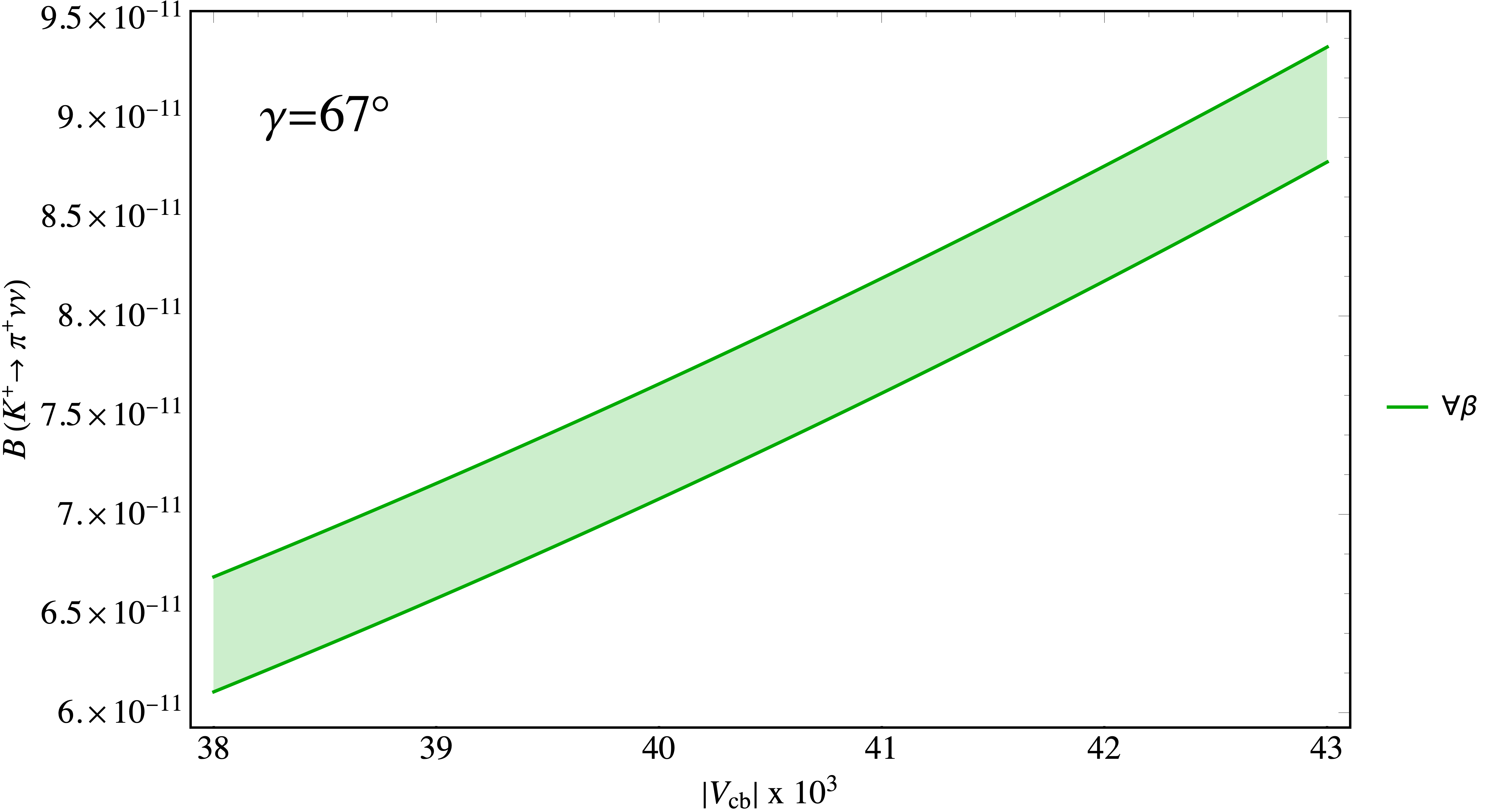
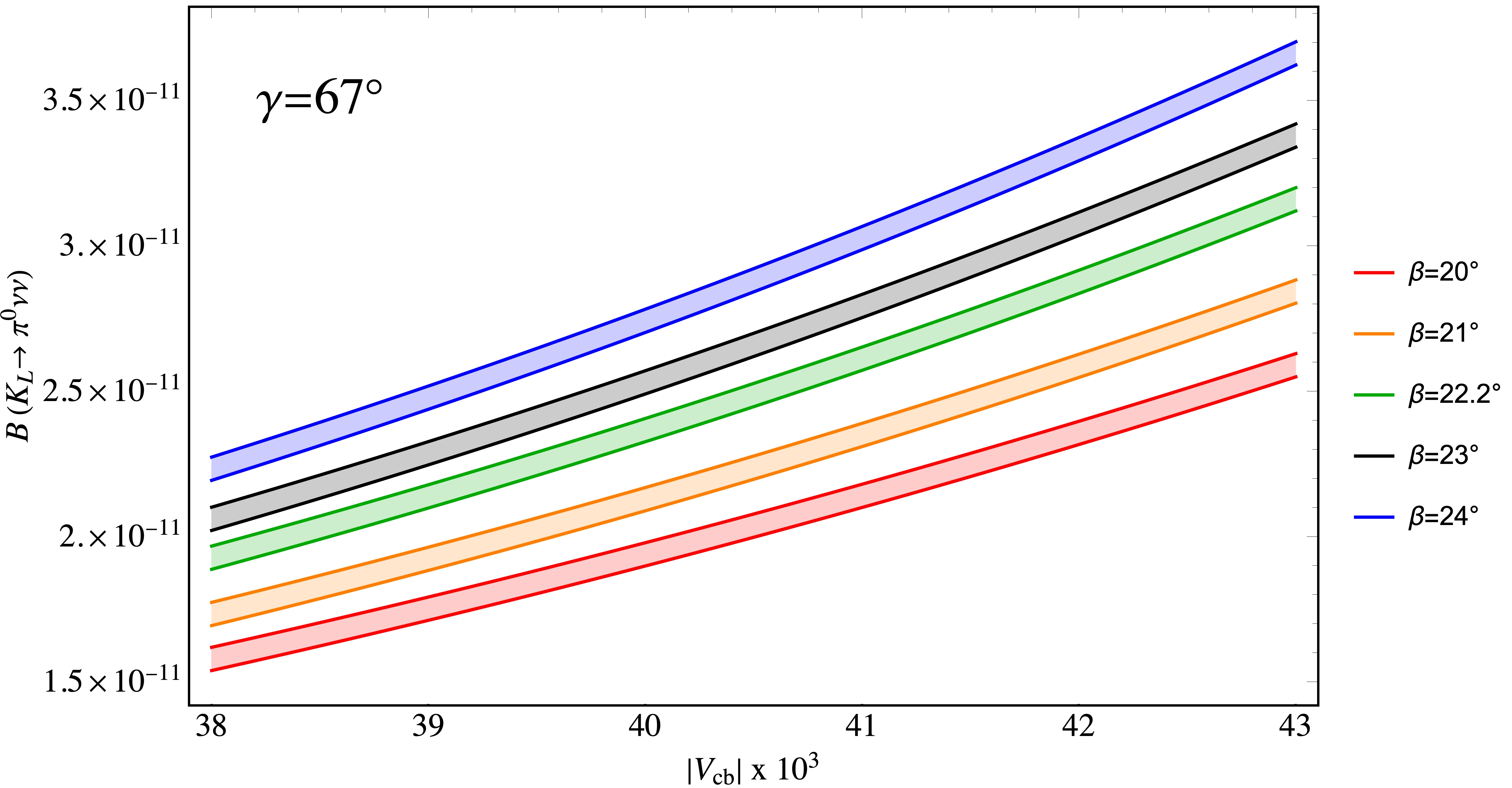
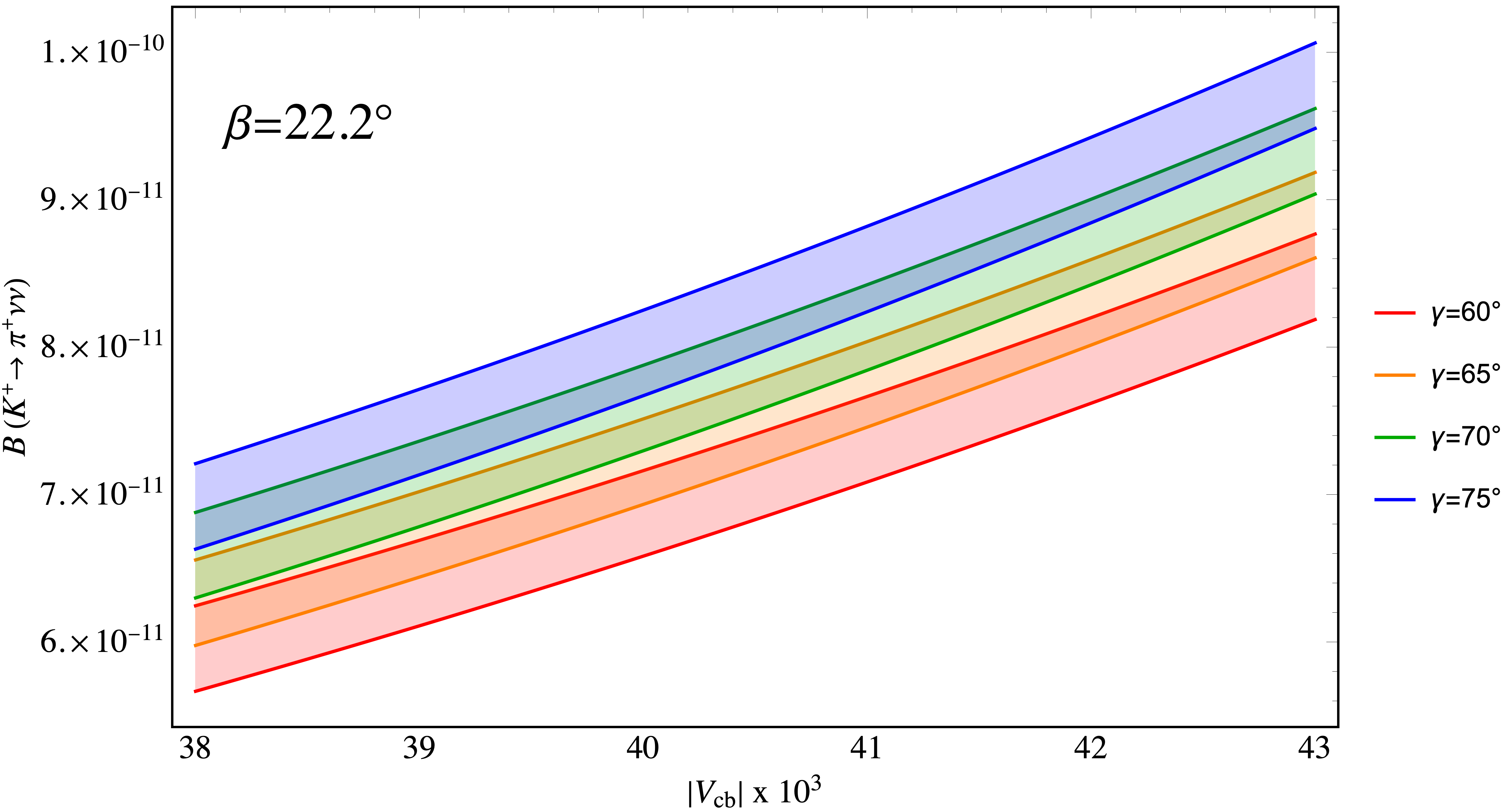
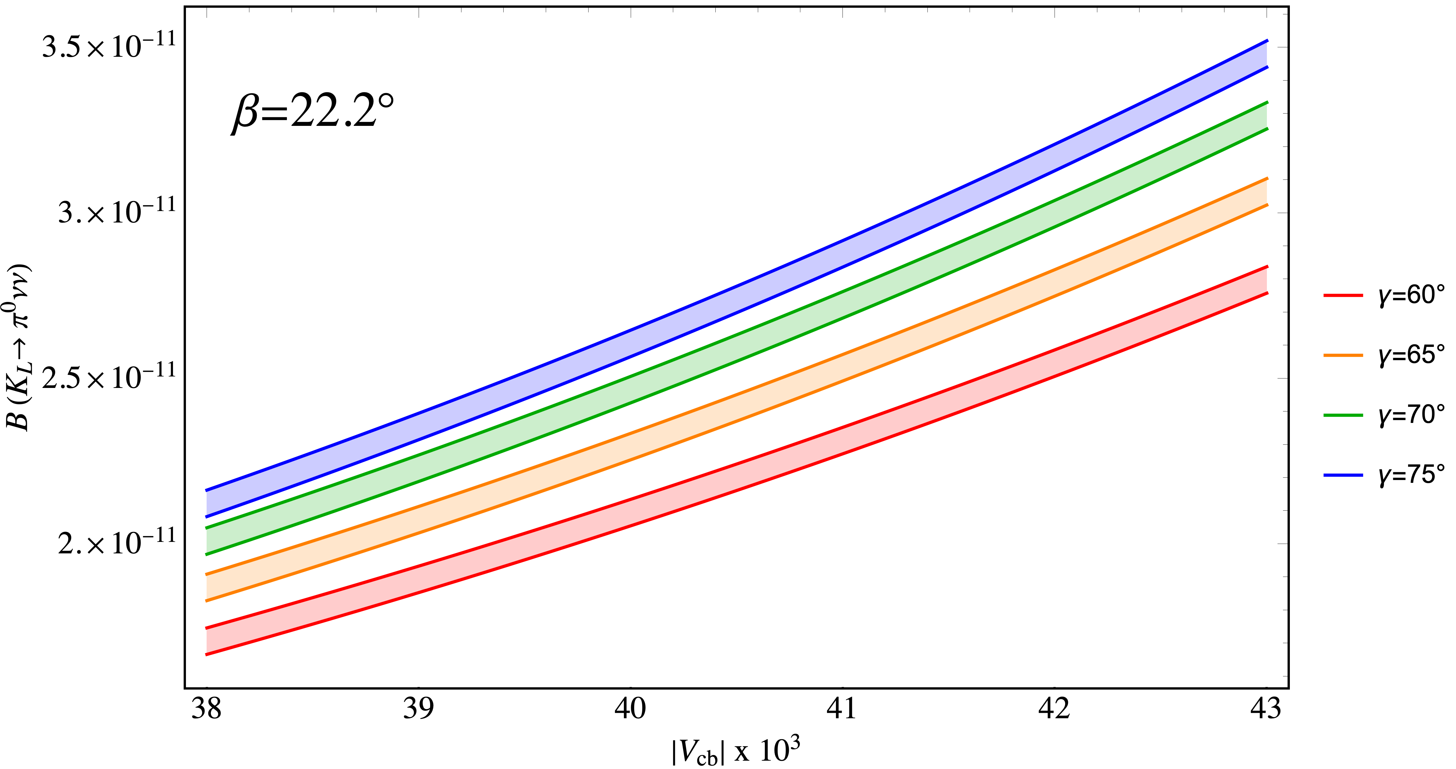
Figure 2: The dependence of the branching ratios $\mathcal{B}(K^{+}\rightarrow\pi^{+}\nu\bar{\nu})$ (left panels) and $\mathcal{B}(K_{L}\rightarrow\pi^{0}\nu\bar{\nu})$ (right panels) on $|V_{cb}|$ for different values of $\beta=20.0^{\circ},21.0^{\circ},22.0^{\circ},23.0^{\circ},24.0^{\circ}$ at fixed $\gamma=67^{\circ}$ and for different values of $\gamma=60.0^{\circ},65.0^{\circ},70.0^{\circ},75^{\circ}$ at fixed $\beta=22.2^{\circ}$ . The width of the bands represents the uncertainties whose origin is not related to the $\gamma$, $\beta$ and $|V_{cb}|$ parameters.

The theoretically clean character of $K_{L}\rightarrow\pi^{0}\nu\bar{\nu}$ and its very strong dependence on $|V_{cb}|$ could in principle allow a precise measurement of $|V_{cb}|$ [35] by inverting (19) to obtain

$$|V_{cb}|^{2}=\sqrt{\frac{\mathcal{B}(K_{L}\rightarrow\pi^{0}\nu\bar{\nu})}{\kappa_{L}}}\frac{\lambda^{5}}{{\lambda\sqrt{\sigma}}\sin\beta\sin\gamma X(x_{t})}.$$ (23)

Note that a $10\%$ measurement of the branching ratio allows to determine $|V_{cb}|$ with the precision of $2.5\%$. This strategy cannot be executed at present and it is likely polluted by NP contributions. But inserting (23) into (2.2.1) allows to derive the expression for $K^{+}\rightarrow\pi^{+}\nu\bar{\nu}$ branching ratio in terms of the $K_{L}\rightarrow\pi^{0}\nu\bar{\nu}$ one.

To this end it is useful to define the “reduced” branching ratios [34]

$$B_{1}=\frac{\mathcal{B}(K^{+}\rightarrow\pi^{+}\nu\bar{\nu})}{\kappa_{+}(1+\Delta_{\text{EM}})},\qquad B_{2}=\frac{\mathcal{B}(K_{L}\rightarrow\pi^{0}\nu\bar{\nu})}{\kappa_{L}}.$$ (24)

We find then

$$B_{1}=B_{2}\left[1+\frac{1}{\sigma^{2}}(\cot\beta+\frac{\sqrt{\sigma}P_{c}(X)}{\sqrt{B_{2}}})^{2}\right],$$ (25)

with $\sigma$ defined in (13).

It should be emphasized that this relation is independent of $|V_{cb}|$, $\gamma$ and $m_{t}$. However, as (2.2.1) is not exact also this relation is an approximation. Albeit, an excellent one, with only $1\%$ error. Therefore it can be used in principle to determine the angle $\beta$, the sole parameter in this formula [34]. Here we just present it as an elegant formula for the well known relation between $K^{+}\rightarrow\pi^{+}\nu\bar{\nu}$ branching ratio and the $K_{L}\rightarrow\pi^{0}\nu\bar{\nu}$ one within the SM and models with CMFV, stressing its very weak dependence on $|V_{cb}|$, $\gamma$ and $m_{t}$.

Alternatively using (21) and (22) one can eliminate $|V_{cb}|$ to find

$$\mathcal{B}(K^{+}\rightarrow\pi^{+}\nu\bar{\nu}) ={(7.92\pm 0.30)}\times 10^{-11}\left[\frac{\sin 22.2^{\circ}}{\sin\beta}\right]^{1.4}\left[\frac{\mathcal{B}(K_{L}\rightarrow\pi^{0}\nu\bar{\nu})}{{2.61}\times 10^{-11}}\right]^{0.7}.$$ (26)

This formula is also independent of $\gamma$ and reproduces (25) with an accuracy in the ballpark of 4%; it is provided here in order to show the correlation between the two observables in a more transparent manner, while for the numerical analysis their exact expressions are used. The uncertainty shown here has been computed by propagating the non-parametric errors of the two involved branching ratios. The same procedure will be used for all the equations presenting correlations or ratios between observables. The above relation motivates us to define the approximately $|V_{cb}|$-independent ratio

$$\boxed{R_{0}=\frac{\mathcal{B}(K^{+}\rightarrow\pi^{+}\nu\bar{\nu})}{\mathcal{B}(K_{L}\rightarrow\pi^{0}\nu\bar{\nu})^{0.7}}\,,}$$ (27)

whose $\beta$ dependence is shown in Fig. 3. The coloured bands represent the variation of $R_{0}$, with fixed $\gamma$, when $|V_{cb}|$ takes values in $38<|V_{cb}|\times 10^{3}<43$, which is smaller than 0.5%. Different bands correspond to various $\gamma$ values: when $60^{\circ}<\gamma<75^{\circ}$ the variation of $R_{0}$ is within the per-cent level. The numerical analysis, thus, shows that $R_{0}$ is indeed $|V_{cb}|$ and $\gamma$ independent to an excellent accuracy. On the other hand, the uncertainty related to the errors on parameters different from $\beta$, $\gamma$ and $|V_{cb}|$, represented in gray in the figure, is much larger, in the ballpark of 5%. Restricting the value of $\beta$ to the one in (5) and including all other uncertainties we find

$$(R_{0})_{\rm SM}={(2.03\pm 0.11)}\times 10^{-3}\,.$$ (28)

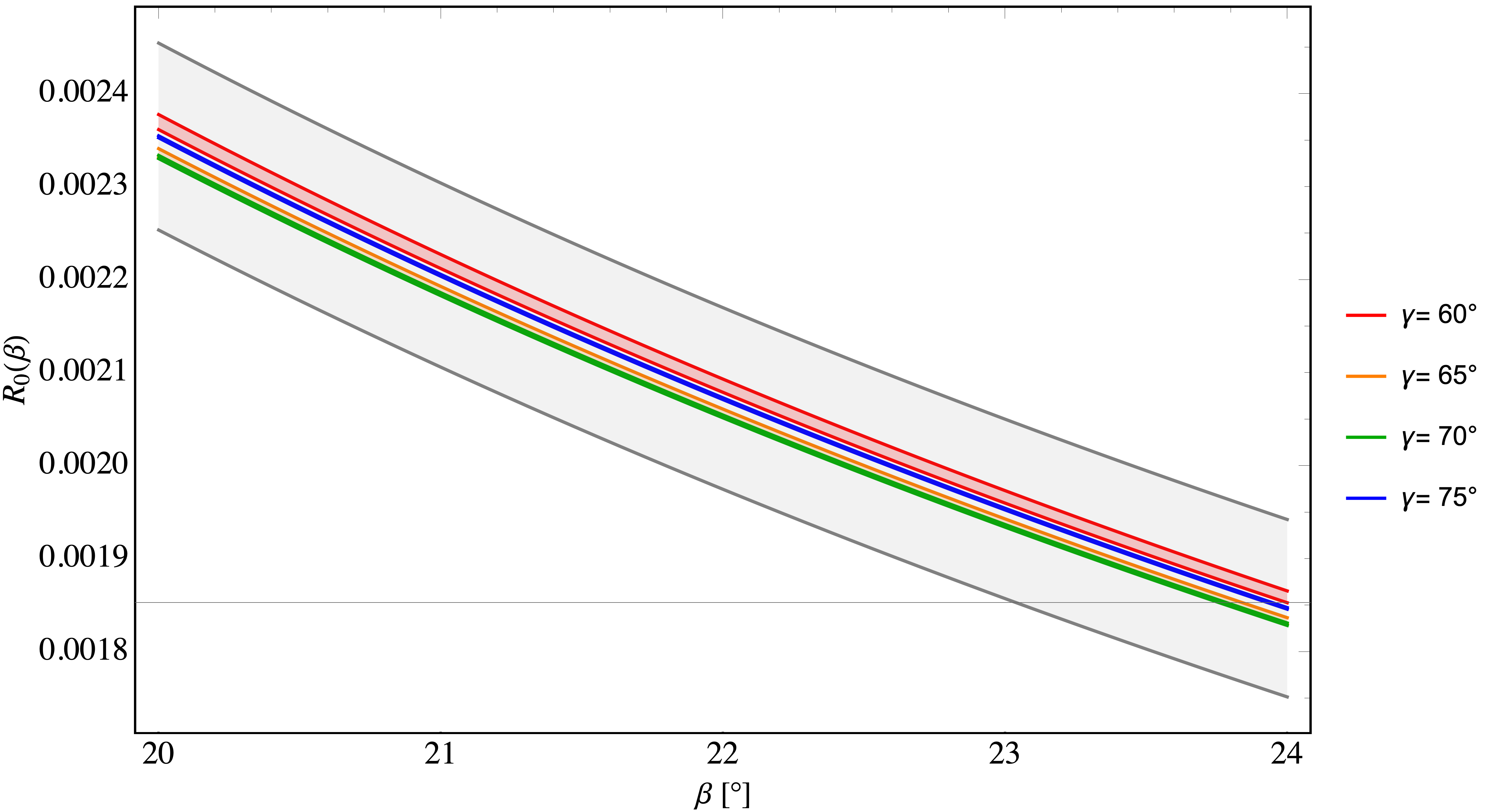
Figure 3: The ratio $R_{0}$ given in (27) as a function of $\beta$ for different values of $\gamma$ within the SM. The coloured bands correspond to $38\leq|V_{cb}|\times 10^{3}\leq 43$. The gray band represents the non-parametric uncertainty.

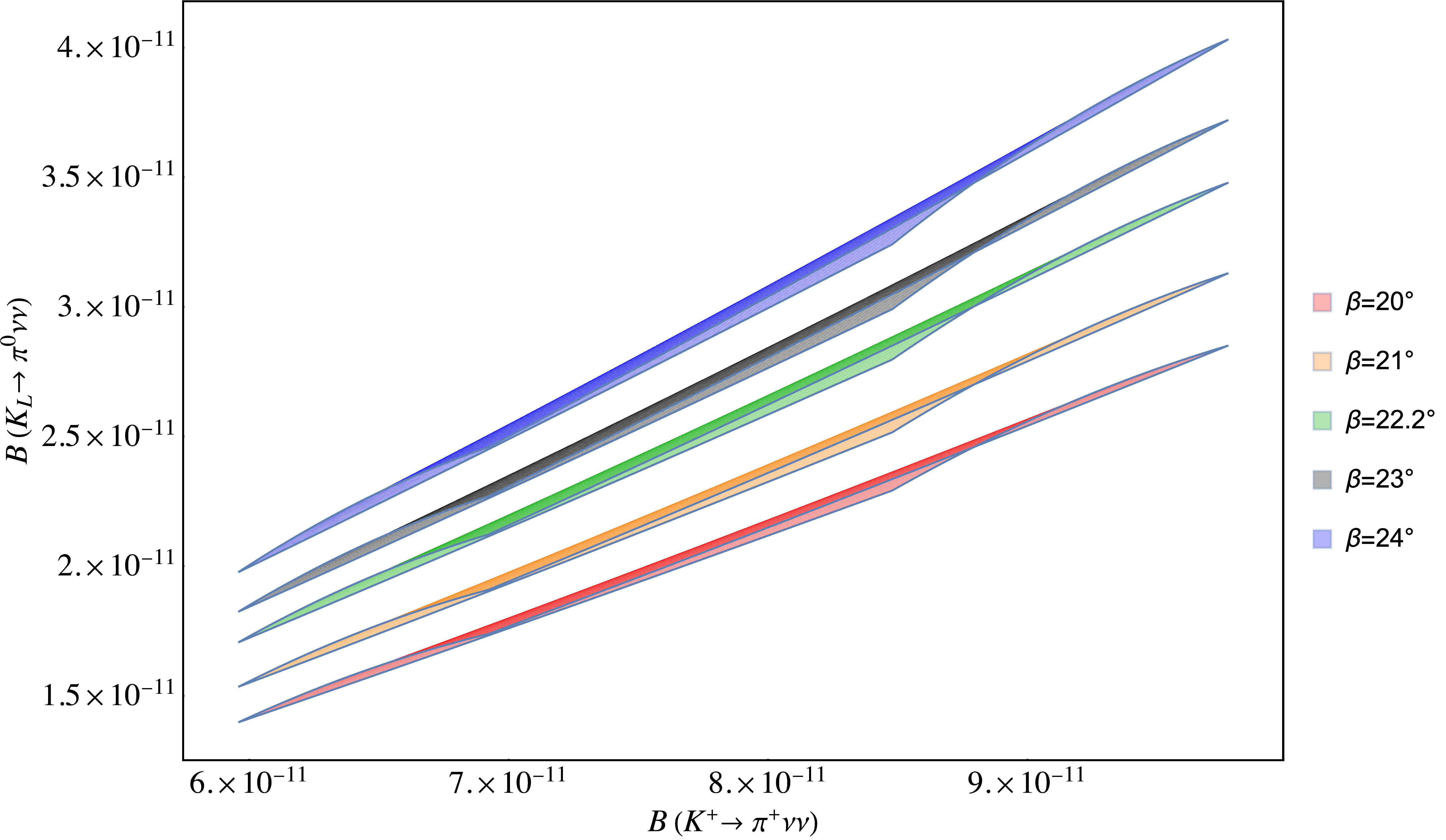
Figure 4: The correlation between branching ratios for $K_{L}\rightarrow\pi^{0}\nu\bar{\nu}$ and $K^{+}\rightarrow\pi^{+}\nu\bar{\nu}$ as given in (25) for different values of $\beta$ within the SM. The ranges of branching ratios correspond to $38\leq|V_{cb}|\times 10^{3}\leq 43$ and $60^{\circ}\leq\gamma\leq 75^{\circ}$.

In Fig. 4 we show the usual plot, representing (25), that correlates the branching ratios for $K_{L}\rightarrow\pi^{0}\nu\bar{\nu}$ and $K^{+}\rightarrow\pi^{+}\nu\bar{\nu}$ in the SM for fixed values of $\beta$ [34]. The SM values depend on $|V_{cb}|$ but the positions of the straight lines depend basically only on $\beta$. Moreover, they have practically a universal slope. Also the dependence on $\gamma$ almost perfectly cancels out. However, the cancellation is exact using (2.2.1) for $\mathcal{B}(K^{+}\rightarrow\pi^{+}\nu\bar{\nu})$, while one can see in the plot that using the exact expression there is a residual weak $\gamma$-dependence. The uncertainties not related to $|V_{cb}|$, $\gamma$ and $\beta$ are not shown in this figure.

A given line in Fig. 4 reminds us at first sight the correlation between $K^{+}\rightarrow\pi^{+}\nu\bar{\nu}$ and $K_{L}\rightarrow\pi^{0}\nu\bar{\nu}$ branching ratios in models with MFV [54] for $X(x_{t})>0$ and in the plots showing this correlations in different models, like in [53, 55], the SM value is represented by a point. But one should realize that in that papers the lines are obtained by varying $X$ while keeping $|V_{cb}|$ and $\beta$ fixed. On the other hand in Fig. 4 while $X$ is kept at its SM value both $|V_{cb}|$ and $\beta$ are varied. In other words the SM point in the plots in [53, 55] and similar plots found in the literature is rather uncertain and Fig. 4 signals this uncertainty. Inspecting formulae (2.2.1) and (19) one finds that for fixed $\beta$ the position on a given straight line Fig. 4 is determined by the combination $|V_{cb}|^{2}X(x_{t})$.

2.2.2 $K_{S}\to\mu^{+}\mu^{-}$

This decay provides another sensitive probe of imaginary parts of short-distance couplings. Its branching ratio receives long-distance (LD) and short-distance (SD) contributions, which are added incoherently in the total rate [56, 57]. This is in contrast to the decay $K_{L}\to\mu^{+}\mu^{-}$, where LD and SD amplitudes interfere with each other; moreover ${\cal B}(K_{L}\to\mu^{+}\mu^{-})$ is sensitive to real parts of couplings. The SD part of ${\cal B}(K_{S}\to\mu^{+}\mu^{-})$ is given as $(\lambda_{t}=V^{*}_{ts}V_{td})$

$${\cal B}(K_{S}\to\mu^{+}\mu^{-})_{\rm SD}=\tau_{K_{S}}\frac{G_{F}^{2}\alpha^{2}}{8\pi^{3}\sin^{4}\theta_{W}}m_{K}F_{K}^{2}\sqrt{1-4\frac{m^{2}_{\mu}}{m_{K}^{2}}}m_{\mu}^{2}\,\mbox{Im}^{2}\left[\lambda_{t}Y(x_{t})\right],$$ (29)

which, applying (15), can be expressed as

$${\cal B}(K_{S}\to\mu^{+}\mu^{-})_{\rm SD}=1.04\times 10^{-5}|V_{cb}|^{4}\left[{\lambda\sqrt{\sigma}}\,{\sin\gamma\sin\beta}\,Y(x_{t})\right]^{2}\,,$$ (30)

where $Y(x_{t})$ is given in the Appendix A.

In 2019 the LHCb collaboration improved the upper bound on $K_{S}\to\mu^{+}\mu^{-}$ by one order of magnitude [58]

$${\cal B}(K_{S}\to\mu^{+}\mu^{-})_{\rm LHCb} <0.8\,(1.0)\times 10^{-9} \mbox{at}\;90\%\,(95\%)\;\mbox{C.L.}$$ (31)

to be compared with the SM prediction [57, 59]

$${\cal B}(K_{S}\to\mu^{+}\mu^{-})_{\rm SM} =(4.99_{\rm LD}+0.19_{\rm SD})\times 10^{-12}=(5.2\pm 1.5)\times 10^{-12}.$$ (32)

Recently it has been demonstrated in [24] that the short distance contribution in (29) can be extracted from data offering us still another precision observable. Here we point out that in the SM the ratio (see (19) and (30))

$$\boxed{R_{\rm SL}=\frac{{\cal B}(K_{S}\to\mu^{+}\mu^{-})_{\rm SD}}{{\cal B}(K_{L}\rightarrow\pi^{0}\nu\bar{\nu})}=1.55\times 10^{-2}\,\left[\frac{\lambda}{0.225}\right]^{2}\left[\frac{Y(x_{t})}{X(x_{t})}\right]^{2}\,}$$ (33)

is independent of any SM parameter except for $m_{t}$ and $\lambda$ which are both precisely known.

2.3 Correlations with $B_{s,d}\to\mu^{+}\mu^{-}$

Using the exact formulae in [2] that are based on the calculations over three decades by several groups [12, 15, 40, 41, 60, 61, 42, 62] the dependence of the branching ratio for $B_{s}\to\mu^{+}\mu^{-}$ on the input parameters involved can be transparently summarized as follows [41]

$$\overline{\mathcal{B}}(B_{s}\to\mu^{+}\mu^{-})_{\rm SM}=({3.47}\pm 0.06)\times 10^{-9}\left(\frac{F_{B_{s}}}{{230.3}\text{MeV}}\right)^{2}\left|\frac{V_{tb}^{*}V_{ts}}{{0.0402}}\right|^{2}\bar{R}_{s}$$ (34)

where

$$\bar{R}_{s}=\left(\frac{\tau_{B_{s}}}{{1.515}{\rm ps}}\right)\left(\frac{{0.935}}{r(y_{s})}\right)\left(\frac{m_{t}(m_{t})}{162.83\,\text{GeV}}\right)^{3.02}\left(\frac{\alpha_{s}(M_{Z})}{0.1184}\right)^{0.032}\,.$$ (35)

Here $r(y_{s})$ summarizes $\Delta\Gamma_{s}$ effects with $r(y_{s})={0.935}\pm 0.007$ within the SM [63, 64, 65].

Similarly one finds [41]

$${\mathcal{B}}(B_{d}\to\mu^{+}\mu^{-})_{\rm SM}=({0.968}\pm 0.02)\times 10^{-10}\left(\frac{F_{B_{d}}}{{190.0}\text{MeV}}\right)^{2}\left|\frac{V_{tb}^{*}V_{td}}{0.00848}\right|^{2}\bar{R}_{d}\,.$$ (36)

As to an excellent accuracy $r(y_{d})=1$, one has this time

$$\bar{R}_{d}=\left(\frac{\tau_{B_{d}}}{1.519{\rm ps}}\right)\left(\frac{m_{t}(m_{t})}{162.83\,\text{GeV}}\right)^{3.02}\left(\frac{\alpha_{s}(M_{Z})}{0.1184}\right)^{0.032}\,.$$ (37)

These two branching ratios are shown as functions of $|V_{cb}|$ in Fig. 5, for different values of $\gamma$ with fixed $\beta$ and viceversa. One can notice that the $\beta$ dependence is almost negligible for both observables, while the $\gamma$ dependence is stronger, especially in the case of the $B_{d}$ decay. Furthermore, very importantly, it is evident that the size of possible anomaly in $B_{s}\to\mu^{+}\mu^{-}$ depends strongly on the value of $|V_{cb}|$ as emphasized recently in [33]. For the values of $|V_{cb}|$ from inclusive determinations an anomaly at the level of $2\sigma$ can be concluded [66, 67], while for $|V_{cb}|$ values smaller than $40.3\times 10^{-3}$ the SM prediction agrees with the experimental measurement of $B_{s}\to\mu^{+}\mu^{-}$ decay at $1\sigma$ level. Finally, for the FLAG’s $|V_{cb}|$ value in the ballpark of $39\times 10^{-3}$ perfect agreement of the SM with the data is obtained. Only by constructing the ratio $R_{s}$ in (95) an anomaly at the level of $2.2\sigma$ independently of $|V_{cb}|$ can be concluded [33]. See also comments after (8).

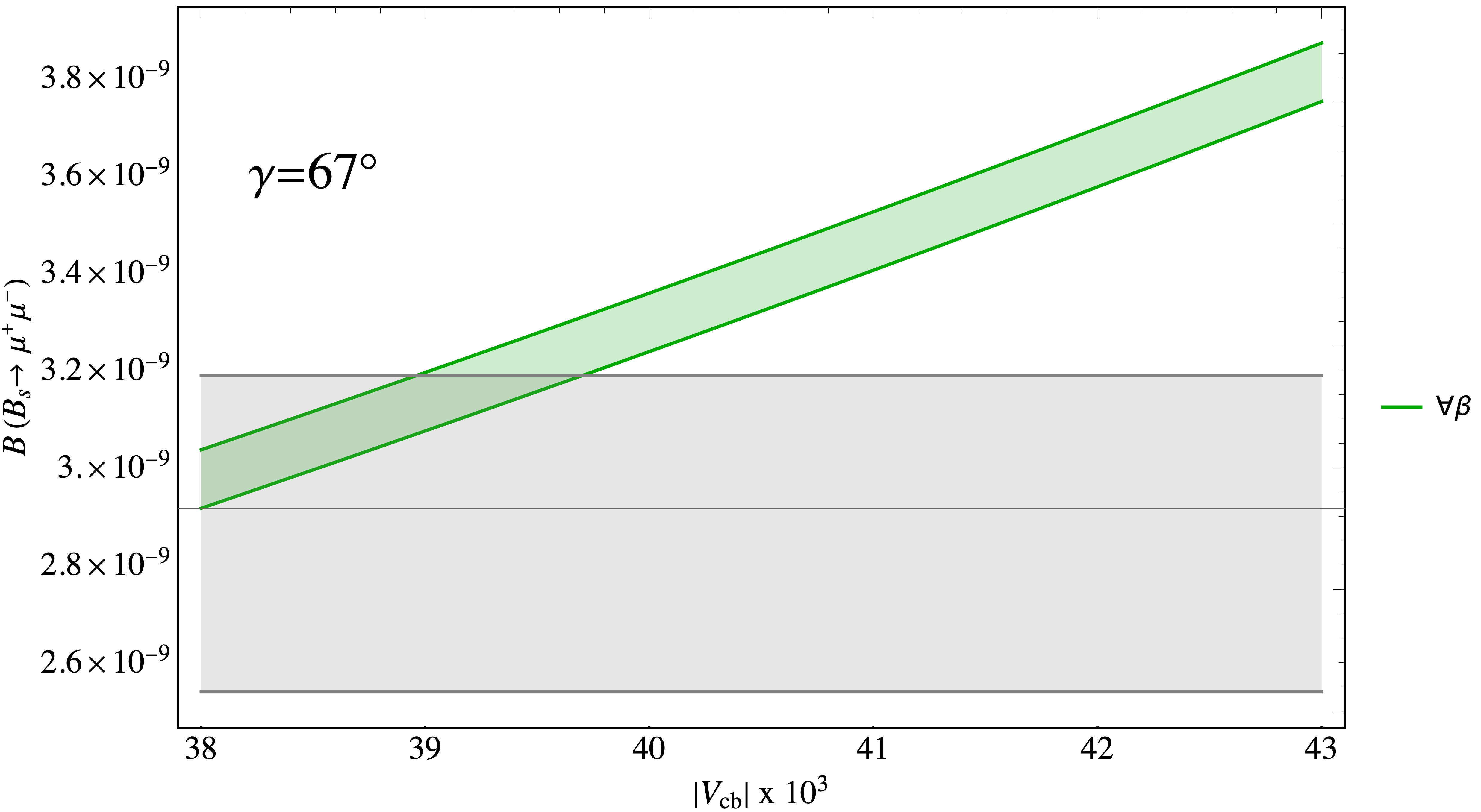
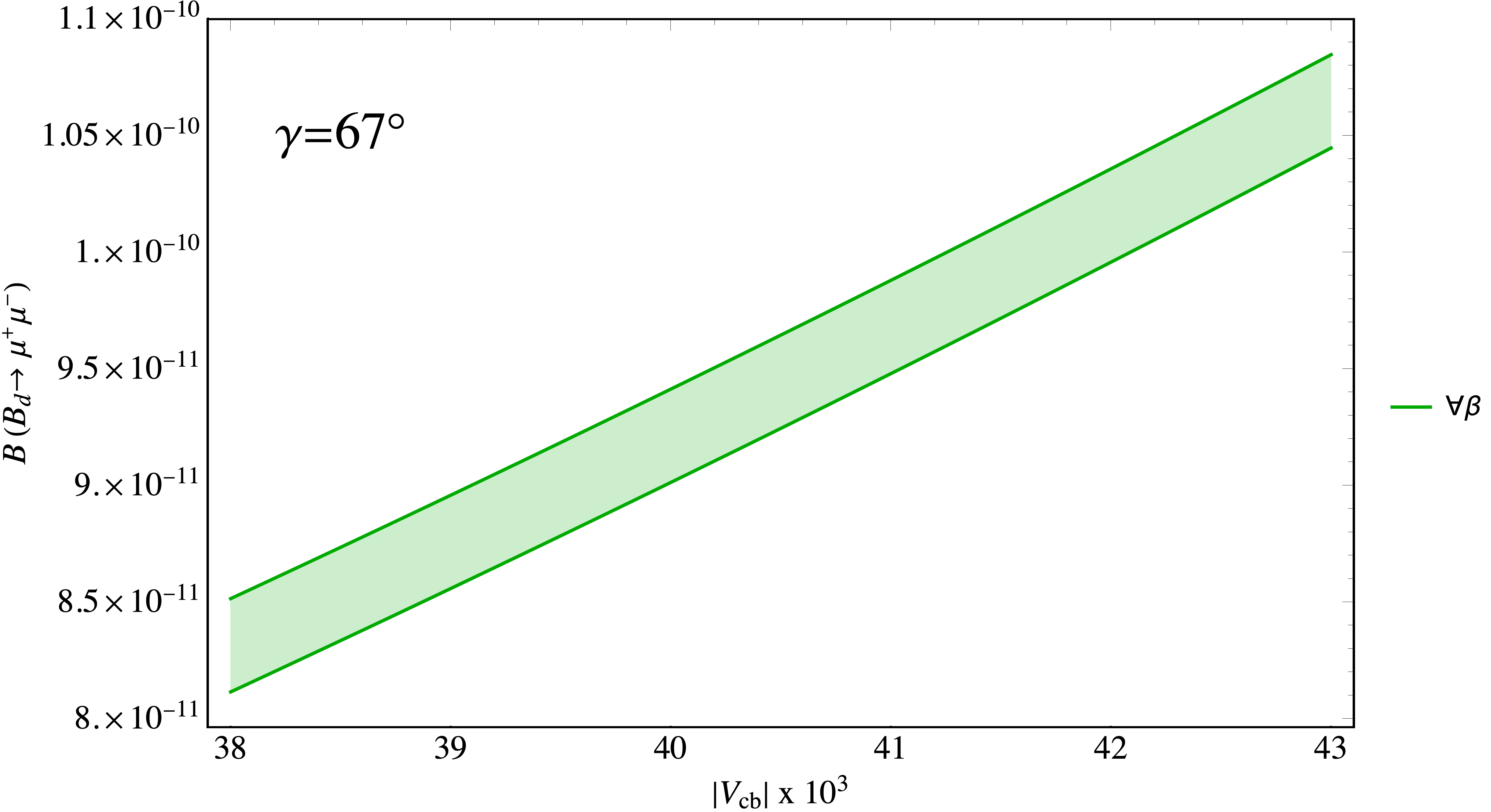
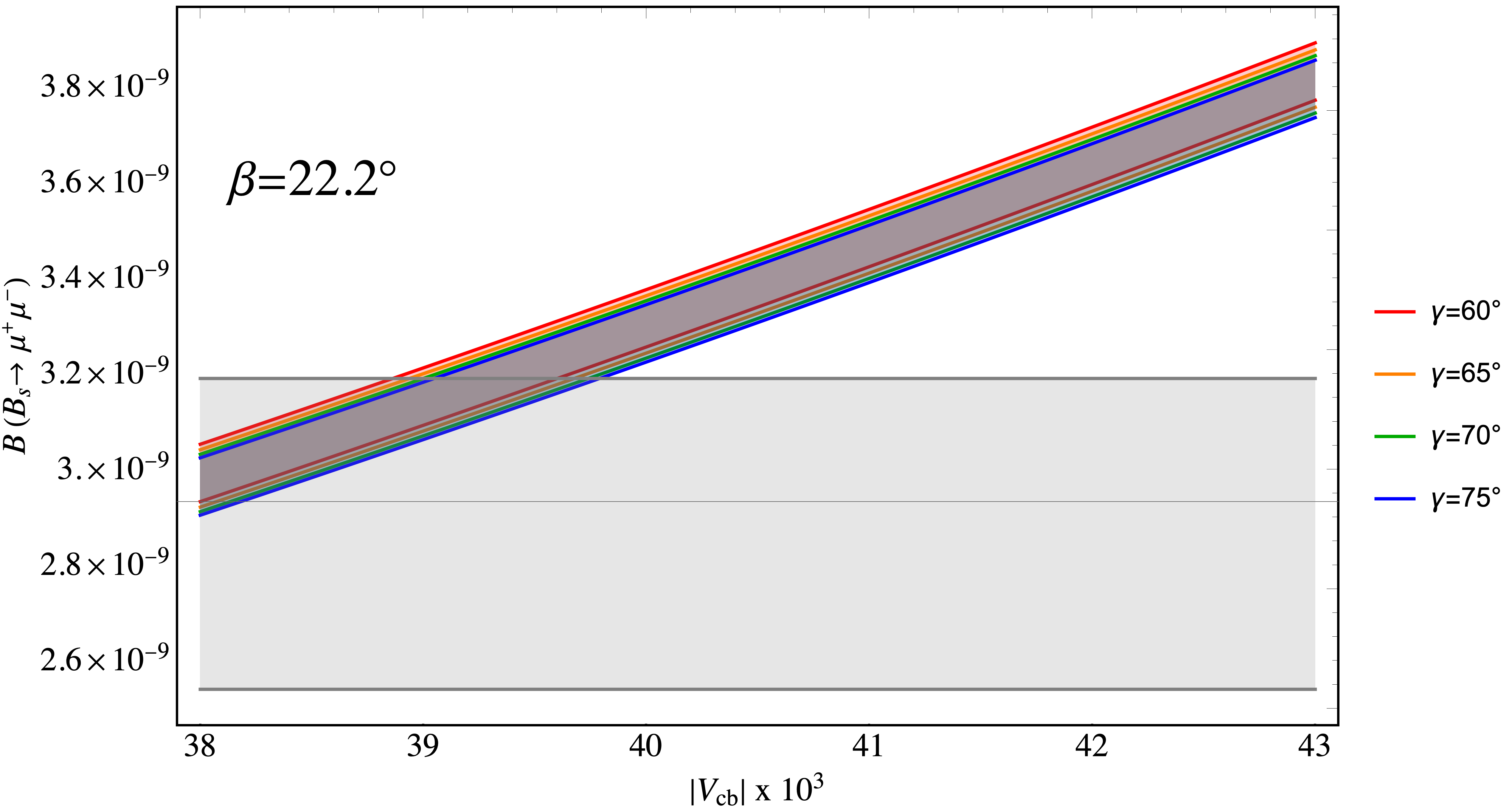
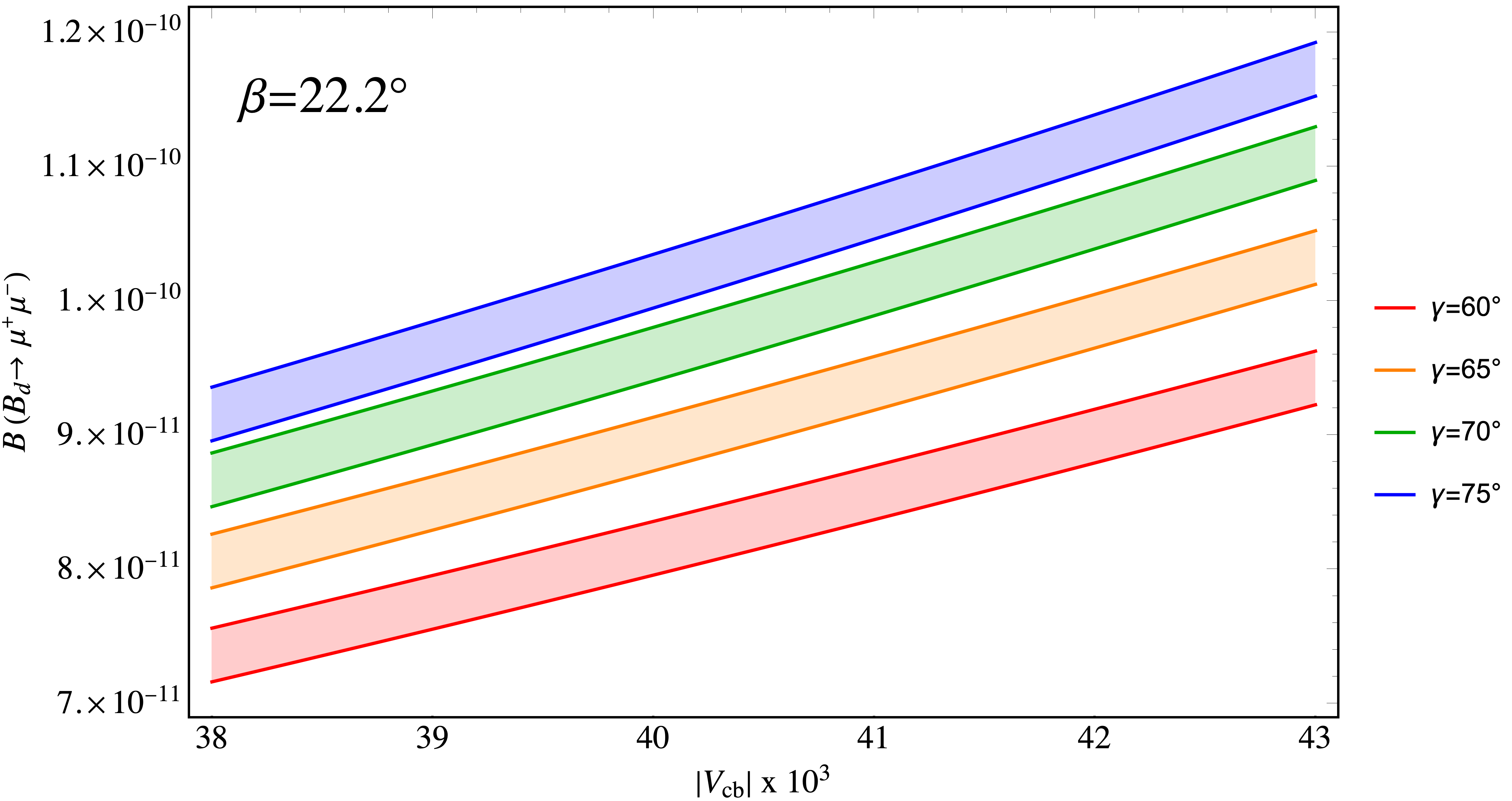
Figure 5: The dependence of the branching ratios $\overline{\mathcal{B}}(B_{s}\to\mu^{+}\mu^{-})$ (left panels) and ${\mathcal{B}}(B_{d}\to\mu^{+}\mu^{-})$ (right panels) on $|V_{cb}|$ for different values of $\beta=20.0^{\circ},21.0^{\circ},22.0^{\circ},23.0^{\circ},24.0^{\circ}$ at fixed $\gamma=67^{\circ}$ and for different values of $\gamma=60.0^{\circ},65.0^{\circ},70.0^{\circ},75^{\circ}$ at fixed $\beta=22.2^{\circ}$ . The width of the bands represents the uncertainties whose origin is not related to the $\gamma$, $\beta$ and $|V_{cb}|$ parameters. The gray horizontal bands in the left panels shows the $1\sigma$ experimental range (see (46)).

Following the same strategy as for the analysis of the $\mathcal{B}(K^{+}\rightarrow\pi^{+}\nu\bar{\nu})$-$\mathcal{B}(K_{L}\rightarrow\pi^{0}\nu\bar{\nu})$ correlation, one can take advantage from the fact that $\overline{\mathcal{B}}(B_{s}\to\mu^{+}\mu^{-})$ is an exact quadratic function of $|V_{cb}|$ (see (14) and (34)), and find

$$|V_{cb}|^{2}=\frac{\overline{\mathcal{B}}(B_{s}\to\mu^{+}\mu^{-})}{{2.14}\times 10^{-6}\bar{R}_{s}}\left(\frac{{230.3}\text{MeV}}{F_{B_{s}}}\frac{1}{G(\beta,\gamma)}\right)^{2}\,,$$ (38)

where $G(\beta,\gamma)$ is defined as in (14).

Inserting the above expression into (2.2.1), one can derive the relation between the branching ratios for $K^{+}\to\pi^{+}\nu\bar{\nu}$ and $B_{s}\to\mu^{+}\mu^{-}$ decays. Defining

$$B_{3}=\frac{\overline{\mathcal{B}}(B_{s}\to\mu^{+}\mu^{-})}{{2.14}\times 10^{-6}{\bar{R}_{s}}}\,,$$ (39)

one obtains

$$B_{1}=\frac{X(x_{t})^{2}}{\lambda^{8}}B_{3}^{2}\left(\frac{{230.3}\text{MeV}}{F_{B_{s}}}\frac{1}{G(\beta,\gamma)}\right)^{4}$$

$$\times\Big{[} \sigma\sin^{2}\gamma\sin^{2}\beta+\frac{1}{\sigma}\left(\sin\gamma\cos\beta+\frac{\lambda^{4}P_{c}(X)}{B_{3}X(x_{t})}\left(\frac{F_{B_{s}}}{{230.3}\text{MeV}}G(\beta,\gamma)\right)^{2}\right)^{2}\Big{]}\,,$$ (40)

with $\sigma$ and $G(\beta,\gamma)$ defined previously.

Alternatively using (21) and (34) one can eliminate $|V_{cb}|$ to find [5]

$$\mathcal{B}(K^{+}\rightarrow\pi^{+}\nu\bar{\nu}) ={(7.92\pm 0.34)}\times 10^{-11}\left[\frac{\sin\gamma}{\sin 67^{\circ}}\right]^{1.39}\left[\frac{G(22.2^{\circ},67^{\circ})}{G(\beta,\gamma)}\right]^{2.8}$$

$$\qquad\qquad\qquad\quad\times\left[\frac{\overline{\mathcal{B}}(B_{s}\to\mu^{+}\mu^{-})}{{3.47}\times 10^{-9}\bar{R}_{s}}\right]^{1.4}\left[\frac{{230.3}\text{MeV}}{F_{B_{s}}}\right]^{2.8}.$$ (41)

The above expression reproduces the correlation of (2.3) with an accuracy of less than $0.5\%$, when $\gamma$ varies in the range $60^{\circ}\leq\gamma\leq 75^{\circ}$ and the branching ratio $\overline{\mathcal{B}}(B_{s}\to\mu^{+}\mu^{-})$ takes values in its $1\sigma$ interval. Here, the dependence on $\gamma$ is slightly different with respect to (21), due to the $\gamma$ dependence of the $|V_{ts}|$ element entering in $\overline{\mathcal{B}}(B_{s}\to\mu^{+}\mu^{-})$.

Proceeding in the same manner with $B_{d}\to\mu^{+}\mu^{-}$ and defining

$$B_{4}=\frac{\mathcal{B}(B_{d}\to\mu^{+}\mu^{-})}{{1.34}\times 10^{-6}\bar{R}_{d}}\,,$$ (42)

we find analogous equations to (2.3) and (41), namely

$$B_{1}=\frac{X(x_{t})^{2}}{\lambda^{8}}B_{4}^{2}\left(\frac{{190.0}\text{MeV}}{F_{B_{d}}}\frac{1}{\lambda}\right)^{4}\frac{1}{\sin^{2}\gamma}$$

$$\times\Big{[} \sigma\sin^{2}\beta+\frac{1}{\sigma}\left(\cos\beta+\frac{\lambda^{4}P_{c}(X)}{B_{4}X(x_{t})}\left(\frac{F_{B_{d}}}{{190.0}\text{MeV}}\lambda\right)^{2}\sin\gamma\right)^{2}\Big{]}\,$$ (43)

and

$$\mathcal{B}(K^{+}\rightarrow\pi^{+}\nu\bar{\nu}) ={(7.92\pm 0.36)}\times 10^{-11}\left[\frac{\sin(67^{\circ})}{\sin\gamma}\right]^{1.41}$$

$$\qquad\qquad\qquad\quad\times\left[\frac{{\mathcal{B}}(B_{d}\to\mu^{+}\mu^{-})}{{0.968}\times 10^{-10}\bar{R}_{d}}\right]^{1.4}\left[\frac{{190.0}\text{MeV}}{F_{B_{d}}}\right]^{2.8}.$$ (44)

The last expression provides an approximation of (2.3) accurate to $0.5\%$, when $\gamma$ varies in the range $60^{\circ}\leq\gamma\leq 75^{\circ}$ and the branching ratio ${\mathcal{B}}(B_{d}\to\mu^{+}\mu^{-})$ takes values in its $1\sigma$ interval.

Note that the simple relations in (41) and (44) are independent of $|V_{cb}|$ and in fact represent exact expressions to an excellent accuracy. This motivates us to define the following two $|V_{cb}|$-independent ratios

$$\boxed{R_{1}(\beta,\gamma)=\frac{\mathcal{B}(K^{+}\rightarrow\pi^{+}\nu\bar{\nu})}{\left[{\overline{\mathcal{B}}}(B_{s}\to\mu^{+}\mu^{-})\right]^{1.4}},\qquad R_{2}(\beta,\gamma)=\frac{\mathcal{B}(K^{+}\rightarrow\pi^{+}\nu\bar{\nu})}{\left[{\mathcal{B}}(B_{d}\to\mu^{+}\mu^{-})\right]^{1.4}}.}$$ (45)

In particular the ratio $R_{1}$ should be of interest in the coming years due to the improved measurement of $K^{+}\rightarrow\pi^{+}\nu\bar{\nu}$ by NA62, of $B_{s}\to\mu^{+}\mu^{-}$ by LHCb, CMS and ATLAS and of $\gamma$ by LHCb and Belle II. Moreover the accuracy of the last factor in (41) has been improved by LQCD since the 2015 analysis in [5].

In our numerical analysis, where the exact expressions for the branching ratios are used, the ratios above indeed turn out to be $|V_{cb}|$-independent to an accuracy better than per-cent level. In Fig. 6 we show the ratios $R_{1}$ and $R_{2}$ defined in (45) as functions of $\gamma$ for different values of $\beta$ within the SM. The coloured bands correspond to the scanning of $|V_{cb}|$ in the interval $[38,43]\times 10^{-3}$, for each fixed value of $\beta$. One can notice that the induced variations of the $R_{1}$ and $R_{2}$ ratios with $|V_{cb}|$ are indeed of the per-mille level and one order of magnitude smaller than the per-cent level uncertainty related to parameters different from $|V_{cb}|$, $\gamma$ and $\beta$, which is represented by the gray band. We observe, furthermore, that $R_{2}$ does not depend on $\beta$, as expected from the fact that $\mathcal{B}(B_{d}\to\mu^{+}\mu^{-})$ is a function of $V_{tb}$ and $|V_{td}|$ only and $\mathcal{B}(K^{+}\rightarrow\pi^{+}\nu\bar{\nu})$ is almost exactly $\beta$-independent. Instead, the largest uncertainty for these two ratios is associated with the variation of the $\gamma$ angle.

In Fig. 7 we show the correlations between $\mathcal{B}(K^{+}\rightarrow\pi^{+}\nu\bar{\nu})$ and $\overline{\mathcal{B}}(B_{s}\to\mu^{+}\mu^{-})^{1.4}$ and between $\mathcal{B}(K^{+}\rightarrow\pi^{+}\nu\bar{\nu})$ and ${\mathcal{B}}(B_{d}\to\mu^{+}\mu^{-})^{1.4}$. One can notice that there is indeed a linear correlation between the two quantities, where different slopes of the lines correspond to different values of $\gamma$, with a $\beta$ dependence that is almost perfectly negligible. The shown ranges of values for the observables, namely the different points of the depicted segments, are given by the $|V_{cb}|$ variation in $38<|V_{cb}|\times 10^{3}<43$. Other kinds of uncertainty are not shown here. In studying these plots and analogous plots below one should remember that one of the branching ratios is raised to an appropriate power that allows to remove the $|V_{cb}|$-dependence from the correlation between the two branching ratios in question. In the case at hand this power is $1.4$ and the gray area in the left plot in Fig. 7 corresponds to $1\sigma$ experimental range in

$$\overline{\mathcal{B}}(B_{s}\to\mu^{+}\mu^{-}) =(2.85\;{}^{+0.34}_{-0.31})\cdot 10^{-9}\,,$$ (46)

obtained in [70] on the basis of LHCb, CMS and ATLAS data [71, 72, 73]. Similar averages have been provided in [66] and [67].

The correlation in the left panel in Fig. 7 is one of the most interesting results of our paper for coming years because the measurements of the branching ratio for $B_{s}\to\mu^{+}\mu^{-}$ should be improved at the LHC, $\gamma$ measured to high accuracy by LHCb and Belle II experiments and the branching ratio for $K^{+}\rightarrow\pi^{+}\nu\bar{\nu}$ by NA62. While this correlation is independent of $|V_{cb}|$, an improved determination of $|V_{cb}|$ would allow for the absolute determination of both branching ratios in the SM resulting in a point on one of the lines chosen by the future improved measurement of $\gamma$. However, already now, as demonstrated in Section 3, we can find, imposing the agreement of the SM with the data on $\varepsilon_{K}$, $\Delta M_{s}$ and $S_{\psi K_{S}}$, the SM range represented by the rectangle in the left panel of Fig. 7. Its position is in fact independent of both $|V_{cb}|$ and $\gamma$ and exposes clearly an anomaly in $B_{s}\to\mu^{+}\mu^{-}$. Future improved measurements of both branching ratios by LHCb and NA62 will hopefully enhance this anomaly.

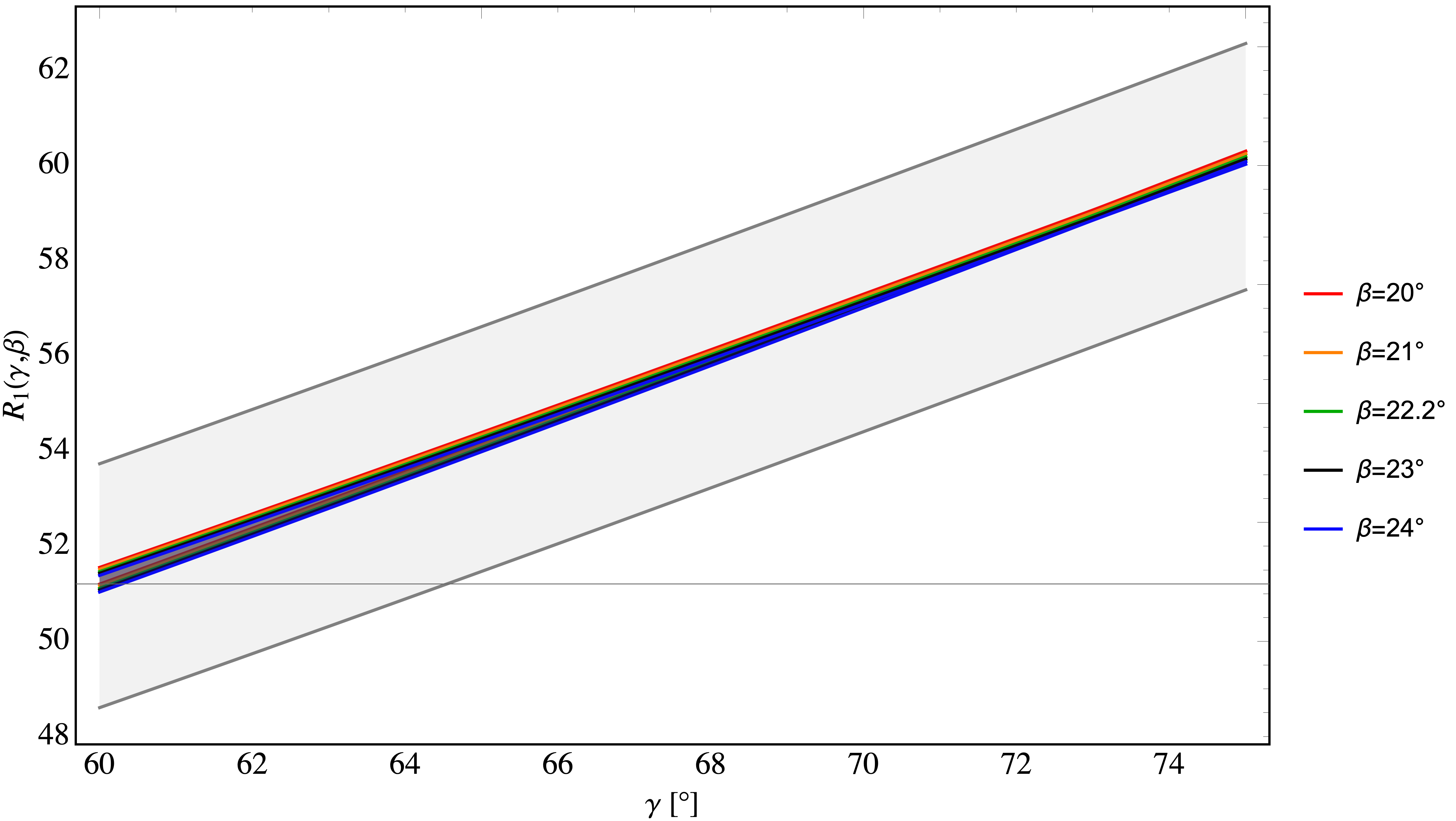
Figure 6: The ratios $R_{1}$ and $R_{2}$ defined in (45) as functions of $\gamma$ for different values of $\beta$ within the SM. The coloured bands correspond to $38<|V_{cb}|\times 10^{3}<43$, while the gray ones give the non-parametric uncertainties.

Figure 7: The correlations of $\mathcal{B}(K^{+}\rightarrow\pi^{+}\nu\bar{\nu})$ with $\overline{\mathcal{B}}(B_{s}\to\mu^{+}\mu^{-})^{1.4}$ (left panel) and with ${\mathcal{B}}(B_{d}\to\mu^{+}\mu^{-})^{1.4}$ (right panel) as given in (2.3) and (2.3), for different values of $\gamma$ within the SM. The ranges of branching ratios correspond to $38\leq|V_{cb}|\times 10^{3}\leq 43$ and $20^{\circ}\leq\beta\leq 24^{\circ}$. The gray area represents the present experimental situation.

Now, it is likely that the branching ratios for $K^{+}\rightarrow\pi^{+}\nu\bar{\nu}$ and $B_{s}\to\mu^{+}\mu^{-}$ will be measured accurately well ahead of the one for $B_{d}\to\mu^{+}\mu^{-}$ and waiting for the latter measurement the triple correlation between the three branching ratios will be useful. Improving on a similar correlation in [5] we find

$$\mathcal{B}(K^{+}\rightarrow\pi^{+}\nu\bar{\nu}) ={(7.92\pm 0.25)}\times 10^{-11}\left[\frac{\overline{\mathcal{B}}(B_{s}\to\mu^{+}\mu^{-})}{{3.47}\times 10^{-9}\bar{R}_{s}}\right]^{0.74}\left[\frac{{230.3}\text{MeV}}{F_{B_{s}}}\right]^{1.4}$$

$$\qquad\quad\times\left[\frac{\mathcal{B}(B_{d}\to\mu^{+}\mu^{-})}{{0.968}\times 10^{-10}\bar{R}_{d}}\right]^{0.74}\left[\frac{{190.0}\text{MeV}}{F_{B_{d}}}\right]^{1.4}\frac{H(\beta,\gamma)}{H(22.2^{\circ},67^{\circ})},$$ (47)

where

$$H(\beta,\gamma)=\frac{1}{(G(\beta,\gamma))^{1.4}}.$$ (48)

In Fig. 8 we show the $\gamma$ dependence of $H(\beta,\gamma)$ for $\beta=22.2^{\circ}$, which is very weak, implying a variation of less than $1\%$ for $H(\beta,\gamma)$ when $\gamma$ takes values in $[60^{\circ},75^{\circ}]$. The $\beta$ dependence is even weaker, less than $0.5\%$ for $\beta$ in $[20^{\circ},24^{\circ}]$ and it is not shown.

Figure 8: The function $H(\beta,\gamma)$ defined in (48) as functions of $\gamma$ for $\beta=22.2^{\circ}$.

Note that having in the future very accurate values for ${F_{B_{s}}}$, ${F_{B_{d}}}$ and the experimental branching ratios for $B_{s}\to\mu^{+}\mu^{-}$ and $K^{+}\rightarrow\pi^{+}\nu\bar{\nu}$ will allow to predict the branching ratio for $B_{d}\to\mu^{+}\mu^{-}$ with high precision in the SM practically without any dependence on CKM parameters due to the very weak dependence of $H(\beta,\gamma)$ on $\beta$ and $\gamma$.

Similarly, one can define $|V_{cb}|$-independent ratios

$$\boxed{R_{3}(\beta,\gamma)=\frac{\mathcal{B}(K_{L}\rightarrow\pi^{0}\nu\bar{\nu})}{\left[{\overline{\mathcal{B}}}(B_{s}\to\mu^{+}\mu^{-})\right]^{2}},\qquad R_{4}(\beta,\gamma)=\frac{\mathcal{B}(K_{L}\rightarrow\pi^{0}\nu\bar{\nu})}{\left[{\mathcal{B}}(B_{d}\to\mu^{+}\mu^{-})\right]^{2}}\,.}$$ (49)

$$R_{3}(\beta,\gamma)=\frac{{({2.17}\pm 0.09)}\times 10^{6}}{\bar{R}_{s}^{2}}\left[{\frac{\sin\gamma\sin\beta}{\sin(67^{\circ})\sin(22.2^{\circ})}}\right]^{2}\left[\frac{G(22.2^{\circ},67^{\circ})}{G(\beta,\gamma)}\right]^{4}\left(\frac{{230.3}\text{MeV}}{F_{B_{s}}}\right)^{4}\,,$$ (50)

$$R_{4}(\beta,\gamma)=\frac{{({2.79\pm 0.13})}\times 10^{9}}{\bar{R}_{d}^{2}}\left[{\frac{\sin(67^{\circ})}{\sin\gamma}\frac{\sin\beta}{\sin(22.2^{\circ})}}\right]^{2}\left(\frac{{190.0}\text{MeV}}{F_{B_{d}}}\right)^{4}.$$ (51)

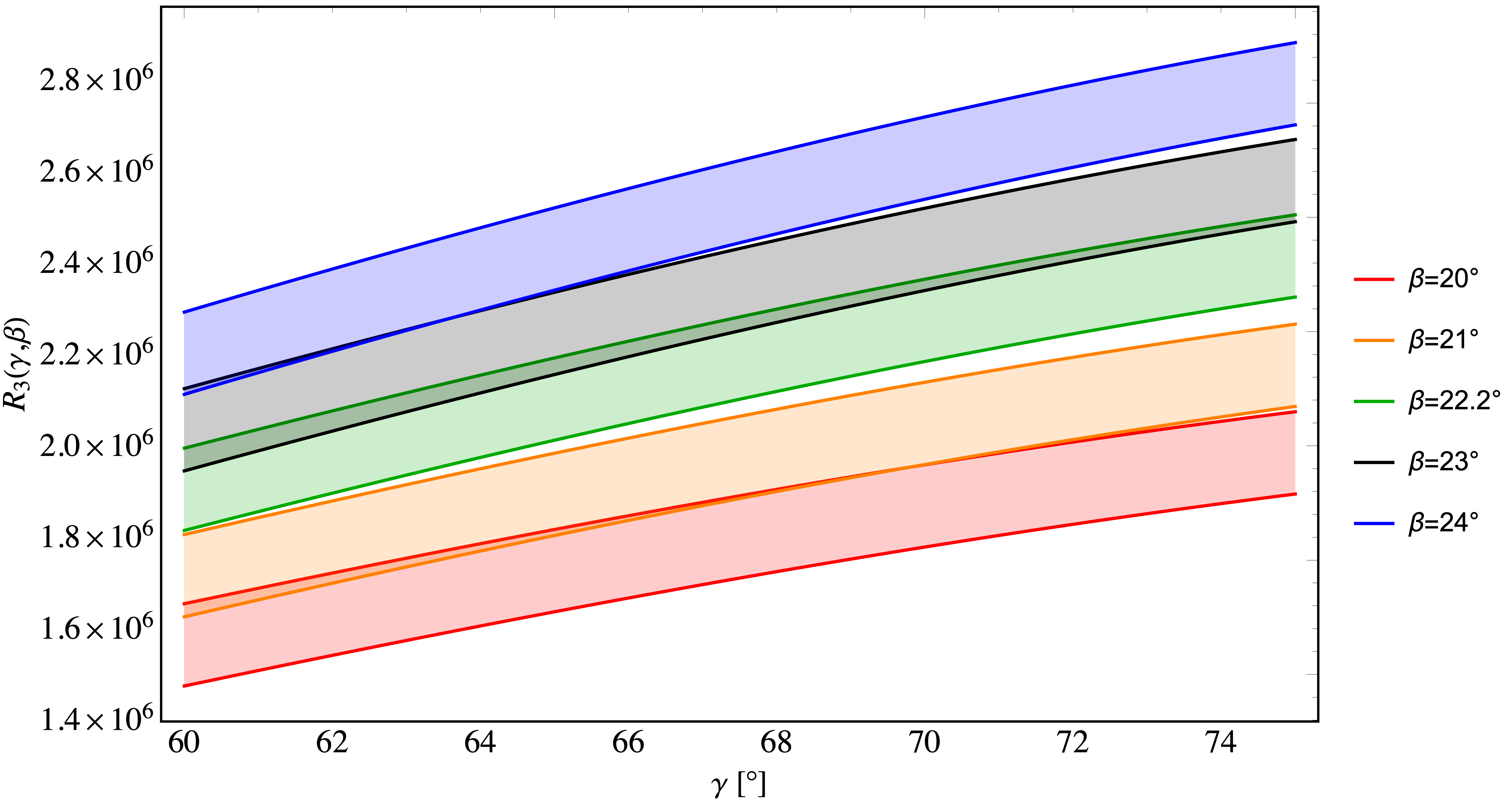
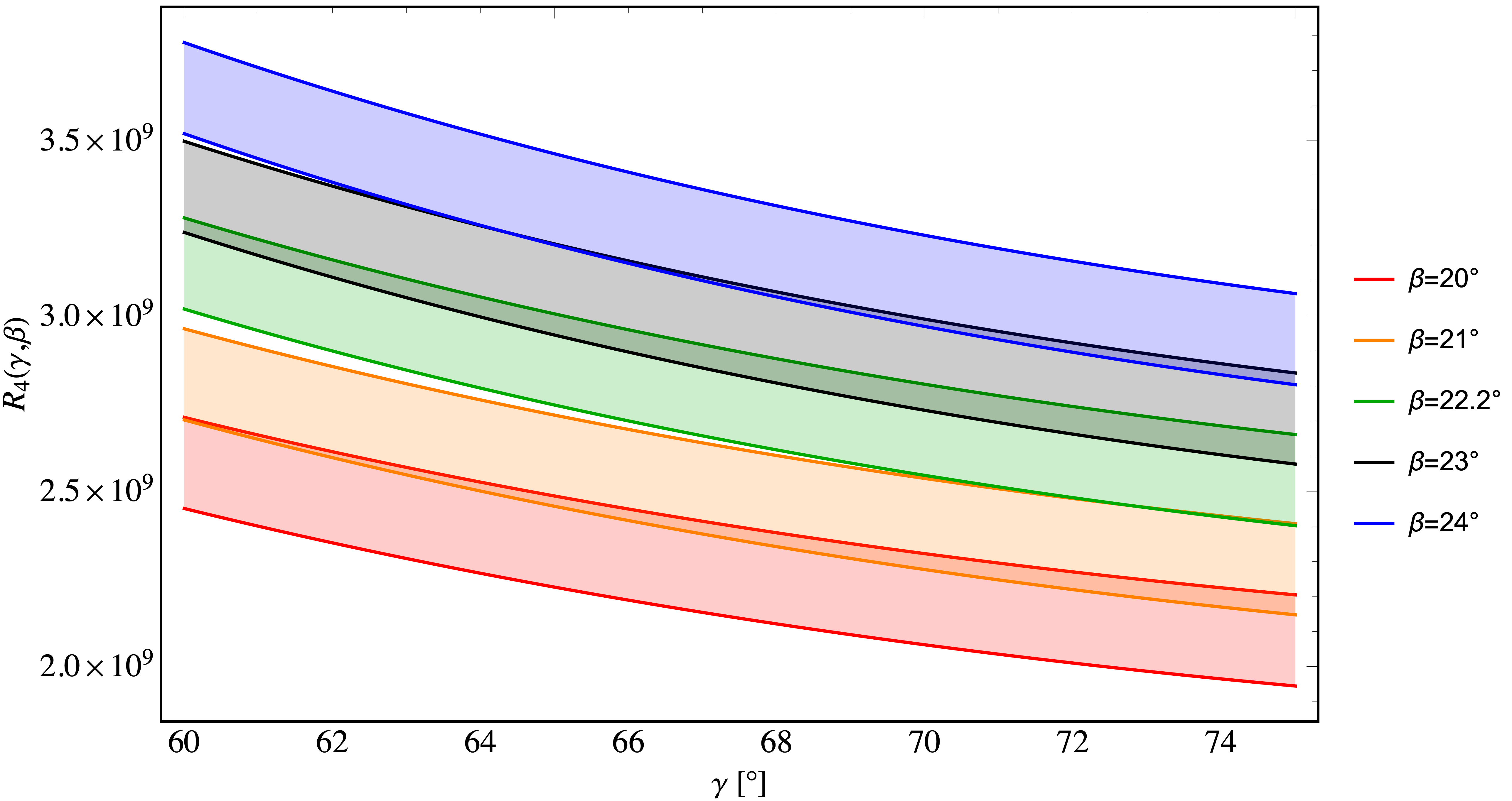
Figure 9: The ratios $R_{3}$ and $R_{4}$ as a functions of $\gamma$ for different values of $\beta$. The coloured bands represent the uncertainties associated to parameters different from $\gamma$ and $\beta$.

In Fig. 9 we show the ratios $R_{3}$ and $R_{4}$ as functions of $\gamma$ for different values of $\beta$. These plots have been obtained using the exact formulae for all branching ratios involved but almost the same results would we obtained by using the approximate expressions given above. In particular, the independence of these ratios from $|V_{cb}|$ is exact. One can notice that the uncertainty is dominated by the error on the $\gamma$ and $\beta$ angles, while the uncertainties associated with other parameters, depicted with coloured bands, are around one order of magnitude smaller.

2.4 Correlations with $B\to K^{*}\nu\bar{\nu}$ and $B\to K\nu\bar{\nu}$

The most recent SM estimate of the branching ratios for these decays, based on the formulae in [74] and the form factors in the case of $B\to K^{*}\nu\bar{\nu}$ from [75] and those for $B\to K\nu\bar{\nu}$ from [76] read

$${\mathcal{B}}(B^{+}\to K^{+}\nu\bar{\nu})_{\rm SM} =(4.18\pm 0.56)\times 10^{-6}\left|\frac{V_{ts}V_{tb}^{*}}{0.0402}\right|^{2},$$ (52)

$${\mathcal{B}}(B^{0}\to K^{0*}\nu\bar{\nu})_{\rm SM} =(9.08\pm 0.85)\times 10^{-6}\left|\frac{V_{ts}V_{tb}^{*}}{0.0402}\right|^{2},$$ (53)

which update those in [74].

Again the largest uncertainties in these branching ratios originate in the value of $|V_{cb}|$ which cancels out in the ratios

$$\boxed{R_{5}(\beta,\gamma)=\frac{\mathcal{B}(K^{+}\rightarrow\pi^{+}\nu\bar{\nu})}{\left[\mathcal{B}(B^{+}\to K^{+}\nu\bar{\nu})\right]^{1.4}},\qquad R_{6}(\beta,\gamma)=\frac{\mathcal{B}(K^{+}\rightarrow\pi^{+}\nu\bar{\nu})}{\left[\mathcal{B}(B^{0}\to K^{0*}\nu\bar{\nu})\right]^{1.4}}.}$$ (54)

We find then

$$R_{5}(\beta,\gamma)={(2.69\pm 0.51)}\times 10^{-3}\left[\frac{\sin\gamma}{\sin 67^{\circ}}\right]^{1.39}\left[\frac{G(22.2^{\circ},67^{\circ})}{G(\beta,\gamma)}\right]^{2.8},$$ (55)

$$R_{6}(\beta,\gamma)={(9.07\pm 1.23)}\times 10^{-4}\left[\frac{\sin\gamma}{\sin 67^{\circ}}\right]^{1.39}\left[\frac{G(22.2^{\circ},67^{\circ})}{G(\beta,\gamma)}\right]^{2.8}\,,$$ (56)

with $G(\beta,\gamma)$ defined in (14).

The ratios $R_{5}$ and $R_{6}$ are shown in Fig. 10 as functions of $\gamma$ for different values of $\beta$. We observe that their dependence on $\gamma$ and $\beta$ is the same as for $R_{1}$. In particular they are both nearly independent of $\beta$. The non-parametric uncertainties are fully dominated by formfactor uncertainties that should be significantly reduced in the coming years.

In Fig. 11 we show the correlations between $\mathcal{B}(K^{+}\rightarrow\pi^{+}\nu\bar{\nu})$ and $\mathcal{B}(B^{+}\to K^{+}\nu\bar{\nu})^{1.4}$ and between $\mathcal{B}(K^{+}\rightarrow\pi^{+}\nu\bar{\nu})$ and $\mathcal{B}(B^{0}\to K^{0*}\nu\bar{\nu})^{1.4}$. In both cases, the depicted linear relations are analogous to the one in the left panel of Fig. 7. Also these correlations are of interest for Belle II, NA62 and LHCb.

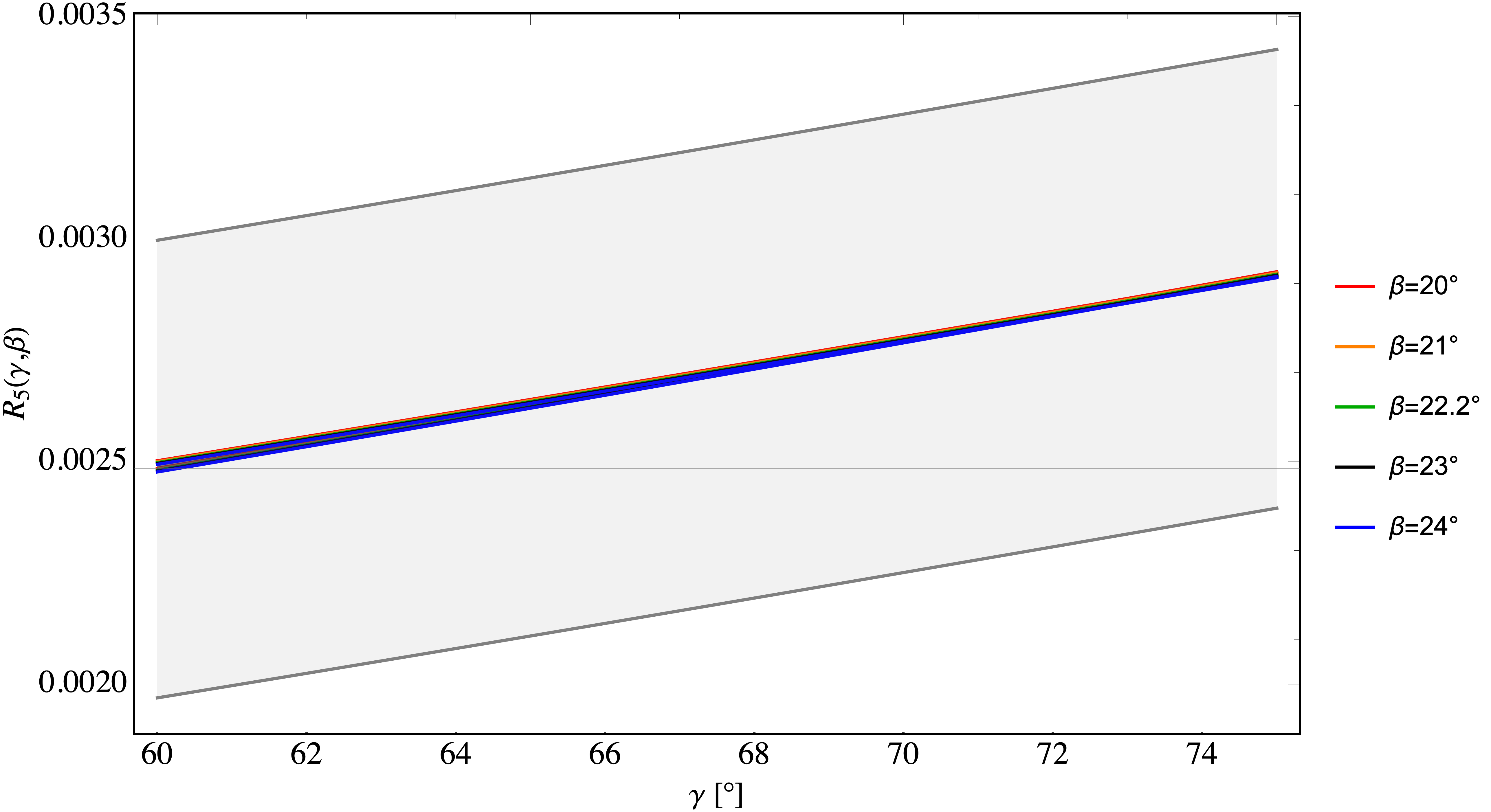
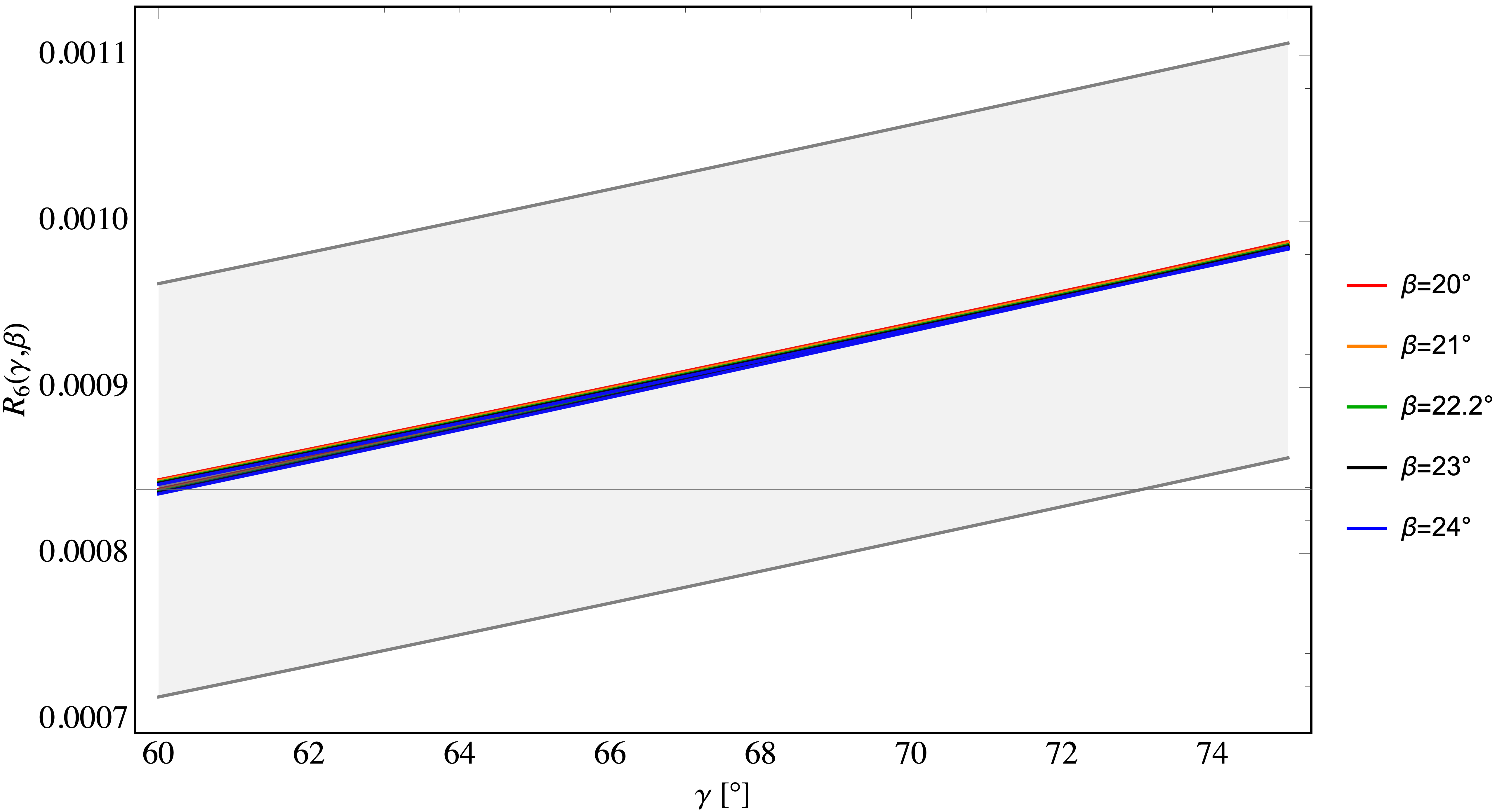
Figure 10: The ratios $R_{5}$ and $R_{6}$ as functions of $\gamma$ for different values of $\beta$. The coloured bands correspond to $38<|V_{cb}|\times 10^{3}<43$, while the gray ones give the non-parametric uncertainties.

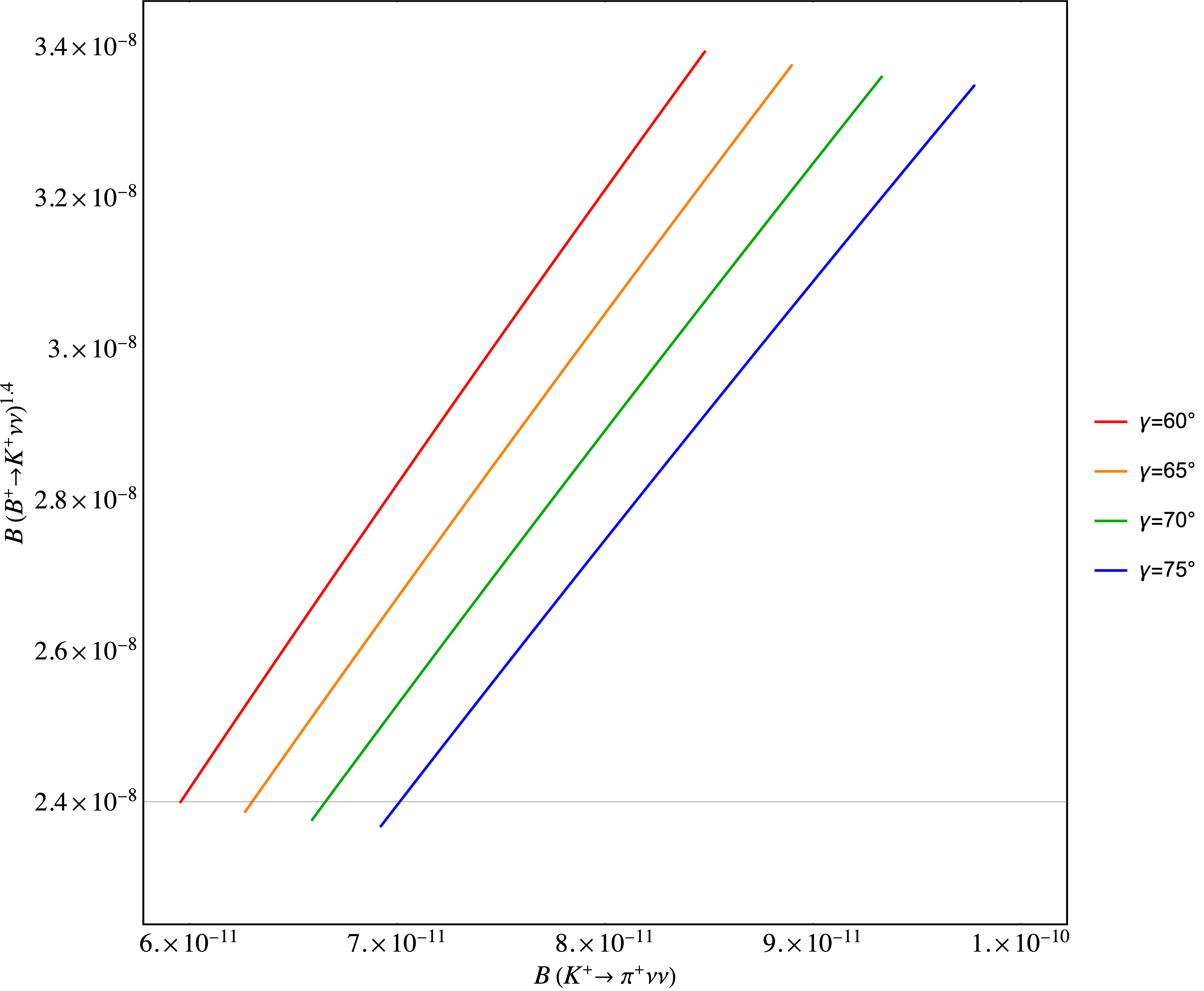
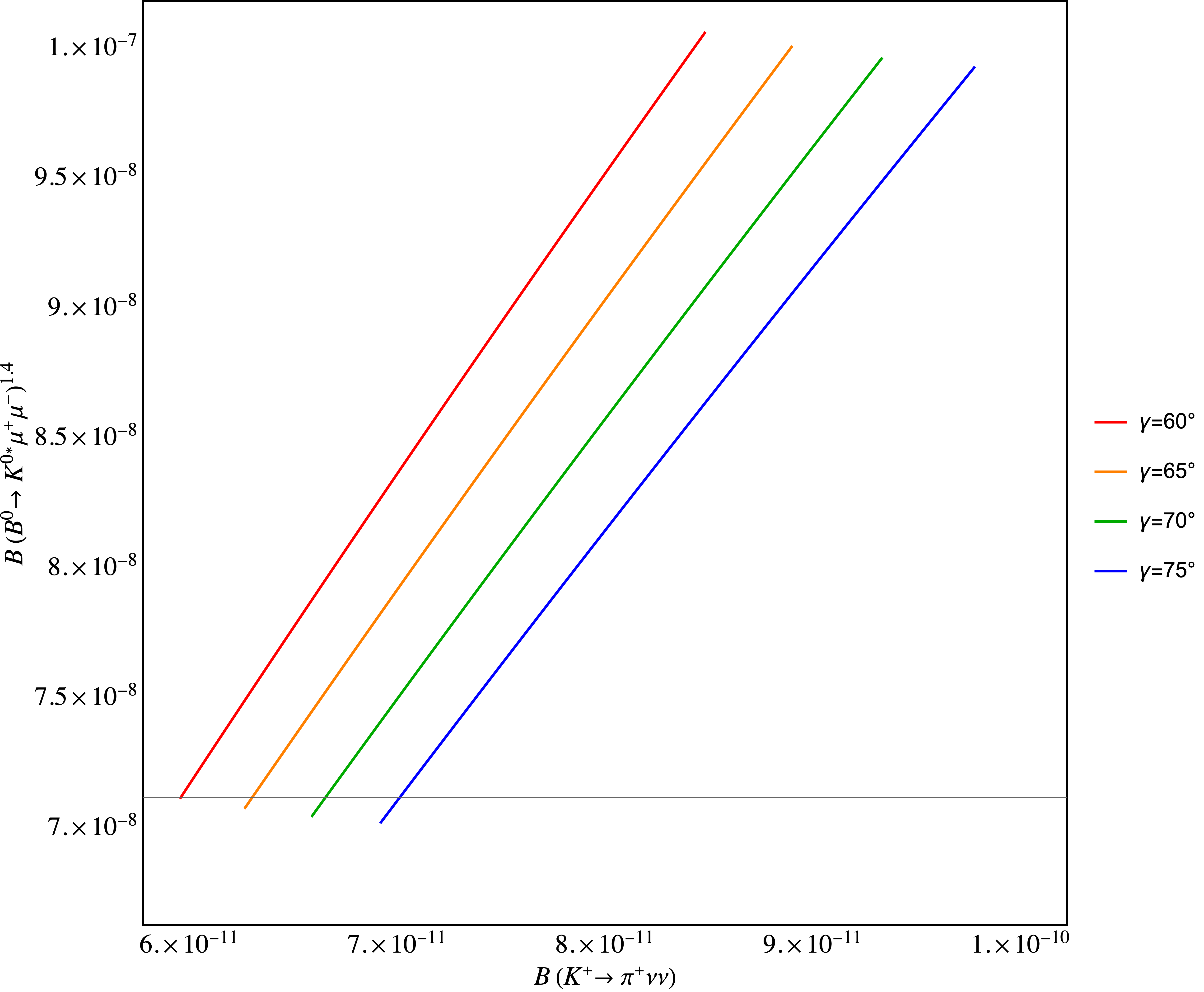
Figure 11: The correlations of $\mathcal{B}(K^{+}\rightarrow\pi^{+}\nu\bar{\nu})$ with $\mathcal{B}(B^{+}\to K^{+}\nu\bar{\nu})^{1.4}$ (left panel) and with $\mathcal{B}(B^{0}\to K^{0*}\nu\bar{\nu})^{1.4}$ (right panel) as given in (55) and (56), for different values of $\gamma$ within the SM. The ranges of branching ratios correspond to $38\leq|V_{cb}|\times 10^{3}\leq 43$ and $20^{\circ}\leq\beta\leq 24^{\circ}$.

Moreover, one has CKM-independent ratios

$$\boxed{R_{7}=\frac{\mathcal{B}(B^{+}\to K^{+}\nu\bar{\nu})}{{\overline{\mathcal{B}}}(B_{s}\to\mu^{+}\mu^{-})},\qquad R_{8}=\frac{\mathcal{B}(B^{0}\to K^{*0}\nu\bar{\nu})}{{\overline{\mathcal{B}}}(B_{s}\to\mu^{+}\mu^{-})}.}$$ (57)

Using (34) we find

$$(R_{7})_{\text{SM}}={({1.20}\pm 0.17)}\times 10^{3}\frac{1}{\bar{R}_{s}}\left(\frac{{230.3}\text{MeV}}{F_{B_{s}}}\right)^{2}\,,$$ (58)

$$(R_{8})_{\text{SM}}={({2.62}\pm 0.25)}\times 10^{3}\frac{1}{\bar{R}_{s}}\left(\frac{{230.3}\text{MeV}}{F_{B_{s}}}\right)^{2}\,.$$ (59)

Now the present world average experimental value from LHCb [71, 77], CMS [72, 78] and ATLAS [73, 79] as given in [70] and the preliminary result from Belle II [80] read respectively

$$\overline{\mathcal{B}}(B_{s}\to\mu^{+}\mu^{-})=(2.85\;{}^{+0.34}_{-0.31})\times 10^{-9}\,,\qquad\mathcal{B}(B^{+}\to K^{+}\nu\bar{\nu})=(11\pm 4)\times 10^{-6}\,$$ (60)

which implies

$$(R_{7})_{\rm EXP}=(3.86\pm 1.48)\times 10^{3}.$$ (61)

The central value is by a factor of 3.2 larger than the SM prediction (58) but due to large error in the experimental $B^{+}\to K^{+}\nu\bar{\nu}$ branching ratio the tension is only at $1.8\sigma$.

The origin of this significant discrepancy is the fact that whereas the central experimental value for $\mathcal{B}(B^{+}\to K^{+}\nu\bar{\nu})$ is by a factor of $2.5$ larger than the SM prediction, in the case of $\overline{\mathcal{B}}(B_{s}\to\mu^{+}\mu^{-})$, the data are by a factor of 1.3 below its SM value. While these factors correspond to $|V_{cb}|=42.0\times 10^{-3}$ and would both change with $|V_{cb}|$, the ratio $R_{7}$ is $|V_{cb}|$-independent.

The possible tension of Belle II data with the SM in the case of $\mathcal{B}(B^{+}\to K^{+}\nu\bar{\nu})$ has been pointed out first in [80] who found the data by a factor of $2.4\pm 0.9$ larger than its SM value estimate from [74] obtained with somewhat different formfactors than used by us here. However, this result corresponds to $|V_{cb}|=42.0\times 10^{-3}$ and the tension would increase for lower exclusive values of $|V_{cb}|$. In our approach the value of $|V_{cb}|$ does not matter.

3 $|V_{cb}|(\beta,\gamma)$ from $\varepsilon_{K}$, $\Delta M_{s}$ and $\Delta M_{d}$

3.1 Preliminaries

While the global analyses of the UT [81, 82] demonstrate good consistency of the SM with the data, in this section we want to have first a closer look at $\varepsilon_{K}$, $\Delta M_{s}$ and $\Delta M_{d}$ with the goal to check whether within the SM the same value of $|V_{cb}|$ allows to obtain for them simultaneously good agreement with the data and for which values of $\beta$ and $\gamma$ this turns out to be possible. This is analogous to the expressions in (23) and (38) but this time $|V_{cb}|$ is expressed in terms of precisely measured $\varepsilon_{K}$, $\Delta M_{s}$ and $\Delta M_{d}$ as opposed to rare decay branching ratios.

The motivation for this analysis comes from the fact that in the standard analysis of the UT the value of $|V_{cb}|$ remains hidden and only the angles $\beta$ and $\gamma$ are exposed. In this manner only two parameters among the four in (4) are visible. While $|V_{us}|$ plays totally subleading role in rare decays, the role of $|V_{cb}|$ is even more important than of $\beta$ and $\gamma$.

Therefore we want to propose here a test of the SM that is complementary to the usual UT-analyses. Namely, we propose to extract from a given observable the value of $|V_{cb}|$ as a function of $\beta$ and $\gamma$ for which the SM agrees with the experimental data. In what follows we will present this idea using $\varepsilon_{K}$, $\Delta M_{s}$ and $\Delta M_{d}$ for which both theory and experiment reached good precision but in the future other processes, in particular the theoretically clean rare decays considered by us, could also be used for this purpose when the experimental data improve

We will find that, while the dependence of $|V_{cb}|$ on $\beta$ and $\gamma$ extracted from $\varepsilon_{K}$ is rather rich, the one extracted from $\Delta M_{d}$ involves only $\gamma$. Finally, $|V_{cb}|$ extracted from $\Delta M_{s}$, is practically independent of both $\beta$ and $\gamma$. Our presentation begins therefore with $\varepsilon_{K}$ followed by the one on $\Delta M_{d}$ and $\Delta M_{s}$.

3.2 $|V_{cb}|(\beta,\gamma)$ from $\varepsilon_{K}$

In [25] a more accurate formula for $\varepsilon_{K}$ has been presented. It uses the unitarity relation $\lambda_{c}=-\lambda_{u}-\lambda_{t}$ instead of $\lambda_{u}=-\lambda_{c}-\lambda_{t}$ as done in the previous literature. This allows to remove significant theoretical uncertainties from charm contribution to $\varepsilon_{K}$. The new SM expression for $\varepsilon_{K}$ reads [25]

$$|\epsilon_{K}|=\kappa_{\epsilon}C_{\varepsilon}\hat{B}_{K}|V_{cb}|^{2}\lambda^{2}\bar{\eta}\times\Big{[}|V_{cb}|^{2}(1-\bar{\rho})\eta_{tt}S_{tt}(x_{t})-\eta_{ut}S_{ut}(x_{c},x_{t})\Big{]}\,.$$ (62)

It replaces the usual phenomenological expression given in [84]. Here

$$S_{tt}(x_{t})=S_{0}(x_{t})+S_{0}(x_{c})-2S_{0}(x_{c},x_{t}),\qquad S_{ut}(x_{c},x_{t})=S_{0}(x_{c})-S_{0}(x_{c},x_{t}),$$ (63)

where $S_{0}(x_{i})$ and $S_{0}(x_{i},x_{j})$ are the standard Inami-Lim functions [85, 86] with explicit expressions given in Appendix A.

The QCD factors in (62) at the NLO and NNLO level, respectively, read [25]

$$\eta_{tt}=0.55(2),\qquad\eta_{ut}=0.402(5).$$ (64)

Next, the kaon bag parameter comprising the hadronic matrix element of the local $\Delta S=2$ operators is given by $\hat{B}_{K}=0.7625(97)$ [46]. The phenomenological parameter $\kappa_{\epsilon}=0.94(2)$ [48] comprises long-distance contributions beyond the lowest order in the operator-product expansion, which are not included in $\hat{B}_{K}$.

Finally,

$$C_{\varepsilon}=\frac{G_{F}^{2}F_{K}^{2}m_{K^{0}}M_{W}^{2}}{6\sqrt{2}\pi^{2}(\Delta M_{K})_{\rm exp}}={3.635\times 10^{4}.}$$ (65)

The new expression in (62) is significantly more accurate than the old one as far as theoretical uncertainties are concerned but it is still subject to large uncertainty due to $|V_{cb}|$.

Defining then

$$r_{1}=\frac{1}{(1-\bar{\rho})}\frac{\eta_{ut}S_{ut}(x_{c},x_{t})}{\eta_{tt}S_{tt}(x_{t})},\quad r_{2}=\kappa_{\epsilon}C_{\varepsilon}\hat{B}_{K}\lambda^{2}\bar{\eta}(1-\bar{\rho})\eta_{tt}S_{tt}(x_{t}),$$ (66)

we find

$$\boxed{|V_{cb}|^{2}=\frac{1}{2}\left[r_{1}+\sqrt{r^{2}_{1}+4\frac{|\epsilon_{K}|}{r_{2}}}\right]}$$ (67)

with $\bar{\rho}$ and $\bar{\eta}$ being through (12) functions of $\beta$ and $\gamma$. In this manner one of the basic parameters in (4), namely $|V_{cb}|$, has been traded for $|\epsilon_{K}|$ that is very precisely measured. Surprisingly, to our knowledge this expression for $|V_{cb}|$ in terms of $\beta$, $\gamma$ and $|\epsilon_{K}|$ has never been presented in the literature.

Choosing the central experimental value for $|\epsilon_{K}|$ in Table 1 and the reference values in (16) ($\lambda=0.225$, $\gamma=67^{\circ}$ and $\beta=22.2^{\circ}$) we find $|V_{cb}|=42.2\times 10^{-3}$ that favours the inclusive determinations of this parameter. The full $\beta$ and $\gamma$ dependence of $|V_{cb}|$ following from $(\ref{vcb2})$ is shown in Fig. 12. The green band corresponds to the $1\sigma$ range for $\beta$ determined from $S_{\psi K_{S}}=0.699(17)$:

$$21.5^{\circ}\leq\beta\leq 22.9^{\circ}\,.$$ (68)

We will see soon that this is an important constraint. Before describing this result in detail let us extract first $|V_{cb}|$ from $\Delta M_{d}$ and $\Delta M_{s}$.

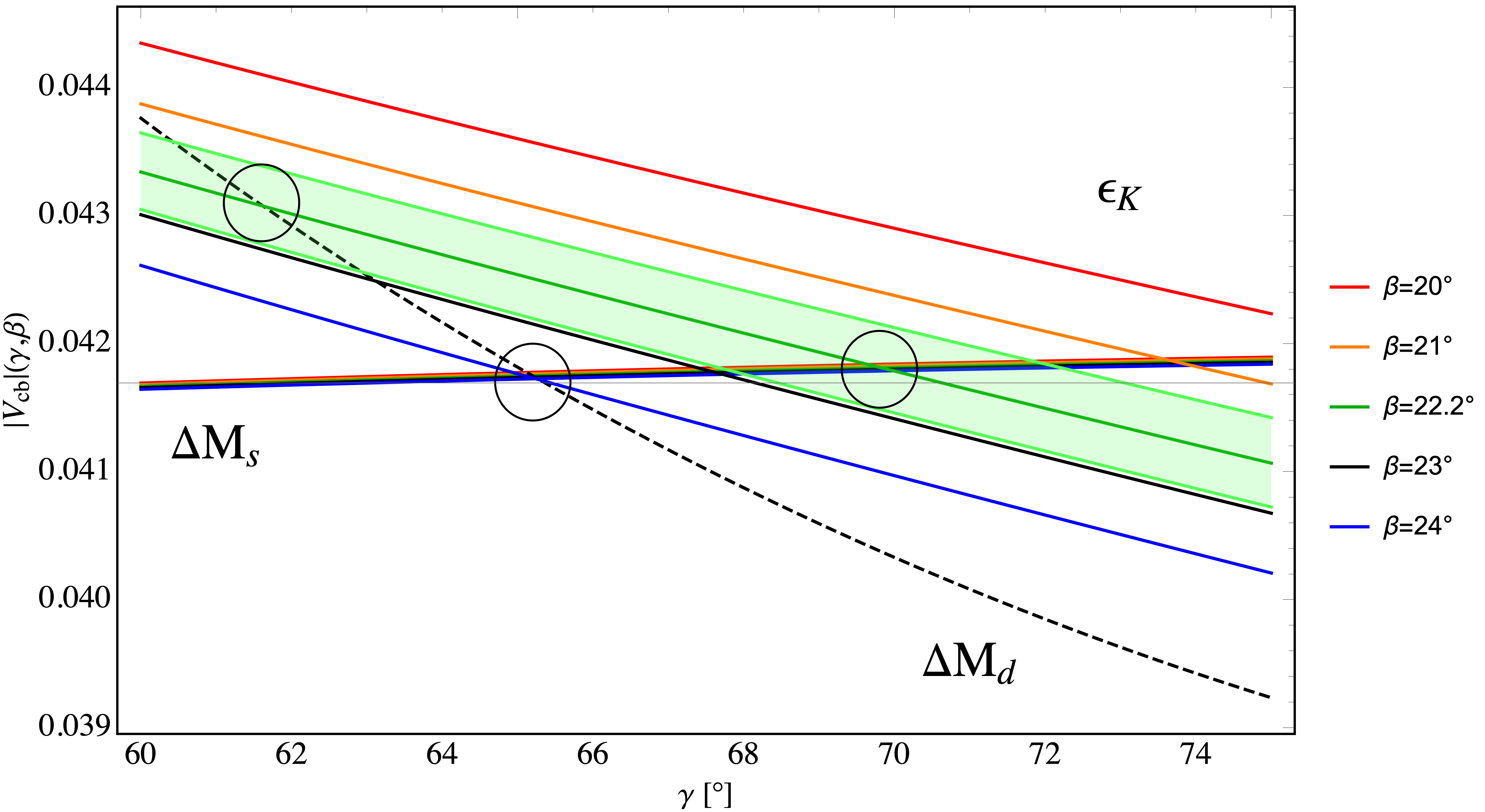
Figure 12: The values of $|V_{cb}|$ extracted from $\varepsilon_{K}$, $\Delta M_{d}$ and $\Delta M_{s}$ as functions of $\gamma$ for different values of $\beta$. $|V_{cb}|$ extracted from $\Delta M_{d}$ is independent of $\beta$.

3.3 $|V_{cb}|(\beta,\gamma)$ from $\Delta M_{d}$ and $\Delta M_{s}$

Updating the two very accurate formulae from [37] we have:

$$\Delta M_{d} = 0.5065/{\rm ps}\times\left[\frac{\sqrt{\hat{B}_{B_{d}}}F_{B_{d}}}{214.0\text{MeV}}\right]^{2}\left[\frac{S_{0}(x_{t})}{2.307}\right]\left[\frac{|V_{td}|}{8.53\times 10^{-3}}\right]^{2}\left[\frac{\eta_{B}}{0.5521}\right]\,,$$ (69)

$$\Delta M_{s} = 17.749/{\rm ps}\times\left[\frac{\sqrt{\hat{B}_{B_{s}}}F_{B_{s}}}{261.7\text{MeV}}\right]^{2}\left[\frac{S_{0}(x_{t})}{2.307}\right]\left[\frac{|V_{ts}|}{41.0\times 10^{-3}}\right]^{2}\left[\frac{\eta_{B}}{0.5521}\right]\,.$$ (70)

The value $2.307$ in the normalization of $S_{0}(x_{t})$ is its SM value for $m_{t}(m_{t})=162.83\,\text{GeV}$. The central values of $|V_{td}|$ and $|V_{ts}|$ exposed here are chosen to make the overall factors in these formulae to be equal to the experimental values of the two observables. One can check that, for $\gamma=67^{\circ}$ and $\beta=22.2^{\circ}$, these values of $|V_{td}|$ and $|V_{ts}|$ correspond to $|V_{cb}|=41.2\times 10^{-3}$ and $|V_{cb}|=41.8\times 10^{-3}$, respectively. See Table 1 for other parameters.

The measurement of $\Delta M_{d}$ together with $\Delta M_{s}$ allows to determine $R_{t}$ or equivalently $\gamma$ without any dependence on $m_{t}$ and $|V_{cb}|$. To an excelent approximation one finds [37]

$$\frac{|V_{td}|}{|V_{ts}|}=\xi\sqrt{\frac{m_{B_{s}}}{m_{B_{d}}}}\sqrt{\frac{\Delta M_{d}}{\Delta M_{s}}}\quad\Longrightarrow\quad\sin\gamma={0.750}\,\xi,\qquad\xi=\frac{\sqrt{\hat{B}_{B_{s}}}F_{B_{s}}}{\sqrt{\hat{B}_{B_{d}}}F_{B_{d}}}$$ (71)

where $\beta=22.2^{\circ}$, corresponding to $S_{\psi K_{S}}=0.699$ has been used. But the dependence on $\beta$ is very weak as one can check using the expressions in (13) and (14) so that this relation is an excellent approximation for the full range of $\beta$ used by us.

This determination of $\gamma$ can be confronted with the tree-level determination of $\gamma$ with the help of non-leptonic two-body decays as mentioned before. As the mass differences $\Delta M_{s,d}$ are very precisely measured, the $\gamma$ following from their ratio depends as seen in (71) to an excellent approximation solely on $\xi$. This dependence is shown in Fig. 3 of [37].

Now, various LQCD collaborations contributed to the evaluation of $\xi$. In particular Fermilab-MILC collaboration [91] with $\xi=1.206\pm 0.019$ and RBC-UKQCD collaboration with $\xi=1.1853\pm 0.0054^{+0.0116}_{-0.0156}$ [92]. Similar value has been obtained from HQET sum rules: $\xi=1.2014^{+0.0065}_{-0.0072}$ [93]. With these values $\gamma$ is found in the range $60^{\circ}\leq\gamma\leq 65^{\circ}$. In particular the present value of $\gamma$ corresponding to the FLAG average for $\xi$ reads [46]

$$\xi=1.206(17),\qquad\gamma=64.7(16)^{\circ}.$$ (72)

Until recently the central values for $\gamma$ from the LHCb collaboration were in the ballpark of $74^{\circ}$ implying in particular some tension between the FLAG value and the one from non-leptonic decays pointed out in [37]. However the most recent LHCb value in (5) is in a good agreement with (72).

But as the error on $\gamma$ from LHCb is still large let us have a closer look and determine within the SM $|V_{cb}|$ independently from $\Delta M_{d}$ and $\Delta M_{s}$. Using (69) and (70) together with (13) and (14) we find

$$|V_{cb}|=\frac{{8.53}\times 10^{-3}}{\lambda\sin\gamma}\left[\frac{214.0\text{MeV}}{\sqrt{\hat{B}_{B_{d}}}F_{B_{d}}}\right],\qquad(\Delta M_{d}),$$ (73)

$$|V_{cb}|=\frac{{41.0}\times 10^{-3}}{G(\beta,\gamma)}\left[\frac{261.7\text{MeV}}{\sqrt{\hat{B}_{B_{s}}}F_{B_{s}}}\right],\qquad(\Delta M_{s}).$$ (74)

with $G(\beta,\gamma)$ defined in (14). For the reference values in (16) ($\lambda=0.225$, $\gamma=67^{\circ}$ and $\beta=22.2^{\circ}$) we find $|V_{cb}|=41.2\times 10^{-3}$ and $|V_{cb}|=41.8\times 10^{-3}$, respectively. While the experimental errors coming from the $\Delta M_{d}$ and $\Delta M_{s}$ measurements can be safely neglected, the theoretical errors associated to the uncertainties on the $\sqrt{\hat{B}_{B_{d,s}}}F_{B_{d,s}}$ factors induce errors respectively of $1.8\%$ and of $1.5\%$ on the corresponding $|V_{cb}|$ determinations. These uncertainties are not shown in the figures, for the sake of readability.

In Fig. 12 we show $|V_{cb}|$ as given above as function of $\gamma$ for different values of $\beta$ and compare it with the one obtained from $\varepsilon_{K}$.

We observe that

• $|V_{cb}|$ extracted from $\varepsilon_{K}$ shows significant dependence on both $\beta$ and $\gamma$.

• $|V_{cb}|$ extracted from $\Delta M_{d}$ is independent of $\beta$ but shows a significant dependence on $\gamma$ which is evident from the expression in (73).

• $|V_{cb}|$ extracted from $\Delta M_{s}$ is practically independent of both $\beta$ and $\gamma$ because the element $|V_{ts}|$ governing $\Delta M_{s}$ differs from $|V_{td}|$ only by the function $G(\beta,\gamma)$ which is weakly dependent on both angles of the UT.

Therefore the last finding implies that just on the basis of $\Delta M_{s}$ alone a rather precise value of $|V_{cb}|$ can be obtained. Considering the full range of $\gamma$ and $\beta$ and the error on $\sqrt{\hat{B}_{B_{s}}}F_{B_{s}}$ in Table 1 we find

$$\boxed{|V_{cb}|={41.78(62)}\times 10^{-3},\qquad(\Delta M_{s})\,}$$ (75)

where the largest contribution to the error, ${0.61}\times 10^{-3}$, is due to the uncertainty on $\sqrt{\hat{B}_{B_{s}}}F_{B_{s}}$. This result agrees very well with the one obtained using HQET sum rules [94].

In view of the strong dependence of $\varepsilon_{K}$ and $\Delta M_{d}$ on $\gamma$ which is presently not precisely known and the persistent tension between inclusive and exclusive determinations of $|V_{cb}|$ we point out that presently the result in (75) is the most precise determination of this CKM element based on a single quantity. We impose, then, the constraint on $\beta$ coming from $S_{\psi K_{S}}$, i.e. $\beta=22.2(7)^{\circ}$, and on $\gamma$ coming from $\varepsilon_{K}$, that together with $\Delta M_{s}$ implies $\gamma=69.8(26)^{\circ}$ for $\beta$ varying in its $S_{\psi K_{S}}$ range; the obtained $|V_{cb}|$ becomes

$$\boxed{|V_{cb}|=41.{81(61)}\times 10^{-3},\qquad(\Delta M_{s}\,,~{}|\varepsilon_{K}|,~{}S_{\psi K_{S}}).}$$ (76)

The question then arises what happens when also $\Delta M_{d}$ is taken into account and what these results imply for $\gamma$. To this end let us note the following pattern implied by Fig. 12.

• The values of $\beta$, $\gamma$ and $|V_{cb}|$ following simultaneously from $\varepsilon_{K}$, $\Delta M_{s}$ and $\Delta M_{d}$ are

  $$\boxed{\beta=24.0(14)^{\circ},\qquad\gamma=65.2(28)^{\circ},\qquad|V_{cb}|=41.7(6)\times 10^{-3}}\,.$$ (77)

  While the value of $\gamma$ is consistent with the FLAG determination in (72), the value of $\beta$ is outside the 1$\sigma$ range in (5) and would imply $S_{\psi K_{S}}=0.743$. This tension could be cured by a NP phase $\phi_{\rm NP}$ in the ballpark of $-2^{\circ}$

  $$S_{\psi K_{S}}=\sin(2\beta+2\phi_{\rm NP})\,.$$ (78)

  The error on $\beta$ determined in this manner, being twice as large as the one from $S_{\psi K_{S}}$, demonstrates clearly the virtue of the determination of $\beta$ by means of the latter asymmetry.

• Imposing then $\beta=22.2(7)^{\circ}$, from the $S_{\psi K_{S}}$ measurement, we find from $\varepsilon_{K}$ and $\Delta M_{d}$

  $$\boxed{\beta=22.2{(7)}^{\circ},\qquad\gamma=61.6(16)^{\circ},\qquad|V_{cb}|=43.{1(10)}\times 10^{-3}}\,.$$ (79)

  This time $\gamma$ is below FLAG determination and $|V_{cb}|$ is even larger than its inclusive determinations.

• On the other hand from $\varepsilon_{K}$ and $\Delta M_{s}$ we find

  $$\boxed{\beta=22.2{(7)}^{\circ},\qquad\gamma=69.{8(26)}^{\circ},\qquad|V_{cb}|=41.8{(6)}\times 10^{-3}}\,.$$ (80)

  This is precisely the case leading to (76); the corresponding value of $\gamma$ is this time significantly larger than the one from FLAG in (72) but consistent with the LHCb value in (5) due to its large error.

These three cases are nicely depicted by three circles in Fig. 12. There is no question about that there are some tensions between these three determinations visible in the plot but this requires simultaneous determination of $\beta$ from $S_{\psi K_{S}}$

. It is evident from this plot how important will be future determinations of $\gamma$ from LHCb and Belle II.

The values of $|V_{cb}|$ in these three cases can be compared with the values quoted by PDG obtained using CKMfit and UTfit prescriptions. They are $|V_{cb}|=40.5(8)\times 10^{-3}$ and $|V_{cb}|=42.0(6)\times 10^{-3}$, respectively. As both collaborations determine practically the same central value of $\gamma=68.7^{\circ}$, the resulting central values of the branching ratios for $K^{+}\rightarrow\pi^{+}\nu\bar{\nu}$ being $7.9\times 10^{-11}$ and $8.7\times 10^{-11}$ exhibit the $|V_{cb}|$-problem in question that affects global fits.

Having the results for $|V_{cb}|$ in Fig. 12 at hand we can use the relation in (13) to obtain analogous results for $|V_{ub}|$. They are shown in Fig.  13. They should be compared with [46]

$$|V_{ub}|=3.73(14)\times 10^{-3},\qquad{(\rm FLAG)},$$ (81)

which are indicated by gray bands in the three plots in this figure. We observe that $|V_{ub}|$ extracted from any of the three observables has almost the same dependence on $\beta$, dominated by the $\sin\beta$ factor in the ratio between $|V_{ub}|$ and $|V_{cb}|$. It is stronger with respect to the dependence on $\gamma$, especially in the case of $\epsilon_{K}$ and $\Delta M_{s}$, where $|V_{ub}|$ is almost $\gamma$ independent. But the main message from the plot is the agreement with the FLAG value above for $\beta$ from $S_{\psi K_{S}}$. In this manner, the inclusive determinations of $|V_{ub}|$ with central values being above $0.0040$ are practically excluded.

In view of this result it is tempting to calculate $|V_{ub}|$ corresponding to $|V_{cb}|$ in (76). We find

$$\boxed{|V_{ub}|=3.65(12)\times 10^{-3},\qquad(\Delta M_{s}\,,~{}|\varepsilon_{K}|,~{}S_{\psi K_{S}}),}$$ (82)

in good agreement with the FLAG’s value in (81) and also with $|V_{ub}|=3.77(15)\times 10^{-3}$ from light-cone sum rules [95].

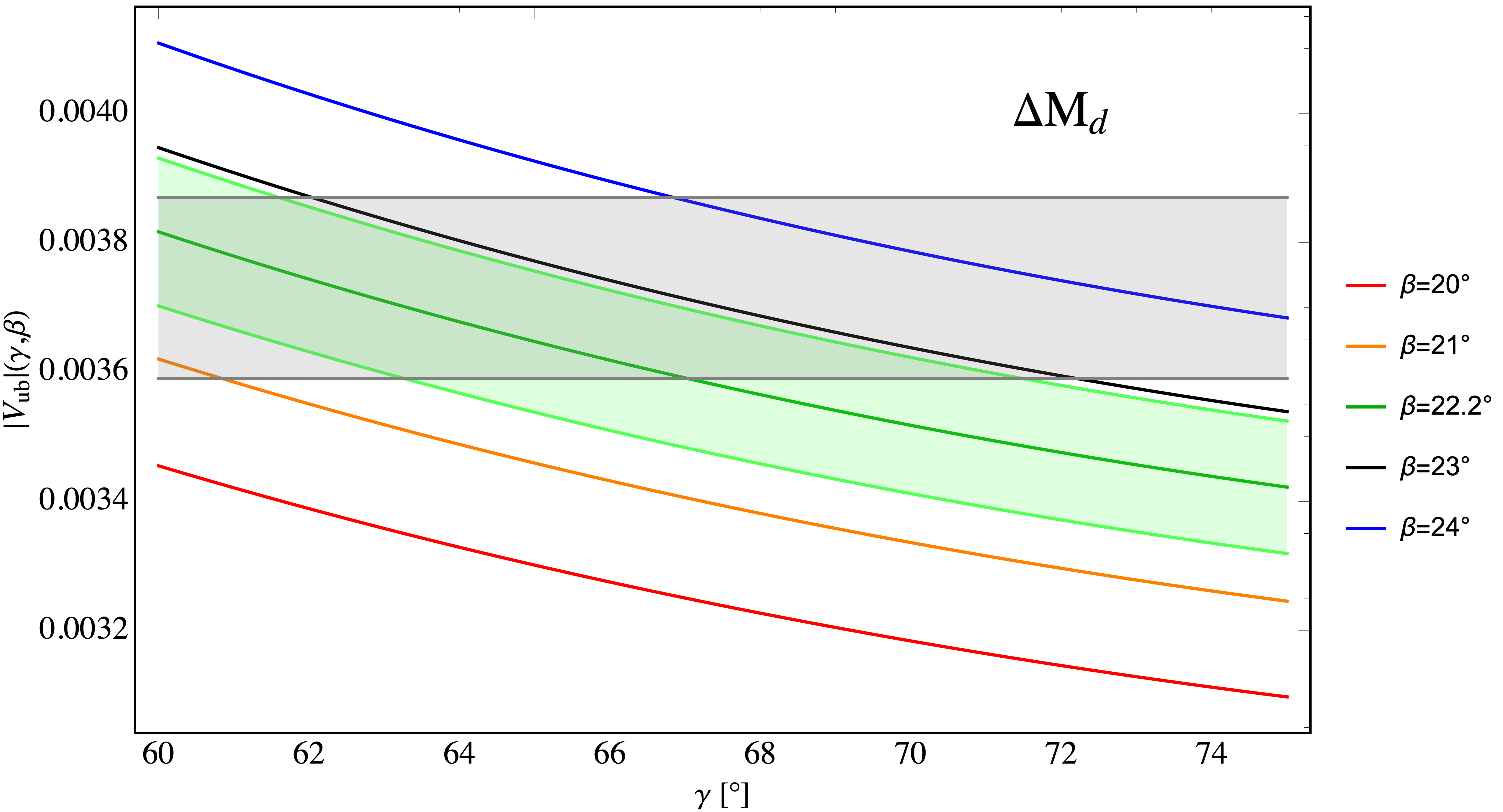
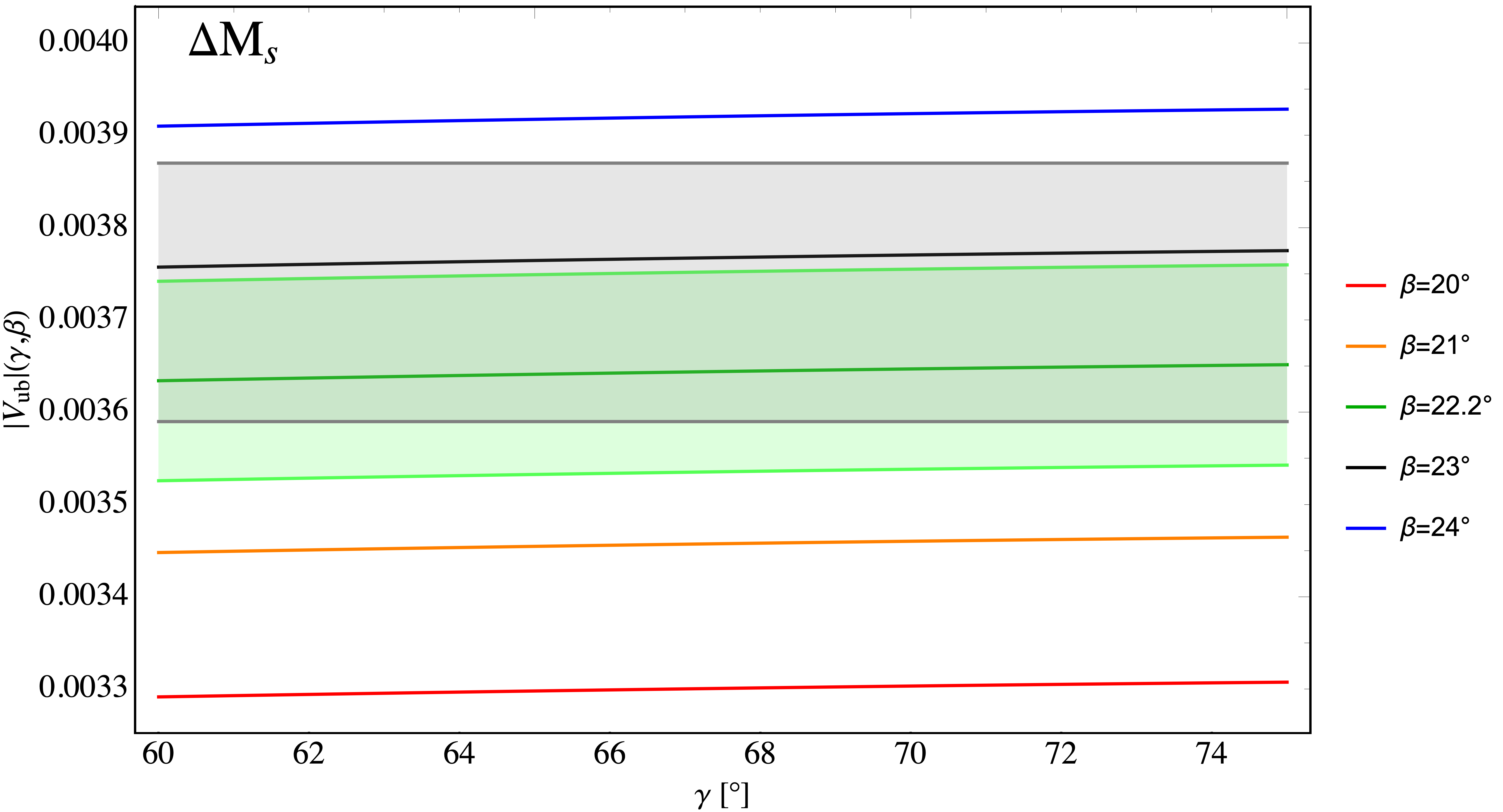
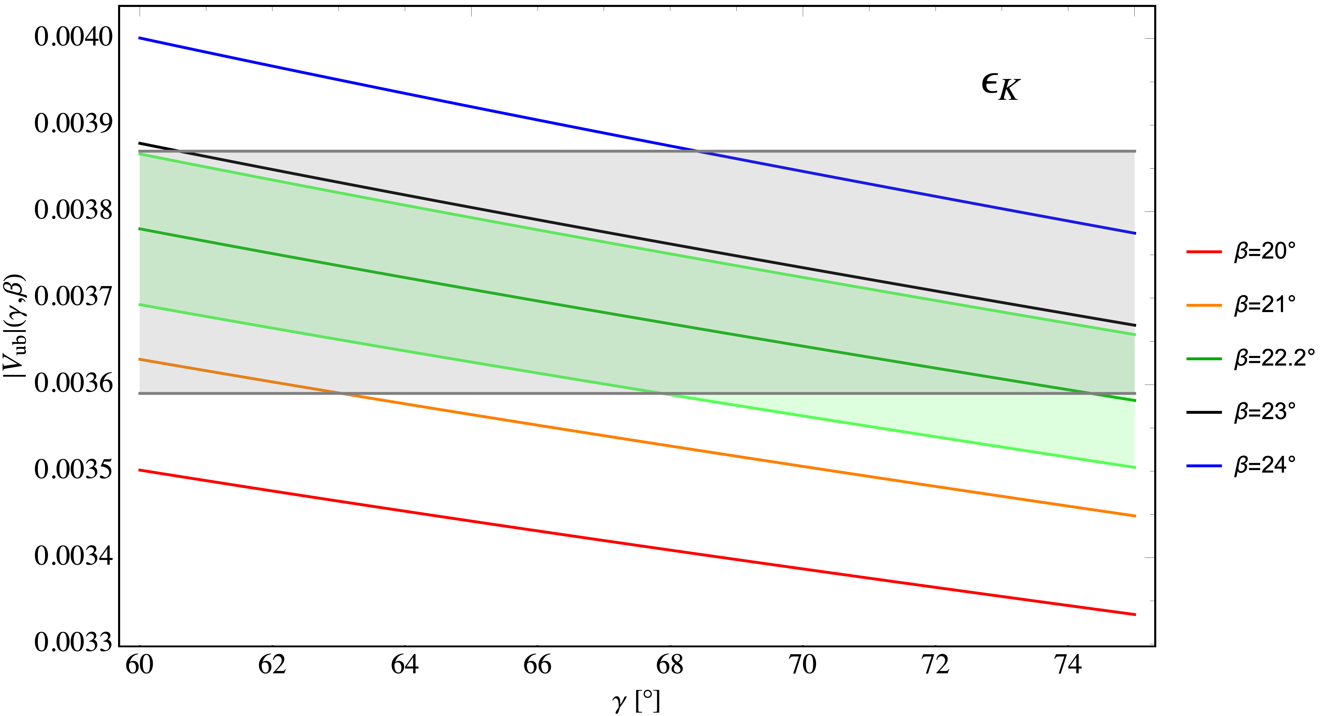
Figure 13: The values of $|V_{ub}|$ extracted from $\Delta M_{s}$, $\Delta M_{d}$ and $\varepsilon_{K}$ as functions of $\gamma$ for different values of $\beta$. The gray bands represent the FLAG measurement.

While the interplay between $\varepsilon_{K}$, $\Delta M_{d}$, $\Delta M_{s}$, $\beta$, $\gamma$, $|V_{ub}|$ and $|V_{cb}|$ has been discussed already in a number of papers in the past [96, 84, 37, 28], our presentations in Figs. 12 and 13 are new. But also in these papers some tension between these observables within the SM have been found. In particular in [28] it has been pointed out that with $\gamma$ in the ballpark of $74^{\circ}$, as signalled by the LHCb collaboration in 2018, and $|V_{cb}|$ determined from inclusive decays the SM value for $\Delta M_{d}$ was significantly above the data while $\varepsilon_{K}$ within the SM was consistent with the data. These finding can be confirmed by inspecting our plots and setting $\gamma=74^{\circ}$. In particular in this case FLAG and LHCb values for $\gamma$ disagree with each other.

In the meantime the most recent LHCb value in (5) seems to agree well with the FLAG value in (72) and the situation changed relative to the one addressed in [28]. Yet, as we have seen, some tensions remained but in contrast to the latter paper we want to address the possible tension between $\varepsilon_{K}$ and $\Delta M_{d}$ and even $\Delta M_{s}$ in the spirit of the present paper, that is in the $|V_{cb}|$-independent manner.

To this end we cast the formula (62) in a form analogous to (21) to find

$$|\varepsilon_{K}|={2.015\times 10^{-3}\times\left(\frac{V_{cb}}{41.0\times 10^{-3}}\right)^{3.4}\left(\frac{\sin\gamma}{\sin 67^{\circ}}\right)^{1.67}\left(\frac{\sin\beta}{\sin 22.2^{\circ}}\right)^{0.87}}$$ (83)

where the central value has been evaluated with (62), using the numerical values given in Section 3.2. The expression above provides an approximation of (62) with an accuracy of 1.5%, in the ranges $38<|V_{cb}|\times 10^{3}<43$, $60^{\circ}<\gamma<75^{\circ}$, $20^{\circ}<\beta<24^{\circ}$.

We consequently define two $|V_{cb}|$-independent ratios

$$\boxed{R_{9}(\beta,\gamma)=\frac{|\varepsilon_{K}|}{(\Delta M_{d})^{{1.7}}},\qquad R_{10}(\beta,\gamma)=\frac{|\varepsilon_{K}|}{(\Delta M_{s})^{{1.7}}}\,.}$$ (84)

The explicit expressions for them read

$${R_{9}(\beta,\gamma)=6.405\times 10^{-3}\,{\rm ps^{1.7}}\left(\frac{\sin 67^{\circ}}{\sin\gamma}\right)^{1.73}\left(\frac{\sin\beta}{\sin 22.2^{\circ}}\right)^{0.87}\bar{R}^{\epsilon}_{d}},$$ (85)

$${R_{10}(\beta,\gamma)=1.516\times 10^{-5}\,{\rm ps^{1.7}}\left(\frac{\sin\gamma}{\sin 67^{\circ}}\right)^{1.67}\left(\frac{\sin\beta}{\sin 22.2^{\circ}}\right)^{0.87}\left(\frac{G(22.2^{\circ},67^{\circ})}{G(\beta,\gamma)}\right)^{3.4}\bar{R}^{\epsilon}_{s}}$$ (86)

where

$$\bar{R}^{\epsilon}_{d}=\left(\frac{214.0\text{MeV}}{\sqrt{\hat{B}_{B_{d}}}F_{B_{d}}}\right)^{3.4}\left(\frac{2.307}{S_{0}(x_{t})}\right)^{1.7}\left(\frac{0.5521}{\eta_{B}}\right)^{1.7}\,,$$ (87)

$$\bar{R}^{\epsilon}_{s}=\left(\frac{261.7\text{MeV}}{\sqrt{\hat{B}_{B_{s}}}F_{B_{s}}}\right)^{3.4}\left(\frac{2.307}{S_{0}(x_{t})}\right)^{1.7}\left(\frac{0.5521}{\eta_{B}}\right)^{1.7}\,.$$ (88)

The ratios $R_{9}$ and $R_{10}$ are shown in Fig. 14 as functions of $\gamma$ for different values of $\beta$. One can see that, indeed, the dependence of these two ratios on $|V_{cb}|$ is very mild, with a variation only of $\lesssim 0.5\%$ for $38<|V_{cb}|\times 10^{3}<43$. On the other hand their experimental values are very precise and read

$$R_{9}=7.082(42)\times 10^{-3}{\rm ps^{1.7}},\qquad R_{10}=1.676(8)\times 10^{-5}{\rm ps^{1.7}}\,.$$ (89)

They are shown in Fig. 14 as very thin horizontal lines. The circles correspond to the ones in Fig. 12. But now the dependence on $|V_{cb}|$ disappeared and the tensions identified already in Fig. 12 can now be formulated in a different manner:

• Imposing the data on $\varepsilon_{K}$, $\Delta M_{d}$ and $S_{\psi K_{S}}$ implies $\gamma=61.6^{\circ}$.

• On the other hand imposing the data on $\varepsilon_{K}$, $\Delta M_{s}$ and $S_{\psi K_{S}}$ implies $\gamma=69.8^{\circ}$.

• The agreement on $\gamma$, in fact very close to the central value from LHCb in (5), can only be obtained for $\beta=24^{\circ}$, that is outside the range obtained from $S_{\psi K_{S}}$.

We conclude therefore that it is not possible to obtain simultaneous good agreement between the data on $\varepsilon_{K}$, $\Delta M_{d}$, $\Delta M_{s}$ and $S_{\psi K_{S}}$ within the SM independently of the value of $|V_{cb}|$ and $\gamma$.

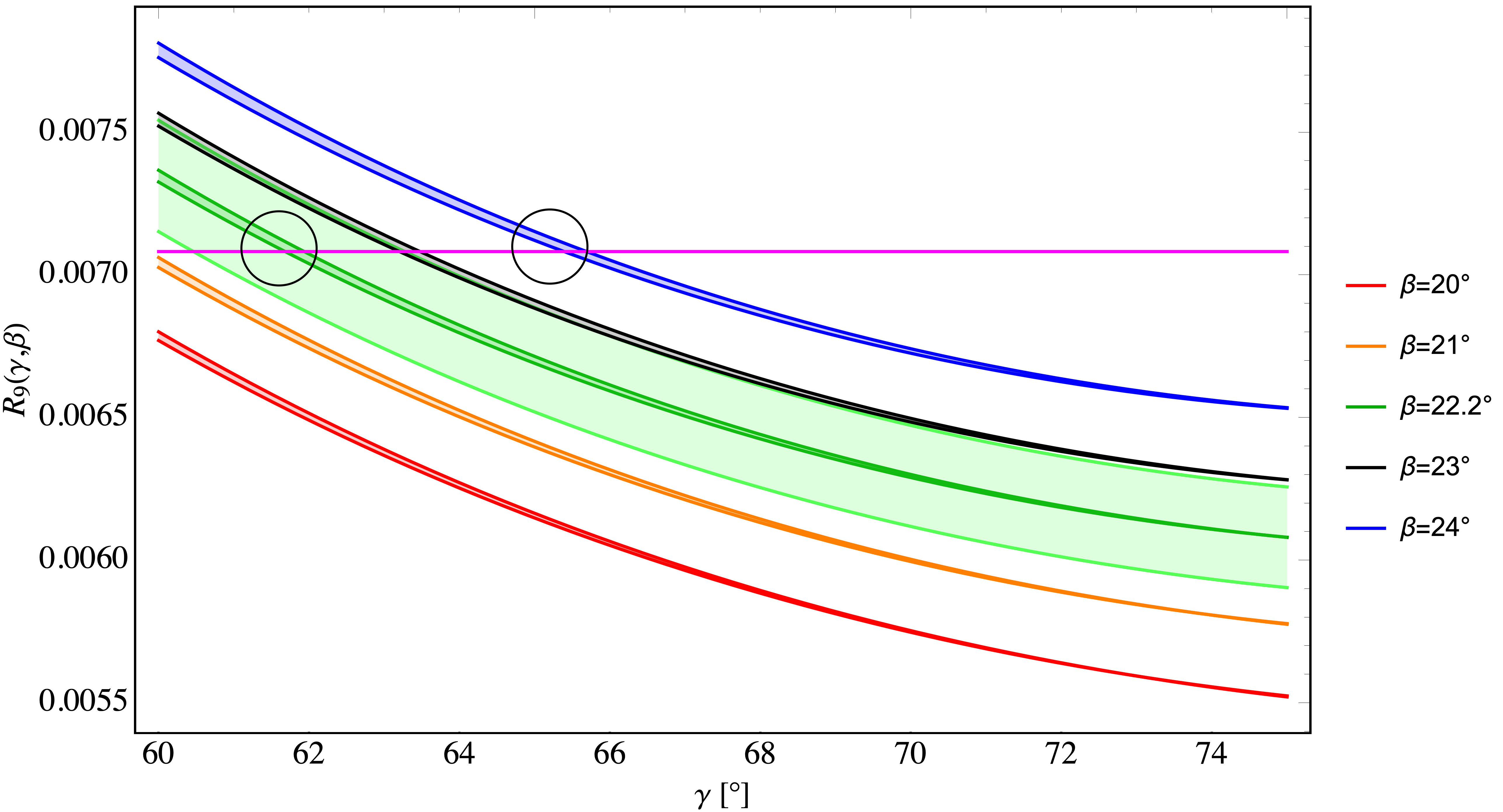
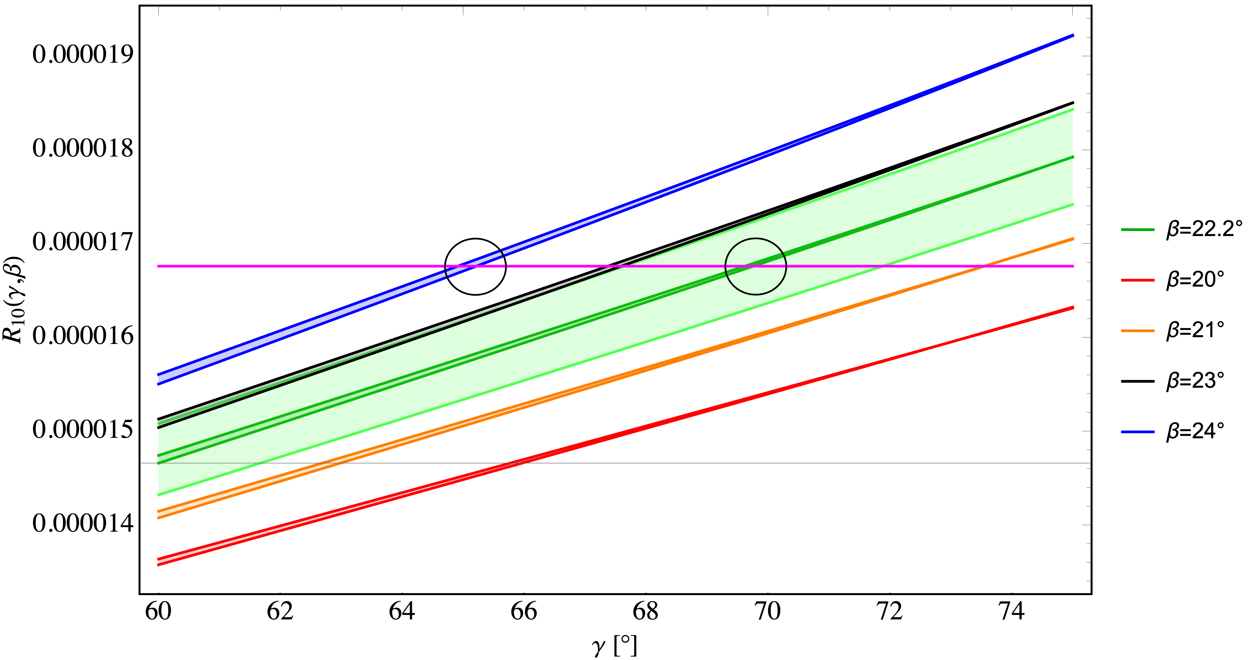
Figure 14: The ratios $R_{9}$ and $R_{10}$ as functions of $\gamma$ for different values of $\beta$. The coloured bands correspond to $38<|V_{cb}|\times 10^{3}<43$. The horizontal thin bands represent the experimental values as given in (89). The light green band corresponds to the range $21.5^{\circ}<\beta<22.9^{\circ}$, with $38\times 10^{-3}<|V_{cb}|<43\times 10^{-3}$.

While, in view of large experimental errors, it would be premature to include presently the rare decays in this analysis, we will next use the results for $|V_{cb}|$ that are extracted from $\varepsilon_{K}$, $\Delta M_{s}$ and $\Delta M_{d}$ for rare decays.

3.4 Improved SM Predictions for rare $K$ and $B$ Decays

Beginning with $K^{+}\rightarrow\pi^{+}\nu\bar{\nu}$ and $K_{L}\rightarrow\pi^{0}\nu\bar{\nu}$, the authors of [7] obtained the results in (3) by performing first a careful analysis of theoretical uncertainties in the evaluation of both branching ratios in question and subsequently using the CKM parameters listed in PDG [8] that strictly speaking come from CKMfitters with $|V_{cb}|$ in the ballpark of its exclusive determinations. If they used UTfitters result, also listed there, they would get significantly larger values for both branching ratios because in the latter analysis the value of $|V_{cb}|$ closer to its inclusive determinations has been used.

The virtue of the strategies presented in our paper is that we can avoid all such uncertainties by simply inserting the formula (67) into the formulae for $K^{+}\rightarrow\pi^{+}\nu\bar{\nu}$ and $K_{L}\rightarrow\pi^{0}\nu\bar{\nu}$ decay branching ratios and study their dependence on $\gamma$, $\beta$ and $|V_{us}|$ in a $|V_{cb}|$-independent manner. To our knowledge such a $|V_{cb}|$-independent analysis of rare $K$ decay branching ratios has not been presented in the literature. As we will now demonstrate this allows to determine both branching ratio not only independently of the value of $|V_{cb}|$ but practically also independently of the value of the angle $\gamma$. The main parametric uncertainty comes then from $\beta$ which, as seen in (5), is already known rather precisely from the measurement of $S_{\psi K_{S}}$. The theoretical uncertainties are as in [7] but the fact that the CKM uncertainties have been practically reduced to the one in $\beta$ allows to obtain results even more accurate than listed in (3) without any worries about $|V_{cb}|$ and $\gamma$. However, in addition to the experimental error on $\varepsilon_{K}$ we have to take the theoretical ones in $r_{1}$ and $r_{2}$ in (66), in particular the ones due to $\kappa_{\epsilon}$ and $\hat{B}_{K}$. But these uncertainties have only small impact on the final errors.

We proceed then as follows. From (21), (22) and (83) we find approximate formulae

$$\boxed{R_{11}=\frac{\mathcal{B}(K^{+}\rightarrow\pi^{+}\nu\bar{\nu})}{|\varepsilon_{K}|^{0.82}}=(1.31\pm 0.05)\times 10^{-8}{\left(\frac{\sin\gamma}{\sin 67^{\circ}}\right)^{0.015}\left(\frac{\sin 22.2^{\circ}}{\sin\beta}\right)^{0.71},}}$$ (90)

$$\boxed{R_{12}=\frac{\mathcal{B}(K_{L}\rightarrow\pi^{0}\nu\bar{\nu})}{|\varepsilon_{K}|^{1.18}}=(3.87\pm 0.06)\times 10^{-8}{\left(\frac{\sin\gamma}{\sin 67^{\circ}}\right)^{0.03}\left(\frac{\sin\beta}{\sin 22.2^{\circ}}\right)^{0.9{8}}}}$$ (91)

and

$$\frac{\mathcal{B}(K_{L}\rightarrow\pi^{0}\nu\bar{\nu})}{\mathcal{B}(K^{+}\rightarrow\pi^{+}\nu\bar{\nu})}={(2.95\pm 0.12)}\,|\varepsilon_{K}|^{0.36}{\left(\frac{\sin\gamma}{\sin 67^{\circ}}\right)^{0.015}\left(\frac{\sin\beta}{\sin 22.2^{\circ}}\right)^{1.6{9}}\,.}$$ (92)

The first two of these formulae express explicitly the fact that combining on the one hand $K^{+}\rightarrow\pi^{+}\nu\bar{\nu}$ and $\varepsilon_{K}$ and on the other hand $K_{L}\rightarrow\pi^{0}\nu\bar{\nu}$ and $\varepsilon_{K}$ allows within the SM to determine to a very good approximation the angle $\beta$ independently of the value of $|V_{cb}|$ and $\gamma$. The last one just follows from them. Indeed the dependence on $\gamma$ is very weak.

But these formulae are only approximate and therefore, in what follows, we use exact formulae. In Fig. 15 we present in the upper panels $K^{+}\rightarrow\pi^{+}\nu\bar{\nu}$ and $K_{L}\rightarrow\pi^{0}\nu\bar{\nu}$ branching ratios within the SM as functions of $\gamma$ for different values of $\beta$, once the $|V_{cb}|$ dependence has been eliminated through (67). The dependence on $|V_{us}|$ is very weak. In lower panels we show $K^{+}\rightarrow\pi^{+}\nu\bar{\nu}$ and $K_{L}\rightarrow\pi^{0}\nu\bar{\nu}$ branching as functions of $\beta$ for different values of $\gamma$ We make the following observations.

• The $\gamma$ dependence is extremely weak in both cases, while the $\beta$ dependence is significant. This is in accordance with (90) and (91).

• In particular, the $\gamma$ dependence of the $K^{+}\rightarrow\pi^{+}\nu\bar{\nu}$ branching ratio is practically absent when the $\varepsilon_{K}$ is used. In fact, one can notice that the $\gamma$ dependence in (90) is even weaker than in (91). This is related to the decrease of $|V_{cb}|$ with increasing $\gamma$ as seen in Fig. 12 and these two effects of respectively suppressing and enhancing the $K^{+}\rightarrow\pi^{+}\nu\bar{\nu}$ branching ratio compensate each other. With a precise value of experimental $K^{+}\rightarrow\pi^{+}\nu\bar{\nu}$ branching ratio the value of $\beta$ could be determined without any involvement of $K_{L}\rightarrow\pi^{0}\nu\bar{\nu}$.

• On the other hand the dependence on $\beta$ in the case of $K_{L}\rightarrow\pi^{0}\nu\bar{\nu}$ is stronger than for $K^{+}\rightarrow\pi^{+}\nu\bar{\nu}$, again in agreement with (90) and (91). Therefore this time $\beta$ could be determined from $K_{L}\rightarrow\pi^{0}\nu\bar{\nu}$ without any involment of $K^{+}\rightarrow\pi^{+}\nu\bar{\nu}$.

In studying these plots one should again keep in mind that on the basis of the measurement of $S_{\psi K_{S}}$ the $1\sigma$ range for $\beta$ is given in (68). We show this range as green bands in the plots in Fig. 15. Therefore in the final step we impose this constraint. Performing the error analysis we find then from $\varepsilon_{K}$ and $S_{\psi K_{S}}$ with $60^{\circ}\leq\gamma\leq 75^{\circ}$ the result in (7). To this end we have taken into account the experimental and theoretical uncertainties in $\varepsilon_{K}$, experimental ones in the $S_{\psi K_{S}}$ measurements and the non-parametric errors of the considered branching ratios like $P_{c}$ in the case of $K^{+}\rightarrow\pi^{+}\nu\bar{\nu}$. The dominant source of uncertainty in $K^{+}\rightarrow\pi^{+}\nu\bar{\nu}$ are $P_{c}$ and $\beta$, while in the case of $K_{L}\rightarrow\pi^{0}\nu\bar{\nu}$ it is $\beta$.

We observe that both branching ratios have significantly smaller errors than the ones in (2) and (3). They supersede the usual quoted values in (2).

Decay	Branching Ratio	Decay	Branching Ratio
$K^{+}\rightarrow\pi^{+}\nu\bar{\nu}$	$(8.60\pm 0.42)\times 10^{-11}$	$B_{s}\to\mu^{+}\mu^{-}$	$(3.62^{+0.15}_{-0.10})\times 10^{-9}$
$K_{L}\rightarrow\pi^{0}\nu\bar{\nu}$	$(2.94\pm 0.15)\times 10^{-11}$	$B_{d}\to\mu^{+}\mu^{-}$	$(0.99^{+0.05}_{-0.03})\ \times 10^{-10}$
$K_{S}\to\mu^{+}\mu^{-}$	$(1.85\pm 0.10)\times 10^{-13}$	$B^{+}\to K^{+}\nu\bar{\nu}$	$(4.45\pm 0.62)\times 10^{-6}$
		$B^{0}\to K^{0*}\nu\bar{\nu}$	$(9.70\pm 0.92)\times 10^{-6}$

Table 2: Present most accurate $|V_{cb}|$-independent SM estimates of the branching ratios considered in the paper. The $\gamma$ dependence is either very small or absent. See the text for details.

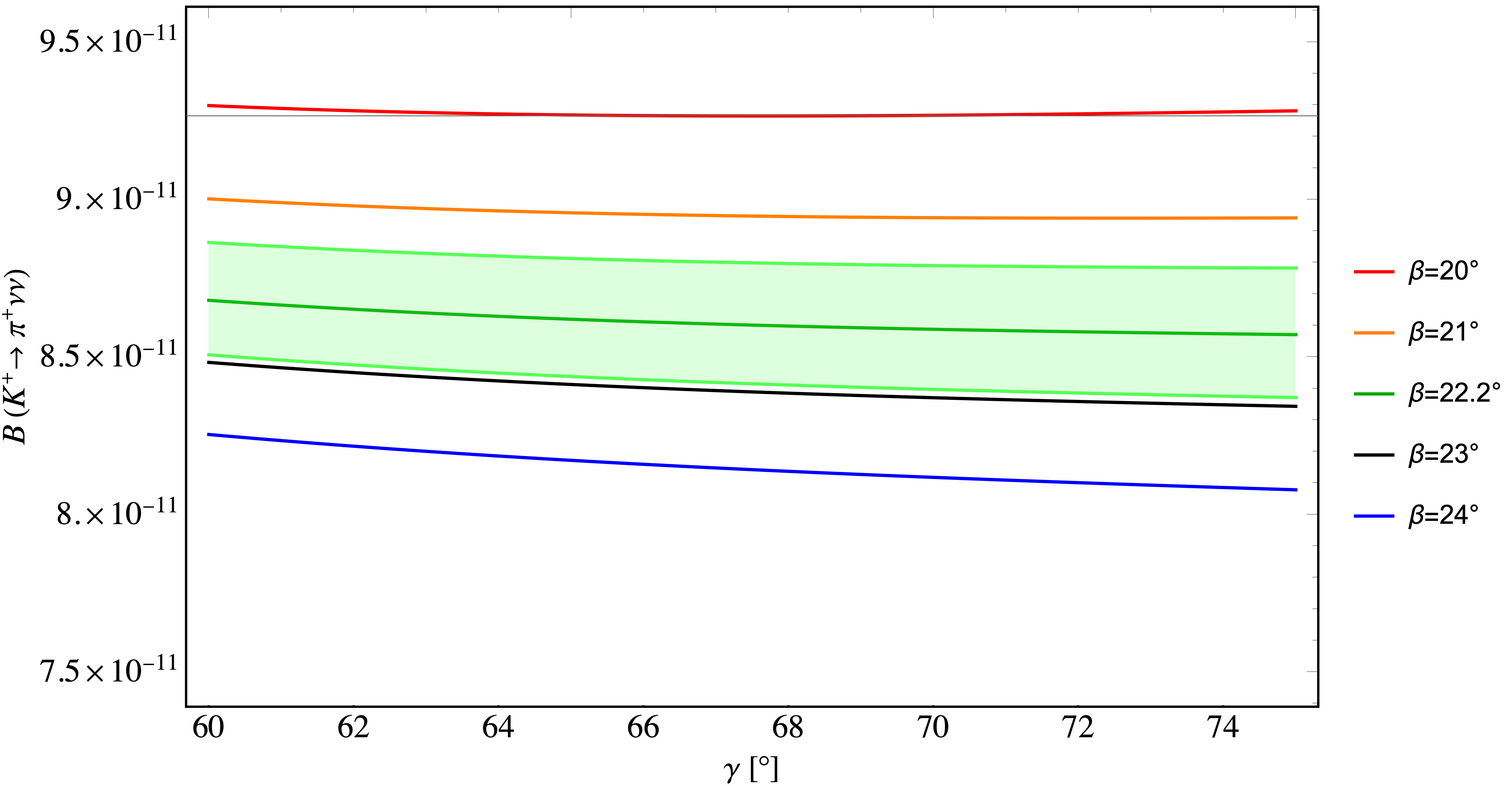
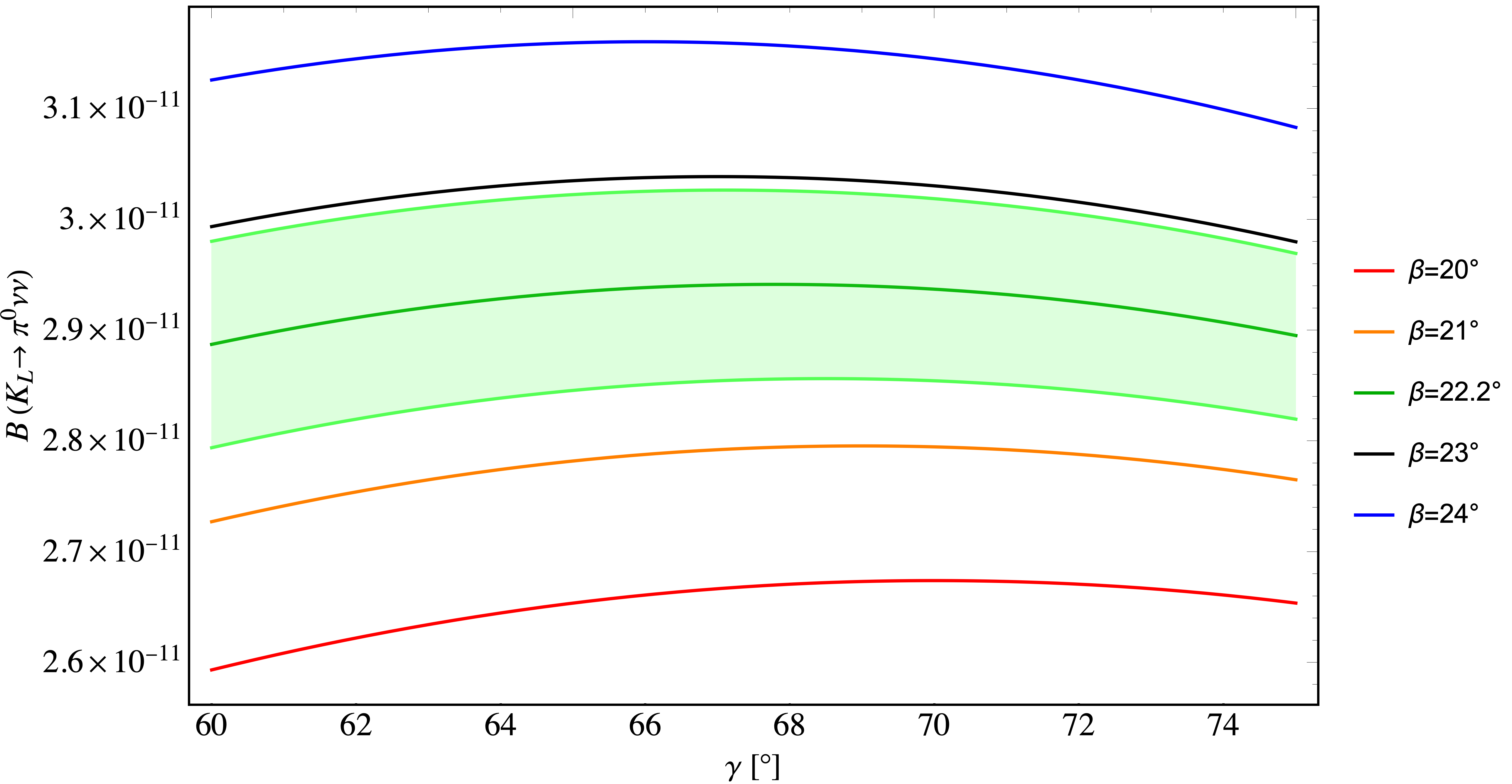
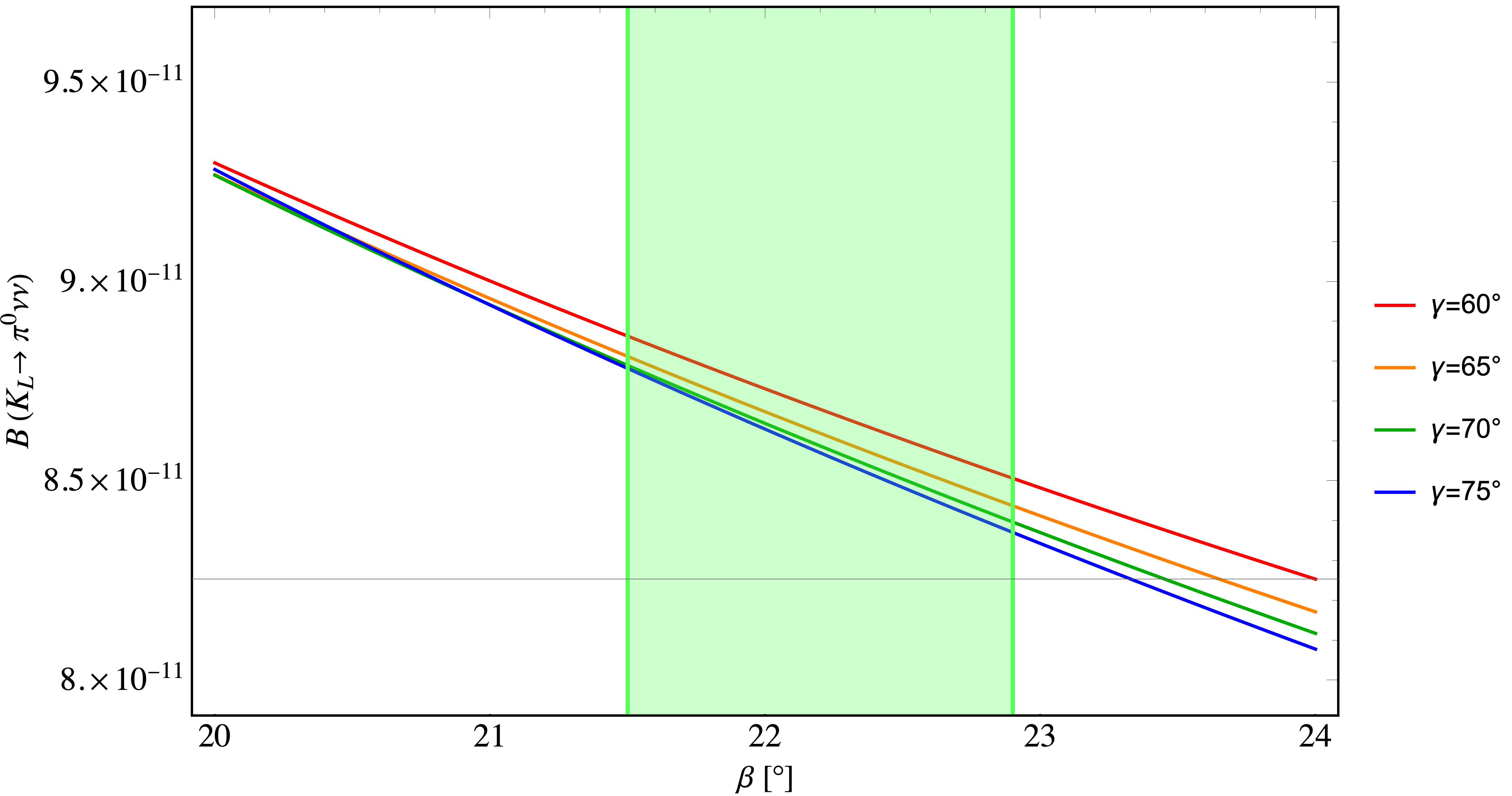
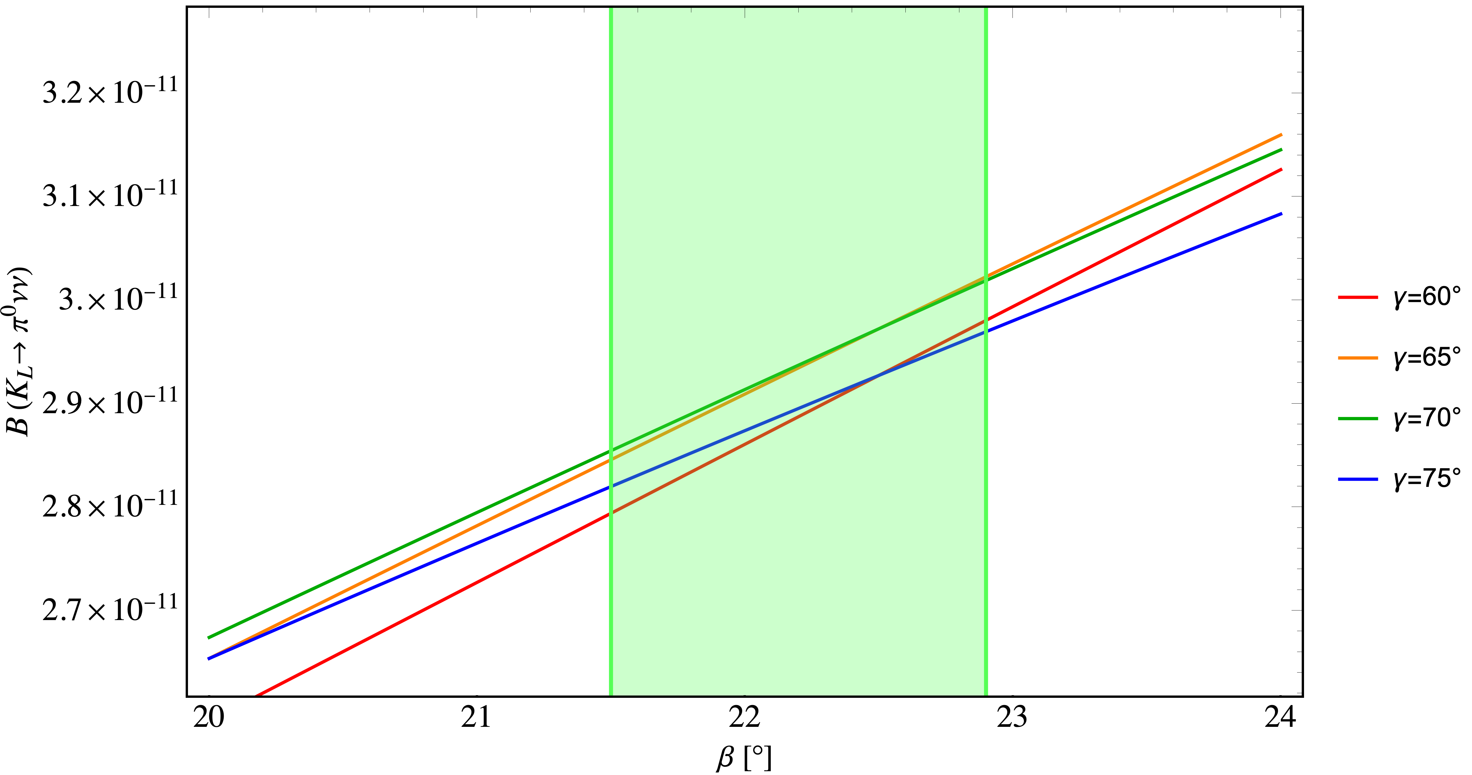
Figure 15: The dependence of the branching ratios $\mathcal{B}(K^{+}\rightarrow\pi^{+}\nu\bar{\nu})$ (left panels) and $\mathcal{B}(K_{L}\rightarrow\pi^{0}\nu\bar{\nu})$ (right panels) on $\gamma$ for different values of $\beta=20.0^{\circ},21.0^{\circ},22.0^{\circ},23.0^{\circ},24.0^{\circ}$ and on $\beta$ for different values of $\gamma=60.0^{\circ},65.0^{\circ},70.0^{\circ},75^{\circ}$. $\varepsilon_{K}$ has been fixed to its experimental value.

For $B_{s,d}\to\mu^{+}\mu^{-}$ decays analogous use of $\Delta M_{s,d}$ eliminates the CKM dependence from branching ratios as already demonstrated in [32, 33] with the result given in (8). Inserting next the results in (7) and (8) into the $|V_{cb}|$-independent ratios $R_{7}$, $R_{8}$ and $R_{\rm SL}$ allows in turn to obtain the most precise estimate of the branching ratios of $K_{S}\to\mu^{+}\mu^{-}$, $B^{+}\to K^{+}\nu\bar{\nu}$ and $B^{0}\to K^{0*}\nu\bar{\nu}$ as well. The results for all branching ratios are summarized in Table 2 and their implications in the case of $K^{+}\rightarrow\pi^{+}\nu\bar{\nu}$ and $B_{s}\to\mu^{+}\mu^{-}$ in Fig. 7.

It should be emphasized that to obtain precise SM predictions like the ones in (7) and (8) it is crucial to choose the proper pairs of observables. For instance combining $K^{+}\rightarrow\pi^{+}\nu\bar{\nu}$ with $\Delta M_{s}$ or $B_{s}\to\mu^{+}\mu^{-}$ with $\varepsilon_{K}$ would not allow us precise predictions for $K^{+}\rightarrow\pi^{+}\nu\bar{\nu}$ and $B_{s}\to\mu^{+}\mu^{-}$ even after the elimination of the $|V_{cb}|$ because of the left-over $\gamma$ dependence in both cases. Moreover selecting a subset of optimal observables for a given SM prediction avoids the assumption of the absence of NP in other observables which would be questionable in view of the inconsistencies between various determinations of $|V_{cb}|$ identified by us.

The accuracy of our predictions could certainly be improved through a better determination of $\beta$ with the help of $S_{\psi K_{s}}$ or a better determination of $|V_{ub}|$. As an example we refer to a recent determination of $|V_{ub}|$ with the help of exclusive semi-leptonic $B$ decays with $|V_{ub}|=3.68(5)\times 10^{-3}$ [97], that is more accurate than what we obtained in (82). Through (13) using this result a more accurate $\beta=22.4(5)^{\circ}$ can be determined. Adding this additional constraint we find

$${\mathcal{B}(K^{+}\rightarrow\pi^{+}\nu\bar{\nu})_{\text{SM}}={(8.55\pm 0.37)}\times 10^{-11}\,,\quad\mathcal{B}(K_{L}\rightarrow\pi^{0}\nu\bar{\nu})_{\text{SM}}={(2.97\pm 0.12)}\times 10^{-11}\,,}$$ (93)

that is slightly more accurate than our results in (7). However, we keep (7) as our official result until the impressive determination of $|V_{ub}|$ in [97] will be confirmed by other experts on exclusive semi-leptonic $B$ decays.

4 A Guide to $|V_{cb}|$-independent Relations

In the course of our analysis we have introduced various ratios and relations between different observables of which some were independent of $|V_{cb}|$ and the rest practically independent of it, that is with the dependence on $|V_{cb}|$ significantly below $1\%$ in the full range of $|V_{cb}|$ considered by us. We have also checked that the dependence on $|V_{us}|=\lambda$ of these relations and ratios was either absent or totally negligible. Consequently the only relevant dependences which were left were only on the angles $\beta$ and $\gamma$.

The basis for the derivation of these correlations were approximate but accurate formulae with the general power-like structure

$${\mathcal{B}(\text{Decay}_{i})=C_{i}|V_{cb}|^{r_{1}}[\sin\gamma]^{r_{2}}[\sin\beta]^{r_{3}},}$$ (94)

with the coefficients $C_{i}$ either being constants or being very weakly dependent on $\beta$ and $\gamma$ like the function $G(\beta,\gamma)$. The powers $r_{i}$ can be regarded as critical exponents of flavour physics. In Table 3 we collect these critical exponents for all observables considered by us and give references to the corresponding expressions with the power-like structure. Expressing then $|V_{cb}|$ in terms of a given branching ratio and inserting it into a power-like formula for another branching ratio allows to derive analytically all correlations presented in our paper. One finds then that some of the ratios are independent of $\beta$ and $\gamma$, some are dependent only on $\gamma$, some only on $\beta$ and some on both $\beta$ and $\gamma$.

Observable	$r_{1}$	$r_{2}$	$r_{3}$	Formula
$K^{+}\rightarrow\pi^{+}\nu\bar{\nu}$,	$2.8$	$1.39$	$0.0$	(21)
$K_{L}\rightarrow\pi^{0}\nu\bar{\nu}$,	$4.0$	$2.0$	$2.0$	(22)
$K_{S}\to\mu^{+}\mu^{-}$,	$4.0$	$2.0$	$2.0$	(30)
$|\varepsilon_{K}|$,	$3.4$	$1.67$	$0.87$	(83)
$B_{s}\to\mu^{+}\mu^{-}$	$4.0$	$0.0$	$0.0$	(34)
$B_{d}\to\mu^{+}\mu^{-}$	$2.0$	$2.0$	$0.0$	(36)
$B^{+}\to K^{+}\nu\bar{\nu}$	$2.0$	$0.0$	$0.0$	(52)
$B^{0}\to K^{0*}\nu\bar{\nu}$	$2.0$	$0.0$	$0.0$	(53)
$\Delta M_{d}$	$2.0$	$2.0$	$0.0$	(69)
$\Delta M_{s}$	$2.0$	$0.0$	$0.0$	(70)

Table 3: Critical exponents of flavour physics entering the formula (94). In the last column the reference to the given power-like formula is given.

In Table 4 we indicate which of the relations found by us has weak, strong or none dependence on $\beta$ and $\gamma$, where ”none” stands also for a dependence that induces a ratio variation of less than $0.5\%$, in the considered ranges. This table allows to find in no time the analytic expressions for each relation in the text and the corresponding plot as a function of $\gamma$ for different values of $\beta$. The ratios $R_{q}$ proposed in [32] and analyzed recently in [33] are defined through

$$R_{q}=\frac{\mathcal{B}(B_{q}\to\mu^{+}\mu^{-})}{\Delta M_{q}}=C\frac{\tau_{B_{q}}}{\hat{B}_{q}}\frac{(Y_{0}(x_{t}))^{2}}{S_{0}(x_{t})},\qquad q=d,s\,,$$ (95)

with

$$C=6\pi\frac{1}{\eta_{B}^{2}}\left(\frac{\alpha}{4\pi\sin^{2}\theta_{W}}\right)^{2}\frac{m_{\mu}^{2}}{M_{W}^{2}}=4.291\times 10^{-10}\,.$$ (96)

They are CKM independent and have been used to obtain the results in (8).

We would like to emphasize that among sixteen ratios listed in Table 4 only $R_{7}$, $R_{9}$, $R_{10}$ and $R_{s}$ could be confronted until now with the data. As $R_{9}$ and $R_{10}$ depend strongly on $\gamma$ no definite conclusion on them could be reached but as we discussed in the previous section and seen in Fig. 14 it is not possible to obtain simultaneous agreement on both with very precise data for any value of $\gamma$ if the constraint from $S_{\psi K_{S}}$ is taken into account. On the other hand $R_{7}$ and $R_{s}$ are independent of CKM parameters and it was interesting to find that in both cases some tensions with the data have been identified. It will be interesting to compare one day all sixteen ratios with future data. In particular when the value of $\gamma$ will be known with high precision we will be able to check if all these ratios agree with the improved data. If this will not be the case the pattern of possible deviations from the SM predictions calculated by us may give some hints for the particular NP at work. Therefore we are looking forward to the day on which the angle $\gamma$ will be precisely known and all branching ratios analysed by us accurately measured. Then we will be able to replace the last two columns in Table 4 by SM predictions for these ratios and the corresponding data.

Ratio	Observables	$\beta$	$\gamma$	Formula	Figure
$R_{0}$	$K^{+}\rightarrow\pi^{+}\nu\bar{\nu}$, $K_{L}\rightarrow\pi^{0}\nu\bar{\nu}$	strong	none	(25)	4
$R_{1}$	$K^{+}\rightarrow\pi^{+}\nu\bar{\nu}$, $B_{s}\to\mu^{+}\mu^{-}$	none	strong	(41)	6
$R_{2}$	$K^{+}\rightarrow\pi^{+}\nu\bar{\nu}$, $B_{d}\to\mu^{+}\mu^{-}$	none	strong	(44)	6
$R_{3}$	$K_{L}\rightarrow\pi^{0}\nu\bar{\nu}$, $B_{s}\to\mu^{+}\mu^{-}$	strong	strong	(50)	9
$R_{4}$	$K_{L}\rightarrow\pi^{0}\nu\bar{\nu}$, $B_{d}\to\mu^{+}\mu^{-}$	strong	strong	(51)	9
$R_{5}$	$K^{+}\rightarrow\pi^{+}\nu\bar{\nu}$, $B^{+}\to K^{+}\nu\bar{\nu}$	none	strong	(55)	10
$R_{6}$	$K^{+}\rightarrow\pi^{+}\nu\bar{\nu}$, $B^{0}\to K^{0*}\nu\bar{\nu}$	none	strong	(56)	10
$R_{7}$	$B_{s}\to\mu^{+}\mu^{-}$, $B^{+}\to K^{+}\nu\bar{\nu}$	none	none	(58)	$-$
$R_{8}$	$B_{s}\to\mu^{+}\mu^{-}$, $B^{0}\to K^{0*}\nu\bar{\nu}$	none	none	(59)	$-$
$R_{9}$	$|\varepsilon_{K}|$, $\Delta M_{d}$	strong	strong	(85)	14
$R_{10}$	$|\varepsilon_{K}|$, $\Delta M_{s}$	strong	strong	(86)	14
$R_{11}$	$K^{+}\rightarrow\pi^{+}\nu\bar{\nu}$, $|\varepsilon_{K}|$	strong	none	(90)	15
$R_{12}$	$K_{L}\rightarrow\pi^{0}\nu\bar{\nu}$, $|\varepsilon_{K}|$,	strong	none	(91)	15
$R_{d}$	$B_{d}\to\mu^{+}\mu^{-}$, $\Delta M_{d}$	none	none	(95)	$-$
$R_{s}$	$B_{s}\to\mu^{+}\mu^{-}$, $\Delta M_{s}$	none	none	(95)	$-$
$R_{\rm SL}$	$K_{L}\rightarrow\pi^{0}\nu\bar{\nu}$, $K_{S}\to\mu^{+}\mu^{-}$	none	none	(33)	$-$

Table 4: Guide to the relations presented in the paper. We distinguish between strong, weak and none dependences on $\beta$ and $\gamma$. In the last two columns the reference to the formula for a given ratio and to the corresponding plot are given.

5 Conclusions

In the present paper, following and extending significantly the strategies of [34, 35, 36, 29, 5, 32, 33, 28], we have proposed to search for NP in rare Kaon and $B$-meson decays without the necessity to choose the values of the CKM elements $|V_{cb}|$ and $|V_{ub}|$, that introduce presently large parametric uncertainties in the otherwise theoretically clean decays $K^{+}\rightarrow\pi^{+}\nu\bar{\nu}$, $K_{L}\rightarrow\pi^{0}\nu\bar{\nu}$, $K_{S}\to\mu^{+}\mu^{-}$, $B_{s,d}\to\mu^{+}\mu^{-}$, $B\to K(K^{*})\nu\bar{\nu}$, in the parameter $\varepsilon_{K}$ and $\Delta M_{s,d}$. Table 4 is a useful guide to $|V_{cb}|$-independent relations and corresponding figures obtained in our paper.

In addition to various updates and to stressing the usefulness of the set (4) [29, 28] the main results of our present paper are as follows.

• We reemphasized that despite the strong dependence of the branching ratios for $K^{+}\rightarrow\pi^{+}\nu\bar{\nu}$ and $K_{L}\rightarrow\pi^{0}\nu\bar{\nu}$ on $|V_{cb}|$ the correlation between them within the SM and models with CMFV, as given analytically in (25) and numerically in Fig. 4, is practically independent of $|V_{cb}|$ and $\gamma$ [34]. The dependence of this correlation on $\beta$ can be in principle used for the extraction of $\beta$ [34].

• We discussed the correlation between the branching ratios for $K^{+}\rightarrow\pi^{+}\nu\bar{\nu}$ and $B_{s}\to\mu^{+}\mu^{-}$ in (41), already proposed in [5], but here presented in a different manner. In particular we introduced the ratios $R_{1}$ and $R_{2}$, in (45), of the branching ratio for $K^{+}\rightarrow\pi^{+}\nu\bar{\nu}$ to the branching ratios for $B_{s}\to\mu^{+}\mu^{-}$ and $B_{d}\to\mu^{+}\mu^{-}$ raised both to the power of $1.4$. While, as seen in Figs. 2 and 5, all these branching ratios depend strongly on $|V_{cb}|$, $R_{1}$ and $R_{2}$ are to an excellent approximation $|V_{cb}|$-independent. They exhibit then only a sizable dependence on $\gamma$ and a very weak one on $\beta$ as seen in Fig. 6. Even more interesting will be the plots in Fig. 7 when the precision on both branching ratios and $\gamma$ will be increased in the coming years.

• We presented an improved, relative to [5], triple correlation between the branching ratios for $K^{+}\rightarrow\pi^{+}\nu\bar{\nu}$, $B_{s}\to\mu^{+}\mu^{-}$ and $B_{d}\to\mu^{+}\mu^{-}$ in (47) that practically does not depend on the CKM parameters within the SM .

• We discussed the correlations between the branching ratios for $K^{+}\rightarrow\pi^{+}\nu\bar{\nu}$ and $K_{L}\rightarrow\pi^{0}\nu\bar{\nu}$ with the branching ratios for $B_{s,d}\to\mu^{+}\mu^{-}$ and $B\to K(K^{*})\nu\bar{\nu}$ represented by the $|V_{cb}|$-independent ratios $R_{3}-R_{6}$ in (49) and (54). The $\gamma$ and $\beta$ dependence of $R_{3}$ and $R_{4}$ has been shown in Fig. 9 and the one of $R_{5}$ and $R_{6}$ in Fig. 10.

• On the other hand the ratios of $B\to K(K^{*})\nu\bar{\nu}$ branching ratios to the $B_{s}\to\mu^{+}\mu^{-}$ one as well as the ratio of the short distance contribution to the $K_{S}\to\mu^{+}\mu^{-}$ branching ratio and the one for $K_{L}\rightarrow\pi^{0}\nu\bar{\nu}$ in the SM are independent of CKM parameters except for $\lambda$. These correlations can be found in (58), (59) and in (33). In this context we have pointed out that the ratio of the branching ratios for $B^{+}\to K^{+}\nu\bar{\nu}$ and $B_{s}\to\mu^{+}\mu^{-}$ from Belle II and LHCb signals a $1.8\sigma$ tension with its SM value.

• In the context of the determination of $\gamma$ by means of the ratio $\Delta M_{d}/\Delta M_{s}$ we have emphasized that the tension between this determination and the one from tree-level $B$-decays pointed out in 2016 in [37] diminished. The final verdict will be given by future precise measurements of $\gamma$ by the LHCb and Belle II collaborations [98, 99] that could reach the precision of $\pm 1^{\circ}$.

• We have proposed a test of the SM that is complementary to the usual UT-analyses. It exhibits the parameter $|V_{cb}|$ hidden in the latter analyses. To this end we proposed to extract from a given observable the value of $|V_{cb}|$ as a function of $\beta$ and $\gamma$ for which the SM agrees with the experimental data. We have illustrated this idea considering $\varepsilon_{K}$, $\Delta M_{s}$ and $\Delta M_{d}$ for which both theory and experiment reached already good precision. The result is presented in Fig. 12. We find that, when $\varepsilon_{K}$ and $\Delta M_{d}$ are considered simultaneously and the data on $S_{\psi K_{S}}$ are taken into account, $\gamma=61.3(1.6)^{\circ}$ and $|V_{cb}|=43.1(1.0)\times 10^{-3}$ are obtained. But when $\varepsilon_{K}$ and $\Delta M_{s}$ are simultaneously considered we find $\gamma=70.3(2.6)^{\circ}$ and $|V_{cb}|=41.7(6)\times 10^{-3}$. In order to exhibit this tension in a $|V_{cb}|$-independent manner we considered suitable ratios of $\varepsilon_{K}$ and $\Delta M_{d,s}$ that do not depend on $|V_{cb}|$. The result is presented in Fig. 14. As seen in Figs. 12 and 14 the agreement between these two determinations can only be obtained for a value of $\beta$ that differs by $2\sigma$ from the one obtained from $S_{\psi K_{S}}$.

• We conclude therefore that it is not possible to obtain full agreement between the data on $\varepsilon_{K}$, $\Delta M_{d}$, $\Delta M_{s}$ and $S_{\psi K_{S}}$ within the SM independently of the value of $|V_{cb}|$ and $\gamma$. While this tension is still moderate it hints for some NP at work. In this context a precise measurement of $\gamma$ will be important. If its value will turn out to be in the ballpark of $66^{\circ}$ as signalled by the most recent LHCb result, a new CP-violating phase will be required to obtain the agreement with the data on $S_{\psi K_{S}}$.

• In the context of these investigations we have pointed out that $\Delta M_{s}$ offers presently the best estimate of $|V_{cb}|$ in the SM if only one quantity is considered. The result is shown in Fig. 12 and given in (75) and in (76), where in the latter also the $\epsilon_{K}$ and $S_{\psi K_{S}}$ measurements are taken into account. Including $S_{\psi K_{S}}$ allows to determine $|V_{ub}|$ as well so that in summary we find

  $$\boxed{|V_{cb}|=41.8(6)\times 10^{-3},\qquad|V_{ub}|=3.65(12)\times 10^{-3}.}$$ (97)

  This value of $|V_{ub}|$ is in perfect agreement with the FLAG’s value in (81) while the one for $|V_{cb}|$ agrees well with the UTfit determination $|V_{cb}|=42.0(6)\times 10^{-3}$. On the other hand it is significantly higher than the CKMfit one, i.e. $|V_{cb}|=40.5(8)\times 10^{-3}$.

• We obtained the analytical expression for $|V_{cb}|$ corresponding to the experimental value of $\varepsilon_{K}$, that is a function of $\gamma$ and $\beta$. Having eliminated the $|V_{cb}|$ dependence this allowed to study transparently the $\gamma$ and $\beta$ dependences of $K^{+}\rightarrow\pi^{+}\nu\bar{\nu}$ and $K_{L}\rightarrow\pi^{0}\nu\bar{\nu}$ branching ratios. The results for $K^{+}\rightarrow\pi^{+}\nu\bar{\nu}$ and $K_{L}\rightarrow\pi^{0}\nu\bar{\nu}$ are presented in Fig. 15. For $B_{s,d}$ decays it is more convenient to use $\Delta M_{s,d}$ for this purpose as this eliminates the CKM dependence from branching ratios as already demonstrated in [32, 33].

However, at present the most important results of our paper appear to be precise predictions for $K\to\pi\nu\bar{\nu}$ branching ratios in (7) and for $B_{s,d}\to\mu^{+}\mu^{-}$ in (8) that supersede the results quoted in the literature. Beyond the $|V_{cb}|$-independence their virtues are as follows.

• In the case of $K^{+}\rightarrow\pi^{+}\nu\bar{\nu}$ and $K_{L}\rightarrow\pi^{0}\nu\bar{\nu}$ the $\gamma$ dependence is very weak as seen in (90) and (91) and the only relevant CKM dependence comes from the angle $\beta$ that is already accurately determined by $S_{\psi K_{S}}$. Both uncertainties in $\beta$ and $\gamma$ have been included in the errors. In particular the one from $\gamma$ corresponds to the range $60^{\circ}\leq\gamma\leq 75^{\circ}$ that is significantly larger than the one resulting from global CKM fits.

• In the case of $B_{s,d}\to\mu^{+}\mu^{-}$, as seen in (95) no CKM dependence is involved so that the result is independent of any CKM global fits.

Having these results allowed us to obtain the best estimate of the branching ratios of $K_{S}\to\mu^{+}\mu^{-}$, $B^{+}\to K^{+}\nu\bar{\nu}$ and $B^{0}\to K^{0*}\nu\bar{\nu}$ as well. The results for all branching ratios are summarized in Table 2 and their implications in the case of $K^{+}\rightarrow\pi^{+}\nu\bar{\nu}$ and $B_{s}\to\mu^{+}\mu^{-}$ in Fig. 7.

The future of our strategies will depend on the precision on the determination of $\gamma$ and $\beta$ in those tree-level decays in which it can be demonstrated that NP contributes in a negligible way. In this context LHCb and Belle II experiments aiming at $1^{\circ}$ accuracy for $\gamma$ could contribute in an important manner.

However, similar to what was stated in [33], we also emphasize that taking ratios of observables cancels not only parametric, theoretical and experimental uncertainties. It can in principle cancel also some NP effects that could be present, in our case, in $K^{+}\rightarrow\pi^{+}\nu\bar{\nu}$, $K_{L}\rightarrow\pi^{0}\nu\bar{\nu}$, $K_{S}\to\mu^{+}\mu^{-}$, $B_{s,d}\to\mu^{+}\mu^{-}$, $B\to K(K^{*})\nu\bar{\nu}$, $|\varepsilon_{K}|$ and in the ratio of the mass differences $\Delta M_{s,d}$. Therefore the complete search for NP must also consider eventually all observables separately that brings back CKM uncertainties and in certain cases also hadronic uncertainties. Yet, the strategies presented here allow to test the mutual consistency of various correlations predicted by the SM without the worry about the values of $|V_{cb}|$ and $|V_{ub}|$. This simplifies the search for NP through the violation of these SM correlations. Indeed, it was already possible to conclude in [33] that some NP is hinted in the SM correlation between $\overline{\mathcal{B}}(B_{s}\to\mu^{+}\mu^{-})$ and $\Delta M_{s}$. Similar tension seems to be hinted in the correlation between $\overline{\mathcal{B}}(B_{s}\to\mu^{+}\mu^{-})$ and $B^{+}\to K^{+}\nu\bar{\nu}$ pointed out here.

In this context we would like to refer to a series of papers by Fleischer and collaborators [100, 101, 102] in which, in the spirit of the proposal in [32], ratios of processes governed by the transition $b\to ul\bar{\nu}_{l}$ have been considered in order to cancel $|V_{ub}|$ dependence. Already these ratios, when compared with their SM values can, as in [33] and in the present paper, signal the presence of NP at work. Considering then these ratios in the context of different NP scenarios that can be distinguished through different operators like vector, scalar, pseudoscalar and tensor ones, the authors of [100, 101, 102] extracted from the present data the regions for the Wilson coefficients of these operators independently of the value of $|V_{ub}|$. Subsequently, using these coefficients they determined the values of $|V_{ub}|$ for each NP scenario. While this strategy is interesting in itself, it shows that at the end the value of $|V_{ub}|$ extracted from the data will depend on NP involved and taking the ratios of various observables will not avoid it. Even in specific NP scenarios considered in [100, 101, 102] it was crucial to assume that NP did not affect the coefficient of the SM left-handed operator. Without this assumption one could always rescale all Wilson coefficients by an arbitrary number which would cancel in the ratio. In turn Wilson coefficients of NP operators would not be determined and this would also be the case of $|V_{ub}|$. Imposing no NP contribution to the SM operator does not allow such rescaling and the strategy for $|V_{ub}|$ determination in the presence of NP proposed in these papers could be executed. Whether this interesting strategy is more powerful than the global fits remains to be seen when the data improves. But in any case it provides an additional insight in a possible NP at work.

In the context of the present paper we are looking forward to improved results for $K^{+}\rightarrow\pi^{+}\nu\bar{\nu}$, $K_{L}\rightarrow\pi^{0}\nu\bar{\nu}$, $K_{S}\to\mu^{+}\mu^{-}$, $B_{s,d}\to\mu^{+}\mu^{-}$, $B\to K(K^{*})\nu\bar{\nu}$ and also $\gamma$ which would allow to test several of the $|V_{cb}|$-independent correlations found by us.

Acknowledgements

We would like to thank Pietro Baratella, Jean-Marc Gérard and Peter Stangl for discussions and comments on the manuscript. A.J.B acknowledges financial support from the Excellence Cluster ORIGINS, funded by the Deutsche Forschungsgemeinschaft (DFG, German Research Foundation), Excellence Strategy, EXC-2094, 390783311. E.V. has been partially funded by the Deutsche Forschungs-gemeinschaft (DFG, German Research Foundation) under Germany’s Excellence Strategy- EXC-2094 - 390783311, by the Collaborative Research Center SFB1258 and the BMBFgrant 05H18WOCA1 and thanks the Munich Institute for Astro- and Particle Physics(MIAPP) for hospitality.

Appendix A Basic Functions

The basic functions that enter various formulae are given as follows.

For rare decays without the inclusion of QCD corrections one has

$$X_{0}(x_{t})={\frac{x_{t}}{8}}\;\left[{\frac{x_{t}+2}{x_{t}-1}}+{\frac{3x_{t}-6}{(x_{t}-1)^{2}}}\;\ln x_{t}\right]\,,$$ (98)

$$Y_{0}(x_{t})={\frac{x_{t}}{8}}\;\left[{\frac{x_{t}-4}{x_{t}-1}}+{\frac{3x_{t}}{(x_{t}-1)^{2}}}\ln x_{t}\right]\,,$$ (99)

where $x_{t}=m^{2}_{t}/M_{W}^{2}$.

The inclusion of NLO QCD corrections [15, 14] and NLO electroweak corrections [20],in the case of $X_{0}(x_{t})$ gives with the most recent value of $m_{t}(m_{t})$ in Table 1 [7]

$$X(x_{t})=1.462\pm 0.017_{\rm QCD}\pm 0.002_{\rm EW}=1.462\pm 0.017\,$$ (100)

which updates the value $X(x_{t})=1.481\pm 0.009$ used in [5] that is also quoted in [2].

The inclusion of NLO and NNLO QCD corrections and NLO electroweak correction in the case of $Y_{0}(x_{t})$ results in [41]

$$Y(x_{t})=\eta_{\text{eff}}\,Y_{0}(x_{t})\,,\qquad\eta_{\text{eff}}=0.9882\pm 0.0024\,.$$ (101)

For $\Delta M_{s,d}$ and $\varepsilon_{K}$ the relevant functions without QCD corrections are

$$S_{0}(x_{t}) = \frac{4x_{t}-11x^{2}_{t}+x^{3}_{t}}{4(1-x_{t})^{2}}-\frac{3x^{3}_{t}\ln x_{t}}{2(1-x_{t})^{3}},$$ (102)

$$S_{0}(x_{c}) = x_{c},$$ (103)

$$S_{0}(x_{c},x_{t}) = x_{c}\left[\ln\frac{x_{t}}{x_{c}}-\frac{3x_{t}}{4(1-x_{t})}-\frac{3x^{2}_{t}\ln x_{t}}{4(1-x_{t})^{2}}\right].$$ (104)

In the last two expressions we have kept only linear terms in $x_{c}\ll 1$, but of course all orders in $x_{t}$. The last function generalizes $S_{0}(x_{t})$ in (102) to include box diagrams with simultaneous top-quark and charm-quark exchanges. QCD corrections are included in the main text with the help of $\eta_{ij}$ and $\eta_{B}$ factors.

For numerical calculations one should of course use the exact expressions given above but to get an idea on the size of these functions and for derivation of analytical formulae one can use the following approximate but simple expressions

$$~{}X_{0}(x_{t})=0.660~{}x_{t}^{0.575},\qquad Y_{0}(x_{t})=0.315~{}x_{t}^{0.78},\qquad S_{0}(x_{t})=0.784~{}x_{t}^{0.76}\,.$$ (105)

In the range $160\,\text{GeV}\leq m_{t}(m_{t})\leq 165\,\text{GeV}$ these approximations reproduce the exact expressions to an accuracy better than $0.2\%$ which is sufficient for deriving analytic formulae. Then

$$X_{0}(x_{t})=1.49~{}\left(\frac{m_{t}(m_{t})}{163\,\text{GeV}}\right)^{1.15},\quad\quad Y_{0}(x_{t})=0.95~{}\left(\frac{m_{t}(m_{t})}{163\,\text{GeV}}\right)^{1.56},$$ (106)

$$S_{0}(x_{t})=2.31~{}\left(\frac{m_{t}(m_{t})}{163\,\text{GeV}}\right)^{1.52}\,.$$ (107)

References

- [1] A. J. Buras, F. Schwab, and S. Uhlig, Waiting for precise measurements of and , Rev. Mod. Phys. 80 (2008) 965–1007, [hep-ph/0405132].
- [2] A. J. Buras, Gauge Theory of Weak Decays. Cambridge University Press, 6, 2020.
- [3] NA62 Collaboration, E. Cortina Gil et al., Measurement of the very rare K+→ decay, JHEP 06 (2021) 093, [arXiv:2103.15389].
- [4] KOTO Collaboration, J. Ahn et al., Search for the and decays at the J-PARC KOTO experiment, Phys. Rev. Lett. 122 (2019), no. 2 021802, [arXiv:1810.09655].
- [5] A. J. Buras, D. Buttazzo, J. Girrbach-Noe, and R. Knegjens, and in the Standard Model: status and perspectives, JHEP 11 (2015) 033, [arXiv:1503.02693].
- [6] C. Bobeth, A. J. Buras, A. Celis, and M. Jung, Patterns of Flavour Violation in Models with Vector-Like Quarks, JHEP 04 (2017) 079, [arXiv:1609.04783].
- [7] J. Brod, M. Gorbahn, and E. Stamou, Updated Standard Model Prediction for and , in 19th International Conference on B-Physics at Frontier Machines, 5, 2021. arXiv:2105.02868.
- [8] Particle Data Group Collaboration, P. A. Zyla et al., Review of Particle Physics, PTEP 2020 (2020), no. 8 083C01.
- [9] M. Bordone, N. Gubernari, D. van Dyk, and M. Jung, Heavy-Quark expansion for form factors and unitarity bounds beyond the limit, Eur. Phys. J. C 80 (2020), no. 4 347, [arXiv:1912.09335].
- [10] M. Bordone, B. Capdevila, and P. Gambino, Three loop calculations and inclusive Vcb, Phys. Lett. B 822 (2021) 136679, [arXiv:2107.00604].
- [11] Y. Aoki et al., FLAG Review 2021, arXiv:2111.09849.
- [12] G. Buchalla and A. J. Buras, QCD corrections to rare and decays for arbitrary top quark mass, Nucl. Phys. B400 (1993) 225–239.
- [13] G. Buchalla and A. J. Buras, The rare decays and beyond leading logarithms, Nucl. Phys. B412 (1994) 106–142, [hep-ph/9308272].
- [14] M. Misiak and J. Urban, QCD corrections to FCNC decays mediated by Z penguins and W boxes, Phys. Lett. B451 (1999) 161–169, [hep-ph/9901278].
- [15] G. Buchalla and A. J. Buras, The rare decays , and : An Update, Nucl. Phys. B548 (1999) 309–327, [hep-ph/9901288].
- [16] A. J. Buras, M. Gorbahn, U. Haisch, and U. Nierste, The rare decay at the next-to-next-to-leading order in QCD, Phys. Rev. Lett. 95 (2005) 261805, [hep-ph/0508165].
- [17] A. J. Buras, M. Gorbahn, U. Haisch, and U. Nierste, Charm quark contribution to at next-to-next-to-leading order, JHEP 11 (2006) 002, [hep-ph/0603079].
- [18] M. Gorbahn and U. Haisch, Effective Hamiltonian for non-leptonic decays at NNLO in QCD, Nucl. Phys. B713 (2005) 291–332, [hep-ph/0411071].
- [19] J. Brod and M. Gorbahn, Electroweak Corrections to the Charm Quark Contribution to , Phys. Rev. D78 (2008) 034006, [arXiv:0805.4119].
- [20] J. Brod, M. Gorbahn, and E. Stamou, Two-Loop Electroweak Corrections for the Decays, Phys. Rev. D83 (2011) 034030, [arXiv:1009.0947].
- [21] G. Isidori, F. Mescia, and C. Smith, Light-quark loops in , Nucl. Phys. B718 (2005) 319–338, [hep-ph/0503107].
- [22] F. Mescia and C. Smith, Improved estimates of rare K decay matrix-elements from decays, Phys. Rev. D76 (2007) 034017, [arXiv:0705.2025].
- [23] RBC, UKQCD Collaboration, N. H. Christ, X. Feng, A. Portelli, and C. T. Sachrajda, Lattice QCD study of the rare kaon decay at a near-physical pion mass, Phys. Rev. D 100 (2019), no. 11 114506, [arXiv:1910.10644].
- [24] A. Dery, M. Ghosh, Y. Grossman, and S. Schacht, as a clean probe of short-distance physics, JHEP 07 (2021) 103, [arXiv:2104.06427].
- [25] J. Brod, M. Gorbahn, and E. Stamou, Standard-Model Prediction of with Manifest Quark-Mixing Unitarity, Phys. Rev. Lett. 125 (2020), no. 17 171803, [arXiv:1911.06822].
- [26] J. Brod, S. Kvedaraitė, and Z. Polonsky, Two-loop Electroweak Corrections to the Top-Quark Contribution to , arXiv:2108.00017.
- [27] G. Ricciardi, Theory: Semileptonic B Decays and update, PoS BEAUTY2020 (2021) 031, [arXiv:2103.06099].
- [28] M. Blanke and A. J. Buras, Emerging -anomaly from tree-level determinations of and the angle , Eur. Phys. J. C 79 (2019), no. 2 159, [arXiv:1812.06963].
- [29] A. J. Buras, F. Parodi, and A. Stocchi, The CKM matrix and the unitarity triangle: Another look, JHEP 0301 (2003) 029, [hep-ph/0207101].
- [30] S. Descotes-Genon and P. Koppenburg, The CKM Parameters, Ann. Rev. Nucl. Part. Sci. 67 (2017) 97–127, [arXiv:1702.08834].
- [31] A. Cerri, V. V. Gligorov, S. Malvezzi, J. Martin Camalich, and J. Zupan, Opportunities in Flavour Physics at the HL-LHC and HE-LHC, arXiv:1812.07638.
- [32] A. J. Buras, Relations between and in models with minimal flavour violation, Phys. Lett. B566 (2003) 115–119, [hep-ph/0303060].
- [33] C. Bobeth and A. J. Buras, Searching for New Physics with , Acta Phys. Polon. B 52 (2021) 1189, [arXiv:2104.09521].
- [34] G. Buchalla and A. J. Buras, from , Phys. Lett. B333 (1994) 221–227, [hep-ph/9405259].
- [35] A. J. Buras, Precise determinations of the CKM matrix from CP asymmetries in B decays and , Phys. Lett. B 333 (1994) 476–483, [hep-ph/9405368].
- [36] G. Buchalla and A. J. Buras, and high precision determinations of the CKM matrix, Phys. Rev. D54 (1996) 6782–6789, [hep-ph/9607447].
- [37] M. Blanke and A. J. Buras, Universal Unitarity Triangle 2016 and the tension between and in CMFV models, Eur. Phys. J. C76 (2016), no. 4 197, [arXiv:1602.04020].
- [38] LHCb Collaboration, R. Aaij et al., Simultaneous determination of CKM angle and charm mixing parameters, arXiv:2110.02350.
- [39] W. Altmannshofer and N. Lewis, Loop-induced determinations of and , Phys. Rev. D 105 (2022), no. 3 033004, [arXiv:2112.03437].
- [40] A. J. Buras, J. Girrbach, D. Guadagnoli, and G. Isidori, On the Standard Model prediction for , Eur. Phys. J. C72 (2012) 2172, [arXiv:1208.0934].
- [41] C. Bobeth, M. Gorbahn, T. Hermann, M. Misiak, E. Stamou, et al., in the Standard Model with Reduced Theoretical Uncertainty, Phys. Rev. Lett. 112 (2014) 101801, [arXiv:1311.0903].
- [42] M. Beneke, C. Bobeth, and R. Szafron, Enhanced electromagnetic correction to the rare -meson decay , Phys. Rev. Lett. 120 (2018), no. 1 011801, [arXiv:1708.09152].
- [43] J. Aebischer, W. Altmannshofer, D. Guadagnoli, M. Reboud, P. Stangl, and D. M. Straub, -decay discrepancies after Moriond 2019, Eur. Phys. J. C 80 (2020), no. 3 252, [arXiv:1903.10434].
- [44] A. J. Buras, M. E. Lautenbacher, and G. Ostermaier, Waiting for the top quark mass, , mixing and CP asymmetries in decays, Phys. Rev. D50 (1994) 3433–3446, [hep-ph/9403384].
- [45] L. Wolfenstein, Parametrization of the Kobayashi-Maskawa Matrix, Phys. Rev. Lett. 51 (1983) 1945.
- [46] Flavour Lattice Averaging Group Collaboration, S. Aoki et al., FLAG Review 2019: Flavour Lattice Averaging Group (FLAG), Eur. Phys. J. C 80 (2020), no. 2 113, [arXiv:1902.08191].
- [47] L. Di Luzio, M. Kirk, A. Lenz, and T. Rauh, theory precision confronts flavour anomalies, JHEP 12 (2019) 009, [arXiv:1909.11087].
- [48] A. J. Buras, D. Guadagnoli, and G. Isidori, On beyond lowest order in the Operator Product Expansion, Phys. Lett. B688 (2010) 309–313, [arXiv:1002.3612].
- [49] A. J. Buras, M. Jamin, and P. H. Weisz, Leading and next-to-leading QCD corrections to parameter and mixing in the presence of a heavy top quark, Nucl. Phys. B347 (1990) 491–536.
- [50] J. Urban, F. Krauss, U. Jentschura, and G. Soff, Next-to-leading order QCD corrections for the mixing with an extended Higgs sector, Nucl. Phys. B523 (1998) 40–58, [hep-ph/9710245].
- [51] G. D’Ambrosio and G. Isidori, : A rising star on the stage of flavour physics, Phys. Lett. B530 (2002) 108–116, [hep-ph/0112135].
- [52] A. J. Buras, P. Gambino, M. Gorbahn, S. Jäger, and L. Silvestrini, Universal unitarity triangle and physics beyond the standard model, Phys. Lett. B500 (2001) 161–167, [hep-ph/0007085].
- [53] A. J. Buras, D. Buttazzo, and R. Knegjens, and in Simplified New Physics Models, JHEP 11 (2015) 166, [arXiv:1507.08672].
- [54] A. J. Buras and R. Fleischer, Bounds on the unitarity triangle, and decays in models with minimal flavor violation, Phys. Rev. D64 (2001) 115010, [hep-ph/0104238].
- [55] M. Blanke, Insights from the Interplay of and on the New Physics Flavour Structure, Acta Phys.Polon. B41 (2010) 127, [arXiv:0904.2528].
- [56] G. Ecker and A. Pich, The Longitudinal muon polarization in , Nucl. Phys. B366 (1991) 189–205.
- [57] G. Isidori and R. Unterdorfer, On the short-distance constraints from , JHEP 01 (2004) 009, [hep-ph/0311084].
- [58] LHCb Collaboration, R. Aaij et al., Improved limit on the branching fraction of the rare decay , Eur. Phys. J. C77 (2017), no. 10 678, [arXiv:1706.00758].
- [59] G. D’Ambrosio and T. Kitahara, Direct Violation in , Phys. Rev. Lett. 119 (2017), no. 20 201802, [arXiv:1707.06999].
- [60] C. Bobeth, M. Gorbahn, and E. Stamou, Electroweak Corrections to , Phys. Rev. D89 (2014) 034023, [arXiv:1311.1348].
- [61] T. Hermann, M. Misiak, and M. Steinhauser, Three-loop QCD corrections to , JHEP 1312 (2013) 097, [arXiv:1311.1347].
- [62] M. Beneke, C. Bobeth, and R. Szafron, Power-enhanced leading-logarithmic QED corrections to , JHEP 10 (2019) 232, [arXiv:1908.07011].
- [63] S. Descotes-Genon, J. Matias, and J. Virto, An analysis of mixing angles in presence of New Physics and an update of , Phys. Rev. D85 (2012) 034010, [arXiv:1111.4882].
- [64] K. De Bruyn, R. Fleischer, R. Knegjens, P. Koppenburg, M. Merk, et al., Branching Ratio Measurements of Decays, Phys. Rev. D86 (2012) 014027, [arXiv:1204.1735].
- [65] K. De Bruyn, R. Fleischer, R. Knegjens, P. Koppenburg, M. Merk, et al., Probing New Physics via the Effective Lifetime, Phys. Rev. Lett. 109 (2012) 041801, [arXiv:1204.1737].
- [66] L.-S. Geng, B. Grinstein, S. Jäger, S.-Y. Li, J. Martin Camalich, and R.-X. Shi, Implications of new evidence for lepton-universality violation in b→s+- decays, Phys. Rev. D 104 (2021), no. 3 035029, [arXiv:2103.12738].
- [67] W. Altmannshofer and P. Stangl, New physics in rare B decays after Moriond 2021, Eur. Phys. J. C 81 (2021), no. 10 952, [arXiv:2103.13370].
- [68] A. J. Buras and E. Venturini, The Exclusive Vision of Rare and Decays and of the Quark Mixing in the Standard Model, arXiv:2203.11960.
- [69] R. J. Dowdall, C. T. H. Davies, R. R. Horgan, G. P. Lepage, C. J. Monahan, J. Shigemitsu, and M. Wingate, Neutral -meson mixing from full lattice QCD at the physical point, Phys. Rev. D 100 (2019), no. 9 094508, [arXiv:1907.01025].
- [70] T. Hurth, F. Mahmoudi, D. M. Santos, and S. Neshatpour, More indications for lepton nonuniversality in , Phys. Lett. B 824 (2022) 136838, [arXiv:2104.10058].
- [71] LHCb Collaboration, R. Aaij et al., Measurement of the decay properties and search for the and decays, arXiv:2108.09283.
- [72] CMS Collaboration, Combination of the ATLAS, CMS and LHCb results on the decays, CMS-PAS-BPH-20-003.
- [73] ATLAS Collaboration, Combination of the ATLAS, CMS and LHCb results on the decays., ATLAS-CONF-2020-049.
- [74] A. J. Buras, J. Girrbach-Noe, C. Niehoff, and D. M. Straub, decays in the Standard Model and beyond, JHEP 1502 (2015) 184, [arXiv:1409.4557].
- [75] A. Bharucha, D. M. Straub, and R. Zwicky, in the Standard Model from light-cone sum rules, JHEP 08 (2016) 098, [arXiv:1503.05534].
- [76] N. Gubernari, A. Kokulu, and D. van Dyk, and Form Factors from -Meson Light-Cone Sum Rules beyond Leading Twist, JHEP 01 (2019) 150, [arXiv:1811.00983].
- [77] LHCb Collaboration, R. Aaij et al., Analysis of neutral -meson decays into two muons, arXiv:2108.09284.
- [78] CMS Collaboration, A. M. Sirunyan et al., Measurement of properties of B decays and search for B with the CMS experiment, JHEP 04 (2020) 188, [arXiv:1910.12127].
- [79] ATLAS Collaboration, M. Aaboud et al., Study of the rare decays of and mesons into muon pairs using data collected during 2015 and 2016 with the ATLAS detector, JHEP 04 (2019) 098, [arXiv:1812.03017].
- [80] T. E. Browder, N. G. Deshpande, R. Mandal, and R. Sinha, Impact of B→K¯ measurements on beyond the Standard Model theories, Phys. Rev. D 104 (2021), no. 5 053007, [arXiv:2107.01080].
- [81] UTfit Collaboration, M. Bona et al., Model-independent constraints on F=2 operators and the scale of new physics, JHEP 0803 (2008) 049, [arXiv:0707.0636].
- [82] CKMfitter Group Collaboration, J. Charles et al., CP violation and the CKM matrix: Assessing the impact of the asymmetric factories, Eur. Phys. J. C41 (2005) 1–131, [hep-ph/0406184].
- [83] A. J. Buras, On the Superiority of the Plots over the Unitarity Triangle Plots in the 2020s, arXiv:2204.10337.
- [84] A. J. Buras and D. Guadagnoli, Correlations among new CP violating effects in observables, Phys. Rev. D78 (2008) 033005, [arXiv:0805.3887].
- [85] T. Inami and C. Lim, Effects of Superheavy Quarks and Leptons in Low-Energy Weak Processes , and , Prog. Theor. Phys. 65 (1981) 297.
- [86] A. J. Buras, W. Slominski, and H. Steger, B Meson Decay, CP Violation, Mixing Angles and the Top Quark Mass, Nucl. Phys. B238 (1984) 529–560.
- [87] W. A. Bardeen, A. J. Buras, and J.-M. Gérard, The B Parameter Beyond the Leading Order of 1/N Expansion, Phys. Lett. B211 (1988) 343.
- [88] J.-M. Gérard, An upper bound on the Kaon B-parameter and , JHEP 1102 (2011) 075, [arXiv:1012.2026].
- [89] A. J. Buras, J.-M. Gérard, and W. A. Bardeen, Large Approach to Kaon Decays and Mixing 28 Years Later: Rule, and , Eur. Phys. J. C74 (2014), no. 5 2871, [arXiv:1401.1385].
- [90] J. Laiho, E. Lunghi, and R. S. Van de Water, Lattice QCD inputs to the CKM unitarity triangle analysis, Phys. Rev. D 81 (2010) 034503, [arXiv:0910.2928].
- [91] Fermilab Lattice, MILC Collaboration, A. Bazavov et al., -mixing matrix elements from lattice QCD for the Standard Model and beyond, Phys. Rev. D93 (2016), no. 11 113016, [arXiv:1602.03560].
- [92] [RBC/UKQCD 18A] P. A. Boyle, L. Del Debbio, N. Garron, A. Juttner, A. Soni, J. T. Tsang, and O. Witzel, SU(3)-breaking ratios for and mesons, arXiv:1812.08791.
- [93] D. King, A. Lenz, and T. Rauh, mixing observables and from sum rules, JHEP 05 (2019) 034, [arXiv:1904.00940].
- [94] D. King, M. Kirk, A. Lenz, and T. Rauh, and from -mixing - Addendum to ” mixing observables and from sum rules”, arXiv:1911.07856. [Addendum: JHEP 03, 112 (2020)].
- [95] D. Leljak, B. Melić, and D. van Dyk, The → form factors from QCD and their impact on , JHEP 07 (2021) 036, [arXiv:2102.07233].
- [96] E. Lunghi and A. Soni, Possible Indications of New Physics in -mixing and in Determinations, Phys. Lett. B666 (2008) 162–165, [arXiv:0803.4340].
- [97] S. Gonzàlez-Solís, P. Masjuan, and C. Rojas, Padé approximants to and and determination of , arXiv:2110.06153.
- [98] Belle-II Collaboration, P. Krishnan, Precision Measurements of the CKM Parameters (Mainly Measurements), Springer Proc. Phys. 234 (2019) 259–265, [arXiv:1810.00841].
- [99] Belle-II Collaboration, W. Altmannshofer et al., The Belle II Physics Book, PTEP 2019 (2019), no. 12 123C01, [arXiv:1808.10567]. [Erratum: PTEP 2020, 029201 (2020)].
- [100] G. Banelli, R. Fleischer, R. Jaarsma, and G. Tetlalmatzi-Xolocotzi, Decoding (Pseudo)-Scalar Operators in Leptonic and Semileptonic Decays, Eur. Phys. J. C 78 (2018), no. 11 911, [arXiv:1809.09051].
- [101] R. Fleischer, R. Jaarsma, and G. Koole, Testing Lepton Flavour Universality with (Semi)-Leptonic Decays, Eur. Phys. J. C 80 (2020), no. 2 153, [arXiv:1912.08641].
- [102] R. Fleischer, R. Jaarsma, and G. Tetlalmatzi-Xolocotzi, Mapping out the space for new physics with leptonic and semileptonic decays, Eur. Phys. J. C 81 (2021), no. 7 658, [arXiv:2104.04023].