On the equivalence of different adaptive batch size selection strategies for stochastic gradient descent methods

Abstract.

In this study, we demonstrate that the norm test and inner product/orthogonality test presented in [1] are equivalent in terms of the convergence rates associated with Stochastic Gradient Descent (SGD) methods if $\epsilon^{2}=\theta^{2}+\nu^{2}$ with specific choices of $\theta$ and $\nu$. Here, $\epsilon$ controls the relative statistical error of the norm of the gradient while $\theta$ and $\nu$ control the relative statistical error of the gradient in the direction of the gradient and in the direction orthogonal to the gradient, respectively. Furthermore, we demonstrate that the inner product/orthogonality test can be as inexpensive as the norm test in the best case scenario if $\theta$ and $\nu$ are optimally selected, but the inner product/orthogonality test will never be more computationally affordable than the norm test. Finally, we present two stochastic optimization problems to illustrate our results.
AMS subject classifications: $\cdot$ 65K05 $\cdot$ 90C15 $\cdot$ 65C05 $\cdot$

1. Introduction

The selection of a suitable sample size for estimating the expected gradient is a common aspect of approximations to stochastic optimization problems using Stochastic Gradient Descent (SGD) methods. Indeed, the sample size is linked to the statistical estimator’s desired accuracy. In [2, 3, 4, 5], the statistical error is defined in terms of the expected value of the squared norm of the difference between the estimated mean gradient and the exact expected gradient. Using this definition of the statistical error, the norm test provides a criterion for determining the sample size. Conversely, in a seminal work, Bollapragada et al. [1], among many contributions, propose the inner product/orthogonality test (inner/orth for short) in lieu of the norm test to determine the sample size. The inner/orth test decomposes the statistical error in two directions. The inner product test is performed in reference to the parallel direction, that is, the direction of the exact mean gradient, whereas the orthogonal test is performed in relation to the normal component.

To state the stochastic optimization problem, let $\boldsymbol{\xi}\in\mathbb{R}^{d_{\boldsymbol{\xi}}}$ be the design variable in dimension $d_{\boldsymbol{\xi}}\in\mathbb{N}$ and $\boldsymbol{\vartheta}\in\mathbb{R}^{d_{\boldsymbol{\theta}}}$ be a vector-valued random variable in dimension $d_{\boldsymbol{\theta}}\in\mathbb{N}$, whose probability distribution $\pi$ may depend on $\boldsymbol{\xi}$. We assume throughout this work that we can generate as many independent and identically distributed (i.i.d.) samples from $\pi$ as we require. Here, $\mathbb{E}[\cdot|\boldsymbol{\xi}]$, $\mathbb{V}[\cdot|\boldsymbol{\xi}]$, and $\mathbb{C}[\cdot,\cdot|\boldsymbol{\xi}]$ are the expectation, variance, and covariance operators conditioned on $\boldsymbol{\xi}$, respectively. Aiming to optimize conditional expectations on $\boldsymbol{\xi}$, we state our problem as follows,

(1) $$\boldsymbol{\xi}^{*}=\underset{\boldsymbol{\xi}\in\mathbb{R}^{d_{\boldsymbol{\xi}}}}{\arg\min}\,\mathbb{E}[f(\boldsymbol{\xi},\boldsymbol{\vartheta})|\boldsymbol{\xi}],$$

where $f\colon\mathbb{R}^{d_{\boldsymbol{\xi}}}\times\mathbb{R}^{d_{\boldsymbol{\theta}}}\to\mathbb{R}$ is given. Let the objective function in our problem be denoted by $F(\boldsymbol{\xi})\coloneqq\mathbb{E}[f(\boldsymbol{\xi},\boldsymbol{\vartheta})|\boldsymbol{\xi}]$. In minimizing (1) with respect to the design variable $\boldsymbol{\xi}\in\mathbb{R}^{d_{\boldsymbol{\xi}}}$, SGD is obtained using the following updating rule

(2) $$\boldsymbol{\xi}_{k+1}=\boldsymbol{\xi}_{k}-\eta_{k}\boldsymbol{\upsilon}_{k}\;,\quad k\in\mathbb{N}_{0}\;,$$

where $\boldsymbol{\upsilon}_{k}$ is an estimator of the expected gradient at $\boldsymbol{\xi}_{k}$, i.e., $\boldsymbol{\upsilon}_{k}\approx\nabla_{\boldsymbol{\xi}}F(\boldsymbol{\xi}_{k})$ in a statistical sense made precise below.

In the norm test, the number of samples required to control the relative statistical error of the mean gradient estimator $\boldsymbol{\upsilon}_{k}$ is identified in terms of a prescribed a maximum tolerance, namely $\epsilon>0$. Conversely, in the inner/orth test, the relative statistical error of the estimated mean gradient is decomposed into an error in the direction of the exact gradient and its orthogonal component. Each of these errors is respectively controlled by a tolerance $\theta\geq 0$ and $\nu\geq 0$. In this study, we demonstrate that if the inner/orth test criterion is met, then the norm test will be automatically satisfied for all $\epsilon^{2}\geq\theta^{2}+\nu^{2}$. Furthermore, these two approaches are equivalent in terms of computational cost and convergence rates as long as

$$\epsilon^{2}=\theta^{2}+\nu^{2},$$

with $\theta$ and $\nu$ satisfying the condition

$$\dfrac{\theta^{2}}{\nu^{2}}=\dfrac{\boldsymbol{\Sigma}\colon\boldsymbol{P}_{\!\scriptscriptstyle{\nabla}}}{\boldsymbol{\Sigma}\colon\boldsymbol{P}_{\!\scriptscriptstyle{\perp}}}\;.$$

Here, $\boldsymbol{\Sigma}$ denotes the covariance of the gradient estimator, $\boldsymbol{P}_{\!\scriptscriptstyle{\nabla}}\coloneqq\boldsymbol{e}_{\scriptscriptstyle{\nabla}}\otimes\boldsymbol{e}_{\scriptscriptstyle{\nabla}}$, $\boldsymbol{P}_{\!\scriptscriptstyle{\perp}}\coloneqq{1\!\!1}-\boldsymbol{e}_{\scriptscriptstyle{\nabla}}\otimes\boldsymbol{e}_{\scriptscriptstyle{\nabla}}$, and $\boldsymbol{e}_{\scriptscriptstyle{\nabla}}\coloneqq\nabla_{\boldsymbol{\xi}}F(\boldsymbol{\xi})/\left\lVert{\nabla_{\boldsymbol{\xi}}F(\boldsymbol{\xi})}\right\rVert$, where we have suppressed the dependence on the iteration $k$ for brevity.

The rest of this study is structured as follows. In §2, we present assumptions and definitions. In §2.1, we present a Lemma demonstrating the equivalence of the inner product/orthogonality test and the norm test for determining the sample size. In §3, we demonstrate how the stochastic gradient’s covariance is decomposed to compute the inner product/orthogonality test to determine the sample size. In §4, we compare the complexity equivalence of the inner product/orthogonality test and the norm test in terms of the sample size. In §5, we show the numerical predictions for both tests.

2. Foundations

Throughout this study, we use $\left\lVert{\cdot}\right\rVert$ to denote the usual Euclidean norm. Furthermore, we consider the following assumptions to hold for the stochastic optimization problem (1) and its SGD approximation (2).

Assumption 1 ($L$-Lipschitz gradient ($L$-smoothness)).

The gradient of $F\colon\mathbb{R}^{d_{\boldsymbol{\xi}}}\mapsto\mathbb{R}$ is $L$-Lipschitz on the feasible set $\Xi\subseteq\mathbb{R}^{d_{\boldsymbol{\xi}}}$ for some $L>0$, in the sense that

(3) $$\left\lVert{\nabla_{\boldsymbol{\xi}}F(\boldsymbol{x})-\nabla_{\boldsymbol{\xi}}F(\boldsymbol{y})}\right\rVert\leq L\left\lVert{\boldsymbol{y}-\boldsymbol{x}}\right\rVert,\qquad\forall\boldsymbol{x},\boldsymbol{y}\in\Xi\;.$$

Assumption 2 (Convex and Strongly convex).

The objective function $F$ is $L$-smooth convex and $\mu$-strongly convex such that for some $\mu>0$ it holds that

(4) $$F(\boldsymbol{y})\leq F(\boldsymbol{x})+\langle\nabla_{\boldsymbol{\xi}}F(\boldsymbol{x}),\boldsymbol{y}-\boldsymbol{x}\rangle+\dfrac{L}{2}\left\lVert{\boldsymbol{y}-\boldsymbol{x}}\right\rVert^{2},\qquad\forall\,\boldsymbol{x},\boldsymbol{y}\in\Xi\;,$$

as well as

(5) $$F(\boldsymbol{y})\geq F(\boldsymbol{x})+\langle\nabla_{\boldsymbol{\xi}}F(\boldsymbol{x}),\boldsymbol{y}-\boldsymbol{x}\rangle+\dfrac{\mu}{2}\left\lVert{\boldsymbol{y}-\boldsymbol{x}}\right\rVert^{2},\qquad\forall\,\boldsymbol{x},\boldsymbol{y}\in\Xi\;.$$

Assumption 3 (Unbiased estimator).

The estimated mean gradient $\boldsymbol{\upsilon}_{k}$ is a conditionally unbiased estimator of the exact gradient $\nabla_{\boldsymbol{\xi}}F$ at $\boldsymbol{\xi}_{k}$ for all $k\geq 0$ such that

(6) $$\mathbb{E}[\boldsymbol{\upsilon}_{k}|\boldsymbol{\xi}_{k}]=\nabla_{\boldsymbol{\xi}}F(\boldsymbol{\xi}_{k})\;,\qquad\forall\,k\in\mathbb{N}_{0}\;.$$

Next, we introduce the norm test criterion for (2).

Definition 1 (Norm test).

Let $\boldsymbol{\upsilon}_{k}$ be a conditionally unbiased mean gradient estimator satisfying Assumption 3 for all $k\in\mathbb{N}_{0}$. The statistical estimator $\boldsymbol{\upsilon}_{k}$ is said to satisfy the norm test for a given tolerance $\epsilon>0$, iff

(7) $$\mathbb{E}[\left\lVert{\boldsymbol{\upsilon}_{k}-\nabla_{\boldsymbol{\xi}}F(\boldsymbol{\xi}_{k})}\right\rVert^{2}|\boldsymbol{\xi}_{k}]\leq\left\lVert{\nabla_{\boldsymbol{\xi}}F(\boldsymbol{\xi}_{k})}\right\rVert^{2}\epsilon^{2}\;,\quad k\in\mathbb{N}_{0}\;.$$

Using the norm test, we have the following characterization of the SGD’s accuracy follows from the results in [6].

Proposition 1 (Proposition 1 in [6]).

Assume the mean gradient estimators $\boldsymbol{\upsilon}_{k}$ satisfy the norm test (7) for certain relative statistical tolerance $\epsilon>0$. If Assumptions 1, 2, and 3 hold and constant uniform step-size

(8) $$\eta_{k}\equiv\eta=\dfrac{2}{(L+\mu)(1+\epsilon^{2})}$$

is used in the SGD method (2), then the SGD method enjoys a linear convergence rate, namely

(9) $$\mathbb{E}[\left\lVert{\boldsymbol{\xi}_{k+1}-\boldsymbol{\xi}^{*}}\right\rVert^{2}] \leq\left[\frac{\left(\dfrac{\kappa-1}{\kappa+1}\right)^{2}+\epsilon^{2}}{1+\epsilon^{2}}\right]^{k}\mathbb{E}[\left\lVert{\boldsymbol{\xi}_{0}-\boldsymbol{\xi}^{*}}\right\rVert^{2}],$$

where $L$ is the Lipschitz gradient constant $L$ given in (3), $\mu$ the strongly convex constant in (5), and $\kappa=L/\mu$ the condition number.

Finally, note that, using the Lipschitz condition and convexity, expression (9) may be written in terms of the optimality gap, that is, in terms of $F(\boldsymbol{\xi}_{k})-F(\boldsymbol{\xi}^{\ast})$.

2.1. Statistical error decomposition

In this section, we decompose the statistical error of the mean gradient estimator into two components. These components are the statistical error in the orthogonal and parallel directions of the true gradient $\nabla_{\boldsymbol{\xi}}F$. Based on this decomposition, we demonstrate the equivalence of two different strategies commonly used to estimate the sample size of the gradient estimator in terms of convergence rates. For clarity, we will suppress the dependence of the statistical estimators $\boldsymbol{\upsilon}_{k}$ and the evaluation points $\boldsymbol{\xi}_{k}$ in the following.

The error decomposition presented in Lemma 1 below is based on the idea illustrated in Figure 1, which presents a parallel/orthogonal decomposition of the error associated with the usage of a statistical estimator $\boldsymbol{\upsilon}$. In this figure, $\boldsymbol{\upsilon}-\nabla_{\boldsymbol{\xi}}F(\boldsymbol{\xi})=\boldsymbol{e}_{\scriptscriptstyle{\perp}}+\boldsymbol{e}_{\scriptscriptstyle{\parallel}}$ where $\boldsymbol{e}_{\scriptscriptstyle{\perp}}\coloneqq\boldsymbol{\upsilon}-(1+\gamma)\nabla_{\boldsymbol{\xi}}F(\boldsymbol{\xi})$ and $\boldsymbol{e}_{\scriptscriptstyle{\parallel}}\coloneqq\gamma\nabla_{\boldsymbol{\xi}}F(\boldsymbol{\xi})$ for an admissible $\gamma$ such that $\boldsymbol{e}_{\scriptscriptstyle{\perp}}\cdot\boldsymbol{e}_{\scriptscriptstyle{\parallel}}=0$.

Figure 1. Statistical error decomposition.

Indeed, the proof of the following result explicitly identifies $\gamma$, in addition to $\boldsymbol{e}_{\scriptscriptstyle{\perp}}$ and $\boldsymbol{e}_{\scriptscriptstyle{\parallel}}$.

Lemma 1.

(Statistical error decomposition) Suppose Assumption 3 holds for $\boldsymbol{\upsilon}$. Then the following statistical error decomposition holds

(10) $$\mathbb{E}[\left\lVert{\boldsymbol{\upsilon}-\nabla_{\boldsymbol{\xi}}F(\boldsymbol{\xi})}\right\rVert^{2}|\boldsymbol{\xi}]=\mathbb{V}[\boldsymbol{\upsilon}\cdot\boldsymbol{e}_{\scriptscriptstyle{\nabla}}|\boldsymbol{\xi}]+\mathbb{E}[\left\lVert{\boldsymbol{\upsilon}-(\boldsymbol{\upsilon}\cdot\boldsymbol{e}_{\scriptscriptstyle{\nabla}})\boldsymbol{e}_{\scriptscriptstyle{\nabla}}}\right\rVert^{2}|\boldsymbol{\xi}],$$

where $\boldsymbol{e}_{\scriptscriptstyle{\nabla}}\coloneqq\nabla_{\boldsymbol{\xi}}F(\boldsymbol{\xi})/\left\lVert{\nabla_{\boldsymbol{\xi}}F(\boldsymbol{\xi})}\right\rVert$.

Proof.

By orthogonality, we have that

$$0={} \boldsymbol{e}_{\scriptscriptstyle{\perp}}\cdot\nabla_{\boldsymbol{\xi}}F(\boldsymbol{\xi}),$$

(11) $$={} \boldsymbol{\upsilon}\cdot\nabla_{\boldsymbol{\xi}}F(\boldsymbol{\xi})-(1+\gamma)\left\lVert{\nabla_{\boldsymbol{\xi}}F(\boldsymbol{\xi})}\right\rVert^{2},$$

which in turn leads us to

(12) $$\gamma=\dfrac{\boldsymbol{\upsilon}\cdot\nabla_{\boldsymbol{\xi}}F(\boldsymbol{\xi})}{\left\lVert{\nabla_{\boldsymbol{\xi}}F(\boldsymbol{\xi})}\right\rVert^{2}}-1.$$

Then, we may write the explicit form of the error of the gradient, that is,

(13) $$\boldsymbol{e}_{\scriptscriptstyle{\perp}}=\boldsymbol{\upsilon}-(\boldsymbol{\upsilon}\cdot\boldsymbol{e}_{\scriptscriptstyle{\nabla}})\boldsymbol{e}_{\scriptscriptstyle{\nabla}}\qquad\text{and}\qquad\boldsymbol{e}_{\scriptscriptstyle{\parallel}}\coloneqq\gamma\nabla_{\boldsymbol{\xi}}F(\boldsymbol{\xi}).$$

By the Pythagorean theorem, we have that

$$\left\lVert{\boldsymbol{\upsilon}-\nabla_{\boldsymbol{\xi}}F(\boldsymbol{\xi})}\right\rVert^{2} =\left\lVert{\boldsymbol{e}_{\scriptscriptstyle{\parallel}}}\right\rVert^{2}+\left\lVert{\boldsymbol{e}_{\scriptscriptstyle{\perp}}}\right\rVert^{2},$$

(14) $$=\gamma^{2}\left\lVert{\nabla_{\boldsymbol{\xi}}F(\boldsymbol{\xi})}\right\rVert^{2}+\left\lVert{\boldsymbol{\upsilon}-(\boldsymbol{\upsilon}\cdot\boldsymbol{e}_{\scriptscriptstyle{\nabla}})\boldsymbol{e}_{\scriptscriptstyle{\nabla}}}\right\rVert^{2}\;.$$

Then, taking the expectation conditioned on $\boldsymbol{\xi}$, we arrive at

(15) $$\mathbb{E}[\left\lVert{\boldsymbol{\upsilon}-\nabla_{\boldsymbol{\xi}}F(\boldsymbol{\xi})}\right\rVert^{2}|\boldsymbol{\xi}]=\mathbb{E}[\gamma^{2}|\boldsymbol{\xi}]\left\lVert{\nabla_{\boldsymbol{\xi}}F(\boldsymbol{\xi})}\right\rVert^{2}+\mathbb{E}[\left\lVert{\boldsymbol{\upsilon}-(\boldsymbol{\upsilon}\cdot\boldsymbol{e}_{\scriptscriptstyle{\nabla}})\boldsymbol{e}_{\scriptscriptstyle{\nabla}}}\right\rVert^{2}|\boldsymbol{\xi}].$$

Note that by Assumption 3, $\mathbb{E}[\gamma|\boldsymbol{\xi}]=0$. Hence,

$$\mathbb{E}[\gamma^{2}|\boldsymbol{\xi}] =\mathbb{V}[\gamma|\boldsymbol{\xi}],$$

$$=\mathbb{V}\bigg{[}\dfrac{\boldsymbol{\upsilon}\cdot\nabla_{\boldsymbol{\xi}}F(\boldsymbol{\xi})}{\left\lVert{\nabla_{\boldsymbol{\xi}}F(\boldsymbol{\xi})}\right\rVert^{2}}-1\bigg{|}\boldsymbol{\xi}\bigg{]},$$

(16) $$=\dfrac{1}{\left\lVert{\nabla_{\boldsymbol{\xi}}F(\boldsymbol{\xi})}\right\rVert^{4}}\mathbb{V}[\boldsymbol{\upsilon}\cdot\nabla_{\boldsymbol{\xi}}F(\boldsymbol{\xi})|\boldsymbol{\xi}].$$

In view of (15) and (2.1), the statistical error can be written as

$$\mathbb{E}[\left\lVert{\boldsymbol{\upsilon}-\nabla_{\boldsymbol{\xi}}F(\boldsymbol{\xi})}\right\rVert^{2}|\boldsymbol{\xi}] =\dfrac{1}{\left\lVert{\nabla_{\boldsymbol{\xi}}F(\boldsymbol{\xi})}\right\rVert^{2}}\mathbb{V}[\boldsymbol{\upsilon}\cdot\nabla_{\boldsymbol{\xi}}F(\boldsymbol{\xi})|\boldsymbol{\xi}]+\mathbb{E}[\left\lVert{\boldsymbol{\upsilon}-(\boldsymbol{\upsilon}\cdot\boldsymbol{e}_{\scriptscriptstyle{\nabla}})\boldsymbol{e}_{\scriptscriptstyle{\nabla}}}\right\rVert^{2}|\boldsymbol{\xi}]\;,$$

(17) $$=\mathbb{V}[\boldsymbol{\upsilon}\cdot\boldsymbol{e}_{\scriptscriptstyle{\nabla}}|\boldsymbol{\xi}]+\mathbb{E}[\left\lVert{\boldsymbol{\upsilon}-(\boldsymbol{\upsilon}\cdot\boldsymbol{e}_{\scriptscriptstyle{\nabla}})\boldsymbol{e}_{\scriptscriptstyle{\nabla}}}\right\rVert^{2}|\boldsymbol{\xi}].$$

∎

By Lemma 1, the norm test condition $\dfrac{\mathbb{E}[\left\lVert{\boldsymbol{\upsilon}_{k}-\nabla_{\boldsymbol{\xi}}F(\boldsymbol{\xi}_{k})}\right\rVert^{2}|\boldsymbol{\xi}_{k}]}{\left\lVert{\nabla_{\boldsymbol{\xi}}F(\boldsymbol{\xi}_{k})}\right\rVert^{2}}\leq\epsilon^{2}$ is met if we bound the statistical estimator such that

(18) $$\left\{\begin{aligned} \mathbb{E}[\|\boldsymbol{e}_{\scriptscriptstyle{\parallel}}\|^{2}|\boldsymbol{\xi}]&\leq\theta^{2}\|\nabla_{\boldsymbol{\xi}}F(\boldsymbol{\xi})\|^{2},\\[4.0pt] \mathbb{E}[\|\boldsymbol{e}_{\scriptscriptstyle{\perp}}\|^{2}|\boldsymbol{\xi}]&\leq\nu^{2}\|\nabla_{\boldsymbol{\xi}}F(\boldsymbol{\xi})\|^{2},\end{aligned}\right.$$

with $\theta^{2}+\nu^{2}\leq\epsilon^{2}$. The preceding display can be equivalently written as

(19) $$\left\{\begin{aligned} \mathbb{V}[\boldsymbol{\upsilon}\cdot\boldsymbol{e}_{\scriptscriptstyle{\nabla}}|\boldsymbol{\xi}]&\leq\theta^{2}\|\nabla_{\boldsymbol{\xi}}F(\boldsymbol{\xi})\|^{2},\qquad\text{inner product test},\\[4.0pt] \mathbb{E}[\left\lVert{\boldsymbol{\upsilon}-(\boldsymbol{\upsilon}\cdot\boldsymbol{e}_{\scriptscriptstyle{\nabla}})\boldsymbol{e}_{\scriptscriptstyle{\nabla}}}\right\rVert^{2}|\boldsymbol{\xi}]&\leq\nu^{2}\|\nabla_{\boldsymbol{\xi}}F(\boldsymbol{\xi})\|^{2},\qquad\text{orthogonality test}.\end{aligned}\right.$$

which are the conditions presented by Bollapragada et al. [1], for the inner product and orthogonality tests.

To obtain a uniform bound on the variance of the estimator $\boldsymbol{\upsilon}$ at every iteration $k$, we use $\theta^{2}+\nu^{2}=\epsilon^{2}$. Thus, in view of Proposition 1 the SGD method with

(20) $$\eta=\dfrac{2}{(L+\mu)(1+\theta^{2}+\nu^{2})},$$

enjoys linear convergence rate:

(21) $$\mathbb{E}[\left\lVert{\boldsymbol{\xi}_{k+1}-\boldsymbol{\xi}^{*}}\right\rVert^{2}] \leq\left[\frac{\left(\dfrac{\kappa-1}{\kappa+1}\right)^{2}+\theta^{2}+\nu^{2}}{1+\theta^{2}+\nu^{2}}\right]^{k}\mathbb{E}[\left\lVert{\boldsymbol{\xi}_{0}-\boldsymbol{\xi}^{*}}\right\rVert^{2}]\;.$$

The convergence rates given in (21) and (9) are identical for any choice of $\theta$, $\nu$, and $\epsilon$ if $\theta^{2}+\nu^{2}=\epsilon^{2}$. Thus, we conclude that controlling the statistical error with (19) or with (7), arising from identity (10) in Lemma 1, are equivalent strategies based on the convergence rates associated with the SGD method.

3. Covariance decomposition

In this section, we decompose the covariance of the mean gradient estimator into two components. These components are the covariance in the orthogonal and in the parallel directions of the true gradient $\nabla_{\boldsymbol{\xi}}F$, respectively. From this covariance decomposition, we derive formulae to compute the sample sizes to estimate the mean gradient using two different strategies.

Recall that

(22) $$\left\lVert{\nabla_{\boldsymbol{\xi}}F(\boldsymbol{\xi})}\right\rVert=\nabla_{\boldsymbol{\xi}}F(\boldsymbol{\xi})\cdot\boldsymbol{e}_{\scriptscriptstyle{\nabla}}\;,$$

with $\boldsymbol{e}_{\scriptscriptstyle{\nabla}}$ as in Lemma 1. It then follows from Assumption 3 that

$$\mathbb{V}[\boldsymbol{\upsilon}\cdot\boldsymbol{e}_{\scriptscriptstyle{\nabla}}|\boldsymbol{\xi}] =\mathbb{E}[\big{(}(\boldsymbol{\upsilon}-\nabla_{\boldsymbol{\xi}}F(\boldsymbol{\xi}))\cdot\boldsymbol{e}_{\scriptscriptstyle{\nabla}}\big{)}^{2}|\boldsymbol{\xi}]$$

$$=\mathbb{E}[(\boldsymbol{\upsilon}-\nabla_{\boldsymbol{\xi}}F(\boldsymbol{\xi}))\otimes(\boldsymbol{\upsilon}-\nabla_{\boldsymbol{\xi}}F(\boldsymbol{\xi}))|\boldsymbol{\xi}]\colon\boldsymbol{e}_{\scriptscriptstyle{\nabla}}\otimes\boldsymbol{e}_{\scriptscriptstyle{\nabla}}$$

(23) $$=\boldsymbol{\Sigma}\colon\boldsymbol{e}_{\scriptscriptstyle{\nabla}}\otimes\boldsymbol{e}_{\scriptscriptstyle{\nabla}},$$

where $\boldsymbol{\Sigma}\coloneqq\mathbb{E}[(\boldsymbol{\upsilon}-\nabla_{\boldsymbol{\xi}}F(\boldsymbol{\xi}))\otimes(\boldsymbol{\upsilon}-\nabla_{\boldsymbol{\xi}}F(\boldsymbol{\xi}))|\boldsymbol{\xi}]$. Also, note that $\mathrm{tr}\mskip 2.0mu\boldsymbol{\Sigma}\coloneqq\boldsymbol{\Sigma}\colon{1\!\!1}=\mathbb{E}[\left\lVert{\boldsymbol{\upsilon}-\nabla_{\boldsymbol{\xi}}F(\boldsymbol{\xi})}\right\rVert^{2}|\boldsymbol{\xi}]$, where ${1\!\!1}$ is the identity tensor and the symbol $\colon$ represents the double contraction of tensors, that is, $\boldsymbol{A}\colon\boldsymbol{B}\coloneqq A_{ij}B_{i}j$ in Einstein’s notation.

Next, in view of (2.1) along with (3), we have that

$$\mathbb{E}[\left\lVert{\boldsymbol{\upsilon}-\nabla_{\boldsymbol{\xi}}F(\boldsymbol{\xi})}\right\rVert^{2}|\boldsymbol{\xi}] =\mathbb{V}[\boldsymbol{\upsilon}\cdot\boldsymbol{e}_{\scriptscriptstyle{\nabla}}|\boldsymbol{\xi}]+\mathbb{E}[\left\lVert{\boldsymbol{\upsilon}-(\boldsymbol{\upsilon}\cdot\boldsymbol{e}_{\scriptscriptstyle{\nabla}})\boldsymbol{e}_{\scriptscriptstyle{\nabla}}}\right\rVert^{2}|\boldsymbol{\xi}]$$

(24) $$=\boldsymbol{\Sigma}\colon\boldsymbol{P}_{\!\scriptscriptstyle{\nabla}}+\boldsymbol{\Sigma}\colon\boldsymbol{P}_{\!\scriptscriptstyle{\perp}}=\mathrm{tr}\mskip 2.0mu\boldsymbol{\Sigma},$$

where $\boldsymbol{P}_{\!\scriptscriptstyle{\nabla}}\coloneqq\boldsymbol{e}_{\scriptscriptstyle{\nabla}}\otimes\boldsymbol{e}_{\scriptscriptstyle{\nabla}}$ and $\boldsymbol{P}_{\!\scriptscriptstyle{\perp}}\coloneqq{1\!\!1}-\boldsymbol{e}_{\scriptscriptstyle{\nabla}}\otimes\boldsymbol{e}_{\scriptscriptstyle{\nabla}}$.

Using this covariance decomposition, the inner product and orthogonality conditions read

(25) $$\left\{\begin{aligned} \boldsymbol{\Sigma}\colon\boldsymbol{P}_{\!\scriptscriptstyle{\nabla}}&\leq\theta^{2}\|\nabla_{\boldsymbol{\xi}}F(\boldsymbol{\xi})\|^{2},\qquad\text{inner product test}\\[4.0pt] \boldsymbol{\Sigma}\colon\boldsymbol{P}_{\!\scriptscriptstyle{\perp}}&\leq\nu^{2}\|\nabla_{\boldsymbol{\xi}}F(\boldsymbol{\xi})\|^{2},\qquad\text{orthogonality test}\end{aligned}\right.$$

Using the usual Monte Carlo type of statistical estimator

(26) $$\boldsymbol{\upsilon}^{(b)}=\dfrac{1}{b}\sum_{\alpha=1}^{b}\nabla_{\boldsymbol{\xi}}f(\boldsymbol{\xi},\boldsymbol{\vartheta}_{\alpha})\;,$$

with $\{\boldsymbol{\vartheta}_{\alpha}\}_{\alpha=1,\dots b}$ being an i.i.d. sample, we have that the covariance of this statistical estimator is given by $\mathbb{C}ov[\boldsymbol{\upsilon}^{(b)}|\boldsymbol{\xi}]=\boldsymbol{\Sigma}/b$. Moreover, in that case the conditions in (25) are specialized to

(27) $$\left\{\begin{aligned} b_{\scriptscriptstyle{\nabla}}&\geq\dfrac{\boldsymbol{\Sigma}\colon\boldsymbol{P}_{\!\scriptscriptstyle{\nabla}}}{\theta^{2}\|\nabla_{\boldsymbol{\xi}}F(\boldsymbol{\xi})\|^{2}},\qquad\text{inner product test}\\[4.0pt] b_{\scriptscriptstyle{\perp}}&\geq\dfrac{\boldsymbol{\Sigma}\colon\boldsymbol{P}_{\!\scriptscriptstyle{\perp}}}{\nu^{2}\|\nabla_{\boldsymbol{\xi}}F(\boldsymbol{\xi})\|^{2}},\qquad\text{orthogonality test}\end{aligned}\right.$$

We refer to condition (27) with $b\coloneqq\max(b_{\scriptscriptstyle{\nabla}},b_{\scriptscriptstyle{\perp}})$ as inner/orth test sample size.

Conversely, the norm test (7), given in Definition 1, implies the sample size condition

(28) $$\bar{b}\geq\dfrac{\boldsymbol{\Sigma}\colon{1\!\!1}}{\epsilon^{2}\|\nabla_{\boldsymbol{\xi}}F(\boldsymbol{\xi})\|^{2}}.$$

We referred to $\bar{b}$ in condition (28) as the norm test sample size.

4. Complexity

In this section, we demonstrate that the inner/orth test’s algorithmic complexity, in terms of gradient evaluations at a given iteration, is equal to the norm test’s algorithmic complexity provided that $\epsilon^{2}=\theta^{2}+\nu^{2}$ and $\theta$ and $\nu$ are optimally chosen, otherwise the norm test is always more computational affordable. In what follows, we measure the complexity in terms of gradient evaluations, which are determined by the sample sizes.

Our point of departure is that

(29) $$\epsilon^{2}=\theta^{2}+\nu^{2}.$$

Note that $\epsilon=1$ is asymptotically optimal for strongly-convex functions, as is detailed in [6, Remark 10]. In general, given a fixed $\epsilon$ we have that if we increase $\theta$, $\nu$ should be decreased for a fixed $\epsilon>0$ as per relation (29). Bearing this in mind and recalling the inner/orth test sample size $b\coloneqq\max(b_{\scriptscriptstyle{\nabla}},b_{\scriptscriptstyle{\perp}})$, the optimal batch size $b^{\ast}$ is obtained when both constraints (25) are active, namely

(30) $$b^{\ast}=b_{\scriptscriptstyle{\nabla}}=b_{\scriptscriptstyle{\perp}}.$$

Thus, for the relation $b_{\scriptscriptstyle{\nabla}}=b_{\scriptscriptstyle{\perp}}$ to be true, we have that

$$\dfrac{\theta^{2}}{\nu^{2}} =\dfrac{\boldsymbol{\Sigma}\colon\boldsymbol{P}_{\!\scriptscriptstyle{\nabla}}}{\boldsymbol{\Sigma}\colon\boldsymbol{P}_{\!\scriptscriptstyle{\perp}}}$$

$$=\dfrac{\boldsymbol{\Sigma}\colon{1\!\!1}-\boldsymbol{\Sigma}\colon\boldsymbol{P}_{\!\scriptscriptstyle{\perp}}}{\boldsymbol{\Sigma}\colon\boldsymbol{P}_{\!\scriptscriptstyle{\perp}}}$$

(31) $$=\dfrac{\boldsymbol{\Sigma}\colon{1\!\!1}}{\boldsymbol{\Sigma}\colon\boldsymbol{P}_{\!\scriptscriptstyle{\perp}}}-1.$$

Moreover, using expression (29) along with (4) we arrive at

(32) $$1+\dfrac{\theta^{2}}{\nu^{2}}=\dfrac{\epsilon^{2}}{\nu^{2}}=\dfrac{\boldsymbol{\Sigma}\colon{1\!\!1}}{\boldsymbol{\Sigma}\colon\boldsymbol{P}_{\!\scriptscriptstyle{\perp}}}.$$

From which, we are led to

(33) $$\nu^{2}=\epsilon^{2}\dfrac{\boldsymbol{\Sigma}\colon\boldsymbol{P}_{\!\scriptscriptstyle{\perp}}}{\boldsymbol{\Sigma}\colon{1\!\!1}}.$$

Analogously, we have that

(34) $$\theta^{2}=\epsilon^{2}\dfrac{\boldsymbol{\Sigma}\colon\boldsymbol{P}_{\!\scriptscriptstyle{\nabla}}}{\boldsymbol{\Sigma}\colon{1\!\!1}}.$$

Then, in view of (33) along with (30), we have that

(35) $$b^{\ast}=b_{\scriptscriptstyle{\nabla}}=b_{\scriptscriptstyle{\perp}}=\dfrac{\boldsymbol{\Sigma}\colon{1\!\!1}}{\epsilon^{2}\|\nabla_{\boldsymbol{\xi}}F(\boldsymbol{\xi})\|^{2}}.$$

Notice that the optimal inner/orth test samples size $b^{\ast}$ identified above is identical to the norm test sample $\bar{b}$ in (28).

Now, we demonstrated that both strategies, namely the norm and the inner product/orthogonality tests, are also equivalent in terms of computational cost if $\nu$ is chosen according to (33) and $\theta$ according to (34). Finally, we emphasize that this equivalence holds in the asymptotic regime, given that the convergence results assume $k\to\infty$.

5. Numerical experiments

We compare the inner product/orthogonality tests and the norm test for two different the objective functions considering $\theta$, $\nu$, and $\epsilon$ fixed throughout the optimization while the relation $\epsilon^{2}=\theta^{2}+\nu^{2}$ holds.

Objective function 1 in $\mathbb{R}^{3}$:

(36) $$\mathbb{E}[f(\boldsymbol{\xi},\boldsymbol{\vartheta})|\boldsymbol{\xi}]=\mathbb{E}\left[\dfrac{1}{2}\boldsymbol{\xi}\cdot\boldsymbol{H}\boldsymbol{\xi}-\boldsymbol{\vartheta}\cdot\boldsymbol{\xi}|\boldsymbol{\xi}\right],\qquad\boldsymbol{H}=\begin{bmatrix}2&1&1\\ 1&10&1\\ 1&1&100\\ \end{bmatrix},\qquad\boldsymbol{\vartheta}\sim\mathcal{N}(\boldsymbol{0},10^{3}{1\!\!1}_{3\times{3}}),$$

where ${1\!\!1}_{3\times{3}}$ is the identity of dimension $3\times{3}$. The optimal point of this problem is $\boldsymbol{\xi}^{*}=(0,0,0)$.

Objective function 2 in $\mathbb{R}^{2}$:

(37) $$\mathbb{E}[f(\boldsymbol{\xi},\vartheta)|\boldsymbol{\xi}]=\mathbb{E}[\frac{1}{2}\boldsymbol{\xi}\cdot\boldsymbol{H}(\vartheta)\boldsymbol{\xi}|\boldsymbol{\xi}]-\boldsymbol{b}\cdot\boldsymbol{\xi},\qquad\boldsymbol{H}(\vartheta)\coloneqq{1\!\!1}_{2\times{2}}(1-\vartheta)+\begin{bmatrix}2\kappa&0.5\\ 0.5&1\end{bmatrix}\vartheta,$$

where ${1\!\!1}_{2\times{2}}$ is the identity of dimension $2\times{2}$, $\boldsymbol{b}$ is a vector of ones, and $\vartheta\sim\mathcal{U}(0,1)$. Here, we use $\kappa=100$. That is, the objective function to be minimized is

(38) $$F(\boldsymbol{\xi})=\frac{1}{2}\boldsymbol{\xi}\cdot\mathbb{E}[\boldsymbol{H}(\boldsymbol{\vartheta})]\boldsymbol{\xi}-\boldsymbol{b}\cdot\boldsymbol{\xi},$$

where

(39) $$\mathbb{E}[\boldsymbol{H}(\vartheta)]=\begin{bmatrix}\kappa+0.5&0.25\\ 0.25&1\end{bmatrix}.$$

The optimal point of this problem is $\boldsymbol{\xi}^{*}=\mathbb{E}[\boldsymbol{H}(\theta)]^{-1}\boldsymbol{b}$.

Table 1 shows the set of parameters used to compare four different scenarios. Since we keep $\theta$ and $\nu$ constant throughout the optimization, we cannot expect a complexity equivalence, however, the convergence rates are still equivalent. In terms of convergence, the first three scenarios show the effect of increasing the relative tolerance in the statistical estimator of the mean gradient. In the last scenario, $\#4$, we use the parameters $\theta=0.9$ and $\nu=5.84$ found in [1], and compare them against $\epsilon=5.91$. In Figures 2 and 3, we present the optimality gap $F(\boldsymbol{\xi}_{k})-F(\boldsymbol{\xi}^{\ast})$ versus the total cost (number of gradient evaluations), namely $\sum_{k=0}^{K}b_{k}$ for the cases in Table 1. To generate this plot, we solve the optimization problems $1000$ times, each repetition is initialized with the same $\boldsymbol{\xi}_{0}=[0.225,-0.2,0.1]$ for objective function 1 ($\boldsymbol{\xi}_{0}=[20.0,50.0]$ for objective function 2) but has been performed with different random seeds. We then present the $95\%$ confidence interval of these runs. In these convergence plots, we show the equivalence in terms of cost and convergence rates as theoretically established in previous sections regardless of the choices of $\epsilon$ for the norm test, and $\theta$ and $\nu$ for the inner/orth test as long as the relation $\epsilon^{2}=\theta^{2}+\nu^{2}$ holds.

Table 1. Parameters used in the simulations, satisfying $\epsilon^{2}=\theta^{2}+\nu^{2}$.

case	$\epsilon$	$\theta$	$\nu$
$\#1$	0.1	0.05	0.087
$\#2$	0.5	0.25	0.43
$\#3$	1	0.5	0.87
$\#4$	5.91	0.9	5.84

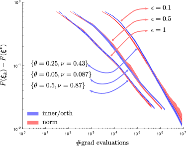
(A) Cases: $\#1$, $\#2$, and $\#3$

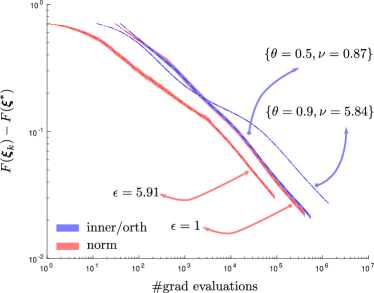
(B) Cases: $\#3$ and $\#4$

Figure 2. The objective function in (36): optimality gap versus total cost.

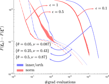
(A) Cases: $\#1$, $\#2$, and $\#3$

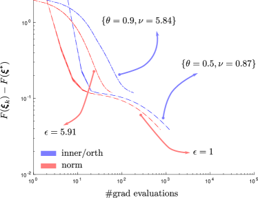
(B) Cases: $\#3$ and $\#4$

Figure 3. The objective function in (38): optimality gap versus total cost.

The equivalence in terms of both convergence and cost is clear from Figure 2LABEL:sub@fg:1.a for the first objective function (36) for the parameter cases $\#1$, $\#2$, and $\#3$. The equivalence does not hold, however, for the case $\#4$. Furthermore, from Figure 3 we deduce that the equivalence does not hold in any of the considered cases for objective function (38). This is because, for the equivalence between these batch size selection approaches, both expressions (33) and (34) must hold at every iteration of the SGD method. To achieve this, and hence be equivalent selection strategies, the parameters $\theta$ and $\nu$ should thus vary along the optimization path.

6. Acknowledgments

This work was partially supported by the KAUST Office of Sponsored Research (OSR) under Award numbers URF$/1/2281-01-01$, URF$/1/2584-01-01$ in the KAUST Competitive Research Grants Program Round 8, the Alexander von Humboldt Foundation.

7. Conclusions

In this study, we demonstrate that the norm and inner product/orthogonality tests are theoretically equivalent in terms of cost and convergence rates. We demonstrate the equivalence of our theoretical predictions by illustrating them in a simple stochastic optimization problem.

8. Data availability statement

The data that support the findings of this study are available from the corresponding author upon resonable request.

8.1. Conflict of interest

The authors have no conflicts to disclose.

References

- [1] Raghu Bollapragada, Richard Byrd, and Jorge Nocedal. Adaptive sampling strategies for stochastic optimization. SIAM Journal on Optimization, 28(4):3312–3343, 2018.
- [2] Richard G Carter. On the global convergence of trust region algorithms using inexact gradient information. SIAM Journal on Numerical Analysis, 28(1):251–265, 1991.
- [3] Richard H Byrd, Gillian M Chin, Jorge Nocedal, and Yuchen Wu. Sample size selection in optimization methods for machine learning. Mathematical programming, 134(1):127–155, 2012.
- [4] Fatemeh S Hashemi, Soumyadip Ghosh, and Raghu Pasupathy. On adaptive sampling rules for stochastic recursions. In Proceedings of the Winter Simulation Conference 2014, pages 3959–3970. IEEE, 2014.
- [5] Coralia Cartis and Katya Scheinberg. Global convergence rate analysis of unconstrained optimization methods based on probabilistic models. Mathematical Programming, 169(2):337–375, 2018.
- [6] Andre Carlon, Luis Espath, Rafael Lopez, and Raul Tempone. Multi-iteration stochastic optimizers. arXiv preprint arXiv:2011.01718, 2020.