Violent nonlinear collapse in the interior of charged hairy black holes

Abstract

We construct a new one-parameter family indexed by $\epsilon$ of two-ended, spatially-homogeneous black hole interiors solving the Einstein–Maxwell–Klein–Gordon equations with a (possibly zero) cosmological constant $\Lambda$ and bifurcating off a Reissner–Nordström-(dS/AdS) interior ($\epsilon=0$). For all small $\epsilon\neq 0$, we prove that, although the black hole is charged, its terminal boundary is an everywhere-spacelike Kasner singularity foliated by spheres of zero radius $r$.

Moreover, smaller perturbations (i.e. smaller $|\epsilon|$) are more singular than larger one, in the sense that the Hawking mass and the curvature blow up following a power law of the form $r^{-O(\epsilon^{-2})}$ at the singularity $\{r=0\}$. This unusual property originates from a dynamical phenomenon – violent nonlinear collapse – caused by the almost formation of a Cauchy horizon to the past of the spacelike singularity $\{r=0\}$. This phenomenon was previously described numerically in the physics literature and referred to as “the collapse of the Einstein–Rosen bridge”.

While we cover all values of $\Lambda\in\mathbb{R}$, the case $\Lambda<0$ is of particular significance to the AdS/CFT correspondence. Our result can also be viewed in general as a first step towards the understanding of the interior of hairy black holes.

1 Introduction

The no-hair conjecture is a well-known statement in the Physics literature, broadly claiming that all stationary black holes are solely described by their mass, angular momentum and charge (namely they belong to the Kerr–(Newman) or the Reissner–Nordström family), see the review [15] and references therein. In (electro)-vacuum, celebrated uniqueness theorems [10, 31, 38, 39, 54] preclude the existence of asymptotically flat “hairy” black holes. However, there exists a plethoric literature on hairy black holes for relatively exotic matter models: Arguably the most emblematic known hairy black holes are static solutions coupled with non-abelian gauge theories, satisfying the Einstein–Yang–Mills equations [6, 7, 23, 56] or the Einstein–Yang–Mills equations coupled with a Higgs or Dilaton field [7, 22, 57].

In the present study, we consider a typical matter model, the Einstein–Maxwell–Klein–Gordon equations, with a cosmological constant $\Lambda\in\mathbb{R}$, and a scalar field $\phi$ obeying the linear Klein–Gordon equation with mass $m^{2}\in\mathbb{R}-\{0\}$:

$$Ric_{\mu\nu}(g)-\frac{1}{2}R(g)g_{\mu\nu}+\Lambda g_{\mu\nu}=\mathbb{T}^{EM}_{\mu\nu}+\mathbb{T}^{KG}_{\mu\nu},$$ (1.1)

$$\mathbb{T}^{EM}_{\mu\nu}=2\left(g^{\alpha\beta}F_{\alpha\nu}F_{\beta\mu}-\frac{1}{4}F^{\alpha\beta}F_{\alpha\beta}g_{\mu\nu}\right),\hskip 19.91692pt\nabla^{\mu}F_{\mu\nu}=0,$$ (1.2)

$$\mathbb{T}^{KG}_{\mu\nu}=2\left(\nabla_{\mu}\phi\nabla_{\nu}\phi-\frac{1}{2}(g^{\alpha\beta}\nabla_{\alpha}\phi\nabla_{\beta}\phi+m^{2}|\phi|^{2})g_{\mu\nu}\right),$$ (1.3)

$$g^{\mu\nu}\nabla_{\mu}\nabla_{\nu}\phi=m^{2}\phi.$$ (1.4)

A uniqueness result of Bekenstein [5] precludes the existence of asymptotically flat ($\Lambda=0$) hairy black holes for the above system (at least when $m^{2}\geq 0$). However, there has been recent significant interest in asymptotically AdS static hairy black holes when $\Lambda<0$, in connection with the AdS/CFT correspondence [1, 9, 26, 27, 29, 30]. In our main theorem below, we will consider the subject under a dynamical perspective and study rigorously the time-evolution of characteristic initial data consisting in a constant scalar field $\phi\equiv\epsilon$ of small amplitude $\epsilon\neq 0$ on a two-ended event horizon. The resulting spacetime is a one-parameter family bifurcating from the Reissner–Nordström-(dS/AdS) interior metric, which we interpret as the interior region of a charged and static hairy black hole. We will however limit our study to the black hole interior and not concern ourselves with the construction of the asymptotically AdS black hole exterior (see Figure 4), since we do not want to impose the sign of the cosmological constant in the present work.

The resulting family of metrics $g_{\epsilon}$ we construct are charged $\epsilon$-perturbations of the Reissner–Nordström-(dS/AdS) interior, but surprisingly do not admit a Cauchy horizon; instead, their singularity is everywhere spacelike (Figure 1).

Furthermore, we show that the evolution problem obeys highly nonlinear dynamics leading to a more violent singularity than expected. Finally, we also address the limit $\epsilon\rightarrow 0$, and show that it is non-unique; moreover, convergence is not uniform, and only holds in a very rough topology given by the Bounded Mean Oscillations norm (BMO norm).

Theorem I.

[Rough version] Fix the following characteristic initial data on bifurcating event horizons $\mathcal{H}^{+}_{1}\cup\mathcal{H}^{+}_{2}$:

$$\phi\equiv\epsilon,$$ (1.5)

$$g=g_{RN},$$ (1.6)

where $g_{RN}$ is the Reissner–Nordström-(dS/AdS) metric ($g_{RN}$) with sub-extremal parameters $(M,e,\Lambda)$. The Maximal Globally Hyperbolic Development $(\mathcal{M}_{\epsilon},g_{\epsilon})$ of this data is a spatially-homogeneous spacetime with topology $\mathbb{R}\times\mathbb{S}^{2}$.

Then, for almost every $(M,e,\Lambda,m^{2})$, there exists $\epsilon_{0}(M,e,\Lambda,m^{2})>0$ such that for all $0<|\epsilon|<\epsilon_{0}$, the spacetime $(\mathcal{M}_{\epsilon},g_{\epsilon})$ ends at a spacelike singularity $\mathcal{S}:=\{r=0\}$, where $r$ is the area-radius of the $\mathbb{R}\times\mathbb{S}^{2}$ cylinder. Moreover:

1. Almost formation of a Cauchy horizon: $g_{\epsilon}$ is uniformly close to Reissner–Nordström-(dS/AdS) locally (in Reissner–Nordström-(dS/AdS) time) and moreover $g_{\epsilon}$ converges weakly to Reissner–Nordström-(dS/AdS) as $\epsilon\rightarrow 0$.

2. Singular power-law inflation: the Hawking mass $\rho$ and the Kretschmann scalar $\mathfrak{K}$ blow up at $\mathcal{S}:=\{r=0\}$ as:

   $$\begin{split}\rho(r)\approx r^{-b_{-}^{-2}\epsilon^{-2}+O(\epsilon^{-1})},\hskip 14.22636pt\mathfrak{K}(r)\approx r^{-2b_{-}^{-2}\epsilon^{-2}+O(\epsilon^{-1})},\end{split}$$ (1.7)

   and we call $b_{-}(M,e,\Lambda,m^{2})\neq 0$ the resonance parameter. $\approx$ means equivalent as $r\rightarrow 0$, up to a constant.

3. Kasner-type behavior: near the singularity $\mathcal{S}:=\{r=0\}$, $g_{\epsilon}$ is uniformly close to a Kasner-like metric $\tilde{g}_{\epsilon}^{Kas}$:

   $$\tilde{g}_{\epsilon}^{Kas}=-d\tilde{\tau}^{2}+\tilde{\tau}^{2(1-4b_{-}^{2}\epsilon^{2})+O(\epsilon^{3})}d\rho^{2}+\tilde{\tau}^{4b_{-}^{2}\epsilon^{2}+O(\epsilon^{3})}\cdot r_{-}^{2}\cdot(d\theta^{2}+\sin^{2}(\theta)d\psi^{2}),\$$ (1.8)

   $$\phi(\tilde{\tau})=2b_{-}\cdot[\epsilon+O(\epsilon^{2})]\cdot\log(\tilde{\tau}^{-1}),$$ (1.9)

   where $r_{-}(M,e,\Lambda)>0$ is the radius of the Cauchy horizon of the unperturbed metric ($g_{RN}$)$=g_{\epsilon=0}$.

4. $BMO$ convergence: near the singularity $\mathcal{S}:=\{r=0\}$, $g_{\epsilon}$ converges to Minkowski in the $BMO$ norm as $\epsilon\rightarrow 0$.

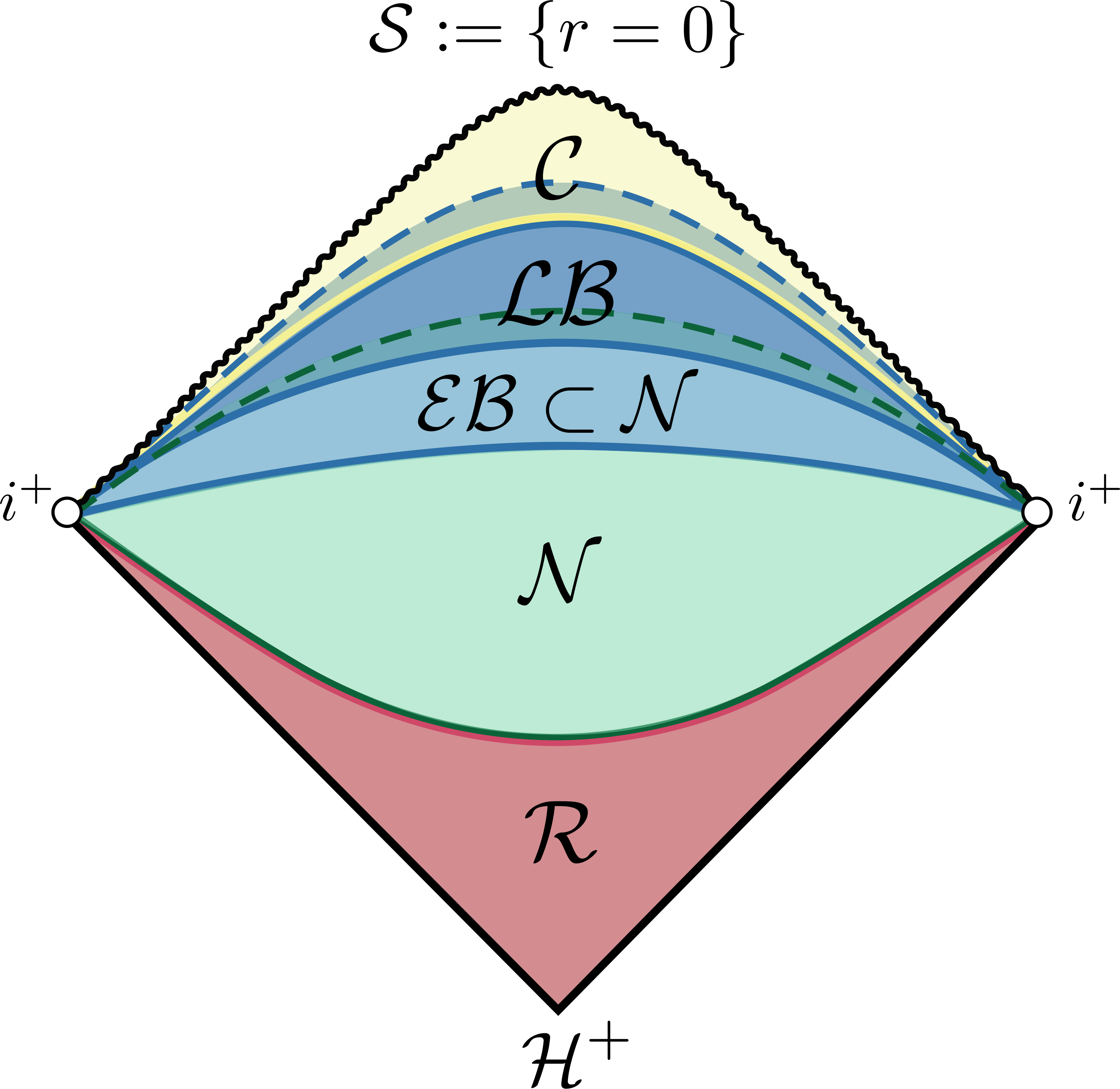
Figure 1: Penrose diagram of $g_{\epsilon}$ from Theorem I, where $\mathcal{S}=\{r=0\}$ is a spacelike singularity. The spacetime regions $\mathcal{R}$, $\mathcal{N}$, $\mathcal{EB}$, $\mathcal{LB}$ and $\mathcal{C}$ are introduced in Section 1.8. Note that $\mathcal{LB}$ overlaps with $\mathcal{C}$ and $\mathcal{N}$ and $\mathcal{EB}\subset\mathcal{N}$.

We emphasize that we do not fix the sign of $\Lambda$, or of $m^{2}$: if $\Lambda=0$ (respectively $\Lambda>0$, $\Lambda<0$), the spacetime metric $g_{\epsilon=0}$ from which $g_{\epsilon}$ bifurcates is a Reissner–Nordström (respectively RN-de-Sitter, RN-anti-de-Sitter) interior metric.

We now make a few essential remarks on our spacetime $(\mathcal{M}_{\epsilon},g_{\epsilon})$, and announce the outline of the introduction:

• If we consider instead black holes solutions of (1.1)–(1.4) relaxing to Reissner–Nordström, namely if instead of (1.5), we have the following non-hairy behavior of the scalar field

  $$\phi\rightarrow 0\text{ towards }i^{+}\text{ in the black hole exterior,}$$

  then the black hole interior does admit a Cauchy horizon, in complete contrast to the spacetime $(\mathcal{M}_{\epsilon},g_{\epsilon})$ of Theorem I, see Section 1.1 and Figure 2.

• Asymptotically AdS black holes play an important role in AdS/CFT, in connection to two of the most celebrated problems in the quantum aspects of gravity: the information paradox [32, 33, 28] on the one hand, and the probing of the singularity at the black hole terminal boundary on the other hand [27, 29, 30] (see Section 1.2). For both problems, many standard results in AdS/CFT (like the computations of entanglement entropy [28]) are considered on the Reissner–Nordström-AdS spacetime, which is very specific in that it has a Cauchy horizon, contrary to $g_{\epsilon}$. It would be interesting to examine these results on the more general spacetime $(\mathcal{M}_{\epsilon},g_{\epsilon})$ constructed in Theorem I.

• Although $g_{\epsilon}$ has a spacelike singularity, a Cauchy horizon almost forms, i.e. $g_{\epsilon}$ is close to Reissner–Nordström-(dS/AdS) for large intermediate times (at which a Reissner–Nordström metric would be “close to its Cauchy horizon”). Moreover, we have weak convergence of $g_{\epsilon}$ to Reissner–Nordström-(dS/AdS), see Section 1.3.

• The almost formation of the Cauchy horizon dramatically impacts the singularity structure and is responsible for what we call violent nonlinear collapse, reflected by the $r^{-b_{-}^{-2}\epsilon^{-2}}$ power-law inflation rates from 1.7. Such singular rates (note that $\epsilon^{-2}\rightarrow\infty$, as $\epsilon\rightarrow 0$) conjecturally do not occur for hairy perturbations of Schwarzschild-(dS/AdS), see Section 1.4.

• The other effect of violent nonlinear collapse is to make $g_{\epsilon}$ uniformly close (near the singularity) to a Kasner metric (see Section 1.5) of exponents $(1-4b_{-}^{2}\epsilon^{2}+O(\epsilon^{3}),\ 2b_{-}^{2}\epsilon^{2}+O(\epsilon^{3}),\ 2b_{-}^{2}\epsilon^{2}+O(\epsilon^{3}))$. Note that an exact Kasner metric of exponents $(1-4b_{-}^{2}\epsilon^{2},\ 2b_{-}^{2}\epsilon^{2},\ 2b_{-}^{2}\epsilon^{2})$ (recall that $b_{-}(M,e,\Lambda,m^{2})\neq 0$) converges (locally) to Minkowski in $BMO$ norm, but not uniformly as $\epsilon\rightarrow 0$, which is consistent with statement iv of Theorem I.

• In Section 1.6, we discuss other results and analogies between $g_{\epsilon}$ and hairy black holes for other matter models.

• The author hopes that the present study will pave the way towards other interesting problems such as

  1. Constructing a static, asymptotically AdS black hole exterior matching with the interior metric $g_{\epsilon}$.

  2. Understanding the stability of the metric $g_{\epsilon}$ with respect to non-spatially homogeneous perturbations.

  3. Understanding the singularity inside rotating (charged or uncharged) hairy black holes.

  4. Studying similar models which admit BKL-type oscillations, a topic of great importance in cosmology.

  For further developments on the above problems, we refer the reader to Section 1.7.

• Concerning the proof, we want to emphasize two important aspects (see Section 1.8 for more details):

  1. The importance of distinguishing different time scales, in particular short times in which Reissner–Nordström-(dS/AdS) enjoys Cauchy stability, intermediate times where a typical blue-shift instability kicks in and late times where the nonlinearity dominates and monotonicity takes over, leading to collapse to $\{r=0\}$.

  2. We exploit a linear instability [40] for the Klein–Gordon equation on Reissner–Nordström-(dS/AdS). This instability is important at early/intermediate times and relies on a scattering resonance (absent in the case $m^{2}=\Lambda=0$) giving $b_{-}\neq 0$, that occurs for almost every (but not all) parameters $(M,e,\Lambda,m^{2})$.

1.1 Comparison with non-hairy black holes relaxing to Reissner–Nordström

Dafermos–Luk proved in [20] the stability of Kerr’s Cauchy horizon with respect to vacuum perturbations relaxing to Kerr at a fast, integrable rate (consistent with the fast rates one would obtain in the exterior problem [17], [18]). For the model (1.1)–(1.4), the relaxation is conjectured to occur at a slower rate if $\Lambda=0$ (see the heuristics/numerics from [8], [45], [46]), which is a serious obstruction to asymptotic stability, even in spherical symmetry. Nevertheless, the author proved that the Reissner–Nordström Cauchy horizon is stable with respect to spherically symmetric perturbations, providing they decay at a (slow) inverse polynomial relaxation rate consistent with the conjectures:

Theorem 1.1 ([58]).

Let regular spherically symmetric characteristic data on $\mathcal{H}^{+}\cup\underline{C}_{in}$, where $\mathcal{H}^{+}:=[1,+\infty)_{v}\times\mathbb{S}^{2}$, converging to a sub-extremal Reissner–Nordström-(dS/AdS) at the following rate: for some $s>\frac{1}{2}$ and for all $v\in\mathcal{H}^{+}$:

$$|\phi|(v)+|\partial_{v}\phi|(v)\lesssim v^{-s},$$ (1.10)

where $v$ is a standard Eddington–Finkelstein advanced time-coordinate. Then, restricting $\underline{C}_{in}$ to be sufficiently short, the future domain of dependence of $\mathcal{H}^{+}\cup\underline{C}_{in}$ is bounded by a Cauchy horizon $\mathcal{CH}^{+}$, namely a null boundary emanating from $i^{+}$ and foliated by spheres of strictly positive area-radius $r$, as depicted in Figure 2.

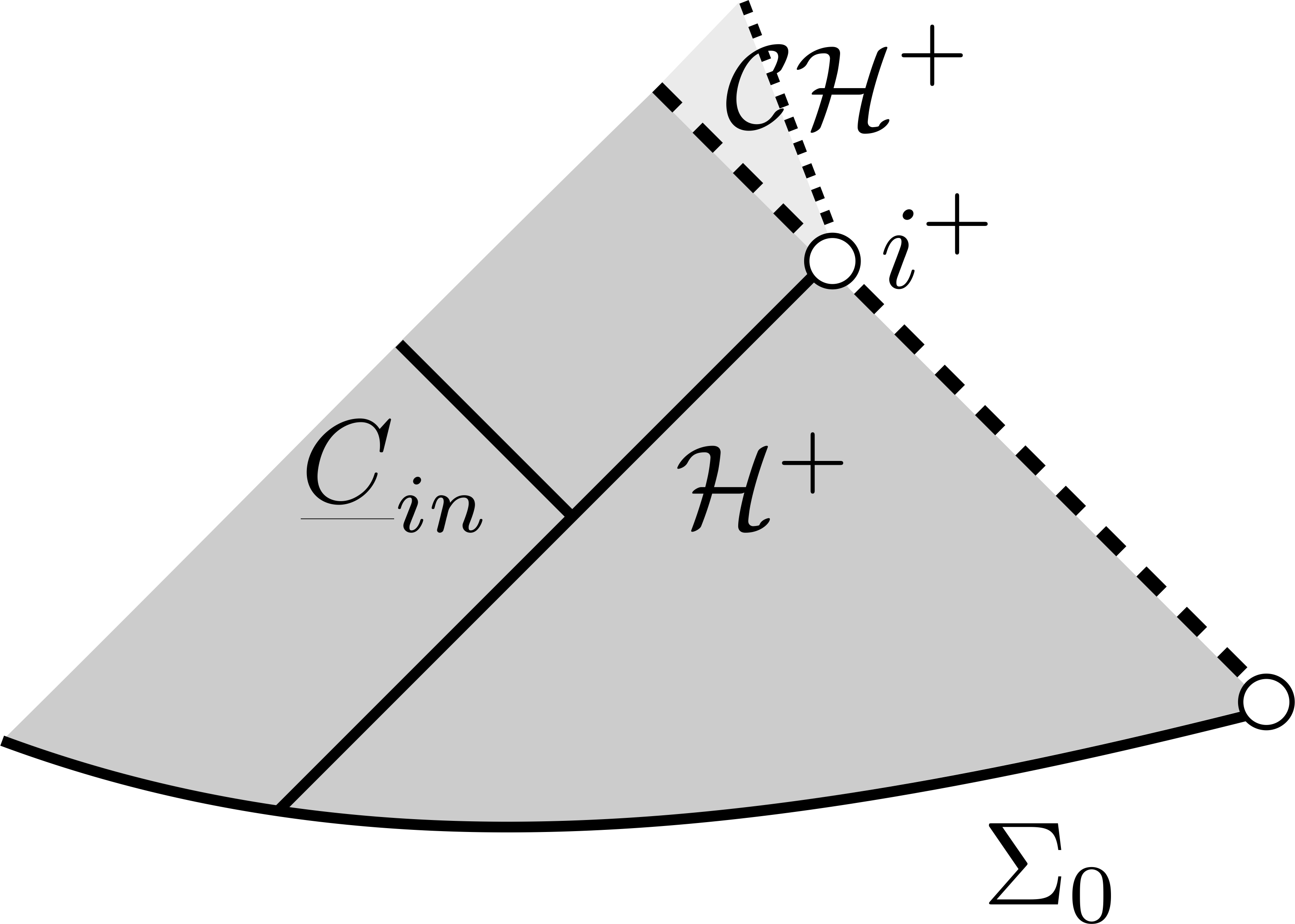
Figure 2: Penrose diagram of the spacetime corresponding to Theorem 1.1

• Theorem 1.1 stands in complete contrast with Theorem I: to summarize, the Cauchy horizon is stable if $\phi$ decays to zero (even at a slow rate as in (1.10)) but is unstable if $\phi\equiv\epsilon$ is small but does not decay.

• Note that for $\Lambda=0$ and asymptotically flat Cauchy data, since by [5], Reissner–Nordström is the only static solution of (1.1)–(1.4), it means that the decay of $\phi$ to $0$ indeed quantifies the relaxation of the black hole exterior towards a Reissner–Nordström metric. In a slight abuse of terminology, we will say that a (spherically symmetric) black hole relaxes to Reissner–Nordström when the scalar field $\phi$ tends to $0$ towards $i^{+}$ in black hole exterior.

• Note that the polynomial decay as in (1.10) is conjecturally sharp in the exterior if $\Lambda=0$, but not if $\Lambda>0$ because the decay is exponential [35]; moreover (1.10) is not satisfied if $\Lambda<0$, as the decay is logarithmic [37].

• If we assume integrable decay, i.e. $s>1$ (an unrealistic assumption if $\Lambda=0$, in view of the conjectured rates in the exterior), then we prove in [58] that the metric is continuously extendible at the Cauchy horizon. Under similar assumptions, Dafermos–Luk reached the same conclusion for perturbations of Kerr [20] without symmetry: since the integrable decay $s>1$ becomes a realistic assumption in the vacuum [18, 19, 43], the result of Dafermos–Luk [20] also falsifies the $C^{0}$-formulation of Strong Cosmic Censorship (by means of decay).

• Nevertheless, if $\frac{1}{2}<s\leq 1$, there is a large class of $\phi$-data obeying (1.10) such that the Cauchy horizon exists, but admits a novel null contraction singularity that renders the metric $C^{0}$-inextendible, and $\phi$ is unbounded in amplitude [41, 42]. However, uniform boundedness and continuous extendibility of the metric and $\phi$ hold for a sub-class of oscillating event horizon data, as proven in [41]. Since these oscillations at the event horizon are conjectured to be generic [36, 46], the work [41] also falsifies the $C^{0}$-formulation of Strong Cosmic Censorship in spherical symmetry by means of the oscillations of the perturbation (as opposed to by means of decay).

• If we assume an averaged version of (1.10) as a lower bound (still consistent with the conjectured rates) then we proved in [58, 61] that the curvature blows up at the Cauchy horizon and that mass inflation occurs (i.e. the Hawking mass blows up): this shows that the metric is (future) $C^{2}$-inextendible [61]. This statement is called the $C^{2}$ version of the Strong Cosmic Censorship conjecture, which is thus true for this matter model.

• Theorem 1.1 is a local result, which is independent of the topology of the Cauchy data. It turns out that solutions of (1.1)–(1.4) with $F\neq 0$ in spherical symmetry are constrained to have two-ended data topology $\mathbb{R}\times\mathbb{S}^{2}$, a setting which is not realistic to study astrophysical gravitational collapse (but may be in other settings, see Section 1.2). In fact, Theorem 1.1 and all the results claimed in this section were originally proven for the Einstein–Maxwell–Klein–Gordon system where the scalar field $\phi$ is also allowed to be charged, see [58], [61]. Unlike model (1.1)–(1.4), this charged model allows for one-ended data with topology $\mathbb{R}^{3}$ admitting a regular center and provides an acceptable model to study spherical collapse as a global phenomenon. The one-ended collapse case brings a striking conclusion: under the above assumptions, while a Cauchy horizon $\mathcal{CH}^{+}$ is present near $i^{+}$ (in the domain of dependence of $\underline{C}_{in}$, see Figure 2), it breaks down globally and a crushing singularity forms near the center, as we prove in [60].

1.2 Boundary value problem and potential applications to AdS/CFT

Two-ended stationary black holes (“eternal”) play a pivotal role in the celebrated Anti-de-Sitter/Conformal Field Theory correspondence [48], see for instance [49, 63]. In the AdS/CFT dictionary, charged black holes correspond thermodynamically to the Grand Canonical Ensemble of $N$ holographic theories at the boundary for large $N$ [11, 34].

One important open problem regarding the quantum aspects of gravity is the information paradox resulting from the apparent loss of information due to the quantum evaporation of black holes by Hawking radiation [32, 33]. Recently, the quantum concept of entanglement entropy [28] was used in an approach [53] to explain this paradox. Most computations in this context are, however, made on the Reissner–Nordström-AdS electro-vacuum solution, which is highly non-generic, and moreover its terminal boundary is a smooth Cauchy horizon $\mathcal{CH}^{+}_{A}\cup\mathcal{CH}^{+}_{B}$ (see Figure 3).

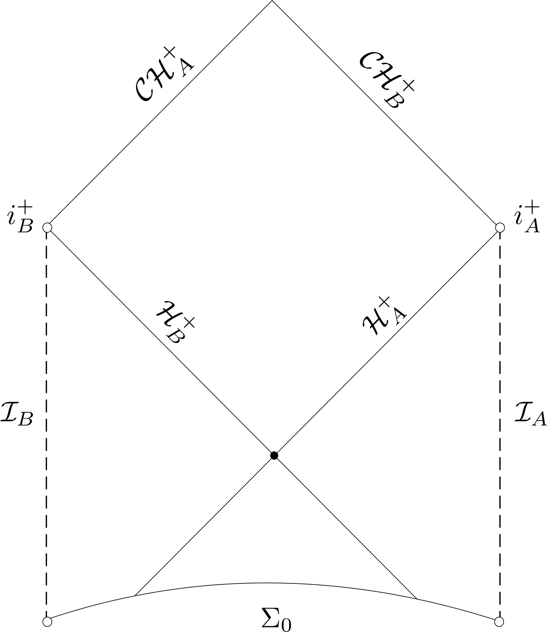
Figure 3: Penrose diagram of the Reissner–Nordström-AdS spacetime

In complete contrast, the terminal boundary of our charged hairy black holes $g_{\epsilon}$ from Theorem I is not a Cauchy horizon, but a spacelike singularity $\mathcal{S}$ instead (compared with Figure 1). It would be interesting to construct a static, asymptotically AdS black hole exterior corresponding to $g_{\epsilon}$ and carry out the computations of standard quantum quantities, such as the entanglement entropy, in this setting. The metric asymptotics we derive (see Theorem 3.1 and below) will likely be crucial for this task.

Another fundamental problem is the understanding of quantum effects near the singularity located at the terminal boundary of a black hole. As it turns out, the interior of asymptotically AdS black holes provides a simplified model to understand these effects; motivated by these considerations, Hartnoll et al. [27, 29, 30] studied numerically the interior of hairy black holes for various charged/uncharged matter models, and discovered a wealth of singularities (see Section 1.6). Charged hairy black holes with asymptotically AdS asymptotics are especially studied in the numerical work [29]: The interior part of these black holes corresponds to $g_{\epsilon}$ from Theorem I, see Section 1.6.1 for details.

Lastly, we mention a soft argument in [29] ruling out smooth Cauchy horizons (in particular, assuming a finite scalar field $\phi$), though in principle the result in [29] would still be consistent with having a singular Cauchy horizon (where the scalar field $\phi$ or its derivatives blow up for instance, even if the metric itself is smooth).

1.3 Almost formation of a Cauchy horizon and stability for intermediate times

For the purpose of this discussion, we define a time coordinate $s$ on $g_{\epsilon}$ by 2.32. On Reissner–Nordström-(dS/AdS),
$s$ coincides with the $r^{*}$-tortoise coordinate: in particular, $s=r^{*}\in\mathbb{R}$ and $\{s=+\infty\}$ is the Cauchy horizon, $\{s=-\infty\}$ is the event horizon. The statements (Theorem 3.1 and Theorem 3.2) we prove can be summarized as:

1. the spacetime $\mathcal{M}_{\epsilon}$ corresponds to $s\in(-\infty,s_{\infty}(\epsilon))$, ending at $\mathcal{S}=\{r=0\}=\{s_{\infty}(\epsilon)\}$ and $s_{\infty}(\epsilon)\simeq\epsilon^{-2}<+\infty$.

2. $g_{\epsilon}$ is uniformly close to the Reissner–Nordström-(dS/AdS) metric ($g_{RN}$) in amplitude for all $s\ll\epsilon^{-2}$.

3. The derivatives of the $g_{\epsilon}$ are uniformly close to the derivatives of $g_{RN}$ for all $s\ll\log(\epsilon^{-1})$.

4. The derivatives of the $g_{\epsilon}$, in particular the Hawking mass, become arbitrarily large for $\log(\epsilon^{-1})\ll s\lesssim\epsilon^{-2}$.

5. $g_{\epsilon}$ converges in the sense of distributions $\mathcal{D}^{\prime}(\mathbb{R}_{s})$ to the Reissner–Nordström-(dS/AdS) metric ($g_{RN}$) as $\epsilon\rightarrow 0$.

6. $g_{\epsilon}$ does not converge uniformly to ($g_{RN}$), or in any Lebesgue space $L^{p}(\mathbb{R}_{s})$ for $p\geq 1$.

We interpret statement 2 as the almost formation of a Cauchy horizon, as $s$ is allowed to be larger than any $\epsilon$-independent constant, which, on Reissner–Nordström-(dS/AdS), corresponds to being close to the Cauchy horizon.

Note that we roughly have three regions (see Section 1.8 for details): $s\ll\log(\epsilon^{-1})$, where Cauchy stability prevails in the $C^{1}$ norm; $\log(\epsilon^{-1})\ll s\ll\epsilon^{-2}$, where $C^{0}$ stability still holds, but a $C^{1}$ blow-up, characteristic of the blue-shift instability, occurs; and lastly a region $s\simeq\epsilon^{-2}$ where the spacelike singularity forms, see Section 1.5.

Remark 1.1.

Note that the convergence in distributions from statement 5 is specifically expressed in the $s$ coordinate system (defined in (2.32)); therefore, it does not contradict the convergence to Minkowski (statement iv of Theorem I) which is valid in a Kasner-type coordinate $\tilde{\tau}$ (see (1.8)) that differs significantly from $s$ in the $\epsilon\rightarrow 0$ limit.

1.4 Violent nonlinear collapse and strength of the spacelike singularity

Despite the weak stability up to large intermediate times of Reissner–Nordström-(dS/AdS), a spacelike singularity forms at late times $s\simeq\epsilon^{-2}$. We discuss the strength of this singularity, and compare it to the Schwarzschild metric:

$$g_{S}:=-(1-\frac{2M}{r})dt^{2}+(1-\frac{2M}{r})^{-1}dr^{2}+r^{2}[d\theta^{2}+\sin(\theta)^{2}d\varphi^{2}]. g_{S}$$ ()

On the Schwarzschild metric ($g_{S}$), $r$ is also the area-radius and the Hawking mass is constant equal to $M>0$. We argue that the singularity $\mathcal{S}=\{r=0\}$ on $g_{\epsilon}$ is “more singular” than $\{r=0\}$ on ($g_{S}$), which justifies our denomination violent nonlinear collapse (we explain the origin of “nonlinear” later in the section) for four reasons:

1. The Hawking mass $\rho$ on $g_{\epsilon}$ blows up as a power-law $r^{-b_{-}^{-2}\cdot\epsilon^{-2}}$ at $r=0$, as opposed to being constant on ($g_{S}$).

2. The Kretchsmann scalar $\mathfrak{K}:=R_{\alpha\beta\gamma\delta}R^{\alpha\beta\gamma\delta}$ blows up like $r^{-2b_{-}^{2}\cdot\epsilon^{-2}}$ as opposed to blowing-up like $r^{-6}$ on ($g_{S}$).

3. The quantity $r^{6}\rho^{-2}\mathfrak{K}\simeq\epsilon^{-4}$ is finite on $g_{\epsilon}$ (as on ($g_{S}$)) but becomes arbitrarily large for arbitrarily small $|\epsilon|$.

4. The spacetime volume of $\{r\geq r_{0},\ 0\leq t\leq 1\}$ is approximately $r_{0}^{b_{-}^{-2}\cdot\epsilon^{-2}}$ for small $r_{0}$, as opposed to $r^{3}_{0}$ on ($g_{S}$).

To go beyond the heuristics of this section, we refer to Theorem 3.1 for the precise estimates that we prove.

It is also interesting to compare $g_{\epsilon}$ to spherically symmetric solutions in Christodoulou’s model (i.e. (1.1)-(1.4) with $F\equiv 0$, $m^{2}=\Lambda=0$) constructed in [13, 14]; such spacetimes converge to ($g_{S}$) towards $i^{+}$ and admit a spacelike singularity. It has been proven recently [2], [3] that, on these spacetimes, $\mathfrak{K}$ and $\rho$ blow-up like $r^{-\alpha(t)}$ with a time-dependent rate $\alpha(t)$ converging to the Schwarzschild values as $t\rightarrow+\infty$, respectively $6$ and $0$.

In view of this, the truly surprising fact is not the power-law blow up of $\rho$, but the $\epsilon^{-2}$-rate, which tends to $+\infty$ as $|\epsilon|\rightarrow 0$. Naively, one may expect that an $\epsilon$-perturbation of ($g_{RN}$) will give rise to $O(\epsilon)$ rates at the very least, allowing to recover ($g_{RN}$) in the (strong) limit but we obtain a singular limit instead, caused by the nonlinearity.

To understand, it is useful look to at the linear equation $\Box_{g_{S}}\psi=0$. Solutions blow-up at $r=0$ (see [25]) as:

$$\psi(r,t)\approx A(t)\cdot\log(r^{-1}).$$

For constant data $\psi\equiv\epsilon$ on the event horizon, we get $A(t)=C(M)\cdot\epsilon$, consistent with the linearity of the equation.

However, in the evolution $(g_{\epsilon},\phi_{\epsilon}=\epsilon)$ of the data of Theorem I we have, near the singularity $\mathcal{S}=\{r=0\}$:

$$\phi_{\epsilon}(r)\simeq\epsilon^{-1}\cdot\log(r^{-1}),$$ (1.11)

a radically different rate ! The main explanation behind (1.11) is a nonlinear estimate that we prove on $g_{\epsilon}$:

$$\frac{dr}{ds}\simeq-\epsilon^{2}\cdot r^{-1},$$ (1.12)

to be compared with $\frac{dr}{ds}\approx-M\cdot r^{-1}$ on ($g_{S}$) (with the same $s$ defined by (2.32)). The striking fact, is that (1.12) is a remnant of the Reissner–Nordström Cauchy horizon stability for intermediate times (the phenomenon we explained in Section 1.3) ! This explains our claim that the violent nonlinear collapse phenomenon only occurs for nonlinear perturbations of charged black holes, and not perturbations of Schwarzschild. The numerics of [27], where data are set as in Theorem I replacing ($g_{RN}$) by ($g_{S}$) (equivalently assuming $F\equiv 0$), tend to confirm this expectation.

Further details on this nonlinear collapse dynamics and the role of the different actors are given in Section 1.8.

1.5 Kasner-like behavior and convergence in scale-invariant spaces $L^{\infty}$/$BMO$

We recall the Kasner metric, a solution of the Einstein-scalar-field system i.e. (1.1)-(1.4) with $F\equiv 0$, $m^{2}=0$:

$$g_{Kas}=-d\tilde{\tau}^{2}+\tilde{\tau}^{2p_{rad}}d\rho^{2}+\tilde{\tau}^{2p_{x}}dx^{2}+\tilde{\tau}^{2p_{y}}dy^{2},\hskip 14.22636pt\phi(\tilde{\tau})=p_{\phi}\cdot\log(\tilde{\tau}^{-1});$$ (1.13)

$$p_{rad}+p_{x}+p_{y}=1,\hskip 28.45274ptp_{rad}^{2}+p_{x}^{2}+p_{y}^{2}+2p_{\phi}^{2}=1.$$ (1.14)

The Kasner solution has been used in cosmology as a model of anisotropic Big Bang singularity, in the presence of a so-called stiff fluid (here the scalar field $\phi$). In a recent breakthrough, Fournodavlos–Rodnianski–Speck [24] proved that, under a sub-criticality condition on the exponents from (1.14), the family (1.13) is stable against perturbations, with no symmetry assumptions and that the near-singularity dynamics are dominated by monotonic blow-up.

Remark 1.2.

Relation 1.14 may seem unfamiliar, because of the factor $2$ in front of $p_{\phi}^{2}$. This is due to our definition in (1.3) (adopted in the majority of works in the black hole interior [13, 14, 16, 44, 47] …), as opposed to the standard definition in cosmology where the factor $2$ is absent in (1.3), see for instance [24].

Anisotropic Kantowski–Sachs metrics

We study spatially-homogeneous metrics of the form

$$g_{\epsilon}=-\Omega^{2}(s)(ds^{2}-dt^{2})+r^{2}(s)d\Sigma_{k},$$ (1.15)

where $d\Sigma_{k}$ is the standard metric on $\Sigma_{k}$ the 2-surface of sectional curvature $k\in\{-1,0,1\}$ ($\mathbb{H}^{2}$, $\mathbb{T}^{2}$, $\mathbb{S}^{2}$ respectively) and $r$ is a scalar function called the area-radius, which is geometrically well-defined using the symmetry class. The underlying topology, which is $\mathbb{R}^{1+1}\times\Sigma_{k}$, is irrelevant to the proof of our result. In case $\Sigma_{k}=\mathbb{S}^{2}$, such metric are called Kantowski–Sachs cosmologies and are used to model an anisotropic but spatially homogeneous cosmology.

Monotonic blow-up due to the scalar field

Our collapse from an almost Cauchy horizon to a spacelike singularity is caused by purely nonlinear dynamics driven by monotonicity. Specifically, the Einstein equations ((2.23)) give a relation where the scalar field dominates and acts as a monotonic source for the lapse $\Omega^{2}$ from (1.15):

$$\frac{d^{2}}{ds^{2}}\left[\log(\Omega^{2})\right](s)=-2(\frac{d\phi}{ds})^{2}+...$$ (1.16)

As we shall explain in Section 1.8, (1.16) gives rise to a Kasner-type behavior, as given right below, once the lower order terms $...$ have been quantitatively controlled. We emphasize however that the sharp asymptotics of the $-2(\frac{d\phi}{ds})^{2}$ are necessary for the proof (not only its sign!).

Uniform estimates near a (quasi)-Kasner metric

Note that, as stated, the Kasner exponents are constants, but there exists generalization of (1.13) where the exponents are allowed to depend on $x$, $y$ and $\rho$ (but not on $\tilde{\tau}$). Formally, our metric $g_{\epsilon}$, written as (1.8), corresponds (up to errors that converge uniformly to zero as $\epsilon\rightarrow 0$) to a Kasner metric of exponents $p_{rad}=1-4b_{-}^{2}\cdot\epsilon^{2}$, $p_{x}=p_{y}=2b_{-}^{2}\cdot\epsilon^{2}$, $p_{\phi}=2b_{-}\cdot\epsilon$ (up to a $O(\epsilon^{3})$ error), which satisfy (1.14) to order $O(\epsilon^{4})$. Nevertheless, the $O(\epsilon^{3})$ error are actually time-dependent (see Theorem 3.11), so (1.8) is not necessarily an exact Kasner metric (although the time-dependence in the Kasner exponents is lower order in $\epsilon$). Our uniform estimates are only valid in a Kasner-time coordinate $\tilde{\tau}$ (thus, do not contradict the convergence in distribution to Reissner–Nordström-(dS/AdS) in the other time coordinate $s$ from Section 1.3) defined so that the metric takes the following product form:

$$g_{\epsilon}=-d\tilde{\tau}^{2}+\underbrace{\Omega^{2}(\tilde{\tau})dt^{2}+r^{2}(\tilde{\tau})d\Sigma_{k}}_{\breve{g}},$$ (1.17)

where $\breve{g}$ does not involve $d\tilde{\tau}$. This form is often called the synchronous gauge (i.e. unitary lapse with zero shift).

Comparison between the Kasner time and the area-radius

The spacelike singularity $\mathcal{S}=\{r=0\}$ corresponds to $\{\tilde{\tau}=0\}$. Another consequence of the almost stability of the Reissner–Nordström-(dS/AdS) Cauchy horizon is an important discrepancy between the area-radius $r$ (from (1.15)) and the Kasner time $\tilde{\tau}$ (from (1.17)):

$$\tilde{\tau}(r)\approx(\frac{r}{r_{-}})^{\frac{\epsilon^{-2}}{2b_{-}^{2}}+O(\epsilon^{-1})},\ \text{or equivalently}\ r(\tilde{\tau})\approx r_{-}(M,e,\Lambda)\cdot\tilde{\tau}^{2b_{-}^{2}\epsilon^{2}+O(\epsilon^{3})}.$$

The above relation also explains immediately how we find Kasner exponents of the form $(1-O(\epsilon^{2}),\ O(\epsilon^{2}),\ O(\epsilon^{2}))$.

Convergence to Minkowski in the $BMO$ norm

The particular case where $p_{rad}=1$, $p_{x}=p_{y}=p_{\phi}=0$ in 1.13 corresponds (locally) to the Minkowski metric. If $(p_{rad},p_{x},p_{y},p_{\phi})=(1+\alpha_{rad}(\epsilon),\ \alpha_{x}(\epsilon),\ \alpha_{y}(\epsilon),\ \alpha_{\phi}(\epsilon))$, and $\alpha_{rad}(\epsilon)$, $\alpha_{x}(\epsilon)$, $\alpha_{y}(\epsilon)$, $\alpha_{\phi}(\epsilon)$ tend to $0$ as $\epsilon\rightarrow 0$, the corresponding Kasner metric (1.13) converges in $L^{p}([0,1]_{\tilde{\tau}})$ to Minkowski, for any $p<+\infty$. Although we want to show that $g_{\epsilon}$ converges to Minkowski as well, convergence in $L^{p}([0,1]_{\tilde{\tau}})$, while true (in particular, it follows from Theorem 3.3), is not entirely satisfactory for this purpose; we make the following observations to explain why and provide context:

1. We want convergence in a region of the form $\{\tilde{\tau}\ll\epsilon^{2}\}$; any other statement is hopeless: recall that for $\tilde{\tau}\approx 1$ (i.e. $s\approx 1$), the metric converges to Reissner–Nordström-(dS/AdS) (Section 1.3).

2. Convergence in $L^{p}([0,1]_{\tilde{\tau}})$ for any fixed $p<+\infty$ depends on the scaling of the coordinate $\tilde{\tau}$. Because integrating over $\{0<\tilde{\tau}\ll\epsilon^{2}\}$ provides extra $\epsilon$ factors, $L^{p}([0,1]_{\tilde{\tau}})$ convergence in this region is rather trivial.

3. Instead, we should work with a scale-invariant norm like $L^{\infty}$. $g_{\epsilon}$ is uniformly close to a Kasner metric near the singularity, but Kasner itself is not uniformly close to Minkowski: therefore, uniform convergence is false.

4. The Bounded-Mean-Oscillations space $BMO$ (see below), provides a scale-invariant norm, which is sometimes used as a substitute to $L^{\infty}_{loc}$. $BMO$ is a larger space containing $L^{\infty}_{loc}$, and most famously $\log(x)\in BMO([0,1])$.

5. The Kasner metric with exponents $(p_{rad},p_{x},p_{y},p_{\phi})=(1+\alpha_{rad}(\epsilon),\alpha_{x}(\epsilon),\ \alpha_{y}(\epsilon),\ \alpha_{\phi}(\epsilon))$ does converge quantitatively to Minkowski in the $BMO$ norm: this result can be obtained from an explicit computation.

Before closing this paragraph, we give the definition of $BMO([0,T])$ and note its scale-invariance; for all $\lambda>0$:

$$\|f\|_{BMO([0,T])}:=\sup_{0<a<b<T}\frac{\int_{a}^{b}\bigl{|}f(s)-\frac{\int_{a}^{b}f(w)dw}{b-a}\bigr{|}ds}{b-a}=\|f_{\lambda}\|_{BMO([0,\lambda T])},\hskip 14.22636ptf_{\lambda}(s):=f(\frac{s}{\lambda}).$$

To summarize Statement iii and Statement iv, we show that, schematically (see Theorem 3.3 for details):

$$(g_{\epsilon})_{\alpha\beta}=g_{Kas}+\mathfrak{E}^{unif}_{\alpha\beta}=m_{\alpha\beta}+E^{BMO}_{\alpha\beta},$$

where $g_{Kas}$ is formally (1.13) with Kasner parameters $(p_{rad},p_{x},p_{y},p_{\phi})=(1-4b_{-}^{2}\cdot\epsilon^{2},2b_{-}^{2}\cdot\epsilon^{2},2b_{-}^{2}\cdot\epsilon^{2},2b_{-}\cdot\epsilon)+O(\epsilon^{3})$, $m$ is the Minkowski metric, $\mathfrak{E}^{unif}_{\alpha\beta}$ converges to $0$ in $L^{\infty}([0,\epsilon^{2}]_{\tilde{\tau}})$ and $E^{BMO}_{\alpha\beta}$ converges to $0$ in $BMO([0,\epsilon^{2}]_{\tilde{\tau}})$.

Spatially-homogeneous perturbation of a Schwarzschild-(dS/AdS) spacetime

In Theorem I, we assume that the spacetime $g_{\epsilon=0}$ from which $g_{\epsilon}$ bifurcates is a Reissner–Nordström-(dS/AdS) metric, with a non-trivial Maxwell Field. A natural question is to ask what happens in the limiting case where the Maxwell field is zero, meaning when $g_{\epsilon=0}$ is the Schwarzschild-(dS/AdS) metric ($g_{S}$). Note that ($g_{S}$), under a coordinate change, corresponds to (1.13) with $\phi\equiv 0$ and exponents $(p_{rad},p_{x},p_{y})=(-\frac{1}{3},\frac{2}{3},\frac{2}{3})$. In the absence of a Maxwell field or angular momentum, there is no “mitigating factor” to collapse, and it is reasonable to expect that the metric will admit a spacelike singularity, and that as $\epsilon\rightarrow 0$, the space-time would converge in a weak sense to the unperturbed ($g_{S}$).

Remark 1.3.

If this expectation is true, then in the uncharged case, the stationary Schwarzschild-AdS black hole has a stable singularity $\mathcal{S}$ with respect to the hairy non-decaying perturbations $\phi$. Theorem I showed that, in contrast, this is not true in the charged case, since the Cauchy horizon of the Reissner–Nordström-AdS black hole is unstable.

While the uncharged analogue of $g_{\epsilon}$ is not covered in our work, numerics [27] support the above expectations. They also suggest the following important differences between $F\equiv 0$ and the charged case from Theorem I:

1. The Kasner exponents are bounded away from $0$ (with respect to $\epsilon$) in the uncharged case, and $p_{rad}<0$.

2. As a consequence, uncharged collapse is not violent (in the sense of Section 1.4), contrary to the charged case.

3. $\phi$ with data $\epsilon$ blows up at the singularity as $\phi\simeq\epsilon\cdot\log(r^{-1})$ as in the linear theory on ($g_{S}$) (see Section 1.4).

4. The background metric ($g_{S}$) is Cauchy-stable for small $\epsilon$, and there no bifurcation in the stability analysis.

We recall that points i, ii, iii, iv are in sharp contrast with Theorem I (the charged case), see Section 1.3 and 1.4.

1.6 Comparison with other matter models and other results in the interior

In this section, we mention prior results addressing the interior of a black hole that is not converging to Schwarzchild, Reissner–Nordström, or Kerr. Most of these works are based on either heuristics, or numerics.

1.6.1 Numerics on spatially homogeneous perturbations of the Reissner–Nordström-AdS interior

The metric $g_{\epsilon}$ from Theorem I was previously investigated in interesting numerical work [29]. The numerical results corroborate entirely Theorem I; they also consider the case of non-small perturbations (which are not covered by Theorem I) and suggest, that even in this case, a Kasner-like singularity forms. [29] was preceded by numerics in the uncharged case [27] (already mentioned in Section 1.5) and succeeded by numerics [30] studying spatially homogeneous perturbations of Reissner–Nordström-AdS in which the scalar field itself carries a charge (same model as in [58]-[61]). In the charged scalar field case, these numerics suggest intriguing intermediate time oscillations impacting the late-time Kasner singularity, see Section 1.7.

1.6.2 Spatially-homogeneous Einstein–Yang–Mills–Higgs interior solutions

The Einstein–$SU(2)$-(magnetic)-Yang–Mills are long-known to admit (non-singular) particle-like asymptotically flat solutions [4], [55], which are moreover static and spherically symmetric. An equally striking result is the mathematical construction [56] of a discrete, infinite family of (asymptotically flat) so-called colored black holes which thus falsify the no-hair conjecture for the $SU(2)$-Yang–Mills matter model (see also [6] for pioneering numerics).

The interior of such black holes is spatially homogeneous with topology $\mathbb{R}\times\mathbb{S}^{2}$, i.e.  corresponds to a Kantowski–Sachs cosmology analogous to our spacetime from Theorem I. Numerical studies in the interior of such black holes [23], [7] have highlighted oscillations and sophisticated dynamics, in which power law mass inflation/Kasner-type behavior alternates with the almost formation of a Cauchy horizon (analogous to the one discussed in Section 1.3).

The Einstein–$SU(2)$-Yang–Mills-Higgs model, in which a massive scalar field analogous to (1.4) is added, has also been studied numerically [23], [22], [56]. These studies suggest that the dynamics are drastically changed by the Higgs field which suppresses the oscillations, and the singularity is spacelike with a power-law mass inflation:

$$\phi(r)\approx\log(r^{-\lambda}),\hskip 14.22636pt\rho(r)\approx r^{-\lambda},$$ (1.18)

for some $\lambda>1$, which is consistent the behavior ((1.7), (1.11)) of $g_{\epsilon}$ in our model. However, in these numerics, it is not clear how the constant $\lambda$ relates to the size of the initial data, and whether the violent nonlinear collapse scenario that we put forth applies or not (recall that in our case, data proportional to $\epsilon$ give a rate $\lambda(\epsilon)\simeq\epsilon^{-2}$).

1.7 Directions for further studies

In this section, we provide open problems that our new Theorem I has prompted, and their underlying motivation.

1.7.1 Extensions of Theorem I for the same matter model

We define the temperature $T$ of a Reissner–Nordström black hole as $T(M,e,\Lambda):=2K_{+}$ the surface gravity of the event horizon. $T(M,e,\Lambda)>0$ for sub-extremal parameters, and $T(M,e,\Lambda)=0$ corresponds to an extremal Reissner–Nordström black hole. Theorem I applies to perturbations of a sub-extremal Reissner–Nordström black hole with fixed parameters $(M,e,\Lambda)$ hence $T\simeq 1$. Choosing $\epsilon$-dependent parameters $(M,e,\Lambda)$ allows to formulate:

Open problem i.

Study spacetimes as in Theorem I assuming that the parameters depend on $\epsilon$ and are extremal at the limit in the sense that $T(M_{\epsilon},e_{\epsilon},\Lambda_{\epsilon})\rightarrow 0$ as $\epsilon\rightarrow 0$.

The numerics [29] suggest that the important scaling is $\frac{|\phi|_{|\mathcal{H}^{+}}}{T}$, meaning that our spacetime $g_{\epsilon}$, for which $|\phi|_{|\mathcal{H}^{+}}=\epsilon$ and $T\simeq 1$, should be similar to a spacetime with data $|\phi|_{|\mathcal{H}^{+}}\simeq 1$ and $T\simeq\epsilon^{-1}$. If this is true, then the spacetime with data $|\phi|_{|\mathcal{H}^{+}}\simeq\epsilon^{2}$ and $T\simeq\epsilon$ (which is extremal at the limit $\epsilon\rightarrow 0$) behaves in the same way as $g_{\epsilon}$.

Another natural possible direction to extend Theorem I is to relax the smallness assumption on the data $\phi$:

Open problem ii.

Study spacetimes as in Theorem I for large data i.e. without assuming that $\epsilon$ is small.

We emphasize that the resolution of this problem does not follow immediately from the techniques of Theorem I. Nevertheless, numerics [29] suggest that, even in the case of large perturbations, the singularity is still spacelike.

Lastly, recall that Theorem I only applies to almost every but not all parameters $(M,e,\Lambda,m^{2})$. This is because, for discrete values of mass $m^{2}$ (so-called non-resonant masses, see Section 1.8.2), $b_{-}(M,e,\Lambda,m^{2})=0$ and $\phi$ “degenerates in the linear theory”. It would be interesting to see understand the singularity of $g_{\epsilon}$ in this case:

Open problem iii.

Study spacetimes as in Theorem I for exceptional $(M,e,\Lambda,m^{2})$ such that $b_{-}(M,e,\Lambda,m^{2})=0$.

We emphasize that, from the point of view of genericity, these exceptional values, which form a set of zero measure (in fact, a discrete set of $\mathbb{R}^{4}$) are most likely irrelevant. The case $b_{-}=0$ is discussed in Section 3.2 in [29], and it is argued numerically that the black hole terminal boundary is a Cauchy horizon for at least countably many values of the parameters. This is consistent with Theorem I, and would indicate that the statement for “almost all parameters” in Theorem I cannot be improved into “for all parameters”.

1.7.2 Static black hole exteriors with AdS boundary conditions

As we explained in Section 1.2, our spacetime $(\mathcal{M}_{\epsilon},g_{\epsilon})$ finds potential applications to the AdS/CFT theory. The idea is to prescribe boundary data on an asymptotically AdS boundary in the black hole exterior, which we must also construct. This construction should be much simpler in the exterior, in the absence of any singularity (as opposed to the interior where the question of stability is more subtle, and varies at different time scales, see Section 1.3 and 1.4). Based on the numerics from [29], the following problem seems reasonable to formulate and accessible:

Open problem iv.

Construct a static two-ended black hole exterior with appropriate data on the AdS boundary, such that the spacetime $(\mathcal{M}_{\epsilon},g_{\epsilon})$ in Theorem I is the corresponding black hole interior, as depicted in Figure 4.

Numerics [27, 29] indicate that indeed, the metric $g_{\epsilon}$ is the black hole interior region corresponding to an asymptotically AdS black hole with the following asymptotics towards the AdS boundary $\{r=\infty\}$:

$$\phi(r)=\frac{\delta_{\epsilon}}{r^{\frac{3}{2}+\sqrt{\frac{9}{4}+m^{2}}}}+o(\frac{1}{r^{\frac{3}{2}+\sqrt{\frac{9}{4}+m^{2}}}}),\text{ as }r\rightarrow\infty$$

where $\delta_{\epsilon}\neq 0$ is small constant. This corresponds to a choice of reflecting (i.e. Dirichlet) boundary conditions, see [62].

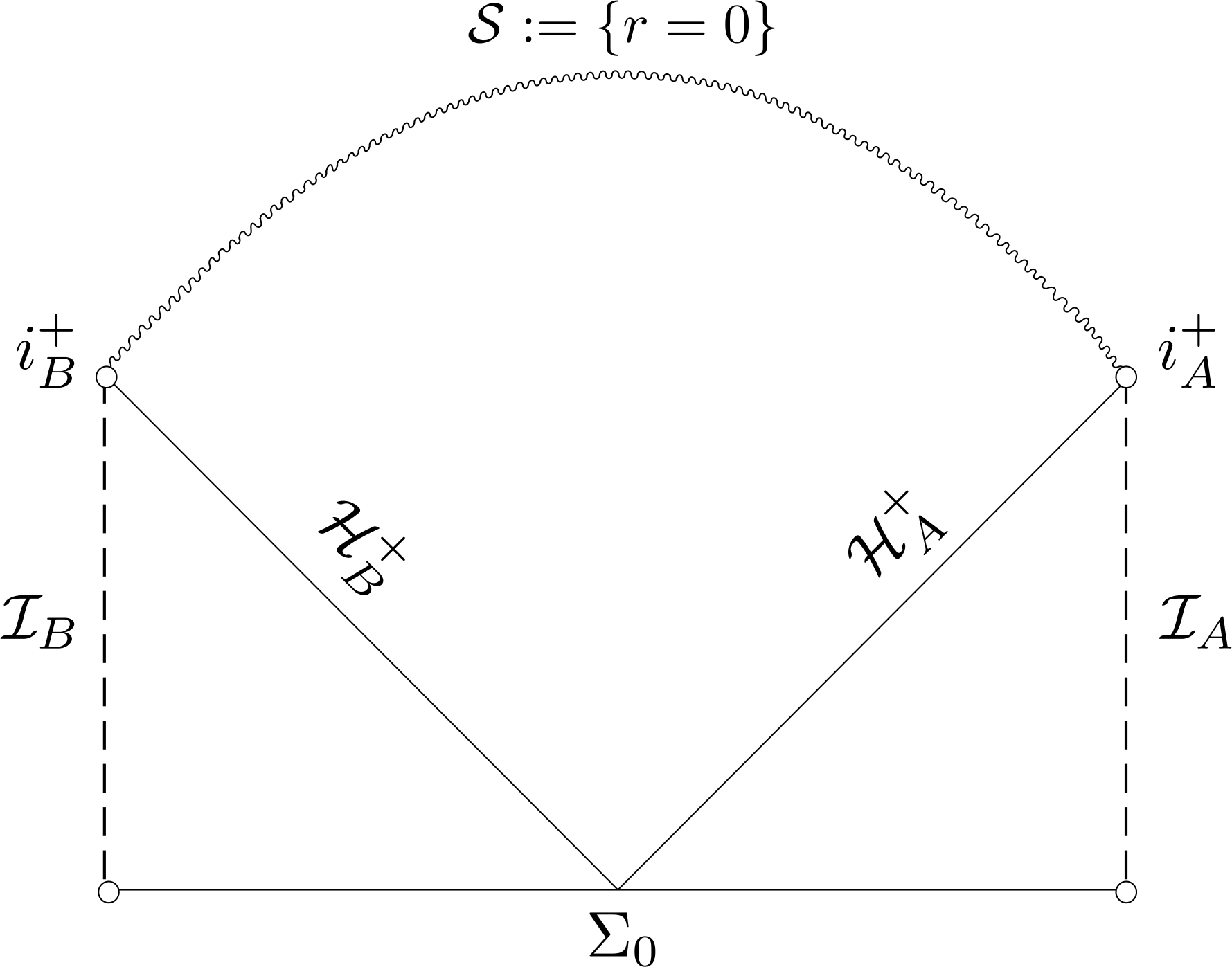
Figure 4: Penrose diagram of the asymptotically AdS two-ended black hole resolving Open Problem iv

1.7.3 Stability of $g_{\epsilon}$ with respect to non-homogeneous perturbations

After solving Open Problem iv and obtaining the metric $g_{\epsilon}$ covering both the black hole interior and exterior with AdS boundary conditions, a natural (and more demanding) problem to ask is the question of stability of $g_{\epsilon}$:

Open problem v.

Study the stability of $g_{\epsilon}$ against small, non static perturbations for the initial/boundary value problem.

Nonlinear stability problems with AdS boundary conditions are notoriously difficult, despite recent remarkable progress in spherical symmetry [50, 51, 52] (in the direction of instability, however). A more accessible question in the direction of Open Problem v is to first study only perturbations of the interior, for instance concrete data of the following form on the event horizon, with $f(v,\theta,\varphi)\rightarrow 0$ as $v\rightarrow+\infty$:

$$\phi_{|\mathcal{H}^{+}}(v,\theta,\varphi)=\epsilon+\epsilon^{2}\cdot f(v,\theta,\varphi).$$ (1.19)

In particular, in the case where $f(v,\theta,\varphi)=f(v)$ is spherically symmetric, it seems reasonable to expect that the quantitative methods of the present paper can be generalized to yield the stability of the interior region of $g_{\epsilon}$, at least if $f$ converges sufficiently fast to $0$. The non spherically-symmetric is expectedly more difficult, even though the recent breakthrough [24] proving the stability of Kasner for positive exponents (hence including the exponents that we obtain, see Section 1.5) could help in this direction, at least close enough to the singularity.

1.7.4 Rotating hairy black holes

A remarkable mathematical construction of a one-parameter family of rotating hairy black hole exteriors namely stationary, two-ended asymptotically flat solutions of the Einstein–Klein–Gordon system (1.1)-(1.4) (with $F\equiv 0$) that bifurcate off the Kerr metric has been carried out by Chodosh–Shlapentokh-Rothman [12]. Nevertheless, the interior of such hairy black holes has never been studied, and it is not known whether a Cauchy horizon exists as for the Kerr metric, or if it is replaced by a spacelike singularity as for $g_{\epsilon}$. This prompts the following problem:

Open problem vi.

Characterize the singularity inside the Chodosh–Shlapentokh-Rothman hairy black holes.

We plan to return to this problem in a future work.

1.7.5 Other matter models

Models where the singularity is conjectured to be Kasner-like

We already mentioned in detail in Section 1.5 the case of perturbations of Schwarzschild-(dS/AdS) and the main difference compared to the setting of Theorem I, together with the numerics [27] suggesting that the singularity is Kasner-like. This leads us to formulate the

Open problem vii.

Study spatially homogeneous perturbations of Schwarzschild-(dS/AdS) black holes.

As we explained in Section 1.6.2, the Einstein equations coupled with the SU(2)-Yang–Mills–Higgs equations also admit spatially homogeneous black hole interiors, and numerics [23], [22], [56] suggest a Kasner-like singularity:

Open problem viii.

Study spatially homogeneous solutions for the Einstein-SU(2)-Yang–Mills–Higgs equations.

Models where oscillations are conjectured

As we explained in Section 1.6.2, without a Higgs field, numerics suggest that the Einstein-SU(2)-Yang–Mills black holes admit a chaotic behavior in the interior [23], [7]. We are hopeful that the methods we developed in the present paper could also be adapted to address the following

Open problem ix.

Study spatially homogeneous solutions for the Einstein-SU(2)-Yang–Mills equations.

More closely related to our work is the generalization of Theorem I with the same data but for a more general model where the scalar field is allowed to be charged. In this case, the coupling with the Maxwell field is non trivial, and sourced by the charged scalar field. (This model was studied by the author [41], [42], [58], [59], [61] in a different setting where the scalar field decays to zero, instead of being a small constant (see Section 1.1)). Numerics [30] suggest very interesting dynamics in a certain parameter change for this system, in which oscillations precede the formation of a Kasner-like singularity with $p_{rad}<0$ (different from our scenario, recall Section 1.5) which is then inverted to a Kasner-like singularity with $p_{rad}>0$, a phenomenon the authors of [30] call “Kasner-inversion”.

Open problem x.

Study data as in Theorem I for the Einstein–Maxwell-charged–Klein–Gordon equations.

It would be extremely interesting to adapt the methods of the present paper to the setting of a charged scalar field, a problem we hope to return to in the future.

1.8 Strategy of the proof

1.8.1 Set-up of the problem and general description of the strategy

The data described in Theorem I give rise to a spatially homogeneous spacetime $\mathcal{M}_{\epsilon}=\mathbb{R}\times\mathbb{S}^{2}\times(0,r_{+}(M,e,\Lambda)]_{r}$, which we can describe as a superposition of $\mathbb{R}\times\mathbb{S}^{2}$ cylinders with variable area-radius $r$. The EMKG system (1.1)-(1.4) then reduces to a coupled system of nonlinear ODEs (see Section 2.4), that we analyze in physical space.

One of the main ideas behind the proof is to divide the spacetime into regions of the form $\{r_{inf}(\epsilon)<r<r_{\sup}(\epsilon)\}$ (or “epochs” since $r$ is a timelike coordinates in the interior). We will express these epochs using a time-coordinate $s$ (see (2.32) for a precise definition) which is monotonic with respect to $r$ (that is, $\frac{dr}{ds}<0$). $s\in(-\infty,s_{\infty}(\epsilon))$ can be thought of as a generalization of the standard $r^{*}\in\mathbb{R}$ coordinate on Reissner–Nordström. The data $\phi\equiv\epsilon\neq 0$ are posed on the event horizon $\mathcal{H}^{+}:=\{s=-\infty\}$ (Section 2.3) and we split the spacetime into (see Figure 1)

1. the red-shift region $\mathcal{R}:=\{-\infty<s\leq-\Delta(M,e,\Lambda,m^{2})\}$, for $\Delta(M,e,\Lambda,m^{2})>0$ sufficiently large.

2. the no-shift region $\mathcal{N}:=\{-\Delta<s\leq\Delta_{0}(\epsilon)\}$, $\Delta_{0}(\epsilon):=c(M,e,\Lambda,m^{2})\cdot\log(\epsilon^{-1})$ for $c(M,e,\Lambda,m^{2})>0$.

3. the early blue-shift region $\mathcal{EB}:=\{S^{\prime\prime}(M,e,\Lambda)<s\leq s_{lin}(\epsilon)\}$, $s_{lin}(\epsilon):=\frac{\log(\nu(M,e,\Lambda,m^{2})\cdot\epsilon^{-1})}{2|K_{-}|}$, for $\nu(M,e,\Lambda,m^{2})>0$ small enough, and $2K_{-}(M,e,\Lambda)$ is the surface gravity of the Reissner–Nordström-(dS/AdS) Cauchy horizon.

4. the late blue-shift region $\mathcal{LB}:=\{s_{lin}(\epsilon)<s\leq\epsilon^{-\frac{5}{4}}\}$.

5. the crushing region $\mathcal{C}:=\{\Delta_{\mathcal{C}}\cdot\epsilon^{-1}<s<s_{\infty}\}$, where $\Delta_{\mathcal{C}}(M,e,\Lambda,m^{2})>0$ and $s_{\infty}(\epsilon):=\frac{\epsilon^{-2}+O(\epsilon^{-1})}{4|K_{-}|\cdot b_{-}^{2}}<+\infty$.

6. The spacelike singularity $\mathcal{S}=\{r=0\}=\{s=s_{\infty}(\epsilon)\}$.

Remark 1.4.

Note that the regions $\mathcal{LB}$ and $\mathcal{C}$ both overlap with $\mathcal{N}$, overlap with each others, and that $\mathcal{EB}\subset\mathcal{N}$. Nevertheless, we have more precise estimates (using more sophisticated methods) on $\mathcal{EB}$ (respectively on $\mathcal{C}$) than on $\mathcal{N}$ (respectively on $\mathcal{LB}$) building on the less precise ones on the overlap between the regions.

Each region is characterized by a particular dynamical regime in which specific techniques apply, see below.

To estimate the EMKG system, we use a standard bootstrap method (which is crucial, in view of the nonlinearities) and prove weighted estimates (drastically different in each region) integrating along the time direction.

It is important to note that these physical space techniques have proven to be useful in many situations, even when the spacetime is not spatially-homogeneous or with many symmetries. In fact, we expect most of our estimates to generalize in some form to these more complex situations (see Section 1.7). We emphasize that our methods are entirely quantitative (and are inspired from those in [58] which deal with a spacetime with fewer symmetries, albeit with simpler dynamics) and that, even though $g_{\epsilon}$ are analytic spacetimes, we do not rely on analyticity at any stage.

Before turning to the nonlinear estimates, we will mention in Section 1.8.2 a preliminary linear result proven in [40] that will be useful in the early blue-shift region $\mathcal{EB}$ (where the dynamics is still mostly linear).

1.8.2 Preliminary estimates on the corresponding linearized solution

To capture the late time dynamics and the ultimate formation of the singularity (see Section 1.8.6), we require sharp estimates on the scalar field $\phi$. It is well-known that such sharp estimates cannot be obtained exclusively through physical spaces methods (see the discussion in [41]). Moreover, even for the linear wave equation $\Box_{g_{RN}}\phi_{\mathcal{L}}=m^{2}\phi_{\mathcal{L}}$ on a fixed Reissner–Nordström-(dS/AdS), the late time behavior depends on the parameters $(M,e,\Lambda,m^{2})$ (see [40]).

In our specific setting, the linearized version of $\phi$ from Theorem I corresponds to $\phi_{\mathcal{L}}^{(\epsilon)}=\epsilon\cdot\phi_{\mathcal{L}}^{(1)}$, where $\phi_{\mathcal{L}}^{(1)}$ is a solution of $\Box_{g_{RN}}\phi_{\mathcal{L}}^{(1)}=m^{2}\phi_{\mathcal{L}}^{(1)}$ with constant data $\phi_{\mathcal{L}}^{(1)}=1$ on $\mathcal{H}^{+}$. $\phi_{\mathcal{L}}^{(1)}$ solves a linear radial ODE in $r^{*}$ and

$$\phi_{\mathcal{L}}^{(1)}(r^{*})=A(M,e,\Lambda,m^{2})\cdot\tilde{v}_{1}(r^{*})+B(M,e,\Lambda,m^{2})\cdot\tilde{v}_{2}(r^{*}),\ \text{where }\tilde{v}_{1}(r^{*})\simeq 1,\ \tilde{v}_{2}(r^{*})\simeq r^{*}\text{ as }r^{*}\rightarrow+\infty.$$

One of the results of [40] is to show that for all sub-extremal parameters $(M,e,\Lambda)$ and almost every masses $m^{2}$:

$$B(M,e,\Lambda,m^{2})\neq 0.$$ (res)

a condition that we will refer to as a scattering resonance. When (res) is satisfied, $\phi_{\mathcal{L}}^{(1)}(r^{*})\approx r^{*}$ near the Reissner–Nordström-(dS/AdS) Cauchy horizon. The exceptional set $D(M,e,\Lambda)\subset\mathbb{R}$ of masses $m^{2}$ for which (res) is not true is called the set of non-resonant masses and it was shown in [40] that $0\in D(M,e,\Lambda)$, hence $D(M,e,\Lambda)$ is non-empty.

In the early regions (specifically $\mathcal{R}$, $\mathcal{N}$ and $\mathcal{EB}$), we will estimate the difference between the actual solution $\phi$ and the linearized $\phi_{\mathcal{L}}$ (see Section 1.8.3 for details) and show an estimate of the following form: for all $s\lesssim\log(\epsilon^{-1})$

$$|\phi(s)-\phi_{\mathcal{L}}(s)|\lesssim\epsilon^{3}.$$ (diff)

The bound (diff), however, is no longer true in future regions $\mathcal{LB}$ and $\mathcal{C}$ because the EMKG solution is dominated by the nonlinear regime at late time. The condition (res), in turn, is useless in $\mathcal{R}$ and $\mathcal{N}$, as it dictates the asymptotics of $\phi_{\mathcal{L}}$ close enough to the Cauchy horizon. But in $\mathcal{EB}$, two conditions are reunited to combine (diff) and (res): the EMKG system is still in the linear regime, and the metric is close (i.e. $s\sim\log(\epsilon^{-1})$ is large) to the Reissner–Nordström-(dS/AdS) Cauchy horizon (see Section 1.3 and Section 1.8.4). Thus, (diff) and (res) give sharp asymptotics in $\mathcal{EB}$:

$$|\phi(s)-B(M,e,\Lambda,m^{2})\cdot\epsilon|\lesssim\epsilon^{3}.$$ (1.20)

In the later regions $\mathcal{LB}$ and $\mathcal{C}$, we will build on (1.20) to construct the (genuinely nonlinear at this point) dynamics of $\phi$ which critically affects the behavior of the metric $g_{\epsilon}$, especially the spacelike singularity formation. In particular, the Kasner exponents depend (Section 1.5) on what we call the resonance parameter $b_{-}\in\mathbb{R}$

$$b_{-}(M,e,\Lambda,m^{2}):=\frac{B(M,e,\Lambda,m^{2})}{2|K_{-}|(M,e,\Lambda)}\neq 0, b_{-}$$ ()

where $2K_{-}(M,e,\Lambda)<0$ is the surface gravity of the unperturbed Cauchy horizon (recall $b_{-}$ is used in Theorem I).

1.8.3 The red-shift region $\mathcal{R}$ and the no-shift region $\mathcal{N}$: Cauchy stability regime

Recall the definition of the regions $\mathcal{R}$ and $\mathcal{N}$ from Section 1.8.1. These regions are easier for the following reasons:

1. The range of $s$ in $\mathcal{R}$ is infinite, but the spacetime volume is small. Moreover, one can exploit the classical red-shift estimates for the wave equation (and, by extension, for the EMKG system).

2. The range of $s$ in $\mathcal{N}$ is finite, but large (i.e. $O(\log(\epsilon^{-1}))$). Nevertheless, the range of $s$ to the future of $\mathcal{N}$ is $O(\epsilon^{-2})$ and $\log(\epsilon^{-1})\ll\epsilon^{-2}$ so $\mathcal{N}$ is considered to be “a small region”, compared to the rest of the spacetime.

In particular, in these two regions, the principle of Cauchy stability, which roughly states that $\epsilon$ perturbations in the data give rise to $O(\epsilon^{2})$ perturbations for the solutions of quadratic nonlinear PDEs, prevails.

Concretely, for all $s\in\mathcal{R}:=\{-\infty<s\leq-\Delta\}$ for $\Delta(M,e,\Lambda,m^{2})$ large, we show the schematic estimates:

$$|g(s)-g_{RN}(s)|\lesssim\epsilon^{2}\cdot e^{2K_{+}(M,e,\Lambda)s}\ll\epsilon^{2},$$ (R1)

$$|\frac{dg}{ds}(s)-\frac{dg_{RN}}{ds}(s)|\lesssim\epsilon^{2}\cdot e^{2K_{+}(M,e,\Lambda)s}\ll\epsilon^{2},$$ (R2)

$$|\kappa^{-1}(s)-1|\lesssim\epsilon^{2}\cdot e^{2K_{+}(M,e,\Lambda)s}\ll\epsilon^{2},$$ (R3)

$$|\phi(s)-\phi_{\mathcal{L}}(s)|\lesssim\epsilon^{3}\cdot e^{2K_{+}(M,e,\Lambda)s}\ll\epsilon^{3},$$ (R4)

where $\kappa^{-1}:=\frac{-\frac{dr}{ds}}{\Omega^{2}}$ ($\kappa^{-1}=1$ on Reissner–Nordström-(dS/AdS)) and $2K_{+}(M,e,\Lambda)>0$ is the surface gravity of the event horizon. The factor $e^{2K_{+}s}$ is the sign of red-shift, and requiring $\Delta$ to be large gives $e^{2K_{+}s}\ll 1$ for $s<-\Delta$.

In the no-shift region $\mathcal{N}$ $:=\{-\Delta<s\leq c(M,e,\Lambda,m^{2})\cdot\log(\epsilon^{-1})\}$, we use Gronwall estimates: for all $s\in\mathcal{N}$

$$|g(s)-g_{RN}(s)|\lesssim C^{s}\cdot\epsilon^{2}\lesssim\epsilon,$$ (N1)

$$|\frac{dg}{ds}(s)-\frac{dg_{RN}}{ds}(s)|\lesssim C^{s}\cdot\epsilon^{2}\lesssim\epsilon,$$ (N2)

$$|\phi(s)-\phi_{\mathcal{L}}(s)|\lesssim C^{s}\cdot\epsilon^{3}\lesssim\epsilon^{2},$$ (N3)

where $C(M,e,\Lambda,m^{2}):=e^{c^{-1}}$. In the above estimates, the term $C^{s}\lesssim\epsilon^{-1}$ is indeed the sign of the loss incurred by the use of Gronwall. To avoid this loss, we will only use the above for $s\leq S^{\prime\prime}(M,e,\Lambda,m^{2})$ where $S^{\prime\prime}(M,e,\Lambda,m^{2})>0$ is a large constant but independent of $\epsilon$ (recall that the past boundary of the next region $\mathcal{EB}$ is at $s=S^{\prime\prime}(M,e,\Lambda,m^{2})$).

Completing these steps provides estimates on the difference between the dynamical metric $g_{\epsilon}$ and its unperturbed background $g_{RN}$ (recall $g_{\epsilon}=g_{RN}$ on the data, see Theorem I) in the strong $C^{1}$ norm, up to $\mathcal{EB}$. This explains the stability of the Cauchy horizon claimed in Theorem I; in particular, for any constant $\Gamma>0$, $g_{\epsilon}$ is uniformly close to $g_{RN}$ for $s<\Gamma$, for $|\epsilon|$ small enough (we will extend these estimates up to $s\ll\epsilon^{-1}$, but they fail for $s\simeq\epsilon^{-2}$).

Remark 1.5.

Going forward, we will actually not directly need $g-g_{RN}$ estimates in $\mathcal{C}$ to prove the formation of a spacelike singularity: nevertheless, we will need (1.20), for which we do need $g-g_{RN}$ to be small in the past of $\mathcal{EB}$. Thus, there is no obvious way to avoid difference estimates on the metric to show that the singularity is spacelike.

1.8.4 The early blue-shift region $\mathcal{EB}$: Reissner–Nordström-(dS/AdS) stability in strong norms

In the early blue-shift region $\mathcal{EB}=\{S^{\prime\prime}(M,e,\Lambda)<s\leq s_{lin}(\epsilon)\}\subset\mathcal{N}$, Cauchy stability, as defined earlier, does not give sharp bounds, so we look for different paths towards improvement. We will exploit the so-called blue-shift effect, which traditionally occurs at the Cauchy horizon of Reissner–Nordström-(dS/AdS) for large $s$. To understand its manifestation, recall the lapse $\Omega^{2}$ from (1.15): the typical estimate we obtain in this region is

$$\bigl{|}\frac{d}{ds}\log(\Omega^{2})(s)-2K_{-}(M,e,\Lambda)\bigr{|}\lesssim e^{2K_{-}s}\ll\frac{|K_{-}|}{100},$$

where $2K_{-}(M,e,\Lambda)<0$ is the surface gravity of the Reissner–Nordström-(dS/AdS) Cauchy horizon and $S^{\prime\prime}(M,e,\Lambda)>0$ is chosen to be sufficiently large so that the last inequality holds. This enforces a behavior of the following form:

$$\Omega^{2}(s)\approx e^{2K_{-}s},$$ (blue-shift)

an estimate which is also valid on Reissner–Nordström-(dS/AdS), close enough to the Cauchy horizon. Since $e^{2K_{-}S^{\prime\prime}}\ll 1$, $\Omega^{2}$ is small, which is helpful to close difference estimates with an (inconsequential) logarithmic loss (compare with the much worse estimates from (N1), (N2), (N3)), i.e. for all $s\in\mathcal{EB}$:

$$|g(s)-g_{RN}(s)|\lesssim\epsilon^{2}\cdot s\lesssim\epsilon^{2}\cdot\log(\epsilon^{-1}),$$ (EB1)

$$|\frac{dg}{ds}(s)-\frac{dg_{RN}}{ds}(s)|\lesssim\epsilon^{2}\cdot s\lesssim\epsilon^{2}\cdot\log(\epsilon^{-1}),$$ (EB2)

$$|\phi(s)-\phi_{\mathcal{L}}(s)|\lesssim\epsilon^{3}\cdot s\lesssim\epsilon^{3}\cdot\log(\epsilon^{-1}).$$ (EB4)

The analogue of (R3) is different; using (blue-shift) and the Raychaudhuri equation (2.25), we get for all $s\in\mathcal{EB}$

$$|\kappa^{-1}(s)-1|\lesssim\frac{\epsilon^{2}}{\Omega^{2}(s)}\approx\epsilon^{2}\cdot e^{2|K_{-}|s}<0.1,$$ (1.21)

and the future boundary $\{s=s_{lin}\simeq\log(\epsilon^{-1})\}$ of $\mathcal{EB}$ is chosen so that the RHS of (1.21) is $<0.1$, hence $\Omega^{2}(s_{lin})\approx\epsilon^{2}$.

Remark 1.6.

Going forward, we note that in $\mathcal{N}-\mathcal{EB}$ (and also in $\mathcal{LB}$), $\kappa^{-1}$ becomes larger and larger, a sign of the classical blue-shift instability (see Section 1.8.5). This growth is an obstruction to showing sharp difference bounds, which explains why we isolate $\mathcal{EB}$ inside $\mathcal{N}$, and also prompts the use of a new strategy in the next region $\mathcal{LB}$.

1.8.5 The late blue-shift region $\mathcal{LB}$: Reissner–Nordström-(dS/AdS) stability in weak norms

Unlike its predecessors, the late blue-shift region $\mathcal{LB}:=\{s_{lin}(\epsilon)<s\leq\epsilon^{-\frac{5}{4}}\}$ has a large $s$-range of order $O(\epsilon^{-\frac{5}{4}})$ and Cauchy stability utterly fails, two facts that render the estimates noticeably more delicate. The failure of Reissner–Nordström-(dS/AdS) stability in strong $C^{1}$ norm can be expressed for instance in the following estimate:

$$\kappa^{-1}(s)\approx\epsilon^{2}\cdot e^{2|K_{-}|s}\ \Rightarrow\ \kappa^{-1}(\epsilon^{-\frac{5}{4}})\approx\epsilon^{2}\cdot e^{O(\epsilon^{-\frac{5}{4}})}\gg 1,$$ (1.22)

and a similar estimate holds for the Hawking mass $\rho$, which becomes large. Relatedly, in the non-hairy case when $\phi$ tends to $0$ (discussed in Section 1.1), it is known that mass inflation is caused by the blue-shift effect (see [61]); we see some reminiscence of this phenomenon in the hairy case as reflected by (1.22) and the related estimate on $\rho$.

As should be clear, difference estimates (as we had earlier) cannot be proved in $\mathcal{LB}$. However, we still obtain some form of weak Reissner–Nordström-(dS/AdS) stability in the $C^{0}$ norm: recalling the definition of $r$ from (1.15)

$$|r(s)-r_{-}(M,e,\Lambda)|\lesssim\epsilon^{2}\cdot s\lesssim\epsilon^{\frac{3}{4}}\leq\frac{r_{-}(M,e,\Lambda)}{100},$$ (LB1)

$$\Omega^{2}(s)\approx e^{2K_{-}s},$$ (LB1)

$$|\phi(s)-A(M,e,\Lambda,m^{2})\cdot\epsilon-B(M,e,\Lambda,m^{2})\cdot\epsilon\cdot s|\lesssim\epsilon^{2}\cdot s^{2}\lesssim\epsilon^{-\frac{1}{2}}.$$ (LB3)

(LB3) is a particularly bad zeroth order estimate. At the first order, however, we get a much sharper control:

$$\bigl{|}r^{2}(s)\cdot\frac{d\phi}{ds}(s)-r_{-}^{2}\cdot B(M,e,\Lambda,m^{2})\cdot\epsilon\bigr{|}\lesssim\epsilon^{3}. \dot{\phi}$$ ()

Going forward, estimate ($\dot{\phi}$) will be crucial in the spacelike singularity formation in $\mathcal{C}$. Obtaining ($\dot{\phi}$) was in truth the main motivation behind all the estimates that we wrote earlier, including the metric difference estimates.

Finally, we prove the following estimate on $\frac{dr}{ds}:=\dot{r}$, which will be important in the crushing region $\mathcal{C}$:

$$-\dot{r}(s)\simeq\frac{\epsilon^{2}}{r(s)}. \dot{r}$$ ()

Note that, near the future boundary of $\mathcal{LB}$, ($\dot{r}$) differs drastically from the Reissner–Nordström-(dS/AdS) bounds $-\dot{r}_{RN}(s)\approx e^{2K_{-}s}$. This is yet another sign of the nonlinear violent collapse, see Section 1.8.6 below.

1.8.6 The crushing region $\mathcal{C}$: nonlinear regime and spacelike singularity formation

Recall the estimates obtained in $\mathcal{LB}$ are far from sharp in the region $\epsilon^{-1}\ll s\lesssim\epsilon^{-\frac{5}{4}}$; for technical reasons, we define $\mathcal{C}:=\{\Delta_{\mathcal{C}}\cdot\epsilon^{-1}<s<s_{\infty}\}$ to overlap substantially with $\mathcal{LB}$, so that estimates on the past of $\mathcal{C}$ are still usable.

In contrast to the bounds obtained in past regions, that were inspired from [58] (in the context where the Cauchy horizon is stable), the region $\mathcal{C}$ has a new behavior. A nonlinear bifurcation occurs, driving the dynamical system away from Reissner–Nordström-(dS/AdS) and towards a Kasner metric (Section 1.5). The key ingredient is an estimate on the null lapse $\Omega^{2}$ (see (1.15)) which ultimately makes the spacetime volume of $\mathcal{C}$ much smaller than expected (see heuristics in Section 1.4): we prove that $\Omega^{2}$ tends to $0$ as a large $r$ power. Specifically, for all $s\in\mathcal{C}$:

$$\Omega^{2}(s)\simeq\epsilon^{2}\cdot(\frac{r(s)}{r_{-}})^{b_{-}^{-2}\cdot\epsilon^{-2}}.$$ (C1)

By (C1), we can schematically neglect the terms proportional to $\Omega^{2}$ in the EMKG system of ODEs (Section 2.4):

$$\frac{d^{2}\log(r\Omega^{2})}{ds^{2}}=-2|\frac{d\phi}{ds}|^{2}+\frac{\Omega^{2}}{r^{2}}(1-\frac{3e^{2}}{r^{2}}+m^{2}r^{2}|\phi|^{2}+\Lambda r^{2})\approx-2|\frac{d\phi}{ds}|^{2},$$ (1.23)

$$\frac{d}{ds}(-r\dot{r})=\Omega^{2}\cdot(1-\frac{e^{2}}{r^{2}})-r^{2}\Omega^{2}(\Lambda+m^{2}|\phi|^{2})\approx 0,$$

$$\frac{d}{ds}(r^{2}\dot{\phi})=-m^{2}r^{2}\Omega^{2}\phi\approx 0.$$

The three above equations are of course mere heuristics we give to explain the proof: for details, see Section 4.5. Once these heuristics have been made rigorous, they show that ($\dot{r}$) and ($\dot{\phi}$) are still valid in $\mathcal{C}$. To prove (C1) (which is as of now just a bootstrap assumption), we plug ($\dot{r}$) and ($\dot{\phi}$) into (1.23) and integrate: schematically

$$\frac{d^{2}\log(r\Omega^{2})}{ds^{2}}\approx-2|\frac{d\phi}{ds}|^{2}\approx-\frac{\epsilon^{2}}{r^{4}}\approx\frac{\dot{r}}{r^{3}}\ \Rightarrow\ \frac{d\log(r\Omega^{2})}{ds}\approx-\frac{1}{r^{2}}\approx\frac{\epsilon^{-2}\cdot\dot{r}}{r}\ \Rightarrow\ \log(r\Omega^{2})\approx\log(r^{\epsilon^{-2}}).$$

Now that we have explained the main elements behind the estimates, we make important qualitative comments:

1. $\mathcal{C}$ is the only region where $r$ is not bounded away from zero. While the $r$-dependency of ($\dot{r}$) and ($\dot{\phi}$) was inconsequential in $\mathcal{LB}$, it becomes crucial in $\mathcal{C}$, as it dictates the behavior of all the other quantities as $r\rightarrow 0$.

2. $\dot{\phi}$ and $\dot{r}$ blow-up with the same $r$ power as on Schwarzschild at $r=0$, but the pre-factor is different, which impacts dramatically the dynamics, and is responsible for violent nonlinear collapse (see Section 1.4).

3. The drastic difference between ($\dot{r}$) and ($\dot{\phi}$) and their Schwarzschild analogue can be interpreted as a consequence of the almost stability of the Reissner–Nordström-(dS/AdS) Cauchy horizon and its associated blue-shift effect, which provides “non-typical” initial data on $\{s=\Delta_{\mathcal{C}}\cdot\epsilon^{-1}\}$ the past boundary of $\mathcal{C}$.

4. The dynamics are governed by the nonlinearity $-2|\frac{d\phi}{ds}|^{2}$ in the Gauss equation (1.23). This term is responsible for a monotonicity-driven collapse, which is reminiscent of the stable blow-up dynamics near Kasner in [24].

5. To show (C1), we needed sharp estimates on $\phi$ already in the past, given by ($\dot{\phi}$) (showing that $\phi$ differs from $\phi_{\mathcal{L}}$ in $\mathcal{LB}$), itself following from (EB4), an estimate that uses the presence of a linear resonance i.e. (res).

All the power law bounds e.g. (1.7) follow directly from (C1); they are more compelling than (C1) as they do not depend on the choice of the coordinate $s$: the Hawking mass and the Kretschmann scalar are geometric quantities.

As a consequence of ($\dot{r}$) (still valid in $\mathcal{C}$), we show that there exists $s_{\infty}<+\infty$ with $s_{\infty}(\epsilon)\simeq\epsilon^{-2}$ such that

$$\lim_{s\rightarrow s_{\infty}}r(s)=0,$$

therefore $\mathcal{S}:=\{r=0\}$ is indeed a spacelike singularity, since $s$ is finite at $\mathcal{S}$ and $g=-\Omega^{2}(-dt^{2}+ds^{2})+d\sigma_{\mathbb{S}^{2}}$.

Lastly, we recall that (C1) translates into a Kasner behavior as explained in Section 1.5, see also Theorem 3.3.

1.9 Acknowledgments

I warmly thank Mihalis Dafermos for mentioning this problem to me, for his interest in its resolution, and many helpful comments on the manuscript. I am grateful to Christoph Kehle and Yakov Shlapentokh–Rothman for interesting discussions and for explaining certain aspects of their work, and to Hans Ringström for kindly answering my questions related to cosmology. I would like to warmly thank Jorge Santos for enlightening discussions about his work, and AdS-CFT in general. I am grateful to Jonathan Luk and Harvey Reall for useful comments on the manuscript.

1.10 Outline of the paper

In Section 2, we introduce the Reissner-Nordström-(dS/AdS) metric, the class of spatially-homogeneous spacetimes that we consider, specify the data of Theorem I, and the reduction of the Einstein equations as a system of nonlinear ODEs. We also mention a result on the linearized dynamics from [40] that we will be needing.

In Section 3, we provide a precise statement of the results that were condensed in Theorem I: Theorem 3.1 (main theorem), Theorem 3.2 (convergence to Reissner-Nordström), Theorem 3.3 (Kasner behavior).

In Section 4, we prove Theorem 3.1 and provide many useful quantitative estimates.

Section 5 is a short proof of Theorem 3.2, entirely based on the quantitative estimates of Section 4.

In Section 6, we prove Theorem 3.3, mostly based again on the quantitative estimates of Section 4 and also using certain renormalization procedures and convergence estimates.

2 Preliminaries

2.1 The Reissner-Nordström-(dS/AdS) interior metric

Before defining the Reissner-Nordström-(dS/AdS) metric, we introduce the set of sub-extremal parameters $(M,e,\Lambda)\in\mathbb{R}_{+}^{*}\times\mathbb{R}^{2}$ defined as $\mathcal{P}_{se}:=\mathcal{P}_{se}^{\Lambda>0}\cup\mathcal{P}_{se}^{\Lambda\leq 0}$ where $\mathcal{P}_{se}^{\Lambda\leq 0}$ consists of all $(M,e,\Lambda)\in\mathbb{R}_{+}^{*}\times\mathbb{R}\times\mathbb{R}_{-}$ such that the polynomial $X^{2}-2MX+e^{2}-\frac{\Lambda X^{4}}{3}$ has two positive simple roots $r_{-}<r_{+}$ and $\mathcal{P}_{se}^{\Lambda>0}$ of of all $(M,e,\Lambda)\in\mathbb{R}_{+}^{*}\times\mathbb{R}\times\mathbb{R}_{+}^{*}$ such that the polynomial $X^{2}-2MX+e^{2}-\frac{\Lambda X^{4}}{3}$ has three positive simple roots $r_{-}<r_{+}<r_{c}$.

Let $(g_{RN},F_{RN})$ be an electro-vacuum solution of (1.1)-(1.4) i.e. a solution with $\phi\equiv 0$, given by

$$g_{RN}=-(1-\frac{2M}{r_{RN}}+\frac{e^{2}}{r^{2}_{RN}}-\frac{\Lambda r^{2}_{RN}}{3})dt^{2}+(1-\frac{2M}{r_{RN}}+\frac{e^{2}}{r^{2}_{RN}}-\frac{\Lambda r^{2}_{RN}}{3})^{-1}dr^{2}_{RN}+r^{2}_{RN}[d\theta^{2}+\sin(\theta)^{2}d\varphi^{2}], g_{RN}$$ ()

$$F_{RN}=\frac{e}{r^{2}}dt\wedge dr, F_{RN}$$ ()

in the coordinate range $t\in\mathbb{R}$, $r_{RN}\in[r_{-}(M,e,\Lambda),r_{+}(M,e,\Lambda)]$ and where $(M,e,\Lambda)\in\mathcal{P}_{se}$ and $r_{\pm}(M,e,\Lambda)>0$ are the roots of the polynomial $X^{2}-2MX+e^{2}-\frac{\Lambda X^{4}}{3}$. For $\Lambda=0$ (resp. $\Lambda>0$, resp. $\Lambda<0$), the metric given by ($g_{RN}$) is called the sub-extremal Reissner-Nordström (resp. de Sitter, resp. Anti-de Sitter) interior metric. Define:

$$\frac{dr^{*}}{dr_{RN}}:=\frac{1}{\Omega^{2}_{RN}(r_{RN})},\hskip 5.69054pt\Omega^{2}_{RN}(r_{RN}):=-(1-\frac{2M}{r_{RN}}+\frac{e^{2}}{r^{2}_{RN}}-\frac{\Lambda r_{RN}^{2}}{3}),$$ (2.1)

$$u:=\frac{r^{*}-t}{2},\hskip 5.69054ptv:=\frac{r^{*}+t}{2},$$ (2.2)

in the range $u\in\bar{\mathbb{R}}$, $v\in\bar{\mathbb{R}}$, $r^{*}\in\bar{\mathbb{R}}$. We attach the following so-called event horizons to the space-time:

$$\mathcal{H}_{L}^{+}:=\{v=-\infty\},\hskip 5.69054pt\mathcal{H}_{R}^{+}:=\{u=-\infty\},\hskip 5.69054pt\mathcal{H}^{+}:=\mathcal{H}_{L}^{+}\cup\mathcal{H}_{R}^{+}=\{r^{*}=-\infty\}.$$ (2.3)

Note that in the $(u,v,\theta,\psi)$ coordinate system, ($g_{RN}$) takes the form

$$g_{RN}=-\Omega^{2}_{RN}dudv+r^{2}_{RN}[d\theta^{2}+\sin(\theta)^{2}d\varphi^{2}].$$

It is a classical computation (see e.g. [58]) that there exists a constant $\alpha_{+}(M,e,\Lambda)>0$ such that as $r^{*}\rightarrow-\infty$

$$\Omega^{2}_{RN}(r^{*})\sim\alpha_{+}\cdot e^{2K_{+}(M,e,\Lambda)\cdot r^{*}}=\alpha_{+}\cdot e^{2K_{+}(M,e,\Lambda)\cdot(u+v)},$$ (2.4)

where $2K_{+}(M,e,\Lambda)>0$ is the so-called surface of the gravity of the event horizon and we also define more generally

$$2K_{\pm}(M,e,\Lambda)=\frac{2}{r_{\pm}(M,e,\Lambda)}(M-\frac{e^{2}}{r_{\pm}(M,e,\Lambda)}-\frac{\Lambda r_{\pm}^{3}(M,e,\Lambda)}{3}), K_{\pm}$$ ()

noting that the so-called surface gravity of the Cauchy horizon $2K_{-}(M,e,\Lambda)<0$ is strictly negative.

Lastly, we also define “regular coordinates” $(U,V)$ as follows

$$\frac{dU}{du}=e^{2K_{+}u},\hskip 5.69054ptU(u=-\infty)=0.$$ (2.5)

$$\frac{dV}{dv}=e^{2K_{+}v},\hskip 5.69054ptV(v=-\infty)=0.$$ (2.6)

2.2 2-surface symmetric metrics and (1.1)–(1.4) in double null coordinates

We consider a 2-surface symmetric Lorentzian manifold $(M,g)$ taking the following form in null coordinates $(u,v)$:

$$g=g_{\mathcal{Q}}+r^{2}d\Sigma_{k}=-4\Omega^{2}dudv+r^{2}d\Sigma_{k},$$ (2.7)

$$\begin{split}d\Sigma_{1}=d\theta^{2}+\sin^{2}(\theta)d\varphi^{2},\hskip 14.22636ptd\Sigma_{-1}=d\theta^{2}+\sinh^{2}(\theta)d\varphi^{2},\hskip 14.22636ptd\Sigma_{0}=dx^{2}+dy^{2}.\end{split}$$ (2.8)

where $d\Sigma_{k}$ is the metric of constant curvature $k\in\{-1,0,1\}$ (respectively on $\mathbb{H}^{2}$, $\mathbb{T}^{2}$ or $\mathbb{S}^{2}$) and we call $r$ the area-radius. We also define the Hawking mass by the formula:

$$\rho:=\frac{r}{2}(1-g_{\mathcal{Q}}(\nabla r,\nabla r)).$$

In the presence of the Maxwell field ($F_{RN}$), we define the Vaidya mass $\varpi$ and the constant-$r$ surface gravity $2K$:

$$\varpi:=\rho+\frac{e^{2}}{2r}-\frac{\Lambda r^{3}}{6},\hskip 5.69054pt2K=\frac{2}{r^{2}}(\varpi-\frac{e^{2}}{r}-\frac{\Lambda r^{3}}{3}).$$ (2.9)

An elementary computation shows that (note that the normalization of $\Omega^{2}$ differs from [58] by a factor $4$)

$$\frac{-\partial_{u}r\partial_{v}r}{\Omega^{2}}=1-\frac{2\varpi}{r}+\frac{e^{2}}{r^{2}}-\frac{\Lambda r^{2}}{3}.$$ (2.10)

Let $\phi$ a real-valued spherically symmetric scalar field on $(M,g)$ such that $(g,F_{RN},\phi)$ is a solution of (1.1)–(1.4). Then, $(r,\Omega^{2},\phi)$ satisfy the following system of PDE’s in any double-null $(u,v)$ coordinates:

$$\partial_{u}\partial_{v}r=\frac{-\Omega^{2}}{r}-\frac{\partial_{u}r\partial_{v}r}{r}+\frac{\Omega^{2}}{r^{3}}e^{2}+r\Omega^{2}(\Lambda+m^{2}|\phi|^{2})=-\Omega^{2}\cdot 2K+r\Omega^{2}(\Lambda+m^{2}|\phi|^{2}),$$ (2.11)

$$\partial_{u}\partial_{v}\log(\Omega^{2})=-2\partial_{u}\phi\partial_{v}\phi+\frac{2\Omega^{2}}{r^{2}}+\frac{2\partial_{u}r\partial_{v}r}{r^{2}}-\frac{4\Omega^{2}}{r^{4}}e^{2},$$ (2.12)

$$\partial_{u}(\frac{\partial_{u}r}{\Omega^{2}})=\frac{-r}{\Omega^{2}}|\partial_{u}\color[rgb]{0,0,0}\phi|^{2},$$ (2.13)

$$\partial_{v}(\frac{\partial_{v}r}{\Omega^{2}})=\frac{-r}{\Omega^{2}}|\partial_{v}\color[rgb]{0,0,0}\phi|^{2},$$ (2.14)

$$\partial_{u}\partial_{v}\phi=-\frac{\partial_{v}r\partial_{u}\phi}{r}-\frac{\partial_{u}r\partial_{v}\phi}{r}-m^{2}\Omega^{2}\phi.$$ (2.15)

2.3 Set-up of the initial data

We pose characteristic data for (2.11)–(2.15) on two affine-complete null hypersurfaces $\mathcal{H}^{+}_{L}:=\{v=-\infty,u\in\mathbb{R}\}$ and $\mathcal{H}^{+}_{R}:=\{u=-\infty,v\in\mathbb{R}\}$ intersecting at a sphere, where $(u,v)$ are renormalized by the following gauge conditions:

$$\frac{-\partial_{u}r}{\Omega^{2}}_{|\mathcal{H}^{+}_{R}}(v)=1,\hskip 5.69054pt\frac{-\partial_{v}r}{\Omega^{2}}_{|\mathcal{H}^{+}_{L}}(u)=1.$$ (2.16)

The data we consider consist of sub-extremal Reissner-Nordström (dS/AdS) data for $(r,\Omega^{2})$ and a constant function $\phi$ on $\mathcal{H}^{+}_{L}\cup\mathcal{H}^{+}_{R}$, more precisely for some $(e,M,\Lambda)\in\mathcal{P}_{se}$ and some $\epsilon\neq 0$ (recall the definition of $\alpha_{+}>0$ from (2.4)):

$$r_{|\mathcal{H}^{+}_{L}\cup\mathcal{H}^{+}_{R}}\equiv r_{+}(M,e,\Lambda), r$$ (-data)

$$\left(\frac{\Omega^{2}}{e^{2K_{+}\cdot(u+v)}}\right)_{|\mathcal{H}^{+}_{L}\cup\mathcal{H}^{+}_{R}}\equiv\alpha_{+}(M,e,\Lambda), \Omega^{2}$$ (-data)

$$\phi_{|\mathcal{H}^{+}_{L}\cup\mathcal{H}^{+}_{R}}\equiv\epsilon. \phi$$ (-data)

One can check that such data are compatible with the (null) constraints imposed on $\mathcal{H}^{+}_{L}\cup\mathcal{H}^{+}_{R}$ by (2.11)–(2.15). Recalling that $(u,v)$ are defined by (2.16), we define coordinates $U$ and $V$ by the formulae (2.5), (2.6), thus $\mathcal{H}^{+}_{L}:=\{V=0,u\in\mathbb{R}\}$ and $\mathcal{H}^{+}_{R}:=\{U=0,v\in\mathbb{R}\}$ . Then by (2.15) we have the following identities

$$(\partial_{v}\partial_{U}\phi)_{|\mathcal{H}^{+}_{R}}=-m^{2}\cdot\alpha_{+}(M,e,\Lambda)\cdot e^{2K_{+}(M,e,\Lambda)v}\epsilon,$$

$$(\partial_{u}\partial_{V}\phi)_{|\mathcal{H}^{+}_{L}}=-m^{2}\cdot\alpha_{+}(M,e,\Lambda)\cdot e^{2K_{+}(M,e,\Lambda)u}\epsilon.$$

Integrating using the boundary condition $\partial_{U}\phi(0,0)=\partial_{V}\phi(0,0)=0$ at the bifurcation sphere $\{U=V=0\}$ gives

$$(\partial_{U}\phi)_{|\mathcal{H}^{+}_{R}}(v)=-m^{2}\cdot\beta_{+}(M,e,\Lambda)\cdot e^{2K_{+}(M,e,\Lambda)v}\cdot\epsilon,$$ (2.17)

$$(\partial_{V}\phi)_{|\mathcal{H}^{+}_{L}}(u)=-m^{2}\cdot\beta_{+}(M,e,\Lambda)\cdot e^{2K_{+}(M,e,\Lambda)u}\cdot\epsilon.$$ (2.18)

where $\beta_{+}(M,e,\Lambda):=\frac{\alpha_{+}(M,e,\Lambda)}{2K_{+}(M,e,\Lambda)}>0$. In particular, note that $(\partial_{u}\phi)_{|\mathcal{H}^{+}_{R}}\equiv 0$ and $(\partial_{v}\phi)_{|\mathcal{H}^{+}_{L}}\equiv 0$.

2.4 System of ODEs for static solutions and initial data

Let $t:=v-u$ and $s:=v+u$ where $(u,v)$ are given by (2.16). For the data of Section 2.3, it is clear that $\partial_{t}r$, $\partial_{t}\log(\Omega^{2})$, $\partial_{t}\phi=0$ on the initial surfaces $\mathcal{H}^{+}_{L}\cup\mathcal{H}^{+}_{R}$ (recall the discussion in Section 2.3). Therefore, $\partial_{t}r$, $\partial_{t}\log(\Omega^{2})$, $\partial_{t}\phi=0$ for solutions $(r,\Omega^{2},\phi)$ of the 2D PDE (2.11)–(2.15) with the data of Section 2.3. In view of the identities

$$\partial_{u}=\partial_{s}-\partial_{t},\hskip 5.69054pt\partial_{u}=\partial_{s}+\partial_{t},$$

it is clear for that all $f\in\{r(s),\Omega^{2}(s),\phi(s)\}$, $\partial_{u}f=\partial_{v}f=\frac{df}{ds}$. In the $(t,s,\theta,\varphi)$ coordinate system, (2.7) becomes

$$g=\Omega^{2}(s)(-ds^{2}+dt^{2})+r^{2}(s)d\sigma_{\mathbb{S}^{2}}.$$ (2.19)

Using the notation $\frac{df}{ds}=\dot{f}$, the Einstein–(Maxwell)– Klein-Gordon equations (2.11)–(2.15) can be written as

$$\ddot{r}=\frac{-\Omega^{2}}{r}-\frac{\dot{r}^{2}}{r}+\frac{\Omega^{2}}{r^{3}}e^{2}+r\Omega^{2}(\Lambda+m^{2}|\phi|^{2}),$$ (2.20)

which is also equivalent to

$$\frac{d}{ds}(-r\dot{r})=\Omega^{2}\cdot(1-\frac{e^{2}}{r^{2}})-r^{2}\Omega^{2}(\Lambda+m^{2}|\phi|^{2}),$$ (2.21)

or

$$\frac{d}{ds}(\frac{-\dot{r}}{r})=2(\frac{-\dot{r}}{r})^{2}+\Omega^{2}\cdot(\frac{1}{r^{2}}-\frac{e^{2}}{r^{4}})-\Omega^{2}(\Lambda+m^{2}|\phi|^{2})$$ (2.22)

$$\frac{d^{2}\log(\Omega^{2})}{ds^{2}}=-2|\dot{\phi}|^{2}+\frac{2\Omega^{2}}{r^{2}}+\frac{2\dot{r}^{2}}{r^{2}}-\frac{4\Omega^{2}}{r^{4}}e^{2},$$ (2.23)

or equivalently

$$\frac{d^{2}\log(r\Omega^{2})}{ds^{2}}=-2|\dot{\phi}|^{2}+\frac{\Omega^{2}}{r^{2}}(1-\frac{3e^{2}}{r^{2}}+m^{2}r^{2}|\phi|^{2}+\Lambda r^{2}),$$ (2.24)

the Raychaudhuri equation:

$$\frac{d}{ds}(\frac{\dot{r}}{\Omega^{2}})=\frac{-r}{\Omega^{2}}|\dot{\phi}|^{2},$$ (2.25)

which we can also write, defining the quantity $\kappa^{-1}:=\frac{-\dot{r}}{\Omega^{2}}$ as

$$\dot{(\kappa^{-1})}=\frac{r}{\Omega^{2}}|\dot{\phi}|^{2}.$$ (2.26)

The Klein–Gordon wave equation :

$$\ddot{\phi}=-\frac{2\dot{\phi}\cdot\dot{r}}{r}-m^{2}\Omega^{2}\phi,$$ (2.27)

or equivalently

$$\frac{d}{ds}(r^{2}\dot{\phi})=-m^{2}r^{2}\Omega^{2}\phi,$$ (2.28)

$$\frac{d}{ds}(\frac{r^{2}\dot{\phi}}{\Omega^{2}})=-m^{2}r^{2}\phi-\frac{r^{2}\dot{\phi}}{\Omega^{2}}\frac{d}{ds}(\log(\Omega^{2})).$$ (2.29)

Note that $\dot{r}\leq 0$ therefore $\kappa^{-1}\geq 0$. In the $s$-variables, (2.10) becomes

$$\kappa^{-2}\cdot\Omega^{2}=1-\frac{2\varpi}{r}+\frac{e^{2}}{r^{2}}-\frac{\Lambda r^{2}}{3}.$$ (2.30)

Recalling the renormalized Vaidya mass from (2.9) we can also derive the following equation:

$$\dot{\varpi}=\frac{r^{2}}{2}\kappa^{-1}|\dot{\phi}|^{2}+\frac{m^{2}}{2}r^{2}\dot{r}|\phi|^{2}.$$ (2.31)

Note that gauge (2.16) translates into the following normalization for $s$ on $\mathcal{H}^{+}=\{s=-\infty\}$:

$$\kappa^{-1}(-\infty)=\frac{-\dot{r}(-\infty)}{\Omega^{2}(-\infty)}=1.$$ (2.32)

Additionally, note that one can easily show that $\varpi$ is constant on $\mathcal{H}^{+}$ and equates the following value:

$$\varpi_{|\mathcal{H}^{+}}=M.$$ (2.33)

Lastly, note that (2.17), (2.18) become

$$(\frac{\dot{\phi}}{\Omega^{2}})_{|\mathcal{H}^{+}}=\phi^{\prime}_{|\mathcal{H}^{+}}=\frac{-m^{2}}{2K_{+}(M,e,\Lambda)}\epsilon,$$ (2.34)

where we introduced the notation $f^{\prime}:=\frac{df}{d\mathfrak{s}}$ for a regular coordinate $\mathfrak{s}$ defined as

$$\frac{d\mathfrak{s}}{ds}=\Omega^{2}(s),\hskip 5.69054pt\mathfrak{s}(s=-\infty)=0.$$ (2.35)

2.5 Linear scattering in the black hole interior

Consider the linear Klein-Gordon equation with mass $m^{2}\in\mathbb{R}$ on the Reissner–Nordstrom (dS/AdS) interior ($g_{RN}$) with sub-extremal parameters $(M,e,\Lambda)\in\mathcal{P}_{se}$ (see Section 2.1):

$$\Box_{g_{RN}}\phi_{\mathcal{L}}=m^{2}\phi_{\mathcal{L}}.$$ (2.36)

We consider the case of homogeneous, spherically symmetric solutions $T\phi_{\mathcal{L}}=0$, $R\phi_{\mathcal{L}}=0$ where $T=\partial_{t}$ is the Killing vector field of Reissner–Nordström-(dS/AdS) (spacelike in the interior) and $R$ is any vector field on the sphere. Then denoting $u(s)=\hat{\phi}_{\mathcal{L}}(0,s)$ where $s=r^{*}$ is defined in Section 2.1, $u$ satisfies the following ODE in $s$

$$\ddot{u}=V\cdot u=-(1-\frac{2M}{r}+\frac{e^{2}}{r^{2}})(\frac{r(r_{+}+r_{-})-2r_{+}r_{-}}{r^{3}})\cdot u,$$ (2.37)

Define $\tilde{u}_{1}$ and $\tilde{u}_{2}$, two linearly independent solutions of (2.37), characterized by their asymptotic behavior towards the event horizon i.e. as $s\rightarrow-\infty$, the following asymptotic equivalences are true:

$$\tilde{u}_{1}(s)\sim 1,$$

$$\tilde{u}_{2}(s)\sim s.$$

Also define $\tilde{v}_{1}$ and $\tilde{v}_{2}$, two linearly independent solutions of (2.37), characterized by their asymptotic behavior towards the Cauchy horizon i.e. as $s\rightarrow+\infty$, the following asymptotic equivalences are true:

$$\tilde{v}_{1}(s)\sim 1,$$

$$\tilde{v}_{2}(s)\sim s.$$

Lemma 2.1 (Kehle–Shlapentokh–Rothman [40]).

Recalling the definition of $2K_{-}(M,e)<0$ from Section 2.1, there exists $C(M,e,\Lambda,m^{2})>0$ and $s_{0}(M,e,\Lambda,m^{2})\in\mathbb{R}$ such that for all $s\geq s_{0}$:

$$|\tilde{v}_{1}(s)-1|+|\frac{d\tilde{v}_{1}}{ds}|(s)+|\frac{d^{2}\tilde{v}_{1}}{ds^{2}}|(s)\leq C\cdot e^{2K_{-}s},$$ (2.38)

$$|\tilde{v}_{2}(s)-s|+|\frac{d\tilde{v}_{2}}{ds}(s)-1|+|\frac{d^{2}\tilde{v}_{2}}{ds^{2}}|(s)\leq C\cdot e^{2K_{-}s}.$$ (2.39)

Proposition 2.2 (Kehle–Shlapentokh–Rothman [40]).

There exists $A(M,e,\Lambda,m^{2})\in\mathbb{R}$, $B(M,e,\Lambda,m^{2})\in\mathbb{R}$ such that

$$\tilde{u}_{1}=A\tilde{v}_{1}+B\tilde{v}_{2}.$$

Moreover, there exists $\mathcal{Z}(M,e,\Lambda,m^{2})$, the zero set of an analytic function (in particular, a discrete subset of $\mathbb{R}^{4}$ of zero Lebesgue measure) such that for all $(M,e,\Lambda,m^{2})\in\mathcal{P}_{se}-\mathcal{Z}$, $B(M,e,\Lambda,m^{2})\neq 0$.

Corollary 2.3.

Let $\phi_{\mathcal{L}}$ be a solution of (2.36) with constant data $\phi_{\mathcal{L}}=\epsilon\neq 0$ on $\{s=-\infty\}$ on the Reissner–Nordström-(dS/AdS) metric ($g_{RN}$). Then for all parameters $(M,e,\Lambda,m^{2})\in\mathcal{P}_{se}-\mathcal{Z}$, there exists constants $C(M,e,\Lambda,m^{2})>0$ and $s_{0}(M,e,\Lambda,m^{2})\in\mathbb{R}$ such that for all $s\geq s_{0}$:

$$|\phi_{\mathcal{L}}(s)-A(M,e,\Lambda,m^{2})\cdot\epsilon-B(M,e,\Lambda,m^{2})\cdot\epsilon\cdot s|+|\dot{\phi}_{\mathcal{L}}(s)-B(M,e,\Lambda,m^{2})\cdot\epsilon|\leq C\cdot\epsilon\cdot e^{2K_{-}(M,e,\Lambda)s},$$ (2.40)

$$\Omega^{2}_{RN}(s)\leq C\cdot e^{2K_{-}(M,e,\Lambda)s},$$ (2.41)

$$|\frac{d\log\Omega^{2}_{RN}}{ds}(s)-2K_{-}(M,e,\Lambda)|\leq C\cdot e^{2K_{-}(M,e,\Lambda)s}.$$ (2.42)

3 Precise statement of the main results

In this section and all the subsequent ones, we will use the notation $f(s)\lesssim g(s)$ to signify that there exists a constant $\tilde{C}(M,e,\Lambda,m^{2})>0$ such that $f(s)\leq\tilde{C}\cdot g(s)$ for all $s$ in the region of interest. $\gtrsim$ is defined similarly and $f(s)\simeq g(s)$ if $f(s)\lesssim g(s)$ and $g(s)\lesssim f(s)$ (note that we have used this notation already in Section 1).

3.1 Presence of a spacelike, crushing singularity and gauge-invariant estimates

Theorem 3.1.

Let $\mathcal{Z}\subset\mathbb{R}^{4}$ be the zero Lebesgue measure set from Theorem 2.2. Then, for all $(M,e,\Lambda,m^{2})\in\mathcal{P}_{se}-\mathcal{Z}$ with $e\neq 0$, there exists $\epsilon_{0}(M,e,\Lambda,m^{2})>0$ such that for all $0<|\epsilon|<\epsilon_{0}$, the future domain of dependence $\mathcal{M}$ of the characteristic data from Section 2.3 (i.e. $\phi(s=-\infty)=\epsilon$) terminates at a spacelike singularity at which $r=0$.

More precisely, there exists a foliation of $\mathcal{M}$ by spacelike hypersurfaces $\Sigma_{s}$ with, $s\in(-\infty,s_{\infty}(\epsilon))$, where $s$ is defined in (2.32), and $s_{\infty}(\epsilon):=\frac{|K_{-}|}{B^{2}}\cdot\epsilon^{-2}+L(\epsilon)\cdot\epsilon^{-1}$ and $L_{0}(M,e,\Lambda,m^{2})>0$ are such that

$$\lim_{s\rightarrow s_{\infty}(\epsilon)}r(s)=0,\hskip 14.22636pt|L(\epsilon)|\leq L_{0},$$ (3.1)

where we recall that $B(M,e,\Lambda,m^{2})\neq 0$ is defined in Theorem 2.2 and $2K_{-}(M,e,\Lambda)<0$ is defined in Section 2.1. $\mathcal{S}:=\{s=s_{\infty}\}$ is furthermore a spacelike singularity in the sense that for all $p\in\{s=s_{\infty}\}$, $J^{-}(p)\cap\mathcal{H}^{+}$ is compact, where $J^{-}(p)$ is the domain of dependence of $p$.

Moreover, all the quantitative estimates stated in Proposition 4.3, 4.4, 4.6, 4.7, 4.8, 4.9 are satisfied. In particular, the following stability with respect to Reissner–Nordström-(dS/AdS) estimates hold: for all $s\lesssim\epsilon^{-1}:$

$$\epsilon^{-1}\cdot\bigl{|}\phi(s)-\phi_{\mathcal{L}}(s)\bigr{|}\lesssim\epsilon^{2}\cdot s^{2}\lesssim 1,\hskip 14.22636pt\epsilon^{-1}\cdot\bigl{|}\frac{d\phi}{ds}(s)-\frac{d\phi_{\mathcal{L}}}{ds}(s)\bigr{|}\lesssim\epsilon^{2}\cdot s\lesssim\epsilon,$$ (3.2)

$$\bigl{|}r(s)-r_{RN}(s)\bigr{|}\lesssim\epsilon^{2}\cdot s\lesssim\epsilon,\hskip 14.22636pt\bigl{|}\log(\frac{\Omega^{2}(s)}{\Omega^{2}_{RN}(s)})\bigr{|}\lesssim\epsilon^{2}\cdot s\lesssim\epsilon,$$ (3.3)

Additionally, in the crushing region $\mathcal{C}:=\{\Delta_{\mathcal{C}}\cdot\epsilon^{-1}\leq s<s_{\infty}\}$, where $\Delta_{\mathcal{C}}(M,e,\Lambda,m^{2})>0$, there exists $\check{D}_{C}(M,e,\Lambda,m^{2})>0$ such that we have the following spacetime volume estimate: for all $s\in\mathcal{C}$

$$\epsilon^{2}\cdot(\frac{r(s)}{r_{-}})^{b_{-}^{-2}\cdot\epsilon^{-2}\cdot(1+\epsilon\cdot\check{D}_{C})}\lesssim vol\left(\bigcup_{s^{\prime}\geq s}\Sigma_{s^{\prime}}\cap\{t\in[0,1]\}\right)\lesssim\epsilon^{2}\cdot(\frac{r(s)}{r_{-}})^{b_{-}^{-2}\cdot\epsilon^{-2}\cdot(1-\epsilon\cdot\check{D}_{C})}.$$ (3.4)

Finally, there exists $\tilde{D}_{C}(M,e,\Lambda,m^{2})>0$ such that the following blow-up estimates hold for all $s\in\mathcal{C}$:

$$|\phi|(s)\simeq\epsilon^{-1}\cdot\log(r^{-1}(s)),\hskip 14.22636pt|\frac{d\phi}{dr}|(s)\simeq\frac{\epsilon^{-1}}{r(s)},$$ (3.5)

$$\epsilon^{2}\cdot(\frac{r(s)}{r_{-}})^{-b_{-}^{-2}\cdot\epsilon^{-2}\cdot(1-\epsilon\cdot\tilde{D}_{C})}\lesssim\rho(s)\lesssim\epsilon^{2}\cdot(\frac{r(s)}{r_{-}})^{-b_{-}^{-2}\cdot\epsilon^{-2}\cdot(1+\epsilon\cdot\tilde{D}_{C})},$$ (3.6)

$$\frac{r^{6}(s)\cdot\mathfrak{K}(s)}{\rho^{2}(s)}\simeq\epsilon^{-4},$$ (3.7)

where $\rho(s)$ is the Hawking mass and $\mathfrak{K}(s):=R_{\alpha\beta\mu\nu}R^{\alpha\beta\mu\nu}(s)$ is the Kretchsmann scalar. Moreover for all $p>1+\epsilon$:

$$\sup_{s\in[\epsilon^{-1},s_{\infty}]}|\phi|(s)=+\infty,\hskip 28.45274pt\sup_{s\in[\epsilon^{-1},s_{\infty}]}|\frac{d\phi}{dr}|(s)=+\infty,$$ (3.8)

$$\sup_{s\in[\epsilon^{-1},s_{\infty}]}\rho(s)=+\infty,\hskip 42.67912pt\int_{s\in[\epsilon^{-1},s_{\infty}]\cap\{t\in[0,1]\}}\rho^{p}dvol_{g}:=4\pi\int_{\epsilon^{-1}}^{s_{\infty}}\rho^{p}(s^{\prime})\cdot r(s^{\prime})\cdot\Omega^{2}(s^{\prime})ds^{\prime}=+\infty,$$

$$\sup_{s\in[\epsilon^{-1},s_{\infty}]}r^{6}(s)\cdot\mathfrak{K}(s)=+\infty,\hskip 11.38109pt\lim_{\epsilon\rightarrow 0}\sup_{s\in[\epsilon^{-1},s_{\infty}]}\frac{r^{6}(s)\cdot\mathfrak{K}(s)}{\rho^{2}(s)}=+\infty,\hskip 11.38109pt\int_{s\in[\epsilon^{-1},s_{\infty}]\cap\{t\in[0,1]\}}(r^{3}\cdot\sqrt{\mathfrak{K}})^{p}dvol_{g}=+\infty.$$

3.2 Convergence to Reissner–Nordström-(dS/AdS) in a weak topology

Definition 3.1 (Convergence in distribution).

We define the functions the real-line $s\in\mathbb{R}\rightarrow r^{2}_{RN}(s)$ and $s\in\mathbb{R}\rightarrow\Omega^{2}_{RN}(s):=-(1-\frac{2M}{r_{RN}(s)}+\frac{e^{2}}{r_{RN}^{2}(s)})$, where $r_{RN}$ is the area-radius function of the spherically symmetric Reissner–Nordström-(dS/AdS) metric ($g_{RN}$), and the coordinate $s=r^{*}$ on ($g_{RN}$) (see Section 2.1). Similarly, defining a coordinate $s$ from (2.32), we view $r^{2}_{\epsilon}(s)$ and $\Omega^{2}_{\epsilon}(s)$ from (2.19) (where $g$ is the metric from Theorem 3.1) as functions on $\{s\in(-\infty,s_{\infty}(\epsilon))\}$, and we extend these functions on the real-line as $\tilde{r}^{2}_{\epsilon}(s)=r^{2}_{RN}(s)$, $\tilde{\Omega^{2}}_{\epsilon}(s)=\Omega^{2}_{RN}(s)$ for all $s>s_{\infty}(\epsilon)$. Then for $(f_{\epsilon},\tilde{f}_{\epsilon},f_{RN})\in\{\ (r^{2}_{\epsilon},\tilde{r^{2}}_{\epsilon},r^{2}_{RN}),\ (\Omega^{2}_{\epsilon},\tilde{\Omega^{2}}_{\epsilon},\Omega^{2}_{RN})\ \}$, we say that $f_{\epsilon}$ converges uniformly (respectively in $L^{p}(\mathbb{R}_{s})$, resp. in $\mathcal{D}^{\prime}(\mathbb{R}_{s})$) to $f_{RN}$ if $s\in\mathbb{R}\rightarrow\tilde{f}_{\epsilon}(s)$ converges uniformly (respectively in $L^{p}$, resp. in distribution) to $s\in\mathbb{R}\rightarrow f_{RN}(s)$ as $\epsilon\rightarrow 0$, denoted $f_{\epsilon}\overset{L^{\infty}(\mathbb{R}_{s})}{\rightarrow}f_{RN}$ (resp. $f_{\epsilon}\overset{L^{p}(\mathbb{R}_{s})}{\rightarrow}f_{RN}$, resp. $f_{\epsilon}\overset{\mathcal{D}^{\prime}(\mathbb{R}_{s})}{\rightharpoonup}f_{RN}$).

Theorem 3.2.

Under the assumptions of Theorem 3.1, the following convergence holds (as in Definition 3.1):

$$\Omega^{2}_{\epsilon}\overset{\mathcal{D}^{\prime}(\mathbb{R}_{s})}{\rightharpoonup}\Omega_{RN}^{2},\hskip 28.45274pt\Omega^{2}_{\epsilon}\overset{L^{\infty}(\mathbb{R}_{s})}{\rightarrow}\Omega_{RN}^{2},\hskip 28.45274pt\Omega^{2}_{\epsilon}\overset{L^{p}(\mathbb{R}_{s})}{\rightarrow}\Omega_{RN}^{2},\hskip 28.45274pt,$$ (3.9)

$$r^{2}_{\epsilon}\overset{\mathcal{D}^{\prime}(\mathbb{R}_{s})}{\rightharpoonup}r_{RN}^{2},\hskip 34.1433pt\lim_{\epsilon\rightarrow 0}\sup_{s\leq\epsilon^{-2+\alpha}}\bigl{|}r^{2}(s)-r^{2}_{RN}(s)\bigr{|}=0$$ (3.10)

for all $\alpha\in(0,2)$. Nevertheless, $r_{\epsilon}^{2}$ does not converge to $r_{RN}^{2}$ uniformly or in $L^{p}(\mathbb{R}_{s})$ for any $p\geq 1$: we have

$$\inf_{s\geq\epsilon^{-1}}r^{2}_{\epsilon}(s)=0,\hskip 28.45274pt\int_{\epsilon^{-1}}^{s_{\infty}}|r^{2}(s)-r^{2}_{RN}(s)|^{p}ds\gtrsim\epsilon^{-2}.$$

3.3 Uniform Kasner-like behavior and $BMO$ convergence to Minkowski

Theorem 3.3.

Under the assumptions of Theorem 3.1, the metric can be expressed in the following form, defining the Kasner time variable $\tilde{\tau}>0$ as $g_{\tilde{\tau}\alpha}=-\delta_{\alpha}^{\tilde{\tau}}$ (i.e. null shift, unitary lapse gauge, also called synchronous gauge):

$$g_{\epsilon}=-d\tilde{\tau}^{2}+\left[1+\mathfrak{E}^{rad}_{\epsilon}(\tilde{\tau})\right]\cdot\tilde{\tau}^{2[1-4b_{-}^{2}\epsilon^{2}\cdot(1+\epsilon\cdot P(\tilde{\tau}))]}d\rho^{2}+\left[1+\mathfrak{E}^{ang}_{\epsilon}(\tilde{\tau})\right]\cdot\tilde{\tau}^{4b_{-}^{2}\epsilon^{2}(1+\epsilon\cdot P(\tilde{\tau}))}\cdot r_{-}^{2}\cdot d\Sigma_{k},$$ (3.11)

where $P(\tilde{\tau})$, $\mathfrak{E}^{rad}_{\epsilon}(\tilde{\tau})$ and $\mathfrak{E}^{ang}_{\epsilon}(\tilde{\tau})$ obey the following estimates in region $\mathcal{LB}\cup\mathcal{C}:=\{0<\tilde{\tau}<\tilde{\tau}_{\mathcal{LB}}(\epsilon)\}$, where $\tilde{\tau}_{\mathcal{LB}}(\epsilon):=\Gamma(M,e,\Lambda,m^{2})\cdot\epsilon^{2}$ for some $\Gamma>0$: there exists $P_{0}(M,e,\Lambda,m^{2})>0$, $C_{0}(M,e,\Lambda,m^{2})>0$ such that

$$\sup_{\tilde{\tau}\in\mathcal{C}\cup\mathcal{LB}}|P|(\tilde{\tau})\leq P_{0},$$ (3.12)

$$\sup_{\tilde{\tau}\in\mathcal{C}\cup\mathcal{LB}}|\mathfrak{E}^{rad}_{\epsilon}|(\tilde{\tau})\leq C_{0}\cdot\epsilon^{0.8},$$ (3.13)

$$\sup_{\tilde{\tau}\in\mathcal{C}\cup\mathcal{LB}}|\mathfrak{E}^{ang}_{\epsilon}|(\tilde{\tau})\leq C_{0}\cdot\epsilon.$$ (3.14)

In particular, $\mathfrak{E}^{ang}_{\epsilon}(\tilde{\tau})$ and $\mathfrak{E}^{rad}_{\epsilon}(\tilde{\tau})$ converge uniformly to $0$ in $\mathcal{LB}\cup\mathcal{C}$.

We also have the following estimate comparing the Kasner time $\tilde{\tau}$ and the re-normalized area-radius $X:=\frac{r}{r_{-}}$:

$$\sup_{\tilde{\tau}\in\mathcal{C}\cup\mathcal{LB}}\ \bigl{|}\ \log(\frac{\tilde{\tau}}{X(\tilde{\tau})^{{\frac{\epsilon^{-2}}{2b_{-}^{2}}\cdot(1+\epsilon\cdot P(\tilde{\tau}))^{-1}}}})\ \bigr{|}\lesssim\epsilon^{0.8}.$$ (3.15)

Additionally, the scalar field blows-up when $\tilde{\tau}$ approaches $0$: there exists $Q_{0}(M,e,\Lambda,m^{2})>0$, $|Q(\tilde{\tau})|<Q_{0}$ such that

$$\sup_{\tilde{\tau}\in\mathcal{C}}\ \bigl{|}\ \phi(\tilde{\tau})-2b_{-}\cdot\epsilon\cdot(1+\epsilon\cdot Q(\tilde{\tau}))\cdot\log(\tilde{\tau}^{-1})\ \bigr{|}\ <+\infty.$$ (3.16)

Moreover, we have the following estimates in the (scale-invariant) $BMO([0,\tilde{\tau}_{\mathcal{LB}}])$ norm:

$$g_{\epsilon}=-d\tilde{\tau}^{2}+\tilde{\tau}^{2}\cdot\left(1+E^{rad}_{\epsilon}(\tilde{\tau})\right)d\rho^{2}+\left(1+E^{ang}_{\epsilon}(\tilde{\tau})\right)\cdot r_{-}^{2}\cdot d\Sigma_{k},$$ (3.17)

$$\|E^{rad}_{\epsilon}(\tilde{\tau})\|_{BMO([0,\tilde{\tau}_{\mathcal{LB}}])}\leq\epsilon^{0.8},$$ (3.18)

$$\|E^{ang}_{\epsilon}(\tilde{\tau})\|_{BMO([0,\tilde{\tau}_{\mathcal{LB}}])}\leq\epsilon^{2}\cdot\log(\epsilon^{-1}).$$ (3.19)

In particular, $E^{ang}_{\epsilon}$ and $E_{\epsilon}^{rad}$ converge to $0$ in $BMO([0,\tilde{\tau}_{\mathcal{LB}}])$.

Remark 3.1.

Up to the errors $\mathfrak{E}^{ang}_{\epsilon}$, $\mathfrak{E}^{rad}_{\epsilon}$ (which converge to $0$), $(g_{\epsilon},\phi)$ corresponds to a Kasner metric of the form (1.13) satisfying the relation 1.14 (the first one exactly, the second one to top order). Namely:

$$p_{rad}=1-4b_{-}^{2}\epsilon^{2}\cdot(1+\epsilon\cdot P(\tilde{\tau})),\hskip 8.53581ptp_{x}=p_{y}=2b_{-}^{2}\epsilon^{2}\cdot(1+\epsilon\cdot P(\tilde{\tau})),\hskip 8.53581ptp_{\phi}=2b_{-}\cdot\epsilon\cdot(1+\epsilon\cdot Q(\tilde{\tau}));$$ (3.20)

$$\hskip 85.35826ptp_{rad}+p_{x}+p_{y}=1,\hskip 28.45274ptp_{rad}^{2}+p_{x}^{2}+p_{y}^{2}+2p_{\phi}^{2}=1+O(\epsilon^{3}).$$ (3.21)

Note that $p_{x}$, $p_{y}$, $p_{rad}$, $p_{\phi}$ depend on $\tilde{\tau}$, although the dependence is lower order in $\epsilon$, so, even assuming $\mathfrak{E}^{ang}_{\epsilon}=\mathfrak{E}^{rad}_{\epsilon}=0$, $(g_{\epsilon},\phi)$ is not an exact Kasner metric. This is due to the non-linear back-reaction which already acts as a (non-trivial) perturbation in the early-time regions where the dynamics are mostly linear. With a bit more work, it is possible to show that $P(\tilde{\tau})=\epsilon\cdot\tilde{P}(\tilde{\tau})$ with $\tilde{P}$ bounded, see Remark 4.1.

Remark 3.2.

Because we work on a time-interval $[0,\tilde{\tau}_{\mathcal{LB}}]$ where $\tilde{\tau}_{\mathcal{LB}}\simeq\epsilon^{2}$, it is important to prove estimates in a scale-invariant norm such as $BMO([0,\tilde{\tau}_{\mathcal{LB}}])$ or $L^{\infty}([0,\tilde{\tau}_{\mathcal{LB}}])$, as opposed to Lebesgue spaces $L^{p}([0,\tilde{\tau}_{\mathcal{LB}}])$ for $p<+\infty$.

4 Proof of Theorem 3.1

4.1 Preliminary estimates up to the no-shift region

In this section, we prove that there exists a time $\Delta_{0}\simeq\log(\epsilon^{-1})$ up to which we are in the linear regime and we derive sub-optimal estimates using a basic Gronwall argument. Nevertheless, although we prove the estimates up to $s\simeq\log(\epsilon^{-1})$, we will ultimately only apply them for $s\leq S^{\prime\prime}(M,e,\Lambda)$ where $S^{\prime\prime}(M,e,\Lambda)>0$ is a large constant independent of $\epsilon$. More refined estimates (building up on this section) will be derived in Section 4.2 in the region $s\simeq\log(\epsilon^{-1})$. We consider two different regions for the moment: the red-shift region $\mathcal{R}:=\{s\leq-\Delta\}$ where $\Delta(M,e,\Lambda)>0$ is a large number and the no-shift region $\mathcal{N}:=\{-\Delta\leq s\leq\Delta_{0}\}$ for $\Delta_{0}=c(M,e,\Lambda,m^{2})\cdot\log(\epsilon^{-1})>0$.

Lemma 4.1.

There exist $D_{R}(M,e,\Lambda,m^{2})>0$ and $\Delta(M,e,\Lambda)>0$ such that for all $s\in\mathcal{R}:=\{s\leq-\Delta\}$:

$$|\phi|(s)+\frac{|\dot{\phi}|(s)}{\Omega^{2}(s)}\leq D_{R}\cdot\epsilon,$$ (4.1)

$$|\kappa^{-1}(s)-1|\leq D_{R}\cdot\epsilon^{2}$$ (4.2)

$$|\varpi(s)-M|\leq D_{R}\cdot\epsilon^{2}$$ (4.3)

$$|\frac{d\log(\Omega^{2})}{ds}(s)-2K(s)|+|\log(\Omega^{2})(s)-2K_{+}\cdot s|+|2K(s)-2K_{+}|\leq D_{R}\cdot\Omega^{2}(s).$$ (4.4)

Proof.

The proof is a simpler version of Proposition 4.5 in [58]. For the convenience of the reader we briefly sketch the argument. We make the following two bootstrap assumptions

$$|\frac{d\log(\Omega^{2})}{ds}(s)-2K_{+}|\leq K_{+},\hskip 11.38109pt|\phi|(s)\leq 4D_{R}\cdot\epsilon.$$ (4.5)

The key estimate is to use (2.29) to derive for some $\frac{K_{+}}{8}<a<\frac{K_{+}}{4}$

$$\frac{d}{ds}\left(\frac{r^{2}\dot{\phi}e^{as}}{\Omega^{2}}\right)=(a-\frac{d}{ds}\log(\Omega^{2}))\frac{r^{2}\dot{\phi}\cdot e^{as}}{\Omega^{2}}-m^{2}r^{2}\phi\cdot e^{as},$$

then we integrate, using the fact that $(a-\frac{d}{ds}\log(\Omega^{2}))<-\frac{3K_{+}}{4}$ and Gronwall’s inequality, together with (2.34) and (4.5). This shows that for all $s\in\mathcal{R}$:

$$|\dot{\phi}|(s)\lesssim D_{R}\cdot\Omega^{2}(s)\cdot\epsilon,$$

which closes the bootstrap of $\phi$ since $\int_{-\infty}^{s}\Omega^{2}(s^{\prime})ds^{\prime}\lesssim e^{-2K_{+}\Delta}<\frac{1}{4}$, if we choose $\Delta$ large enough. The other estimates follow from integration and improve the other bootstrap assumptions from (4.5), see [58] for details. ∎

Lemma 4.2.

There exist $C=C(M,e,\Lambda,m^{2})>1$ and $D_{N}(M,e,\Lambda,m^{2})>0$ such that the following estimates hold for all $s\in\mathcal{N}:=\{s\leq\Delta_{0}(\epsilon)\}$, where $\Delta_{0}(\epsilon)=\frac{\log(C(M,e,m^{2}))^{-1}}{2}\cdot\log(\epsilon^{-1})$:

$$|\phi|(s)+|\dot{\phi}|(s)\leq D_{N}\cdot C^{s}\cdot\epsilon,$$ (4.6)

$$|\kappa^{-1}-1|(s)\leq D_{N}\cdot(C^{s}\cdot\epsilon)^{2}$$ (4.7)

$$|\frac{d\log(\Omega^{2})}{ds}-2K|(s)\leq D_{N}\cdot(C^{s}\cdot\epsilon)^{2},$$ (4.8)

$$|\varpi-M|(s)\leq D_{N}\cdot(C^{s}\cdot\epsilon)^{2}.$$ (4.9)

Proof.

We bootstrap (4.6)-(4.9) replacing $C^{s}$ by $C^{\frac{5s}{4}}$. In particular, for $\epsilon$ small enough and given that $C^{s}\leq\epsilon^{-\frac{1}{2}}$ by definition of $\Delta_{0}$, the estimates (4.6)–(4.9) are satisfied with $C^{s}\epsilon$ replaced by $\epsilon^{\frac{3}{8}}$. We also bootstrap

$$\Omega^{2}(s)\leq 4D_{N}.$$

Then, coupling the bootstraps with (2.30), it is clear that for some $E(M,e,\Lambda)>0$, $r^{-1}(s)\leq E(M,e,\Lambda)$ for all $s\in\mathcal{N}$. Therefore, by (2.28), using the bootstraps and defining $\varphi:=r^{2}\dot{\phi}$, there exists $C(M,e,\Lambda,m^{2})>0$ such that

$$|\frac{d}{ds}(\varphi,\phi)|\leq C(M,e,\Lambda,m^{2})\cdot|(\varphi,\phi)|.$$

Therefore, by Gronwall’s inequality, the bootstrap corresponding to (4.6) is retrieved. It is then not difficult to retrieve the other bootstraps using (4.6) and improve the $C^{\frac{5s}{4}}$ weights to a smaller $C^{s}$ weight (recall $C>1$). ∎

4.2 Estimates for the difference with linearized quantities

In this section, we control the difference between the Reissner–Nordström quantities $(r_{RN},\Omega^{2}_{RN},\phi_{\mathcal{L}})$ and $(r,\Omega^{2},\phi)$. We shall denote these differences $\delta\phi=\phi-\phi_{\mathcal{L}}$, $\delta\Omega^{2}=\Omega^{2}-\Omega^{2}_{RN}$, $\delta r=r-r_{RN}$. From now on, we will use the above notation throughout the paper.

Proposition 4.3.

There exists $D^{\prime}_{R}(M,e,\Lambda,m^{2})>0$ such that the following estimates are true for all $s\in\mathcal{R}$:

$$|\delta\Omega^{2}|(s)\leq D^{\prime}_{R}\cdot\epsilon^{2}\cdot\Omega^{4}(s),$$ (4.10)

$$|\delta\log(\Omega^{2})|(s)+|\frac{d}{ds}(\delta\log(\Omega^{2}))|(s)\leq D^{\prime}_{R}\cdot\epsilon^{2}\cdot\Omega^{2}(s),$$ (4.11)

$$|\delta r|(s)\leq D^{\prime}_{R}\cdot\epsilon^{2}\cdot\Omega^{2}(s),$$ (4.12)

$$|\delta\dot{r}|(s)\leq D^{\prime}_{R}\cdot\epsilon^{2}\cdot\Omega^{2}(s),$$ (4.13)

$$|\delta\phi|(s)\leq D^{\prime}_{R}\cdot\epsilon^{3}\cdot\Omega^{2}(s),$$ (4.14)

$$|\delta\dot{\phi}|(s)\leq D^{\prime}_{R}\cdot\epsilon^{3}\cdot\Omega^{2}(s).$$ (4.15)

Proof.

All the $\delta$-quantities are zero for the initial data on $\mathcal{H}^{+}$. We make the following bootstrap assumptions

$$\Omega^{-2}\cdot|\delta\Omega^{2}|,\ |\delta r|,\ |\delta\dot{r}|,\ \epsilon^{-1}\cdot|\delta\phi|\leq D^{\prime}_{R}\cdot\epsilon^{2}.$$ (4.16)

The key point is to notice $(r_{RN},\Omega^{2}_{RN})$ satisfy (2.20) and (2.23) with $\phi\equiv 0$ and $\phi_{\mathcal{L}}$ satisfies (2.27) with $(r,\Omega^{2})$ replaced by $(r_{RN},\Omega^{2}_{RN})$. Then we can take the difference of the two equations: for instance for (2.27)

$$\delta\ddot{\phi}=-\frac{2(\delta\dot{\phi})\dot{r}}{r}-2\dot{\phi_{\mathcal{L}}}(\frac{\delta\dot{r}}{r}-\frac{\dot{r_{RN}}\cdot\delta r}{r_{RN}})-m^{2}\Omega^{2}\delta\phi-m^{2}\phi_{\mathcal{L}}\cdot\delta\Omega^{2}.$$

We will keep using this technique repetitively without referring explicitly to it. Plugging (4.16) and the bounds of Lemma 4.1 into the above we get for all $s$:

$$|\delta\ddot{\phi}|(s)\lesssim D^{\prime}_{R}\cdot\epsilon^{3}\cdot\Omega^{2}(s)+|\dot{r}|\cdot|\delta\dot{\phi}|.$$

We can integrate this estimate using Gronwall’s inequality, since $|\dot{r}|$ is integrable and we get

$$|\delta\dot{\phi}|(s)+|\delta\phi|(s)\lesssim D^{\prime}_{R}\cdot\epsilon^{3}\cdot\Omega^{2}(s),$$ (4.17)

where to obtain the $\delta\phi$ on the LHS we integrated a second time and took advantage of $\int_{-\infty}^{s}\Omega^{2}(s^{\prime})ds^{\prime}\lesssim\Omega^{2}(s)$. Since $\Omega^{2}(s)\lesssim e^{-2K_{+}\Delta}$ in $\mathcal{R}$, the $\delta\phi$ part of (4.16) is improved, choosing $\Delta$ large enough. Then by (2.23) we get

$$|\frac{d^{2}\delta\log(\Omega^{2})}{ds^{2}}|\lesssim D^{\prime}_{R}\cdot\epsilon^{2}\cdot\Omega^{2},$$

which upon double integration (and noting $|\delta\Omega^{2}|\lesssim\Omega^{2}\cdot|\delta\log(\Omega^{2})|$ using the Taylor expansion of $\log$) gives

$$|\delta\log(\Omega^{2})(s)|+|\frac{d}{ds}(\delta\log(\Omega^{2}))|(s)+\Omega^{-2}(s)\cdot|\delta\Omega^{2}|(s)\lesssim D^{\prime}_{R}\cdot\epsilon^{2}\cdot\Omega^{2},$$

which improves the $\Omega^{-2}(s)\cdot|\delta\Omega^{2}|(s)$ part of (4.16) using the smallness of $\Omega^{2}$. The other two estimates can be improved similarly and the bootstraps close. Note that (4.16) is now closed with $D^{\prime}_{R}\cdot\epsilon^{2}\cdot\Omega^{2}$ replacing the RHS, which allows to re-do the argument with these improved weights and obtain all the claimed estimates.

∎

Proposition 4.4.

There exists $D^{\prime}_{N}(M,e,\Lambda,m^{2})>0$ such that the following estimates are true for all $s\in\mathcal{N}$:

$$|\delta\log\Omega^{2}|(s)\leq D^{\prime}_{N}\cdot\epsilon^{2}\cdot C^{s},$$ (4.18)

$$|\frac{d}{ds}(\delta\log\Omega^{2})|(s)\leq D^{\prime}_{N}\cdot\epsilon^{2}\cdot C^{s},$$ (4.19)

$$|\delta r|(s)\leq D^{\prime}_{N}\cdot\epsilon^{2}\cdot C^{s},$$ (4.20)

$$|\delta\dot{r}|(s)\leq D^{\prime}_{N}\cdot\epsilon^{2}\cdot C^{s},$$ (4.21)

$$|\delta\phi|(s)\leq D^{\prime}_{N}\cdot\epsilon^{3}\cdot C^{s},$$ (4.22)

$$|\delta\dot{\phi}|(s)\leq D^{\prime}_{N}\cdot\epsilon^{3}\cdot C^{s}.$$ (4.23)

Proof.

The proof is similar to that of Lemma 4.2, taking advantage of the bounds already proved in Lemma 4.2. ∎

Corollary 4.5.

There exists $S^{\prime}(M,e,\Lambda)>0$, $D_{-}^{\prime}(M,e,\Lambda,m^{2})>0$, $B(M,e,\Lambda,m^{2})\neq 0$ such that for all $s\in\mathcal{N}^{\prime}:=\{S^{\prime}(M,e,\Lambda)\leq s\leq\Delta_{0}(\epsilon)\}$:

$$|r(s)-r_{-}|\leq\epsilon^{\frac{3}{2}}+|r_{RN}(s)-r_{-}|\leq\epsilon^{\frac{3}{2}}+D_{-}^{\prime}\cdot e^{2K_{-}s},$$ (4.24)

$$D_{-}^{\prime-1}\cdot e^{2K_{-}s}\leq\Omega^{2}(s)\leq D_{-}^{\prime}\cdot e^{2K_{-}s},$$ (4.25)

$$|\phi|(s)\leq D_{-}^{\prime}\cdot(\epsilon\cdot s+e^{2K_{-}s}),$$ (4.26)

$$|\dot{\phi}-B\cdot\epsilon|(s)\leq D_{-}^{\prime}\cdot(\epsilon^{2}+e^{2K_{-}s}).$$ (4.27)

In particular, there exists $S^{\prime\prime}(M,e,\Lambda)\geq S^{\prime}(M,e,\Lambda)>0$, $D^{\prime}_{-}(M,e,\Lambda,m^{2})>0$ such that for all $s\in\mathcal{N}^{\prime\prime}:=\{S^{\prime\prime}(M,e,\Lambda)\leq s\leq\Delta_{0}(\epsilon)\}$:

$$|\frac{d\log(\Omega^{2})}{ds}(s)-2K_{-}|\leq 2D^{\prime}_{-}\cdot(\epsilon^{\frac{3}{2}}+e^{2K_{-}s})<\frac{|K_{-}|}{100}.$$ (4.28)

Proof.

Immediate from Proposition 4.4 and (2.40). Note that the existence of a $D_{-}^{\prime}(M,e,\Lambda)>0$ and $S^{\prime}(M,e,\Lambda)>0$ such that $D_{-}^{\prime-1}\cdot e^{2K_{-}s}\leq|r_{RN}(s)-r_{-}|\simeq\Omega^{2}_{RN}\leq D_{-}^{\prime}\cdot e^{2K_{-}s}$ for $s\geq S^{\prime}$ is an easy computation on ($g_{RN}$). For (4.28), similarly there exists $s\geq S^{\prime\prime}(M,e,\Lambda)$, $D_{-}^{\prime\prime}(M,e,\Lambda)>0$ such that for all $s\geq S^{\prime\prime}$, $|\frac{d\log(\Omega^{2}_{RN})}{ds}(s)-2K_{-}|\leq D_{-}^{\prime\prime}\cdot e^{2K_{-}s}<\frac{|K_{-}|}{400}$. ∎

Note that we have the freedom to choose $S^{\prime\prime}(M,e,\Lambda)$ large enough and Corollary 4.5 still applies with slightly modified constant. We will make use of this fact in Section 4.3.

4.3 Estimates on the early blue-shift region

We work on the early blue-shift region $\mathcal{EB}:=\{S^{\prime\prime}\leq s\leq s_{lin}\}$ for $s_{lin}(\epsilon):=(2|K_{-}|)^{-1}\log(\nu(M,e,\Lambda,m^{2})\cdot\epsilon^{-2})$ with $\nu(M,e,\Lambda,m^{2})>0$ a small constant to be fixed later. Note that $\mathcal{EB}$ and $\mathcal{N}$ overlap on the region $\{S^{\prime\prime}\leq s\leq\Delta_{0}\}$, but from Section 4.1 and 4.2, we will only apply the estimates on $\{s=S^{\prime\prime}\}$ the past boundary of $\mathcal{EB}$.

Proposition 4.6.

There exists $D_{E}(M,e,\Lambda,m^{2}>0$ such that for all $s\in\mathcal{EB}$, we have

$$|\Omega^{0.1}\cdot\delta\phi|\leq D_{E}\cdot\epsilon^{3},$$ (4.29)

$$|\delta(r^{2}\dot{\phi})|(s)\leq D_{E}\cdot\epsilon^{3},$$ (4.30)

$$|\delta\phi|(s)|+\log(\epsilon^{-1})\cdot|\delta\dot{\phi}|(s)|\leq D_{E}\cdot\epsilon^{3}\cdot\log^{2}(\epsilon^{-1}),$$ (4.31)

$$s^{-1}\cdot|\delta\log(\Omega^{2})|(s)+|\frac{d}{ds}(\delta\log(\Omega^{2}))|(s)\leq D_{E}\cdot\epsilon^{2},$$ (4.32)

$$s^{-1}\cdot|\delta r|(s)+|\delta\dot{r}|(s)\leq D_{E}\cdot\epsilon^{2},$$ (4.33)

$$|\kappa^{-1}-1|(s)\leq 0.1,$$ (4.34)

$$|\varpi-M|(s)\leq\ D_{E}\cdot\epsilon^{2}\cdot s.$$ (4.35)

Moreover, there exists $C_{-}(M,e,\Lambda)>0$ such that we have the following estimates at $s=s_{lin}(\epsilon)$:

$$|\dot{\phi}(s_{lin})-B\cdot\epsilon|\leq D_{E}^{2}\cdot\epsilon^{3},$$ (4.36)

$$|\Omega^{2}(s_{lin})-\epsilon^{2}\cdot C_{-}\cdot\nu(M,e,\Lambda)|=|\Omega^{2}(s_{lin})-C_{-}\cdot e^{2K_{-}s_{lin}}|\leq D_{E}^{2}\cdot\epsilon^{4}\cdot\log(\epsilon^{-1}),$$ (4.37)

$$0.9\epsilon^{2}\cdot C_{-}\cdot\nu(M,e,\Lambda)\leq|\dot{r}|(s_{lin})\leq 1.1\epsilon^{2}\cdot C_{-}\cdot\nu(M,e,\Lambda),$$ (4.38)

$$|r(s_{lin})-r_{-}(M,e,\Lambda)|\leq D_{E}^{2}\cdot\epsilon^{2},$$ (4.39)

$$|\frac{d\log(\Omega^{2})}{ds}(s_{lin})-2K_{-}|\leq D_{E}^{2}\cdot\epsilon^{2}.$$ (4.40)

In view of (4.39), we define $C_{EB}$ as follows, and it obeys the following inequality

$$C_{EB}:=\epsilon^{-2}\cdot\log(\frac{r(s_{lin})}{r_{-}}),\hskip 14.22636pt|C_{EB}|\leq\frac{2D_{E}^{2}(M,e,\Lambda,m^{2})}{r_{-}(M,e,\Lambda)}$$ (4.41)

Proof.

We bootstrap the estimates, with $B_{1}(M,e,\Lambda,m^{2}):=(S^{\prime\prime})^{-1}\cdot D^{\prime}_{N}\cdot(C^{\prime})^{S^{\prime\prime}}$ and $B$ defined in Theorem 2.2

$$|\delta\log(\Omega^{2})|\leq 4B_{1}\cdot\epsilon^{2}\cdot s.$$ (4.42)

$$|\dot{\phi}|\leq 4B\cdot\epsilon,$$ (4.43)

$$\Omega^{2}(s)\leq 1$$ (4.44)

$$r^{-1}(s)\leq 10r_{-}^{-1}(M,e,\Lambda).$$ (4.45)

Note that taking $S^{\prime\prime}(M,e,\Lambda)$ large enough ensures that (4.44) and (4.45) are satisfied.

For $\epsilon$ small enough, using $s_{lin}\lesssim\log(\epsilon^{-1})$ and (4.42), we have for some $C_{-}(M,e,\Lambda)>0$:

$$\frac{C_{-}}{4}\cdot e^{2K_{-}s}\leq\frac{\Omega^{2}_{RN}(s)}{2}\leq\Omega^{2}(s)\leq 2\Omega^{2}_{RN}(s)\leq 4C_{-}\cdot e^{2K_{-}s}.$$

Integrating (2.25) and using also (4.7) for $s=S^{\prime\prime}$ we get for some $D^{\prime\prime}_{N}(M,e,\Lambda,m^{2})>0$:

$$|\kappa^{-1}-1|\leq D^{\prime\prime}_{N}\cdot\epsilon^{2}+D^{\prime\prime}_{N}\cdot B^{2}\cdot\epsilon^{2}\cdot e^{2|K_{-}|s}\leq 0.1,$$ (4.46)

after taking $\nu$ small enough so that $D^{\prime\prime}_{N}\cdot B^{2}\cdot\epsilon^{2}\cdot e^{2|K_{-}|s_{lin}}=D^{\prime\prime}_{N}\cdot B^{2}\cdot\nu<0.05$. From this and (4.42) we get

$$|\delta{\dot{r}}|\leq\epsilon^{2}\cdot(8C_{-}B_{1}\cdot e^{2K_{-}s}\cdot s+2D_{N}^{\prime\prime}\cdot B^{2}).$$

where we used $\delta\Omega^{2}\leq 2C_{-}e^{2K_{-}s}\cdot\delta\log(\Omega^{2})$ and chose $S^{\prime\prime}$ large enough. Integrating and using (4.20) we get

$$|\delta{r}|\leq\frac{8C_{-}\cdot\epsilon^{2}}{|K_{-}|}B_{1}(S^{\prime\prime})\cdot e^{2K_{-}S^{\prime\prime}}S^{\prime\prime}+2D_{N}^{\prime\prime}\cdot B^{2}\cdot\epsilon^{2}\cdot s,$$

where we took advantage of the integrability of $e^{2K_{-}s}\cdot s$.

Plugging these bounds into (2.23) and using (4.44), (4.45), the smallness of $\epsilon$ we get

$$|\frac{d^{2}}{ds^{2}}(\delta\log(\Omega^{2}))|(s)\leq P(r_{-},e)\cdot(B_{1}(S^{\prime\prime})+D^{\prime\prime}_{N}\cdot B^{2})\cdot\epsilon^{2}\cdot|2K_{-}|e^{2K_{-}s}\cdot s,$$

where $P(r_{-},e)>0$ is a constant independent of $S^{\prime\prime}$ and $\epsilon$. Integrating the above using (4.19) for $s=S^{\prime\prime}$ gives

$$|\frac{d}{ds}(\delta\log(\Omega^{2}))|\leq[P(r_{-},e)\cdot(B_{1}(S^{\prime\prime})+D^{\prime\prime}_{N}\cdot B^{2})\cdot e^{2K_{-}S^{\prime\prime}}\cdot S^{\prime\prime}+D^{\prime}_{N}\cdot C^{S^{\prime\prime}}]\cdot\epsilon^{2}.$$

Then, integrating a second time, choosing $B_{1}=4D_{N}^{\prime}C^{S^{\prime\prime}}$ and $S^{\prime\prime}$ large enough so that

$$P(r_{-},e)\cdot e^{2K_{-}S^{\prime\prime}}\cdot S^{\prime\prime}<\frac{B_{1}}{4},\hskip 14.22636ptP(r_{-},e)\cdot D^{\prime\prime}_{N}\cdot B^{2}\cdot e^{2K_{-}S^{\prime\prime}}\cdot S^{\prime\prime}<\frac{B_{1}}{4}$$

improves bootstrap (4.42). Bootstrap (4.44) is improved immediately, and so it (4.45) after multiplying (4.46) and integrating. (4.43) remains: for this, note that the following identity for all $f$ follows from $\frac{d\log(\Omega^{2})}{ds}<0$:

$$\frac{d}{ds}(\Omega\cdot|f|)\leq\Omega\cdot|\dot{f}|,$$ (4.47)

To prove it, consider the derivative of $\Omega^{2}\cdot|f|^{2}$, see Proposition 6.5 in [41] for details. Then, upon integration with the usual rules gives

$$\Omega(s)\cdot|f|(s)\leq\Omega(S^{\prime\prime})\cdot|f|(S^{\prime\prime})+\frac{2\Omega(S^{\prime\prime})}{|K_{-}|\cdot r_{-}^{2}}\cdot\sup_{S^{\prime\prime}\leq t\leq s}|r^{2}\dot{f}|(t).$$ (4.48)

Now come back to (2.28) and take differences: we get (only expressing explicitly the constant that depend on $S^{\prime\prime}$ which we still leave free)

$$|\frac{d}{ds}(\delta(r^{2}\dot{\phi}))|\lesssim B_{1}(S^{\prime\prime})\cdot\epsilon^{3}\cdot e^{2K_{-}s}s+e^{K_{-}s}\cdot\Omega\cdot|\delta\phi|.$$

To address $e^{K_{-}s}\cdot\Omega\cdot|\delta\phi|$, apply (4.48) to $f=\delta\phi$: we get using also (4.22) :

$$|\frac{d}{ds}(\delta(r^{2}\dot{\phi}))|(s)\lesssim B_{1}(S^{\prime\prime})\cdot\epsilon^{3}\cdot e^{2K_{-}s}s+e^{K_{-}s}\cdot\Omega(S^{\prime\prime})\cdot\left(B_{1}(S^{\prime\prime})\cdot\epsilon^{3}+\sup_{S^{\prime\prime}\leq t\leq s}|r^{2}\cdot\delta\dot{\phi}|(t)\right).$$

Writing $r^{2}\delta\dot{\phi}=\delta(r^{2}\dot{\phi})-(r+r_{RN})\cdot\delta r\cdot\dot{\phi_{\mathcal{L}}}$, and using the previously proven bounds this implies

$$|\frac{d}{ds}(\delta(r^{2}\dot{\phi}))|(s)\lesssim B_{1}(S^{\prime\prime})\cdot\epsilon^{3}\cdot e^{2K_{-}s}s+e^{K_{-}s}\cdot\Omega(S^{\prime\prime})\cdot\left(B_{1}(S^{\prime\prime})\cdot(1+s)\cdot\epsilon^{3}+\sup_{S^{\prime\prime}\leq t\leq s}|\delta(r^{2}\cdot\dot{\phi})|(t)\right).$$ (4.49)

Integrating (4.49) using (4.20), (4.23) for $s=S^{\prime\prime}$ gives:

$$|\delta(r^{2}\dot{\phi})|(s)\lesssim B_{1}(S^{\prime\prime})\cdot\epsilon^{3}+e^{K_{-}S^{\prime\prime}}\cdot\Omega(S^{\prime\prime})\cdot\sup_{S^{\prime\prime}\leq t\leq s}|\delta(r^{2}\cdot\dot{\phi})|(t),$$

thus, choosing $S^{\prime\prime}(M,e,\Lambda,m^{2})>0$ large enough (as we did to close (4.42)) for all $s$ we have

$$|\delta(r^{2}\dot{\phi})|(s)\lesssim B_{1}(S^{\prime\prime})\cdot\epsilon^{3},$$

and for $\epsilon$ small enough and using the bounds of (2.40) is more than sufficient to improve bootstrap (4.43).

From there on, all the other claimed estimates can be retrieved quite easily.

∎

4.4 Estimates on the late blue-shift region

We define the late blue-shift region $\mathcal{LB}:=\{s_{lin}\leq s\leq\epsilon^{-\frac{5}{4}}\}$. We have the following estimates:

Proposition 4.7.

Recalling the notations from Proposition 4.6 and defining $C_{eff}:=e^{-b_{-}^{-2}\cdot C_{EB}}\cdot C_{-}\cdot\nu>0$, there exists $D_{LB}(M,e,\Lambda,m^{2})>0$ such that for all $s\in\mathcal{LB}$:

$$|r(s)-r_{-}(M,e,\Lambda)|\leq D_{LB}\cdot\epsilon^{2}\cdot s,$$ (4.50)

$$|-\dot{r}(s)-\frac{B^{2}\cdot r(s)}{2|K_{-}|}\cdot\epsilon^{2}|\leq D_{LB}\cdot(\Omega^{2}(s)+\epsilon^{2}\cdot(\epsilon^{4}\cdot s^{2}+\epsilon^{2})),$$ (4.51)

$$|\frac{-\dot{r}(s)}{r(s)}-\frac{B^{2}}{2|K_{-}|}\cdot\epsilon^{2}|+|-r(s)\cdot\dot{r}(s)-\frac{B^{2}\cdot r_{-}^{2}}{2|K_{-}|}\cdot\epsilon^{2}|\leq D_{LB}\cdot(\Omega^{2}(s)+\epsilon^{2}\cdot(\epsilon^{4}\cdot s^{2}+\epsilon^{2}\cdot s)),$$ (4.52)

$$|\frac{d}{ds}\log(\Omega^{2})(s)-2K_{-}|\leq D_{LB}\cdot(\epsilon^{4}\cdot s^{2}+\epsilon^{2}),$$ (4.53)

$$\bigl{|}\frac{d}{ds}\log\left(r(s)^{-b_{-}^{-2}\cdot\epsilon^{-2}}\cdot\Omega^{2}(s)\right)\bigr{|}\leq D_{LB}\cdot(\Omega^{2}(s)+\epsilon^{4}\cdot s^{2}+\epsilon^{2}),$$ (4.54)

$$\bigl{|}\log(\frac{\Omega^{2}(s)}{C_{-}\cdot e^{2K_{-}s}})\bigr{|}\leq D_{LB}\cdot\epsilon^{2}\cdot s\cdot(1+s^{2}\cdot\epsilon^{2}),$$ (4.55)

$$\bigl{|}\log((\frac{r(s)}{r_{-}})^{-b_{-}^{-2}\cdot\epsilon^{-2}}\frac{\Omega^{2}(s)}{C_{eff}\cdot\epsilon^{2}})\bigr{|}\leq D_{LB}\cdot\epsilon^{2}\cdot s\cdot(1+s^{2}\cdot\epsilon^{2}),$$ (4.56)

$$\Omega^{0.01}|\phi|(s)+|\dot{\phi}|(s)\leq D_{LB}\cdot\epsilon,$$ (4.57)

$$|r^{2}(s)\cdot\dot{\phi}(s)-r_{-}^{2}\cdot B\cdot\epsilon|\leq D_{LB}\cdot\epsilon^{3},$$ (4.58)

$$|\phi(s)-A\cdot\epsilon-B\cdot\epsilon\cdot s|\leq D_{LB}\cdot\epsilon^{3}\cdot s^{2}.$$ (4.59)

Proof.

We make the following bootstrap assumptions, introducing $B_{3}=B_{3}(M,e,\Lambda,m^{2})$, $B_{4}=B_{4}(M,e,\Lambda,m^{2})$ (to be chosen later) and recalling $D_{E}=D_{E}(M,e,\Lambda,m^{2})>0$:

$$|\frac{d\log(\Omega^{2})}{ds}-2K_{-}|\leq|K_{-}|,$$ (4.60)

$$|\phi|(s)\leq D_{E}^{2}\cdot s,$$ (4.61)

$$e^{\frac{K_{-}}{10}(s-s_{lin})}\cdot|\delta\phi|(s)\leq D_{E}^{2}\cdot\epsilon^{2}\cdot s,$$ (4.62)

$$|\dot{r}|(s)\leq B_{3}\cdot\epsilon^{2},$$ (4.63)

$$|\delta\Omega^{2}|(s)\leq B_{4}\cdot\Omega^{2}\cdot\epsilon^{3}\cdot s^{3}.$$ (4.64)

Note that by the estimates of Proposition 4.6 and (4.60), (4.61), (4.62), (4.63), (4.64) are satisfied at $s=s_{lin}$ (for $B_{3}>2C_{-}\cdot\nu$). As a consequence of (4.60), we have

$$\Omega^{2}(s)\lesssim\epsilon^{2}\cdot e^{K_{-}\cdot(s-s_{lin})},$$

and integrating (4.63) using (4.40) at $s=s_{lin}$ we have

$$|r-r_{-}(M,e,\Lambda)|\leq D_{E}^{2}\cdot\epsilon^{2}\cdot s_{lin}(\epsilon)+B_{3}\cdot\epsilon^{2}\cdot s\lesssim\epsilon^{\frac{3}{4}}<\frac{r_{-}}{100}.$$

Thus, integrating (2.28) using (4.36) we get :

$$|\dot{\phi}|(s)\lesssim r^{2}|\dot{\phi}|(s)\lesssim\epsilon+\epsilon^{2}\cdot s_{lin}\lesssim\epsilon+\epsilon^{2}\cdot\log(\epsilon^{-1})\lesssim\epsilon,$$

which improves bootstrap (4.61) for small enough $\epsilon$, after a second integration.

From (4.63), notice that $|\delta\dot{r}|\lesssim\epsilon^{2}$ (trivial estimate) hence using (4.33) at $s=s_{lin}$ and $s\geq s_{lin}\gtrsim\log(\epsilon^{-1})$:

$$|\delta r|\lesssim\epsilon^{2}\cdot[s+\log(\epsilon^{-1})]\lesssim\epsilon^{2}\cdot s.$$

Plugging these estimates and the bootstraps (notably (4.64)) in (2.28) gives:

$$|\frac{d}{ds}(\delta(r^{2}\dot{\phi}))|\lesssim\epsilon^{5}\cdot e^{K_{-}\cdot(s-s_{lin})}\cdot s^{2}+\epsilon^{6}\cdot e^{K_{-}\cdot(s-s_{lin})}\cdot s^{4}+\epsilon^{4}\cdot e^{\frac{9K_{-}}{10}\cdot(s-s_{lin})}\cdot s,$$

which we integrate to get using (4.30) at $s=s_{lin}$:

$$|\delta(r^{2}\dot{\phi})|(s)\lesssim\epsilon^{3}.$$ (4.65)

which also implies

$$|\delta(\dot{\phi})|(s)\lesssim\epsilon^{3}\cdot s.$$

Integrating, we get, also using (4.30) at $s=s_{lin}$

$$|\delta\phi|(s)\lesssim\epsilon^{3}\cdot s^{2},$$

which is sufficient to improve boostrap (4.62) for small enough $\epsilon$, in view of the bound $e^{\frac{K_{-}}{10}(s-s_{lin})}s^{2}\lesssim\log^{2}(\epsilon^{-1})$.

For bootstrap (4.60), we take difference into (2.24) and get, using the previously proven estimates

$$|\frac{d^{2}}{ds^{2}}(\delta\log(r\Omega^{2}))|\lesssim\epsilon^{4}\cdot s+\Omega^{2}(s)\cdot(\epsilon^{2}\cdot s+\epsilon^{3}\cdot s^{3}),$$ (4.66)

thus, integrating and using (4.40) and the fact that $\int_{s_{lin}}^{s}(s^{\prime})^{a}\cdot\Omega^{2}(s^{\prime})ds^{\prime}\lesssim\epsilon^{2}\cdot s_{lin}^{a}$ for all $a>0$ and $s\geq s_{lin}\gtrsim\log(\epsilon^{-1})$:

$$|\frac{d}{ds}(\delta\log(r\Omega^{2}))|\lesssim\epsilon^{4}\cdot s^{2}\lesssim\epsilon^{\frac{3}{2}}<\frac{|K_{-}|}{100},$$

Using (trivially) the bound on $\dot{r}$ and (2.42), we get

$$|\frac{d}{ds}\log(\Omega^{2})(s)-2K_{-}|\lesssim\epsilon^{2}\cdot(1+\epsilon^{2}\cdot s^{2})<\frac{|K_{-}|}{50},$$ (4.67)

and clearly (4.67) improves (4.60). Another integration of (4.65) also improves (4.64) using $|\delta\Omega^{2}|\lesssim\Omega^{2}\cdot|\delta\log(\Omega^{2})|$.

For bootstrap (4.63), notice that by (2.25) and (4.34) at $s=s_{lin}$ we have for all $s$:

$$|\kappa^{-1}(s)-\int_{s_{lin}}^{s}\frac{r|\dot{\phi}|^{2}(s^{\prime})}{\Omega^{2}(s^{\prime})}ds^{\prime}-1|\leq 0.1.$$

Now evaluate

$$|\int_{s_{lin}}^{s}\frac{r|\dot{\phi}|^{2}(s^{\prime})}{\Omega^{2}(s^{\prime})}ds^{\prime}-\int_{s_{lin}}^{s}\frac{r|\dot{\phi_{\mathcal{L}}}|^{2}(s^{\prime})}{\Omega^{2}(s^{\prime})}ds^{\prime}|\lesssim\int_{s_{lin}}^{s}\frac{r|\delta\dot{\phi}|(|\dot{\phi_{\mathcal{L}}}|+|\dot{\phi}|)(s^{\prime})}{\Omega^{2}(s^{\prime})}ds^{\prime}\lesssim\epsilon^{4}\int_{s_{lin}}^{s}s^{\prime}\Omega^{-2}(s^{\prime})ds^{\prime}\lesssim\epsilon^{4}\cdot s\cdot\Omega^{-2}(s),$$

whence for some $D^{\prime}_{LB}(M,e,\Lambda,m^{2})>0$:

$$||\dot{r}|-\Omega^{2}(s)\cdot\int_{s_{lin}}^{s}\frac{r|\dot{\phi_{\mathcal{L}}}|^{2}(s^{\prime})}{\Omega^{2}(s^{\prime})}ds^{\prime}-\Omega^{2}(s)|\leq 0.1\cdot\Omega^{2}(s)+D^{\prime}_{LB}\cdot\epsilon^{4}\cdot s.$$

Therefore, using (2.40) and choosing $\epsilon$ small enough we get

$$||\dot{r}|(s)-B^{2}\cdot\epsilon^{2}\cdot\Omega^{2}(s)\cdot\int_{s_{lin}}^{s}\frac{r(s^{\prime})}{\Omega^{2}(s^{\prime})}ds^{\prime}|\leq 1.2\cdot\Omega^{2}(s)+D^{\prime}_{LB}\cdot\epsilon^{4}\cdot s.$$ (4.68)

Now write the following identity

$$\int_{s_{lin}}^{s}\frac{r(s^{\prime})}{\Omega^{2}(s^{\prime})}ds^{\prime}=\int_{s_{lin}}^{s}\frac{\frac{d}{ds}(\frac{r(s^{\prime})}{\Omega^{2}(s^{\prime})})}{-\frac{d}{ds}(\log(r^{-1}\Omega^{2}))}ds^{\prime}$$ (4.69)

$$= \frac{r(s)}{2|K_{-}|\cdot\Omega^{2}(s)}-\frac{r(s_{lin})}{2|K_{-}|\cdot\Omega^{2}(s_{lin})}+\int_{s_{lin}}^{s}\frac{d}{ds}(\frac{r(s^{\prime})}{\Omega^{2}(s^{\prime})})\cdot(\frac{1}{-\frac{d}{ds}(\log(r^{-1}\Omega^{2}))}-\frac{1}{|2K_{-}|})ds^{\prime}.$$

Next we use (4.67) to estimate the last term

$$\bigl{|}\int_{s_{lin}}^{s}\frac{\frac{d}{ds}(\frac{r(s^{\prime})}{\Omega^{2}(s^{\prime})})}{-\frac{d}{ds}(\log(r^{-1}\Omega^{2}))+2K_{-}}ds^{\prime}\bigr{|}\lesssim\epsilon^{2}\cdot(1+\epsilon^{2}\cdot s^{2})\cdot\frac{r(s)}{\Omega^{2}(s)}\lesssim\epsilon^{2}\cdot(1+\epsilon^{2}\cdot s^{2})\cdot\Omega^{-2}(s).$$ (4.70)

Combining (4.68), (4.69) and (4.70) shows that for some $D^{\prime\prime}_{LB}(M,e,\Lambda,m^{2})>0$ and assuming small enough $\epsilon$:

$$||\dot{r}|(s)-B^{2}\cdot\epsilon^{2}\frac{r(s)}{2|K_{-}|}|\leq D^{\prime\prime}_{LB}\cdot(\Omega^{2}(s)+\epsilon^{4}\cdot(1+s+\epsilon^{2}\cdot s^{2})).$$ (4.71)

Thus, (4.63) is improved if we choose say $B_{3}=\max\{2C_{-}\cdot\nu,2B^{2}\cdot\frac{r_{-}}{2|K_{-}|}\}$. All the other claimed bounds follow (or were already proven in the course of the proof).

∎

4.5 Estimates on the crushing region

We define the crushing region as $\mathcal{C}:=\{\Delta_{\mathcal{C}}(M,e,\Lambda,m^{2})\cdot\epsilon^{-1}\leq s<s_{\infty}\}$ region, where $\Delta_{\mathcal{C}}(M,e,\Lambda,m^{2})>0$ will be fixed later. Note that for $\epsilon$ small enough, $\Delta_{\mathcal{C}}\cdot\epsilon^{-1}<\epsilon^{-\frac{5}{4}}$ hence $\mathcal{C}$ and $\mathcal{LB}$ overlap. However, we only apply Proposition 4.7 for $s=\Delta_{\mathcal{C}}\cdot\epsilon^{-1}$.

Proposition 4.8.

There exists $D_{C}(M,e,\Lambda,m^{2})>0$ such that, denoting $b_{-}:=\frac{B}{2|K_{-}|}\neq 0$, for all $s\in\mathcal{C}$:

$$\bigl{|}\phi(s)-b_{-}^{-1}\cdot\epsilon^{-1}\cdot\log(\frac{r_{-}}{r})\bigr{|}\leq D_{C}\cdot[1+|\log(\frac{r_{-}}{r(s)})|],$$ (4.72)

$$\bigl{|}r^{2}\dot{\phi}(s)-B\cdot r_{-}^{2}\cdot\epsilon\bigr{|}\leq D_{C}\cdot\epsilon^{3},$$ (4.73)

$$\bigl{|}r^{2}(s)-r_{-}^{2}+\frac{B^{2}\cdot r_{-}^{2}}{|K_{-}|}\cdot\epsilon^{2}\cdot s\bigr{|}\leq D_{C}\cdot\epsilon,$$ (4.74)

$$\bigl{|}r(s)\cdot|\dot{r}|(s)-\frac{B^{2}\cdot r_{-}^{2}\cdot\epsilon^{2}}{2|K_{-}|}\bigr{|}=\bigl{|}r(s)\cdot|\dot{r}|(s)-2|K_{-}|\cdot b_{-}^{2}\cdot r_{-}^{2}\cdot\epsilon^{2}\bigr{|}\leq D_{C}\cdot\epsilon^{3},$$ (4.75)

$$\bigl{|}\frac{d}{ds}\log(r^{-b_{-}^{-2}\cdot\epsilon^{-2}}\Omega^{2}(s))\bigr{|}\leq\frac{D_{C}\cdot\epsilon}{r^{2}},$$ (4.76)

$$\frac{d}{ds}\log(\Omega^{2}(s))<2K_{-}+D_{C}\cdot\epsilon<K_{-}<0,$$ (4.77)

$$r(s)<r_{-}(M,e,\Lambda,m^{2}).$$ (4.78)

Moreover, recalling the notations from Proposition 4.6 and recalling $C_{eff}:=e^{-b_{-}^{-2}\cdot C_{EB}}\cdot C_{-}\cdot\nu>0$, we have

$$\bigl{|}\log\left((\frac{r(s)}{r_{-}})^{-b_{-}^{-2}\cdot\epsilon^{-2}}\frac{\Omega^{2}(s)}{C_{eff}\cdot\epsilon^{2}}\right)\bigr{|}\leq D_{C}\cdot\left[\epsilon+\epsilon^{-1}\cdot|\log(\frac{r_{-}}{r(s)})|\right],$$ (4.79)

Remark 4.1.

With a bit more work, it is possible to improve the RHS of (4.76) and (4.79) to $\frac{D_{C}\cdot\epsilon^{2}}{r^{2}}$ and $D_{C}\cdot|\log(\frac{r_{-}}{r(s)})|$ respectively, which gives slightly better convergence estimates in Section 6. We will however not follow this route.

Proof.

We bootstrap the following estimates for $C(M,e,\Lambda,m^{2})>0$, $B_{5}(M,e,\Lambda,m^{2})>0$ to be determined later:

$$|\phi|(s)\leq\epsilon^{-10}\cdot\left[|\log(\frac{r_{-}}{r})|+1\right],$$ (4.80)

$$\Omega^{2}(s)\leq B_{5}\cdot e^{-\epsilon^{-\frac{1}{2}}}\cdot(\frac{r}{r_{-}})^{\epsilon^{-\frac{1}{2}}}.$$ (4.81)

Integrating (2.28) using (4.80) and (4.81) with (4.58) for $s=\Delta_{\mathcal{C}}\cdot\epsilon^{-1}$

$$|r^{2}\dot{\phi}(s)-B\cdot r_{-}^{2}\cdot\epsilon|\lesssim\epsilon^{3}.$$ (4.82)

Then integrate (2.21) using (4.80) and (4.81) with (4.52) for $s=\Delta_{\mathcal{C}}\cdot\epsilon^{-1}$:

$$|-r(s)\cdot\dot{r}(s)-\frac{B^{2}\cdot r_{-}^{2}\cdot\epsilon^{2}}{2|K_{-}|}|\lesssim\epsilon^{3}.$$ (4.83)

Integrating (4.83) and using (4.50) for $s=\Delta_{\mathcal{C}}\cdot\epsilon^{-1}$ we obtain the following

$$\bigl{|}\frac{B^{2}}{|K_{-}|}\cdot\epsilon^{2}\cdot s+(\frac{r(s)}{r_{-}})^{2}-1\bigr{|}\lesssim\epsilon^{3}\cdot s,$$ (4.84)

in particular for $\epsilon$ small enough

$$\frac{B^{2}}{|K_{-}|}\cdot s\leq 1.1\cdot\epsilon^{-2}.$$ (4.85)

Moreover, as a consequence of (4.82) and (4.83) we obtain (recalling that $b_{-}:=\frac{B}{2|K_{-}|}$):

$$\bigl{|}\dot{\phi}-b_{-}^{-1}\cdot\epsilon^{-1}\cdot\frac{|\dot{r}|}{r}\bigr{|}\lesssim\frac{|\dot{r}|}{r}\lesssim\frac{\epsilon^{2}}{r^{2}}.$$ (4.86)

Integrating (4.86) and using (4.50) and (4.59) for $s=\Delta_{\mathcal{C}}\cdot\epsilon^{-1}$ improves bootstrap (4.80) and gives

$$\bigl{|}\phi-b_{-}^{-1}\cdot\epsilon^{-1}\cdot\log(\frac{r_{-}}{r})\bigr{|}\lesssim|\log(r^{-1})|.$$ (4.87)

Then from (2.23), (4.82) and using (4.81) we get

$$|\frac{d^{2}\log(r\Omega^{2})}{ds^{2}}+2B^{2}\cdot\epsilon^{2}\cdot\frac{r_{-}^{4}}{r^{4}}|\lesssim\frac{\epsilon^{4}}{r^{4}}+e^{\epsilon^{-\frac{1}{4}}}\cdot r^{-5+\epsilon^{-\frac{1}{2}}}\lesssim\frac{\epsilon^{4}}{r^{4}},$$

which we re-write using (4.83) as

$$\bigl{|}\frac{d^{2}\log(r\Omega^{2})}{ds^{2}}+4|K_{-}|\cdot r_{-}^{2}\cdot\frac{|\dot{r}|}{r^{3}}|\lesssim\frac{\epsilon\cdot|\dot{r}|}{r^{3}}.$$ (4.88)

Integrating using (4.50), (4.51), (4.55) for $s=\Delta_{\mathcal{C}}\cdot\epsilon^{-1}$ (recall that $\dot{r}<0$) we obtain

$$\bigl{|}\frac{d\log(\Omega^{2})}{ds}-(2K_{-})\cdot\frac{r_{-}^{2}}{r^{2}}\bigr{|}\lesssim\bigl{|}\frac{d\log(r\Omega^{2})}{ds}-(2K_{-})\cdot\frac{r_{-}^{2}}{r^{2}}\bigr{|}+\frac{\epsilon^{2}}{r^{2}}\lesssim\frac{\epsilon}{r^{2}}.$$ (4.89)

In particular, this shows that $\log(\Omega^{2})$ is decreasing in $\mathcal{C}$ so in particular, using (4.55), for all $s\in\mathcal{C}$

$$\Omega^{2}(s)\leq\Omega^{2}(\Delta_{\mathcal{C}}\cdot\epsilon^{-1})\lesssim e^{2K_{-}\Delta_{\mathcal{C}}\cdot\epsilon^{-1}}.$$ (4.90)

Now we can re-write (4.89) using (4.83) as: there exists a constant $E_{C}(M,e,\Lambda,m^{2})>0$ such that for all $s\in\mathcal{C}$:

$$\bigl{|}\frac{d\log(\Omega^{2})}{ds}+(b_{-})^{-2}\cdot\epsilon^{-2}\cdot\frac{|\dot{r}|}{r}\bigr{|}=\bigl{|}\frac{d}{ds}\left(\log(r^{-b_{-}^{-2}\epsilon^{-2}}\Omega^{2})\right)\bigr{|}\leq\frac{E_{C}\cdot\epsilon^{-1}\cdot|\dot{r}|}{r}.$$ (4.91)

Note that, combining with (4.54), and taking $E_{C}$ larger if necessary, (4.91) is valid for all $s\in\mathcal{LB}\cup\mathcal{C}$. Therefore, integrating (4.91) on $[s_{lin},s]$ using (4.56) at $s=s_{lin}$ and also (4.39), we obtain

$$|\log(\frac{r(s)}{r_{-}})^{-b_{-}^{-2}\epsilon^{-2}}\frac{\Omega^{2}(s)}{C_{eff}\cdot\epsilon^{2}})|\leq D_{LB}\cdot\epsilon^{2}\cdot s_{lin}\cdot(1+s_{lin}^{2}\epsilon^{2})+E_{C}\cdot\epsilon^{-1}\cdot|\log(\frac{r(s_{lin})}{r})|\lesssim\epsilon+\epsilon^{-1}\cdot|\log(\frac{r_{-}}{r})|.$$ (4.92)

In particular, for $\epsilon$ small enough and taking the exponential (recall (4.41) and the definition of $C_{eff}$):

$$\Omega^{2}(s)\lesssim\epsilon^{2}\cdot\log(\frac{r(s)}{r_{-}})^{\frac{1}{2b_{-}^{2}}\cdot\epsilon^{-2}}.$$ (4.93)

Combining (4.90) and (4.93) (for instance, take the square root of (4.90) and (4.93) and multiply them) improves bootstrap (4.81); all the other claimed estimates follow from the proof. Note that, apart from (4.78), all the estimates that we derived (including (4.72)-(4.77)) are actually valid for any $s\geq\epsilon^{-1}$ (namely, we have not fixed a value for $\Delta_{\mathcal{C}}(M,e,\Lambda,m^{2})$ yet). To obtain (4.78), this is where we can choose a posteriori $\Delta_{\mathcal{C}}(M,e,\Lambda,m^{2})=2D_{C}\frac{|K_{-}|}{B^{2}r_{-}^{2}}$ and by (4.74), (4.78) is satisfied in particular.

∎

4.6 Spacelike singularity and blow-up estimates

Proposition 4.9.

There exists $s_{\infty}(\epsilon)>0$ such that

$$\lim_{s\rightarrow s_{\infty}}r(s)=0,$$

and moreover there exists $D_{C}^{\prime}(M,e,\Lambda,m^{2})>0$, $D_{C}^{\prime\prime}(M,e,\Lambda,m^{2})>0$ such that

$$|s_{\infty}-\epsilon^{-2}\cdot\frac{|K_{-}|}{B^{2}}|\leq D_{C}\cdot\epsilon^{-1},$$ (4.94)

$$|(s_{\infty}-s)-\epsilon^{-2}\cdot\frac{|K_{-}|}{B^{2}}\cdot\frac{r^{2}(s)}{r_{-}^{2}}|\leq D^{\prime}_{C}\cdot\epsilon\cdot r^{2}.$$ (4.95)

Additionally, $\{s=s_{\infty}\}$ is a spacelike singularity in the sense that for all $p\in\{s=s_{\infty}\}$, $J^{-}(p)\cap\mathcal{H}^{+}$ is compact, where $J^{-}(p)$ is the domain of dependence of $p$.

Moreover, there exists $\tilde{D}_{C}(M,e,\Lambda,m^{2})>0$ such that the following blow-up estimates hold: for all $s\in\mathcal{C}$

$$\tilde{D}_{C}^{-1}\cdot\epsilon^{4}\cdot(\frac{r(s)}{r_{-}})^{-b_{-}^{-2}\cdot\epsilon^{-2}\cdot(1+\epsilon\cdot\tilde{D}_{C})}\leq\rho(s)\leq\tilde{D}_{C}\cdot\epsilon^{4}\cdot(\frac{r(s)}{r_{-}})^{-b_{-}^{-2}\cdot\epsilon^{-2}\cdot(1-\epsilon\cdot\tilde{D}_{C})},$$ (4.96)

$$\tilde{D}_{C}^{-2}\cdot\epsilon^{4}\cdot(\frac{r(s)}{r_{-}})^{-2b_{-}^{-2}\cdot\epsilon^{-2}\cdot(1+2\epsilon\cdot\tilde{D}_{C})}\leq\mathfrak{K}(s)\leq\tilde{D}_{C}^{2}\cdot\epsilon^{4}\cdot(\frac{r(s)}{r_{-}})^{-2b_{-}^{-2}\cdot\epsilon^{-2}\cdot(1-2\epsilon\cdot\tilde{D}_{C})},$$ (4.97)

where $\rho$ is the Hawking mass and $\mathfrak{K}(s):=R_{\alpha\beta\mu\nu}R^{\alpha\beta\mu\nu}(s)$ the Kretchsmann scalar. In particular, for all $p>1$:

$$\sup_{s\in\mathcal{C}}\rho(s)=+\infty,\hskip 17.07164pt\int_{\mathcal{C}\cap\{t\in[0,1]\}}\rho^{p}dvol_{g}:=4\pi\int_{\epsilon^{-1}}^{s_{\infty}}\rho^{p}(s^{\prime})\cdot r(s^{\prime})\cdot\Omega^{2}(s^{\prime})ds^{\prime}=+\infty.$$ (4.98)

Proof.

The existence of $s_{\infty}$, (4.94), (4.95) follows directly from (4.74), (4.75). The spacelike character of $\mathcal{S}$ follows immediately. (4.96) (and by extension (4.98), using also (4.75)) follow from (4.79) and (2.30). For a metric of the form (2.7), $\mathfrak{K}$ is given by (c.f. [44], Section 5.8):

$$\mathfrak{K}=16\Omega^{-4}[\frac{d^{2}\log(\Omega^{2})}{ds^{2}}]^{2}+\frac{16\rho^{2}}{r^{6}}+24\left(\frac{\rho}{r^{3}}+2\Omega^{-2}r|\dot{\phi}|^{2}\right)^{2}+48\Omega^{-4}|\dot{\phi}|^{4}$$

In view of (2.30) and (2.23) and Proposition 4.8, we see that the $\Omega^{-4}|\dot{\phi}|^{4}$ term dominates, therefore for all $s\in\mathcal{C}$:

$$\mathfrak{K}(s)\simeq\frac{\epsilon^{4}}{r^{8}(s)\cdot\Omega^{4}(s)}\simeq\frac{\epsilon^{-4}\cdot\rho^{2}(s)}{r^{6}(s)},$$

and (4.97) then follows from (4.96).

∎

5 Convergence to Reissner–Nordström-(dS/AdS) in a weak topology

In this section, we state, for the convenience of the reader, the convergence results in the $s$ coordinate defined by (2.32), which follow immediately from the estimates of Section 4. We refer the reader to Definition 3.1 for notations.

Proposition 5.1.

Recall the definition of $\tilde{\Omega^{2}}_{\epsilon}(s)$ from Definition 3.1. Then $\tilde{\Omega^{2}}_{\epsilon}(s)$ converges uniformly to $\Omega^{2}_{RN}(s)$. More precisely, we have the following estimate

$$\sup_{-\infty<s<+\infty}|\tilde{\Omega^{2}}_{\epsilon}(s)-\Omega^{2}_{RN}(s)|=\sup_{-\infty<s<s_{\infty}(\epsilon)}|\Omega^{2}(s)-\Omega^{2}_{RN}(s)|\lesssim\epsilon^{2}.$$ (5.1)

Moreover, $\tilde{\Omega^{2}}_{\epsilon}(s)$ converges in $L^{1}(\mathbb{R}_{s})$ to $\Omega^{2}_{RN}(s)$. More precisely, we have the following estimate

$$\int_{-\infty}^{+\infty}|\tilde{\Omega^{2}}_{\epsilon}(s)-\Omega^{2}_{RN}(s)|ds=\int_{-\infty}^{s_{\infty}(\epsilon)}|\Omega^{2}(s)-\Omega^{2}_{RN}(s)|ds\lesssim\epsilon^{2}.$$ (5.2)

Proposition 5.2.

Recall the definition of $\tilde{r}_{\epsilon}(s)$ from Definition 3.1. Then for all $s\in\mathbb{R}$, we have the point-wise convergence:

$$\tilde{r}_{\epsilon}(s)\underset{\epsilon\rightarrow 0}{\rightarrow}r_{RN}(s).$$

Additionally, we have the following convergence in distribution:

$$\tilde{r}_{\epsilon}\overset{\mathcal{D}^{\prime}(\mathbb{R}_{s})}{\rightharpoonup}r_{RN}.$$

Moreover, we have the following convergence in $L^{\infty}_{loc}$ in the following sense: for all $S\in\mathbb{R}$, there exists $\epsilon_{0}(S)>0$ such that for all $0<|\epsilon|<\epsilon_{0}$ and for all $0\leq a<1$:

$$\sup_{-\infty<s\leq S}|r^{2}(s)-r_{RN}^{2}(s)|\leq\sup_{-\infty<s\leq\epsilon^{-1-a}}|r^{2}(s)-r_{RN}^{2}(s)|\leq C\cdot\epsilon^{1-a},$$ (5.3)

Nevertheless, $\tilde{r}_{\epsilon}^{2}(s)$ does not converge to $r_{RN}(s)$ in $L^{1}(\mathbb{R}_{s})$ (or a forciori in any $L^{p}(\mathbb{R}_{s})$, $1\leq p<\infty$) in particular

$$\int_{s\in\mathbb{R}}|r^{2}(s)-r_{RN}^{2}(s)|ds\geq\int_{\epsilon^{-1}\leq s<s_{\infty}(\epsilon)}|r^{2}(s)-r_{RN}^{2}(s)|ds\geq C\cdot\epsilon^{-2}.$$ (5.4)

Also, $\tilde{r}_{\epsilon}(s)$ does not converge uniformly to $r_{RN}(s)$ either: for all $0\leq\alpha<1$, there exists $s_{\alpha}(\epsilon)\in(\Delta_{\mathcal{C}}\cdot\epsilon^{-1},s_{\infty})$ with

$$\lim_{\epsilon\rightarrow 0}r(s_{\alpha}(\epsilon))=\alpha\cdot r_{-}(M,e,\Lambda).$$ (5.5)

Lastly, $\tilde{r}_{\epsilon}(s)$ does not converge to $r_{RN}(s)$ in $\dot{W}^{1,p}$ for any $p\geq 1$ : we have the following estimate for all $s<s_{\infty}$:

$$\int_{s}^{+\infty}\bigl{|}\frac{d\tilde{r}_{\epsilon}}{ds}(s^{\prime})-\frac{dr_{RN}}{ds}(s^{\prime})\bigr{|}ds^{\prime}\geq\int_{\epsilon^{-1}}^{s_{\infty}}\bigl{|}|\dot{r}|(s^{\prime})-\Omega^{2}_{RN}(s^{\prime})\bigr{|}ds^{\prime}\geq\frac{r_{-}}{2},$$ (5.6)

$$\int_{s}^{s_{\infty}}(\dot{r})^{2}(s^{\prime})ds^{\prime}=+\infty.$$ (5.7)

Proof.

All the estimates follow from (4.12), (4.20) (for $s\leq s_{lin}$), (4.33), (4.50) and (4.74). Note that $s_{\alpha}(\epsilon)=\epsilon^{-2}\frac{|K_{-}|}{B^{2}}(1-\alpha)<s_{\infty}(\epsilon)$ for any $\alpha\in(0,1)$, and $s_{0}(\epsilon):=s_{\infty}-\epsilon^{-1}>\epsilon^{-1}$ for small enough $\epsilon$, by (4.94). ∎

6 Convergence to a Kasner-type metric in re-normalized coordinates

In this section, we will define new variables to show that the metric is uniformly close to a Kasner metric of exponents $\left(1-4b_{-}^{2}\cdot\epsilon^{2}\cdot(1+\epsilon P(\tau)),2b_{-}^{2}\cdot\epsilon^{2}\cdot(1+\epsilon P(\tau)),2b_{-}^{2}\cdot\epsilon^{2}\cdot(1+\epsilon P(\tau))\right)$ in the crushing region $\mathcal{C}=\{\Delta_{\mathcal{C}}\cdot\epsilon^{-1}\leq s<s_{\infty}(\epsilon)\}$, and close in $BMO$ (in Kasner-type coordinates) to Minkowski. First, we define the re-scaled area-radius:

$$X(s):=\frac{r(s)}{r_{-}}.$$ (6.1)

Lemma 6.1.

For all $s\in\mathcal{C}$, $X(s)\in(0,1)$.

Proof.

This is a direct consequence of the monotonicity of $r$ and (4.78). ∎

Lemma 6.2.

We define the variable $D(s):=\epsilon^{-1}\cdot(\frac{b_{-}^{2}\epsilon^{2}\log(\frac{\Omega^{2}(s)}{C_{eff}\cdot\epsilon^{2}})-\log(X(s))}{2b_{-}^{2}\epsilon^{2}-\log(X(s))})$ or equivalently

$$\begin{split}\Omega(s)=C_{eff}^{\frac{1}{2}}\cdot\epsilon\cdot e^{\epsilon\cdot D(s)}\cdot X^{\frac{b_{-}^{-2}\cdot\epsilon^{-2}}{2}\cdot(1+\epsilon\cdot D(s))}\end{split}$$ (6.2)

Then there exists $D_{0}(M,e,\Lambda,m^{2})>0$, $D^{\prime}_{0}(M,e,\Lambda,m^{2})>0$ such that for all $s\in\mathcal{C}$:

$$|D|(s)\leq D_{0},$$ (6.3)

$$\bigl{|}\frac{dD(X)}{dX}\bigr{|}\leq\frac{D^{\prime}_{0}}{X\cdot\log(X^{-1})}.$$ (6.4)

Then, defining $\Delta_{X}(s):=\frac{\Omega^{2b_{-}^{2}\epsilon^{2}}(s)}{[X(s)]^{1+\epsilon\cdot D(s)}}$, we have for all $s\in\mathcal{C}$:

$$\bigl{|}\log(\Delta_{X}(s))\bigr{|}\lesssim\epsilon^{2}\cdot\log(\epsilon^{-1})\lesssim\epsilon.$$ (6.5)

Now, defining $F(s):=\epsilon^{-1}\cdot\left(\frac{2|K_{-}|\cdot X(s)\cdot|\dot{X}(s)|}{B^{2}\cdot\epsilon^{2}}-1\right)$ or equivalently

$$\frac{2|K_{-}|\cdot X(s)\cdot|\dot{X}(s)|}{B^{2}\cdot\epsilon^{2}}=1+F(s)\cdot\epsilon.$$ (6.6)

Then there exists $F_{0}(M,e,\Lambda,m^{2})>0$ such that for all $s\in\mathcal{C}$:

$$|F|(s)\leq F_{0}.$$ (6.7)

Finally, for all $s_{lin}\leq s\leq s_{\infty}$ we have the following inequality

$$\frac{\int_{s}^{s_{\infty}}\Omega(s^{\prime})ds^{\prime}}{\Omega(s)}\leq\frac{1}{|K_{-}|}.$$ (6.8)

Proof.

(6.3) is a mere-writing of (4.79). For (6.4), we note that (4.76) gives the equivalent (in view also of (4.75))

$$|D^{\prime}(s)|\lesssim\frac{\epsilon^{2}}{X^{2}(s)\cdot|\log(X(s))|}\lesssim\frac{|\dot{X}(s)|}{X(s)\cdot|\log(X(s))|},$$

and (6.4) follows immediately by the chain rule. For (6.5), pass (6.2) to the power $2b_{-}^{2}\cdot\epsilon^{2}$. (6.7) is a re-writing of (4.75). Finally, (6.8) is a direct consequence of (4.77), used as $\int_{s}^{s_{\infty}}\Omega^{2}ds=\int_{s}^{s_{\infty}}\frac{-\frac{d\Omega^{2}}{ds}}{|\frac{d}{ds}\log(\Omega^{2})|}ds\leq\frac{\Omega^{2}(s)}{|K_{-}|}$. ∎

First, we define a coordinate $\tau(s)>0$: for some $\tau_{0}(\epsilon)>0$ (to be estimated later, see already Lemma 6.6):

$$\frac{d\tau}{ds}=-\tau_{0}(M,e,\Lambda,m^{2},\epsilon)\cdot\Omega(s),$$

$$\tau(s_{\infty})=0.$$

We have the following immediate formulae for $\tau$:

$$\tau(s)=\tau_{0}\cdot\int_{s}^{s_{\infty}}\Omega(s^{\prime})ds^{\prime},$$ (6.9)

$$\frac{d}{ds}\log(\tau^{-1})(s)=\frac{\Omega(s)}{\int_{s}^{s_{\infty}}\Omega(s^{\prime})ds^{\prime}}.$$ (6.10)

Note that the metric (2.7) takes the following form:

$$g=-\tau_{0}^{-2}d\tau^{2}+\Omega^{2}(s)dt^{2}+r_{-}^{2}\cdot X^{2}(s)d\Sigma_{k}.$$ (6.11)

Lemma 6.3.

For all $s_{lin}\leq s\leq\Delta_{\mathcal{C}}\cdot\epsilon^{-1}$ i.e. $s\in\mathcal{LB}-\mathcal{C}$, we have the following uniform convergence estimates:

$$\bigl{|}\frac{d}{ds}(\log(\frac{\Omega(s)}{\tau(s)}))|\lesssim\epsilon^{1.8}+\Omega^{2}(s)\lesssim\epsilon^{1.8},$$ (6.12)

$$|\log(\frac{\Omega(s)}{\tau(s)})|=|\log(\frac{\Omega(s)}{\tau_{0}\cdot\int_{s}^{s_{\infty}}\Omega(s^{\prime})ds^{\prime}})|\lesssim\epsilon^{1.8}\cdot s\lesssim\epsilon^{0.8}.$$ (6.13)

Proof.

(6.13) follows immediately from the integration of (6.12), so it is enough to prove (6.12). We write

$$\frac{\int_{s}^{s_{\infty}}\Omega(s^{\prime})ds^{\prime}}{\Omega(s)}=\frac{\int_{s}^{\epsilon^{-1-a}}\Omega(s^{\prime})ds^{\prime}}{\Omega(s)}+\frac{\int_{\epsilon^{-1-a}}^{s_{\infty}}\Omega(s^{\prime})ds^{\prime}}{\Omega(s)}=\underbrace{\frac{\int_{s}^{\epsilon^{-1-a}}-\frac{d\Omega}{ds}(s^{\prime})ds^{\prime}}{\Omega(s)\cdot|K_{-}|}}_{I}+\underbrace{\frac{\int_{s}^{\epsilon^{-1-a}}\frac{|K_{-}|+\frac{d\log(\Omega)}{ds}}{\frac{d\log(\Omega)}{ds}}\frac{d\Omega}{ds}(s^{\prime})ds^{\prime}}{|K_{-}|\cdot\Omega(s)}}_{II}+\underbrace{\frac{\int_{\epsilon^{-1-a}}^{s_{\infty}}\Omega(s^{\prime})ds^{\prime}}{\Omega(s)}}_{III}$$

$$I=\frac{\Omega(s)-\Omega(\epsilon^{-1-a})}{\Omega(s)\cdot|K_{-}|}=|K_{-}|^{-1}+I_{2},\hskip 14.22636pt|I_{2}|\lesssim e^{\frac{K_{-}}{2}\cdot\epsilon^{-1-a}},$$

$$|III|\lesssim\frac{\Omega(\epsilon^{-1-a})}{\Omega(s)}\lesssim e^{K_{-}\cdot\epsilon^{-1-a}},$$

where to estimate $I_{2}$ and $III$ we have used (4.79) and (4.77) as $\frac{\Omega(\epsilon^{-1-a})}{\Omega(s)}\lesssim e^{\frac{K_{-}}{2}\cdot\epsilon^{-1-a}}$ for all $s\leq\Delta_{\mathcal{C}}\cdot\epsilon^{-1}$. To estimate $II$, note that, as a consequence of (4.53) and (4.32), and assuming $0<a<\frac{1}{4}$, we have for all $s_{lin}\leq s^{\prime}\leq\epsilon^{-1-a}$:

$$\bigl{|}\frac{d}{ds}\log(\Omega)(s^{\prime})-K_{-}\bigr{|}\lesssim\epsilon^{2-2a}+\Omega^{2}(s^{\prime}).$$ (6.14)

Therefore, using the usual integration techniques

$$|II|\lesssim\epsilon^{2-2a}+\Omega^{2}(s).$$

Recalling that $\frac{d}{ds}(\log(\frac{\Omega(s)}{\tau(s)}))=\frac{d}{ds}\log(\Omega)(s^{\prime})-K_{-}+K_{-}+\frac{\Omega(s)}{\int_{s}^{s_{\infty}}\Omega(s^{\prime})ds^{\prime}}$, (6.12) follows from (6.14) and the above bounds on $I_{2}$, $II$ and $III$, choosing $a=0.1$ and $\epsilon$ small enough. ∎

Lemma 6.4.

Recall the definition of the constant $F$ from (6.7), we have the following identities for all $s\in\mathcal{C}$:

$$\frac{\int_{s}^{s_{\infty}}\Omega(s^{\prime})ds^{\prime}}{\Omega(s)}=\frac{2|K_{-}|}{B^{2}}\cdot\mathcal{M}(s)+\mathfrak{E}_{1}(s)+\mathfrak{E}_{2}(s),$$ (6.15)

$$\mathcal{M}(s):=\epsilon^{-2}X^{2}(s)\int_{0}^{1}[X(s)]^{\frac{b_{-}^{-2}\epsilon^{-2}}{2}\cdot[D(ZX(s))-D(X(s))]}Z^{1+\frac{b_{-}^{-2}\epsilon^{-2}}{2}\cdot(1+\epsilon\cdot D(X(s)Z))}dZ$$ (6.16)

$$|\mathfrak{E}_{1}|(s)\leq F_{0}\cdot\epsilon\cdot\frac{\int_{s}^{s_{\infty}}\Omega(s^{\prime})ds^{\prime}}{\Omega(s)},$$ (6.17)

$$|\mathfrak{E}_{2}|(s)\leq 4D_{0}\cdot\epsilon\cdot\frac{\int_{s}^{s_{\infty}}\Omega(s^{\prime})ds^{\prime}}{\Omega(s)}.$$ (6.18)

Proof.

First, we use (6.2) and (6.6) to write

$$\frac{\int_{s}^{s_{\infty}}\Omega(s^{\prime})ds^{\prime}}{\Omega(s)}=\frac{\int_{s}^{s_{\infty}}e^{\epsilon\cdot D(s^{\prime})}\cdot[X(s^{\prime})]^{\frac{b_{-}^{-2}\cdot\epsilon^{-2}}{2}\cdot(1+\epsilon\cdot D(s^{\prime}))}ds^{\prime}}{e^{\epsilon\cdot D(s)}\cdot[X(s)]^{\frac{b_{-}^{-2}\cdot\epsilon^{-2}}{2}\cdot(1+\epsilon\cdot D(s))}}=\frac{2|K_{-}|\cdot\epsilon^{-2}}{B^{2}}\overbrace{\frac{\int_{s}^{s_{\infty}}|\dot{X}|(s^{\prime})[X(s^{\prime})]^{1+\frac{b_{-}^{-2}\cdot\epsilon^{-2}}{2}\cdot(1+\epsilon\cdot D(s^{\prime}))}ds^{\prime}}{[X(s)]^{\frac{b_{-}^{-2}\cdot\epsilon^{-2}}{2}\cdot(1+\epsilon\cdot D(s))}}}^{\mathcal{M}(s)}+\mathfrak{E}_{1}+\mathfrak{E}_{2},$$

$$\mathfrak{E}_{1}(s):=-\epsilon\cdot\frac{\int_{s}^{s_{\infty}}F(s^{\prime})e^{\epsilon\cdot D(s^{\prime})}\cdot[X(s^{\prime})]^{\frac{b_{-}^{-2}\cdot\epsilon^{-2}}{2}\cdot(1+\epsilon\cdot D(s^{\prime}))}ds^{\prime}}{e^{\epsilon\cdot D(s)}\cdot[X(s)]^{\frac{b_{-}^{-2}\cdot\epsilon^{-2}}{2}\cdot(1+\epsilon\cdot D(s))}};$$

$$\mathfrak{E}_{2}(s)=\frac{\int_{s}^{s_{\infty}}[e^{\epsilon\cdot[D(s^{\prime})-D(s)]}-1]\cdot[X(s^{\prime})]^{\frac{b_{-}^{-2}\cdot\epsilon^{-2}}{2}\cdot(1+\epsilon\cdot D(s^{\prime}))}ds^{\prime}}{[X(s)]^{\frac{b_{-}^{-2}\cdot\epsilon^{-2}}{2}\cdot(1+\epsilon\cdot D(s))}}.$$

Then (6.17) follows immediately from (6.7). (6.16) is obtained by the substitution $Z(s^{\prime}):=\frac{X(s^{\prime})}{X(s)}$ for all fixed $s$.

By (6.3) we also obtain (6.18) as such

$$\mathfrak{E}_{2}(s)\leq 2D_{0}\cdot\epsilon\cdot\frac{\int_{s}^{s_{\infty}}[X(s^{\prime})]^{\frac{b_{-}^{-2}\cdot\epsilon^{-2}}{2}\cdot(1+\epsilon\cdot D(s^{\prime}))}ds^{\prime}}{[X(s)]^{\frac{b_{-}^{-2}\cdot\epsilon^{-2}}{2}\cdot(1+\epsilon\cdot D(s))}}\leq 4D_{0}\cdot\epsilon\cdot\frac{\int_{s}^{s_{\infty}}e^{\epsilon\cdot[D(s^{\prime})-D(s)]}[X(s^{\prime})]^{\frac{b_{-}^{-2}\cdot\epsilon^{-2}}{2}\cdot(1+\epsilon\cdot D(s^{\prime}))}ds^{\prime}}{[X(s)]^{\frac{b_{-}^{-2}\cdot\epsilon^{-2}}{2}\cdot(1+\epsilon\cdot D(s))}}.$$

∎

Proposition 6.5.

The following uniform estimate holds true:

$$\sup_{s\in\mathcal{C}}\bigl{|}\frac{\mathcal{M}(s)}{X^{2}(s)}-2b_{-}^{2}\bigr{|}\lesssim\epsilon.$$ (6.19)

Defining $\Delta_{\Omega}:=\frac{|K_{-}|\cdot\int_{s}^{s_{\infty}}\Omega(s^{\prime})ds^{\prime}}{\Omega(s)\cdot X^{2}(s)}$, the above bound implies that

$$\sup_{s\in\mathcal{C}}\bigl{|}\Delta_{\Omega}(s)-1\bigr{|},\ \sup_{s\in\mathcal{C}}\bigl{|}\log(\Delta_{\Omega}(s))\bigr{|}\lesssim\epsilon.$$ (6.20)

Proof.

Substituting $Z(u)=1-\epsilon^{2}u$ in (6.16), we have, defining:

$$\tilde{M}(s):=\frac{\mathcal{M}(s)}{X^{2}(s)}=\int_{0}^{\epsilon^{-2}}(1-\epsilon^{2}u)^{1+\frac{b_{-}^{-2}\cdot\epsilon^{-2}}{2}}du+\underbrace{\int_{0}^{\epsilon^{-2}}\Gamma(u)\cdot(1-\epsilon^{2}u)^{1+\frac{b_{-}^{-2}\cdot\epsilon^{-2}}{2}}du}_{\mathfrak{E}_{3}},$$ (6.21)

where $$\Gamma(u):=X(s)^{\frac{b_{-}^{-2}\cdot\epsilon^{-1}}{2}\cdot[D(X(s)Z(u))-D(X(s))]}(1-\epsilon^{2}u)^{\frac{b_{-}^{-2}\cdot\epsilon^{-1}}{2}\cdot D(X(s)Z(u)))}-1.$$ (6.22)

First, note that

$$\int_{0}^{\epsilon^{-2}}(1-\epsilon^{2}u)^{1+\frac{b_{-}^{-2}\cdot\epsilon^{-2}}{2}}du=\frac{2b_{-}^{2}}{1+4\epsilon^{2}b_{-}^{2}}=\epsilon^{-2}\int_{0}^{1}y^{1+\frac{b_{-}^{-2}\cdot\epsilon^{-2}}{2}}dy=2b_{-}^{2}-\frac{8b_{-}^{2}\epsilon^{2}}{1+4\epsilon^{2}b_{-}^{2}}.$$ (6.23)

First, note by (6.4) that

$$|D(Z(u)X)-D(X)|\leq\int_{Z(u)\cdot X}^{X}|\frac{dD(Y)}{dY}|dY\leq D^{\prime}_{0}\int_{Z(u)\cdot X}^{X}\frac{dY}{Y\ln(Y^{-1})}=D^{\prime}_{0}\cdot\ln(1+\frac{\ln(Z(u))}{\ln(X)})=D^{\prime}_{0}\cdot\ln(1+\frac{\ln(1-\epsilon^{2}u)}{\ln(X)}).$$

Therefore, using the inequality $\ln(X^{-1})\ln(1+\frac{a}{\ln(X^{-1})})\leq a$ for all $a\geq 0$ and $X\in(0,1)$ we have

$$|\ln(X)\cdot[D(Z(u)X)-D(X)]|\leq D^{\prime}_{0}\cdot\ln(X^{-1})\cdot\ln(1+\frac{\ln(1-\epsilon^{2}u)}{\ln(X)})\leq D^{\prime}_{0}\cdot\ln(\frac{1}{1-\epsilon^{2}u}).$$

Therefore, also using (6.3) and $\ln(\frac{1}{1-\epsilon^{2}u})\lesssim\epsilon^{2}\cdot u$ (valid for all $0<u<\epsilon^{-2}$), we see that for all $0<u<\epsilon^{-2}$:

$$|\Gamma(u)-1|=|e^{\ln(X(s))\cdot[\frac{b_{-}^{-2}\cdot\epsilon^{-1}}{2}\cdot[D(X(s)Z(u))-D(X(s))]]+\ln(1-\epsilon^{2}u)\cdot\frac{b_{-}^{-2}\cdot\epsilon^{-1}}{2}\cdot D(X(s)Z(u)))}-1|\lesssim\epsilon\cdot u.$$

Now, note that $\ln(1-\epsilon^{2}u)\leq-\epsilon^{2}\cdot u$, hence $(1-\epsilon^{2}u)^{1+\frac{b_{-}^{-2}\cdot\epsilon^{-2}}{2}}\leq e^{-\epsilon^{2}-\frac{b_{-}^{-2}\cdot u}{2}}\leq e^{-\frac{b_{-}^{-2}\cdot u}{2}}$: therefore

$$\int_{0}^{\epsilon^{-2}}u\cdot(1-\epsilon^{2}u)^{1+\frac{b_{-}^{-2}\cdot\epsilon^{-2}}{2}}du\leq\int_{0}^{+\infty}u\cdot e^{-\frac{b_{-}^{-2}\cdot u}{2}}du=4b_{-}^{4},$$

from which we deduce $|\mathfrak{E}_{3}|(s)\lesssim\epsilon$, which combined with (6.23) gives (6.19). (6.20) follows from (6.19), (6.15), (6.17) and (6.18), recalling that $b_{-}\cdot 2|K_{-}|=B$.

∎

Lemma 6.6.

$$\bigl{|}\tau_{0}(\epsilon)-|K_{-}|\bigr{|}\lesssim\epsilon^{0.8}.$$ (6.24)

In particular, $\lim_{\epsilon\rightarrow 0}\tau_{0}(\epsilon)=|K_{-}|$.

Proof.

This follows from the combination of (6.20), (6.13) and (4.50) all applied at $s=\Delta_{\mathcal{C}}\cdot\epsilon^{-1}$. ∎

Lemma 6.7.

We have the following identities

$$(1+\epsilon\cdot D(\tau)+4b_{-}^{2}\epsilon^{2})\cdot\log(X)=2b_{-}^{2}\cdot\epsilon^{2}\log(\tau)-2b_{-}^{2}\cdot\epsilon^{2}\log(\frac{\tau_{0}}{|K_{-}|})-2b_{-}^{2}\cdot\epsilon^{2}\log(\Delta_{\Omega}(\tau))-\log(\Delta_{X}(\tau)),$$ (6.25)

$$\log(\frac{\tau}{\Omega^{1+\frac{4b_{-}^{2}\epsilon^{2}}{1+\epsilon\cdot D(\tau)}}})=\frac{2\log(\Delta_{X}(\tau))}{1+\epsilon\cdot D(\tau)}+\log(\Delta_{\Omega}(\tau))+\log(\frac{\tau_{0}}{|K_{-}|}).$$ (6.26)

Proof.

(6.25) and (6.26) are immediate re-writings of the identities given above. ∎

Lemma 6.8.

For all $f\in BMO([0,1])$, the following inequality holds

$$\|f\|_{BMO([0,1])}:=\sup_{0\leq a<b\leq 1}\frac{\int_{a}^{b}|f(t)-\frac{1}{b-a}\int_{a}^{b}f(s)ds|dt}{b-a}\leq\sup_{0\leq a<b\leq 1}\int_{(x,y)\in[0,1]^{2}}|f(a+(b-a)\cdot x)-f(a+(b-a)\cdot y)|dxdy.$$ (6.27)

Proof.

Follows from the very definition of $BMO$, using the substitution $x=\frac{t-a}{b-a}$ and the triangular inequality. ∎

Proposition 6.9.

Let $P(\tau):=\epsilon^{-1}\cdot\left[(1+\epsilon\cdot D(X)+4b_{-}^{2}\epsilon^{2})^{-1}-1\right]$. There exists $P_{0}(M,e,\Lambda,m^{2})>0$ such that

$$\sup_{\tau\in\mathcal{C}}|P(\tau)|\leq P_{0},$$ (6.28)

$$\sup_{\tau\in\mathcal{C}}\ \bigl{|}\ \log(\frac{X(\tau)^{1+\epsilon\cdot D(\tau)+4b_{-}^{2}\epsilon^{2}}}{\tau^{2b_{-}^{2}\epsilon^{2}}})\ \bigr{|}\lesssim\epsilon^{2}\log(\epsilon^{-1})\lesssim\epsilon,$$ (6.29)

$$\sup_{\tau\in\mathcal{C}}\ \bigl{|}\ \log(\frac{X^{2}(\tau)}{\tau^{4b_{-}^{2}\epsilon^{2}\cdot(1+\epsilon P(\tau))}})\bigr{|}=\sup_{\tau\in\mathcal{C}}\ \bigl{|}\ \log(\frac{X(\tau)}{\tau^{2b_{-}^{2}\epsilon^{2}\cdot(1+\epsilon P(\tau))}})\bigr{|}\lesssim\epsilon^{2}\log(\epsilon^{-1})\lesssim\epsilon,$$ (6.30)

$$\begin{split}\sup_{\tau\in\mathcal{C}}\bigl{|}X^{2}(\tau)-\tau^{4b_{-}^{2}\epsilon^{2}\cdot(1+\epsilon P(\tau))}\bigr{|}\lesssim\epsilon^{2}\log(\epsilon^{-1})\cdot\tau^{4b_{-}^{2}\epsilon^{2}\cdot(1+\epsilon P(\tau))}\lesssim\epsilon^{2}\log(\epsilon^{-1})\lesssim\epsilon,\end{split}$$ (6.31)

$$\|X^{2}(\tau)-1\|_{BMO([0,\tau(s_{lin})])}\lesssim\epsilon.$$ (6.32)

Proof.

(6.28) follows immediately from (6.3).(6.29) is immediate combining (6.20), (6.25) and (6.24) and (6.30), (6.31) are just re-writings of (6.29). By (6.31), and $\epsilon$ small enough, we have the following inequalities for all $\tau,\tau^{\prime}\in\mathcal{C}$:

$$\bigl{|}X^{2}(\tau)-X^{2}(\tau^{\prime})\bigr{|}\lesssim\bigl{|}\tau^{4b_{-}^{2}\epsilon^{2}\cdot(1+\epsilon P(\tau))}-(\tau^{\prime})^{4b_{-}^{2}\epsilon^{2}\cdot(1+\epsilon P(\tau^{\prime}))}\bigr{|}+\epsilon^{2}\log(\epsilon^{-1})$$ (6.33)

$$\leq\ (1-\tau^{4b_{-}^{2}\epsilon^{2}\cdot(1+\epsilon P(\tau))})+(1-(\tau^{\prime})^{4b_{-}^{2}\epsilon^{2}\cdot(1+\epsilon P(\tau^{\prime}))})+\epsilon^{2}\log(\epsilon^{-1}).$$

We turn to (6.32). In view of 6.27, (6.33) and by the triangular inequality, we see that, denoting $\tau_{\mathcal{C}}:=\tau(s=\Delta_{\mathcal{C}}\cdot\epsilon^{-1})$:

$$\|X^{2}-1\|_{BMO([0,\tau(s_{lin})])}\lesssim\|X^{2}-1\|_{L^{\infty}([\tau_{\mathcal{C}},\tau(s_{lin})])}+\|X^{2}-1\|_{BMO([0,\tau_{\mathcal{C}}])}\lesssim\epsilon+\|X^{2}-1\|_{BMO([0,\tau_{\mathcal{C}}])}$$

$$\lesssim\ \epsilon+\sup_{0\leq a<b\leq\tau_{\mathcal{C}}}\int_{0}^{1}\left[1-(a+(b-a)\cdot x)^{4b_{-}^{2}\epsilon^{2}\cdot(1+\epsilon P(a+(b-a)\cdot x))}\right]dx+\epsilon^{2}\log(\epsilon^{-1})$$

$$\lesssim\ \epsilon+\sup_{0\leq a<b\leq\tau_{\mathcal{C}}}\int_{0}^{1}\left[1-(a+(b-a)\cdot x)^{4b_{-}^{2}\epsilon^{2}\cdot(1+\epsilon P(a+(b-a)\cdot x))}\right]dx,$$

where we have used $\|X^{2}-1\|_{L^{\infty}([\tau_{\mathcal{C}},\tau(s_{lin})])}\lesssim\epsilon$, a consequence of (4.50).

Note that for $\epsilon$ small enough and using (6.28), $\tau\rightarrow\tau^{4b_{-}^{2}\epsilon^{2}\cdot(1+\epsilon P(\tau))}$ is increasing ($b_{-}\neq 0$), therefore we have

$$\sup_{0\leq a<b\leq\tau_{\mathcal{C}}}\int_{0}^{1}\left[1-(a+(b-a)\cdot x)^{4b_{-}^{2}\epsilon^{2}(1+\epsilon P(a+(b-a)\cdot x))}\right]=\int_{0}^{1}\left(1-[\tau_{\mathcal{C}}\cdot x]^{4b_{-}^{2}\epsilon^{2}\cdot(1+\epsilon P(\tau_{\mathcal{C}}\cdot x)}\right)dx$$

$$\leq \int_{0}^{1}\left(1-[\tau_{\mathcal{C}}\cdot x]^{4b_{-}^{2}\epsilon^{2}\cdot(1+\epsilon P_{0})}\right)dx=1-\frac{[\tau_{\mathcal{C}}]^{4b_{-}^{2}\epsilon^{2}\cdot(1+\epsilon P_{0})}}{1+4b_{-}^{2}\epsilon^{2}\cdot(1+\epsilon P_{0})}\lesssim\epsilon^{2}\cdot\log(\epsilon^{-1}),$$

where we used the estimate $\tau_{\mathcal{C}}\leq\tau(s_{lin})\simeq\epsilon^{2}$ in the last line.

∎

Proposition 6.10.

Note the identity $(1+\frac{4b_{-}^{2}\epsilon^{2}}{1+\epsilon D(\tau)})^{-1}=1-4b_{-}^{2}\epsilon^{2}\cdot(1+\epsilon\cdot P(\tau))$, where $P$ is defined in Proposition 6.9. Then, for all such that for all $\tau\in\mathcal{C}$:

$$\sup_{\tau\in\mathcal{C}}\ \bigl{|}\ \log(\frac{\Omega^{2}(\tau)}{\tau^{2[1-4b_{-}^{2}\epsilon^{2}\cdot(1+\epsilon\cdot P(\tau))]}})\ \bigr{|}=2\sup_{\tau\in\mathcal{C}}\ \bigl{|}\ \log(\frac{\Omega(\tau)}{\tau^{1-4b_{-}^{2}\epsilon^{2}\cdot(1+\epsilon\cdot P(\tau))}})\ \bigr{|}\lesssim\epsilon^{0.8},$$ (6.34)

$$\begin{split}\sup_{\tau\in\mathcal{C}}\ \bigl{|}\ \Omega^{2}(\tau)-\tau^{2[1-4b_{-}^{2}\epsilon^{2}\cdot(1+\epsilon\cdot P(\tau))]}\ \bigr{|}\lesssim\epsilon^{0.8}\cdot\tau^{2[1-4b_{-}^{2}\epsilon^{2}\cdot(1+\epsilon\cdot P(\tau))]}\lesssim\epsilon^{0.8},\end{split}$$ (6.35)

$$\|\Omega^{2}(\tau)-\tau^{2}\|_{BMO([0,\tau(s_{lin})])}\lesssim\epsilon^{0.8},$$ (6.36)

Proof.

(6.34) and (6.35) follow directly from (6.26), (6.20), (6.5), (6.3) and (6.24). (6.36) is proven in the same way as (6.32) (using this time (6.13) for $BMO$ estimates in $\mathcal{LB}-\mathcal{C}$), we omit the details.

∎

Proposition 6.11.

For all $\tau\in\mathcal{C}$, we have

$$\bigl{|}\phi(\tau)-2b_{-}\cdot\epsilon\cdot\log(\tau^{-1})\bigr{|}\lesssim 1+\epsilon^{2}\cdot\log(\tau^{-1}).$$ (6.37)

In particular, (3.16) is satisfied.

Proof.

This follows immediately from (6.31) and (4.72). ∎

Corollary 6.12.

Define the variable $\rho=t$, $\tilde{\tau}=\frac{\tau}{\tau_{0}}$. Then the metric satisfies (3.11) and (3.17) with $P$ satisfying (3.12) and $\mathfrak{E}^{ang}_{\epsilon}(\tau)$, $\mathfrak{E}^{rad}_{\epsilon}(\tau)$, $E^{ang}_{\epsilon}(\tau)$ and $E^{rad}_{\epsilon}(\tau)$ satisfying (3.13), (3.14), (3.18) and (3.19).

Proof.

This follows from Proposition (6.9), Proposition (6.10) (for the estimates in $\mathcal{C}$), and (6.13), (4.50), (4.55) with Lemma 6.3 (for the estimates in $\mathcal{LB}-\mathcal{C}$). ∎

References

- [1] Yu-Sen An, Li Li, Fu-Guo Yang No Cauchy horizon theorem for nonlinear electrodynamics black holes with charged scalar hairs. Phys. Rev. D 104, 024040, 2021.
- [2] Xinliang An, Dejan Gajic Curvature blow-up rates in spherically symmetric gravitational collapse to a Schwarzschild black hole. Preprint, arXiv:2004.11831, 2020.
- [3] Xinliang An, Ruixiang Zhang Polynomial Blow-Up Upper Bounds for the Einstein-Scalar Field System Under Spherical Symmetry. Commun. Math. Phys. 376, 1671-1704, 2020.
- [4] Robert Bartnik, John McKinnon Particlelike Solutions of the Einstein-Yang-Mills Equations. Phys. Rev. Lett. 61, 141, 1988.
- [5] Jacob D. Bekenstein Nonexistence of Baryon Number for Static Black Holes. Phys. Rev. D 5, 1239, 1972.
- [6] Piotr Bizon Colored black holes. Phys. Rev. Lett. 64, 2844, 1990.
- [7] Peter Breitenlohner, George Lavrelashvili, Dieter Maison Mass inflation and chaotic behaviour inside hairy black holes. Nuclear Physics B, Volume 524, Issue 1-2, p. 427-443, 1998.
- [8] Lior Burko, Gaurav Khanna Universality of massive scalar field late-time tails in black-hole spacetimes. Phys.Rev. D70, 044018, 2004.
- [9] Rong-Gen Cai, Li Li, Run-Qiu Yang No inner-horizon theorem for black holes with charged scalar hairs. J. High Energ. Phys. 2021, 263, 2021.
- [10] Brandon Carter Axisymmetric Black Hole Has Only Two Degrees of Freedom. Phys. Rev. Lett. 26,331, 1971.
- [11] Andrew Chamblin, Roberto Emparan, Clifford Johnson, Robert Myers Charged AdS Black Holes and Catastrophic Holography. Phys. Rev. D 60, 064018, 1999.
- [12] Otis Chodosh, Yakov Shlapentokh-Rothman Time-periodic Einstein-Klein-Gordon bifurcations of Kerr. Commun. Math. Phys. 356, 1155–1250, 2017.
- [13] Demetrios Christodoulou The Formation of Black Holes and Singularities in Spherically Symmetric Gravitational Collapse. Comm. Pure Appl. Math. 44, no. 3, 339–373, 1991.
- [14] Demetrios Christodoulou Bounded Variation Solutions of the Spherically Symmetric Einstein-Scalar Field Equations. Comm. Pure Appl. Math. 46, 1131–1220, 1993.
- [15] Piotr Chruściel, João L. Costa, Markus Heusler Stationary Black Holes: Uniqueness and Beyond. Living Rev. Relativ. 15, 7, 2012.
- [16] Mihalis Dafermos Stability and instability of the Cauchy horizon for the spherically symmetric Einstein–Maxwell-scalar field equations. Ann. of Math. 158 , 875–928, 2003.
- [17] Mihalis Dafermos, Gustav Holzegel, Igor Rodnianski The linear stability of the Schwarzschild solution to gravitational perturbations, Acta Math., 222, 1–214, 2019.
- [18] Mihalis Dafermos, Gustav Holzegel, Igor Rodnianski Boundedness and decay for the Teukolsky equation on Kerr spacetimes I: the case . Ann. PDE, 5:2, 2019.
- [19] Mihalis Dafermos, Gustav Holzegel, Igor Rodnianski, Martin Taylor The non-linear stability of the Schwarzschild family of black holes. Preprint, arXiv:2104.08222, 2021.
- [20] Mihalis Dafermos, Jonathan Luk The interior of dynamical vacuum black holes I: The -stability of the Kerr Cauchy horizon. Preprint, arXiv:1710.01772, 2017.
- [21] Oscar Dias, Harvey Reall, Jorge Santos Strong cosmic censorship for charged de Sitter black holes with a charged scalar field. Classical and Quantum Gravity, Volume 36, Number 4, 2019.
- [22] Evgeni Donets, Dmitri Gal’tsov Power-law mass inflation in Einstein-Yang-Mills-Higgs black holes. Comptes Rendus de l’Académie des Sciences - Series IIB - Mechanics-Physics-Chemistry-Astronomy Volume 325, Issue 11, Pages 649-657, 1997.
- [23] Evgeni Donets, Dmitri Gal’tsov, Michael Zotov Internal Structure of Einstein–Yang– Mills Black Holes. Phys. Rev. D 56, 3459, 1997.
- [24] Grigorios Fournodavlos, Igor Rodnianski, Jared Speck Stable Big Bang formation for Einstein’s equations: The complete sub-critical regime. Preprint, arXiv:2012.05888, 2020.
- [25] Grigorios Fournodavlos, Jan Sbierski Generic blow-up results for the wave equation in the interior of a Schwarzschild black hole. Arch. Ration. Mech. Anal. 235, Issue 2, 927-971, 2020.
- [26] Nicolás Grandi, Ignacio Salazar Landea Diving inside a hairy black hole. J. High Energ. Phys. 2021, 152, 2021.
- [27] Alexander Frenkel, Sean Hartnoll, Jorrit Kruthoff, Zhengyan Shi Holographic flows from CFT to the Kasner universe. J. High Energ. Phys. 2020, 3, 2020.
- [28] Thomas Hartman, Juan Maldacena Time evolution of entanglement entropy from black hole interiors. J. High Energ. Phys. 2013, 14, 2013.
- [29] Sean Hartnoll, Gary Horowitz, Jorrit Kruthoff, Jorge Santos Gravitational duals to the grand canonical ensemble abhor Cauchy horizons. J. High Energ. Phys. 2020, 102, 2020.
- [30] Sean Hartnoll, Gary Horowitz, Jorrit Kruthoff, Jorge Santos Diving into a holographic superconductor. SciPost Phys. 10, 009, 2021.
- [31] Stephen Hawking Black holes in general relativity. Commun. Math. Phys. 25, 152–166.83.53, 1972.
- [32] Stephen Hawking Black hole explosions? Nature, 248(5443):30, 1974.
- [33] Stephen Hawking Particle creation by black holes. Commun. Math. Phys. 43, 199–220, 1975.
- [34] Stephen Hawking, Harvey Reall Charged and rotating AdS black holes and their CFT duals. Phys. Rev. D 61, 024014, 1999.
- [35] Peter Hintz, Andras Vasy The global non-linear stability of the Kerr–de Sitter family of black holes, Acta Math., 220:1–206, 2018.
- [36] Shahar Hod, Tsvi Piran Late-Time Evolution of Charged Gravitational Collapse and Decay of Charged Scalar Hair- II. Phys.Rev. D58, 024018, 1998.
- [37] Gustav Holzegel, Jacques Smulevici Decay properties of Klein–Gordon fields on Kerr–AdS spacetime. Comm. Pure Appl. Math. 66.11, pp. 1751–1802, 2013.
- [38] Alexandru Ionescu, Sergiu Klainerman On the uniqueness of smooth, stationary black holes in vacuum. Invent. Math. 175, no. 1, 35–102, 2009.
- [39] Werner Israel Event horizons in static electrovac space-times. Commun. Math. Phys. 8, no. 3, 245–260, 1968.
- [40] Christoph Kehle, Yakov Shlapentokh–Rothman A scattering theory for linear waves on the interior of Reissner–Nordström black holes. Ann. Henri Poincaré 20, 1583–1650, 2019.
- [41] Christoph Kehle, Maxime Van de Moortel Strong Cosmic Censorship in the presence of matter: the decisive effect of oscillations on the geometry of dynamical black holes. Preprint, arXiv:2105.04604, 2021.
- [42] Christoph Kehle, Maxime Van de Moortel The null contraction singularity at the Cauchy horizon of dynamical black holes. Preprint, in preparation.
- [43] Sergiu Klainerman, Jeremie Szeftel Kerr stability for small angular momentum. Preprint, arXiv:2104.11857, 2021.
- [44] Jonathan Kommemi The Global Structure of Spherically Symmetric Charged Scalar Field Spacetimes. Commun. Math. Phys., 323, 35–106, 2013.
- [45] Roman Konoplya, Alexander Zhidenko A massive charged scalar field in the Kerr-Newman background I: quasi-normal modes, late-time tails and stability. Phys.Rev. D88 024054, 2013.
- [46] Hiroko Koyama, Akira Tomimatsu Asymptotic power-law tails of massive scalar fields in Reissner-Nordström background. Phys.Rev. D63 064032, 2001.
- [47] Jonathan Luk, Sung-Jin Oh Strong Cosmic Censorship in Spherical Symmetry for two-ended Asymptotically Flat Initial Data I. The Interior of the Black Hole Region. Ann. of Math. 190-1, 1-111, 2019.
- [48] Juan Maldacena The Large N Limit of Superconformal Field Theories and Supergravity. Adv. Theor. Math. Phys. 2:231-252, 1998.
- [49] Juan Maldacena Eternal Black Holes in anti-de Sitter. J. High Energ. Phys. 2003, 021, 2003.
- [50] Georgios Moschidis A proof of the instability of AdS for the Einstein–null dust system with an inner mirror. Analysis & PDE 13(6), 1671-1754, 2020.
- [51] Georgios Moschidis A proof of the instability of AdS for the Einstein–massless Vlasov system. Preprint, arXiv:1812.04268, 2018.
- [52] Georgios Moschidis The instability of AdS spacetime for the Einstein-scalar field system in spherical symmetry. Preprint, in preparation.
- [53] Geoffrey Penington Entanglement wedge reconstruction and the information paradox. J. High Energ. Phys. 2020, 2, 2020.
- [54] David Robinson Uniqueness of the Kerr black hole. Phys. Rev. Lett. 34, 905–906, 1975.
- [55] Joel Smoller, Arthur Wasserman, Shing-Tung Yau, J. Bryce McLeod Smooth static solutions of the Einstein/Yang-Mills equations. Commun. Math. Phys. 143, 115–147, 1991.
- [56] Joel Smoller, Arthur Wasserman, Shing-Tung Yau Existence of black hole solutions for the Einstein-Yang/Mills equations. Commun. Math. Phys. 154, 377–401, 1993.
- [57] Olivier Sarbach, Norbert Straumann, Mikhail S. Volkov Internal structure of Einstein-Yang-Mills-Dilaton black holes. talk given at the International Workshop on the Internal Structure of Black Holes and Spacetime Singularities, Haifa, Israel, June 29 - July 3, arXiv:9709081, 1997.
- [58] Maxime Van de Moortel Stability and instability of the sub-extremal Reissner–Nordström black hole interior for the Einstein–Maxwell-Klein-Gordon equations in spherical symmetry. Commun. Math. Phys. 360, 103–168, 2018.
- [59] Maxime Van de Moortel Decay of weakly charged solutions for the spherically symmetric Maxwell-Charged-Scalar-Field equations on a Reissner–Nordström exterior space-time. To appear in Annales Scientifiques de l’Ecole Normale Superieure, 2020.
- [60] Maxime Van de Moortel The breakdown of weak null singularities inside black holes. Preprint, arXiv:1912.10890, 2019.
- [61] Maxime Van de Moortel Mass inflation and the -inextendibility of spherically symmetric charged scalar field dynamical black holes. Commun. Math. Phys. 382, 1263–1341, 2021.
- [62] Claude Warnick The Massive Wave Equation in Asymptotically AdS Spacetimes. Commun. Math. Phys. 321, 85–111, 2013.
- [63] Edward Witten Anti-de Sitter space and holography. Adv.Theor.Math.Phys. 2, 253-291, 1998.