The colour matrix at next-to-leading-colour accuracy for tree-level multi-parton processes

LU-TP 21-42

Abstract

We investigate the next-to-leading-colour (NLC) contributions to the colour matrix in the fundamental and the colour-flow decompositions for tree-level processes with all gluons, one quark pair and two quark pairs. By analytical examination of the colour factors, we find the non-zero elements in the colour matrix at NLC. At this colour order, together with the symmetry of the phase-space, it is reduced from factorial to polynomial the scaling of the contributing dual amplitudes as the number of partons participating in the scattering process is increased. This opens a path to an accurate tree-level matrix element generator of which all factorial complexity is removed, without resulting to Monte Carlo sampling over colour.

1 Introduction

In the present time of preparation for the high-luminosity LHC runs, a precise accounting for QCD background processes with high multiplicities becomes increasingly important. Current tools for calculating observables for high energy processes rely on perturbation theory, and have been completely automated up to next-to-leading order (NLO) accuracy in the QCD and EW coupling constants [1, 2, 3, 4, 5].

As the colour gauge group is one of the main bottlenecks in matrix element calculations, there have been numerous progresses towards structuring and simplifying the calculations. One of the first main results was the recognition of colour decomposition of amplitudes, in which the colour constants are stripped off the amplitudes, leaving only the gauge-invariant dual amplitudes (also called colour-ordered amplitudes) $\mathcal{A}_{i}$, dependent on the kinematics only and all colour information is collected within a single matrix, $C_{kl}$, in the colour-summed squared amplitude

$$|\mathcal{M}|^{2}=\sum_{k,l}C_{kl}\mathcal{A}_{k}\mathcal{A}_{l}^{*}$$ (1)

where the sum runs over some generic subset of all permutations of the dual amplitudes. This method turns out however not to be unique: one may choose a basis for the dual amplitudes in numerous ways, some being minimal, some not. The most well-known bases are the fundamental basis [6], the colour-flow basis [7], the adjoint basis [8] (all-gluon amplitudes only) and the recently introduced multiplet basis [9].

When studying matrix elements for high-multiplicity parton scattering, the number of dual amplitudes scales factorially with the number of partons involved in the interaction, and performing the double sum in Eq. (1) becomes the most time-consuming part of the calculation, even longer than the actual evaluation of the dual amplitudes. This problem can be mitigated by performing this sum using Monte Carlo methods together with the phase-space sampling, as done for example in Ref. [10]. This is typically done by assigning randomly specific colours to the external partons involved in the processes, which greatly reduces the number of dual amplitudes that need to be considered per phase-space point. This method has a drawback: it introduces larger point-by-point fluctuations in the Monte Carlo integration of the phase-space, resulting in the need for more phase-space points to be evaluated.

On the other hand, and somewhat less well-explored is the possibility to perform a perturbative expansion in the number of colours, $N_{\text{\tiny C}}$. In the large-$N_{\text{\tiny C}}$ limit [11] the gauge group $\text{SU}(N_{\text{\tiny C}})$ is expanded to $N_{\text{\tiny C}}\rightarrow\infty$ while keeping $g^{2}N_{\text{\tiny C}}$ fixed in the theory ($g$ being the coupling constant of the gauge group). This method returns the same renormalisation group equation for the corresponding coupling constant. It turns out that, apart from processes with identical quarks, the odd powers in the expansion do not contribute, resulting in an effective expansion parameter $1/N_{\text{\tiny C}}^{2}$. Its validity within the Standard Model relies on its smallness with $N_{\text{\tiny C}}=3$. Improving the expansion accuracy in this parameter increases the precision in the large-$N_{\text{\tiny C}}$ limit, and the expanded terms are dubbed leading-colour (LC), next-to-leading colour (NLC), next-to-next-leading colour (NNLC), etc.

In this work, we investigate the large-$N_{\text{\tiny C}}$ expansion of the colour matrix for tree-level multi-parton processes up to NLC accuracy. We will focus on all-gluon processes, processes with a single quark line, and processes with two quark lines. By limiting to the NLC terms, the colour matrix $C_{kl}$ becomes sparse, and, as we will show, the scaling of the complexity with the number of partons involved in the process will reduce from factorial to polynomial in the fundamental and colour-flow bases. It is mandatory to be able to determine a priori which terms in the colour matrix contribute up to NLC accuracy, since computing the complete colour matrix is undoable for high-multiplicity scattering processes.

The outline of this paper is the following. In Sec. 2 and Sec. 3 we present the NLC expansion of the colour matrix in the fundamental and colour-flow decompositions, respectively. In Sec. 4 we present our results in terms of the number of dual (conjugate) amplitudes that need be computed for all-gluon processes, processes with one quark pair, and processes with two quark pairs. In Sec. 5 we summarise and discuss the results.

2 The colour matrix in the fundamental decomposition

In order to proceed with the presentation of the next-to-leading colour terms, we summarise a few of the very useful identities related to the fundamental generators of $\text{SU}(N_{\text{\tiny C}})$. We pick the normalisation of the fundamental $T^{a}$ matrices to be

$$\textrm{Tr}[T^{a}T^{b}]=T_{R}\delta_{ab}.$$ (2)

with the index $T_{R}=1$ for convenience. The Fierz identity

$$(T^{a})_{ij}(T^{a})_{kl}=\delta_{il}\delta_{jk}-\frac{1}{N_{\text{\tiny C}}}\delta_{ij}\delta_{kl}$$ (3)

incorporates the tracelessness and Hermiticity of the matrices and is key to any simplifications of colour factors. We will use Einstein summation convention whenever a colour index is explicitly written out. For the fundamental matrices, the identity leads to the two well-known relations

Rule I: $$\qquad\qquad\textrm{Tr}[T^{a}\mathscr{R}]\textrm{Tr}[T^{a}\mathscr{S}]=\textrm{Tr}[\mathscr{R}\mathscr{S}]-\frac{1}{N_{\text{\tiny C}}}\textrm{Tr}[\mathscr{R}]\textrm{Tr}[\mathscr{S}],$$ (4)

Rule II: $$\qquad\qquad\textrm{Tr}[\mathscr{R}T^{a}\mathscr{Q}T^{a}\mathscr{S}]=\textrm{Tr}[\mathscr{Q}]\textrm{Tr}[\mathscr{R}\mathscr{S}]-\frac{1}{N_{\text{\tiny C}}}\textrm{Tr}[\mathscr{R}\mathscr{Q}\mathscr{S}],$$ (5)

where $\mathscr{R}$, $\mathscr{S}$ and $\mathscr{Q}$ are strings of generators of arbitrary length or the identity matrix $\mathbb{1}$. We shall denote the length of a string $\mathscr{S}$, i.e., the number of generators in the string, by $\textrm{len}(\mathscr{S})$, and if the string is the identity matrix, then $\textrm{len}(\mathscr{S})=0$. Our proofs about the (N)LC contributions, that we will present below, rely on the application of these relations multiple times such that we end up with several products of multiple $\textrm{Tr}[\mathbb{1}]=N_{\text{\tiny C}}$. Note that Rule I reduces two traces into a single trace (first term), and therefore reduces the possibility to generate many $\textrm{Tr}[\mathbb{1}]=N_{\text{\tiny C}}$, or leaves the number of traces the same (second term), but with an additional factor of $1/N_{\text{\tiny C}}$. Hence, this rule effectively reduces the potential maximum power of $N_{\text{\tiny C}}$ in the final result. Rule II increases the number of traces (first term), keeping the potential power of $N_{\text{\tiny C}}$ unchanged, or keeps the number of traces the same, but with an additional $1/N_{\text{\tiny C}}$ factor in front. Hence, only the first term of Rule II does not decrease the potential maximum power of $N_{\text{\tiny C}}$’s. This implies that the most-leading contribution in the colour expansion comes from strings (in which all colour indices are summed over) that have a form such that it can be computed using only

$$\textrm{Rule\leavevmode\nobreak\ IIb:}\qquad\qquad\textrm{Tr}[\mathscr{R}T^{a}T^{a}\mathscr{S}]=N_{\text{\tiny C}}\textrm{Tr}[\mathscr{R}\mathscr{S}]+\mathcal{O}(1/N_{\text{\tiny C}})$$ (6)

repeatedly. Hence, for any string of length $\textrm{len}(\mathscr{P})=2p$ with $p$ different gluon colour indices, we have $\textrm{Tr}[\mathscr{P}]=N_{\text{\tiny C}}^{p+1}+\mathcal{O}(N_{\text{\tiny C}}^{p-1})$ if it can be simplified using Rule IIb alone.

We also define the rules of Eqs. (4) and (5) for the string versions,

$$\begin{split}\textrm{Tr}[\mathscr{A}\mathscr{R}]\textrm{Tr}[\tilde{\mathscr{A}}\mathscr{S}]&=\frac{1}{N_{\text{\tiny C}}}\left[\left(N_{\text{\tiny C}}-\frac{1}{N_{\text{\tiny C}}}\right)^{a}-\left(\frac{-1}{N_{\text{\tiny C}}}\right)^{a}\right]\textrm{Tr}[\mathscr{R}\mathscr{S}]+\left(\frac{-1}{N_{\text{\tiny C}}}\right)^{a}\textrm{Tr}[\mathscr{R}]\textrm{Tr}[\mathscr{S}],\\ \textrm{Tr}[\mathscr{R}\mathscr{A}\mathscr{Q}\tilde{\mathscr{A}}\mathscr{S}]&=\frac{1}{N_{\text{\tiny C}}}\left[\left(N_{\text{\tiny C}}-\frac{1}{N_{\text{\tiny C}}}\right)^{a}-\left(\frac{-1}{N_{\text{\tiny C}}}\right)^{a}\right]\textrm{Tr}[\mathscr{Q}]\textrm{Tr}[\mathscr{R}\mathscr{S}]+\left(\frac{-1}{N_{\text{\tiny C}}}\right)^{a}\textrm{Tr}[\mathscr{R}\mathscr{Q}\mathscr{S}]\end{split}$$ (7)

where the sum is implied over all generator indices in the string $\mathscr{A}$ with $\textrm{len}(\mathscr{A})=a$ not containing any repeated indices and $\mathscr{A}$ is not the identity matrix, while $\mathscr{Q}$, $\mathscr{R}$ or $\mathscr{S}$ can be the identity matrix. We denote the mirrored string with a tilde, so $\tilde{\mathscr{A}}$ has the reverse order for gluon indices to $\mathscr{A}$. Throughout this work, we use the convention that if a repeated string appears, all the colour indices of the fundamental generators are summed over in that string.

2.1 $n$-gluon amplitude

The colour-summed squared matrix element, Eq. (1), for all-gluon processes in the fundamental basis is given by

$$|\mathcal{M}|^{2}=(g^{2})^{n-2}\sum_{\sigma_{k},\sigma_{l}\in S_{n-1}}C(\sigma_{k},\sigma_{l})\mathcal{A}(\sigma_{k}(1),\ldots,\sigma_{k}(n-1),n)\left(\mathcal{A}(\sigma_{l}(1),\ldots,\sigma_{l}(n-1),n)\right)^{*}$$ (8)

with the colour matrix

$$C(\sigma_{k},\sigma_{l})=\textrm{Tr}[T^{a_{\sigma_{k}(1)}}\ldots T^{a_{\sigma_{k}(n-1)}}T^{a_{n}}]\left(\textrm{Tr}[T^{a_{\sigma_{l}(1)}}\ldots T^{a_{\sigma_{l}(n-1)}}T^{a_{n}}]\right)^{*}$$ (9)

with an implicit sum over all gluon indices. This is an $(n-1)!\times(n-1)!$ matrix. The expansion of these colour factors in powers of $N_{\text{\tiny C}}$ is the focus of the discussions below.

The dual amplitudes in the fundamental (and colour-flow decompositions) are not independent and form an over-complete basis. The amplitudes are related by a set of relations (the Kleiss-Kuijf relations [12]), such as the dual Ward identity at tree level

$$\mathcal{A}(1,2,3,4\ldots,n)+\mathcal{A}(2,1,3,4,\ldots,n)+\ldots+\mathcal{A}(2,3,4,\ldots,1,n)=0,$$ (10)

from which it can be shown that the number of independent, gauge-invariant dual amplitudes reduces to $(n-2)!$. Such a minimal basis is used in the adjoint decomposition [8] for all-gluon amplitudes.

Leading colour

The leading-colour contribution is obtained when the two permutations in Eq. (8) are the same, $\sigma_{k}=\sigma_{l}$. Letting the string of generators in the permutation be $\mathscr{N}$ of length $n$, the colour factor is

$$\textrm{Tr}[\mathscr{N}](\textrm{Tr}[\mathscr{N}])^{*}=\textrm{Tr}[\mathscr{N}]\textrm{Tr}[\tilde{\mathscr{N}}]=\left(N_{\text{\tiny C}}-\frac{1}{N_{\text{\tiny C}}}\right)^{n}+(N_{\text{\tiny C}}^{2}-1)\left(\frac{-1}{N_{\text{\tiny C}}}\right)^{n}=N_{\text{\tiny C}}^{n}+\mathcal{O}(N_{\text{\tiny C}}^{n-2}).$$ (11)

As introduced earlier, owing to the dual Ward identity in Eq. (10), not all of the dual amplitudes in this expansion are independent. Using the relation, one may re-write the full-colour expansion in terms of a subset of the dual amplitudes and for this reason, for $n=4,5$ gluons, the leading-colour contributions in the colour matrix, with a suitable polynomial in $N_{\text{\tiny C}}$, recover the full-colour accurate result [6]. In the present work, we do not consider the dual Ward identity to further simplify the number of terms needed to obtain NLC accurate result, although it is a topic to consider for further developments.

Next-to-leading colour

The next-to-leading-colour (NLC) contribution, i.e. of order $\mathcal{O}(N_{\text{\tiny C}}^{n-2})$, is obtained if the two strings of fundamental generators in the traces of the colour factor appearing in Eq. (9) may be written as

$$\textrm{Tr}[\mathscr{R}\mathscr{Q}_{1}\mathscr{S}\mathscr{Q}_{2}\mathscr{P}]\left(\textrm{Tr}[\mathscr{R}\mathscr{Q}_{2}\mathscr{S}\mathscr{Q}_{1}\mathscr{P}]\right)^{*}$$ (12)

for the amplitude and conjugate amplitude respectively. That is, the permutations of the amplitude and its conjugate are the same up to interchanging a single string of generators. In other terms, the permutations are related by block interchanges [18]. Here, $\mathscr{R}$, $\mathscr{S}$ and $\mathscr{P}$ are strings of generators of arbitrary length (including zero), and $\textrm{len}(\mathscr{Q}_{1,2})\geq 1$. By cyclicity and the form of the colour factor also $\textrm{len}(\mathscr{R})\geq 1$ holds. Explicit computation of the colour factor yields that the value is always equal to $+N_{\text{\tiny C}}^{n-2}+\mathcal{O}(N_{\text{\tiny C}}^{n-4})$ up to a few exceptions. The conditions and/or exceptions to this rule are the following, all for the case in which $\mathscr{Q}_{1}$ and $\mathscr{Q}_{2}$ are neighbouring strings, i.e. $\mathscr{S}=\mathbb{1}$ ($\textrm{len}(\mathscr{S})=0$).

• If $\textrm{len}(\mathscr{Q}_{1})=\textrm{len}(\mathscr{Q}_{2})=1$ the colour factor is a NLC term equal to $-N_{\text{\tiny C}}^{n-2}+\mathcal{O}(N_{\text{\tiny C}}^{n-4})$.

• If $\textrm{len}(\mathscr{Q}_{1})=1$ or $\textrm{len}(\mathscr{Q}_{2})=1$ the colour factor is a NLC term equal to $-N_{\text{\tiny C}}^{n-2}+\mathcal{O}(N_{\text{\tiny C}}^{n-4})$ if $\textrm{len}(\mathscr{R})=1$ and $\textrm{len}(\mathscr{P})=0$. If the conditions on $\mathscr{R}$ and $\mathscr{P}$ are not met, this is not a NLC contribution.

• If $\textrm{len}(\mathscr{Q}_{1,2})>1$ the colour factor is a NLC term equal to $+N_{\text{\tiny C}}^{n-2}+\mathcal{O}(N_{\text{\tiny C}}^{n-4})$ if $\textrm{len}(\mathscr{R})\neq 1$ and $\textrm{len}(\mathscr{P})\neq 0$. If the conditions on $\mathscr{R}$ and $\mathscr{P}$ are not met, this is not a NLC contribution.

Finally, as can be seen from Eq. (11), that if the permutations in the dual amplitude and the complex conjugate are identical, i.e. a LC term, the colour factor also contributes at NLC with $-nN_{\text{\tiny C}}^{n-2}$.

Proof of the NLC terms

Let us consider the interference of an amplitude with permutation $\sigma_{k}$ and string of generators $\mathscr{N}_{k}$ and a conjugate amplitude with permutation $\sigma_{l}$ and string of generators $\mathscr{N}_{l}$, both strings being of size $\textrm{len}(\mathscr{N}_{k,l})=n$. The colour factor from Eq. (9) is

$$C(\sigma_{k},\sigma_{l})=\textrm{Tr}[\mathscr{N}_{k}]\left(\textrm{Tr}[\mathscr{N}_{l}]\right)^{*}=\textrm{Tr}[\mathscr{N}_{k}]\textrm{Tr}[\tilde{\mathscr{N}}_{l}].$$ (13)

Without loss of generality, we may use the cyclicity of the trace to rearrange the above strings to a form in which at least one generator is common in the most-left position of the string, and possibly some common generators at the end,

$$\mathscr{N}_{k}=\mathscr{R}\mathscr{M}_{k}\mathscr{P},\quad\quad\mathscr{N}_{l}=\mathscr{R}\mathscr{M}_{l}\mathscr{P}.$$ (14)

The lengths of the strings are $\textrm{len}(\mathscr{R})=r\geq 1$, $\textrm{len}(\mathscr{P})=p\geq 0$ and let $\textrm{len}(\mathscr{M}_{k})=\textrm{len}(\mathscr{M}_{l})=m$. The LC and NLC contributions are then of order $\mathcal{O}(N_{\text{\tiny C}}^{r+p+m})$ and $\mathcal{O}(N_{\text{\tiny C}}^{r+p+m-2})$, respectively. After using the relations from Eq. (7) to sum over all generator indices in $\mathscr{R}$ and $\mathscr{P}$ we rewrite the colour factor as

$$\textrm{Tr}[\mathscr{R}\mathscr{M}_{k}\mathscr{P}]\textrm{Tr}[\tilde{\mathscr{P}}\tilde{\mathscr{M}}_{l}\tilde{\mathscr{R}}]=\frac{1}{N_{\text{\tiny C}}}\left[\left(N_{\text{\tiny C}}-\frac{1}{N_{\text{\tiny C}}}\right)^{r+p}-\left(\frac{-1}{N_{\text{\tiny C}}}\right)^{r+p}\right]\textrm{Tr}[\mathscr{M}_{k}\tilde{\mathscr{M}}_{l}]+\left(\frac{-1}{N_{\text{\tiny C}}}\right)^{r+p}\textrm{Tr}[\mathscr{M}_{k}]\textrm{Tr}[\tilde{\mathscr{M}}_{l}].$$ (15)

Only the first term can contribute at LC accuracy, and only if the $\textrm{Tr}[\mathscr{M}_{k}\tilde{\mathscr{M}}_{l}]$ can be completely reduced using Rule IIb (Eq. (6)). The final term can contribute to NLC only in the case of $r=1$ and $p=0$.

The cases $\mathscr{M}_{k,l}=\mathbb{1}$ and $\mathscr{M}_{k,l}=T^{a}$ are trivial cases that lead to LC colour factors. Hence we only need to consider $\textrm{len}(\mathscr{M}_{k,l})\geq 2$. Let the first and final gluon indices for the generators in the string $\mathscr{M}_{k}$ be $a$ and $b$, i.e.,

$$\mathscr{M}_{k}=T^{a}\mathscr{E}T^{b}.$$ (16)

We distinguish the following two cases for $\mathscr{M}_{l}$:

$$\mathscr{M}_{l}=\begin{cases}\mathscr{A}T^{a}\mathscr{B}T^{b}\mathscr{C}\quad\text{with }\quad\mathscr{A},\mathscr{C}\neq\mathbb{1}\quad\quad&\text{(case 1)}\\ \mathscr{D}T^{b}\mathscr{S}T^{a}\mathscr{F}&\text{(case 2)}.\end{cases}$$ (17)

Note that for case 1 the string $\mathscr{A}$ ($\mathscr{C}$) cannot be equal to $\mathbb{1}$, since otherwise the $T^{a}$ ($T^{b}$) would be part of $\mathscr{R}$ ($\mathscr{P}$).

We will start by considering the first case. Within this first case, we first limit ourselves to the situation in which $r>1$ and/or $p>0$. Therefore, the only possible NLC contribution is the first term in Eq. (15) which, upon using Rules I & II (Eqs. (4) and (5)) simplifies to

$$\textrm{Tr}[\mathscr{M}_{k}\tilde{\mathscr{M}}_{l}]=\textrm{Tr}[\tilde{\mathscr{A}}]\textrm{Tr}[\tilde{\mathscr{C}}]\textrm{Tr}[\mathscr{E}\tilde{\mathscr{B}}]-\frac{1}{N_{\text{\tiny C}}}\textrm{Tr}[\tilde{\mathscr{A}}]\textrm{Tr}[\mathscr{E}\tilde{\mathscr{C}}\tilde{\mathscr{B}}]-\frac{1}{N_{\text{\tiny C}}}\textrm{Tr}[\tilde{\mathscr{C}}]\textrm{Tr}[\mathscr{E}\tilde{\mathscr{B}}\tilde{\mathscr{A}}]+\left(\frac{1}{N_{\text{\tiny C}}}\right)^{2}\textrm{Tr}[\mathscr{E}\tilde{\mathscr{C}}\tilde{\mathscr{B}}\tilde{\mathscr{A}}].$$ (18)

All of these terms can only contribute at NNLC or beyond. The reason for this is that the $\textrm{len}(\mathscr{E})=m-2$. Hence, with $\mathscr{E}$ appearing in a trace, only the repeated application of Rule IIb (Eq. (6)) to that trace can give at most $\mathcal{O}(N_{\text{\tiny C}}^{m-1})$, which would exactly be a NLC contribution. Since $\mathscr{A}\neq\mathbb{1}$ and $\mathscr{C}\neq\mathbb{1}$, the first three terms of Eq. (18) cannot be simplified by that rule alone, since at some point the generators in $\textrm{Tr}[\tilde{\mathscr{A}}]$ and/or $\textrm{Tr}[\tilde{\mathscr{C}}]$ need to be combined with the generators in $\textrm{Tr}[\mathscr{E}]$ using Rule I (Eq. (4)). Potentially, only the trace in the final term of Eq. (18) could give a $\mathcal{O}(N_{\text{\tiny C}}^{m-1})$ colour factor if $\mathscr{E}=\mathscr{A}\mathscr{B}\mathscr{C}$. However, that term comes with a $1/N_{\text{\tiny C}}^{2}$ factor in front resulting in a NNLC or higher order term.

In the situation in which $r=1$ and $p=0$, we must investigate the additional second term in Eq. (15) which gives

$$-\frac{1}{N_{\text{\tiny C}}}\textrm{Tr}[\mathscr{M}_{k}]\textrm{Tr}[\tilde{\mathscr{M}}_{l}]=\\ -\frac{1}{N_{\text{\tiny C}}}\left(\textrm{Tr}[\mathscr{E}\tilde{\mathscr{B}}]\textrm{Tr}[\tilde{\mathscr{A}}\tilde{\mathscr{C}}]-\frac{1}{N_{\text{\tiny C}}}\textrm{Tr}[\mathscr{E}\tilde{\mathscr{A}}\tilde{\mathscr{C}}\tilde{\mathscr{B}}]-\frac{1}{N_{\text{\tiny C}}}\textrm{Tr}[\mathscr{E}\tilde{\mathscr{B}}\tilde{\mathscr{A}}\tilde{\mathscr{C}}]+\left(\frac{1}{N_{\text{\tiny C}}}\right)^{2}\textrm{Tr}[\mathscr{E}]\textrm{Tr}[\tilde{\mathscr{B}}\tilde{\mathscr{A}}\tilde{\mathscr{C}}]\right).$$ (19)

Using the same argument as above, none of these terms can give NLC contributions. Hence, we have ruled out the possibility for case 1 in Eq. (17) to yield a NLC contribution.

We move now on to case 2 in Eq. (17). We explicitly evaluate Eq. (15) using Rules I & II (Eqs. (4) and (5)), arriving at

$$\frac{1}{N_{\text{\tiny C}}}\left[\left(N_{\text{\tiny C}}-\frac{1}{N_{\text{\tiny C}}}\right)^{r+p}-\left(\frac{-1}{N_{\text{\tiny C}}}\right)^{r+p}\right]\\ \times\Bigg{[}\textrm{Tr}[\tilde{\mathscr{F}}\mathscr{E}\tilde{\mathscr{D}}\tilde{\mathscr{S}}]-\frac{1}{N_{\text{\tiny C}}}\textrm{Tr}[\tilde{\mathscr{F}}\mathscr{E}]\textrm{Tr}[\tilde{\mathscr{D}}\tilde{\mathscr{S}}]-\frac{1}{N_{\text{\tiny C}}}\textrm{Tr}[\tilde{\mathscr{F}}\tilde{\mathscr{S}}]\textrm{Tr}[\tilde{\mathscr{D}}\mathscr{E}]+\cancel{\left(\frac{1}{N_{\text{\tiny C}}}\right)^{2}\textrm{Tr}[\mathscr{E}\tilde{\mathscr{F}}\tilde{\mathscr{S}}\tilde{\mathscr{D}}]}\Bigg{]}\\ +\left(\frac{-1}{N_{\text{\tiny C}}}\right)^{r+p}\Bigg{[}\textrm{Tr}[\tilde{\mathscr{S}}]\textrm{Tr}[\tilde{\mathscr{D}}\tilde{\mathscr{F}}\mathscr{E}]+\cancel{\left(\frac{-1}{N_{\text{\tiny C}}}\right)\textrm{Tr}[\mathscr{E}\tilde{\mathscr{S}}\tilde{\mathscr{D}}\tilde{\mathscr{F}}]}+\cancel{\left(\frac{-1}{N_{\text{\tiny C}}}\right)\textrm{Tr}[\tilde{\mathscr{S}}\tilde{\mathscr{D}}\tilde{\mathscr{F}}\mathscr{E}]}+\cancel{\left(\frac{1}{N_{\text{\tiny C}}}\right)^{2}\textrm{Tr}[\mathscr{E}]\textrm{Tr}[\tilde{\mathscr{D}}\tilde{\mathscr{F}}\tilde{\mathscr{S}}]}\Bigg{]}.$$ (20)

The crossed out terms cannot possibly contribute to NLC due to the already contracted two indices in $\mathscr{M}_{k,l}$ and the several $1/N_{\text{\tiny C}}$ prefactors. For the remaining terms, in order for them to contribute at NLC, it must be possible to simplify them using Rule IIb (Eq. (6)) alone. For the first term of the middle line, this is the case if and only if $\mathscr{E}=\mathscr{F}\mathscr{S}\mathscr{D}$; for the second term if and only if $\mathscr{E}=\mathscr{F}$ and $\mathscr{D}=\mathscr{S}=\mathbb{1}$; for the third term if and only if $\mathscr{E}=\mathscr{D}$ and $\mathscr{F}=\mathscr{S}=\mathbb{1}$; and for the fourth term (i.e., the first term in the lower line) if and only if $r+p=1$ and $\mathscr{E}=\mathscr{D}\mathscr{F}$ and $\mathscr{S}=\mathbb{1}$. Hence, the first term gives the general form of the NLC terms, Eq. (12), with $\mathscr{Q}_{1}=T^{a}\mathscr{F}$ and $\mathscr{Q}_{2}=\mathscr{D}T^{b}$. For the exceptions in the case $\mathscr{Q}_{1}$ and $\mathscr{Q}_{2}$ are neighbouring strings, i.e. corresponding to $\mathscr{S}=\mathbb{1}$, the second to fourth terms also contribute, and due to the relative minus sign difference between these terms and the first, this can either lead to no NLC contribution, or a negative NLC contribution. This completes the proof.

2.2 One $q\overline{q}$ pair and $n$ gluons

The colour-summed, squared amplitude with one quark pair and $n$ gluons is given by [19, 20, 21, 22, 23]

$$|\mathcal{M}_{1qq}|^{2}=(g^{2})^{n}\sum_{\sigma_{k},\sigma_{l}\in S_{n}}C(\sigma_{k},\sigma_{l})\mathcal{A}_{1qq}(q,\overline{q},\sigma_{k}(1),\ldots,\sigma_{k}(n))\left(\mathcal{A}_{1qq}(q,\overline{q},\sigma_{l}(1),\ldots,\sigma_{l}(n))\right)^{*}$$ (21)

with the colour matrix

$$C(\sigma_{k},\sigma_{l})=\textrm{Tr}[T^{a_{\sigma_{k}(1)}}\ldots T^{a_{{\sigma_{k}(n)}}}T^{a_{\sigma_{l}(n)}}\ldots T^{a_{\sigma_{l}(1)}}].$$ (22)

Leading colour

The leading-colour contributions are those for which the permutations in Eq. (21) are the same, $\sigma_{k}=\sigma_{l}$. Denoting the string of fundamental generators in the order of the permutation as $\mathscr{N}$ (with $\textrm{len}(\mathscr{N})=n$), the colour factor for this LC contribution is

$$\textrm{Tr}[\mathscr{N}\tilde{\mathscr{N}}]=N_{\text{\tiny C}}\left(N_{\text{\tiny C}}-\frac{1}{N_{\text{\tiny C}}}\right)^{n}=N_{\text{\tiny C}}^{n+1}+\mathcal{O}(N_{\text{\tiny C}}^{n-1}).$$ (23)

Next-to-leading colour

Similarly to the all-gluon case, the colour factors in Eq. (22) will yield NLC of $\mathcal{O}(N_{\text{\tiny C}}^{n-1})$ contribution if and only if the two strings of generators for the two permutations can be written as

$$\textrm{Tr}[\mathscr{R}\mathscr{Q}_{1}\mathscr{S}\mathscr{Q}_{2}\mathscr{P}\tilde{\mathscr{P}}\tilde{\mathscr{Q}}_{1}\tilde{\mathscr{S}}\tilde{\mathscr{Q}}_{2}\tilde{\mathscr{R}}].$$ (24)

That is, the permutations of the amplitude and its conjugate are the same up to interchanging two strings of generators. Here, $\mathscr{R}$, $\mathscr{S}$ and $\mathscr{P}$ are strings of generators of arbitrary length (including zero), and $\textrm{len}(\mathscr{Q}_{1,2})\geq 1$. These permutations yield a NLC contribution equal to $+N_{\text{\tiny C}}^{n-1}+\mathcal{O}(N_{\text{\tiny C}}^{n-3})$ with the following exceptions.

• If $\mathscr{S}=\mathbb{1}$ and $\textrm{len}(\mathscr{Q}_{1})=\textrm{len}(\mathscr{Q}_{2})=1$ the colour factor is a NLC term equal to $-N_{\text{\tiny C}}^{n-1}+\mathcal{O}(N_{\text{\tiny C}}^{n-3})$.

• If $\mathscr{S}=\mathbb{1}$ and $\textrm{len}(\mathscr{Q}_{1})=1$ or $\textrm{len}(\mathscr{Q}_{2})=1$ the colour factor is not a NLC term, but $\mathcal{O}(N_{\text{\tiny C}}^{n-3})$.

Furthermore, as can be seen from Eq. (23), if the permutations in the dual amplitude and the complex conjugate are identical, i.e. a LC term, the colour factor also contributes at NLC with $-nN_{\text{\tiny C}}^{n-1}$.

Proof of the NLC terms

The proof for the one-quark-line amplitude follows very closely to that for the all-gluon amplitude presented in Sec. 2.1. The colour factor is now a single trace of two strings of generators corresponding to the two permutations as given in Eq. (22),

$$\textrm{Tr}[\mathscr{N}_{k}\tilde{\mathscr{N}}_{l}].$$ (25)

Once again, we may simplify this by stripping off the beginning and end of strings, which possibly coincide. Note that we now cannot use cyclicity to always assure that $\textrm{len}(\mathscr{R})\geq 1$,

$$\mathscr{N}_{k}=\mathscr{R}\mathscr{M}_{k}\mathscr{P}\quad,\quad\mathscr{N}_{l}=\mathscr{R}\mathscr{M}_{l}\mathscr{P},$$ (26)

which yields the simplified colour factor

$$\textrm{Tr}[\mathscr{R}\mathscr{M}_{k}\mathscr{P}\tilde{\mathscr{P}}\tilde{\mathscr{M}}_{l}\tilde{\mathscr{R}}]=\left(N_{\text{\tiny C}}-\frac{1}{N_{\text{\tiny C}}}\right)^{r+p}\textrm{Tr}[\mathscr{M}_{k}\tilde{\mathscr{M}}_{l}].$$ (27)

The colour factor is LC if $\mathscr{M}_{k}=\mathscr{M}_{l}$ with the order $\mathcal{O}(N_{\text{\tiny C}}^{r+p+m+1})$. This form is very similar to that in Eq. (15) with only the first term present. Hence, we expect the same set of rules to apply, but without the exceptions which appeared when adding the second term for $r=1$ and $p=0$ in the all-gluon case. The procedure is to again express $\mathscr{M}_{k,l}$ in the two most general forms following the steps in Sec. 2.1. We exclude case 1 in Eq. (17) by the same arguments as presented in that section, leaving us only with case 2:

$$\mathscr{M}_{k}=T^{a}\mathscr{E}T^{b},\quad\quad\mathscr{M}_{l}=\mathscr{D}T^{b}\mathscr{S}T^{a}\mathscr{F}.$$ (28)

Contracting the two indices $a$ and $b$ yields precisely the expression (20) with only the middle line,

$$\textrm{Tr}[\tilde{\mathscr{F}}\mathscr{E}\tilde{\mathscr{D}}\tilde{\mathscr{S}}]-\frac{1}{N_{\text{\tiny C}}}\textrm{Tr}[\tilde{\mathscr{F}}\mathscr{E}]\textrm{Tr}[\tilde{\mathscr{D}}\tilde{\mathscr{S}}]-\frac{1}{N_{\text{\tiny C}}}\textrm{Tr}[\tilde{\mathscr{F}}\tilde{\mathscr{S}}]\textrm{Tr}[\tilde{\mathscr{D}}\mathscr{E}]+\cancel{\left(\frac{1}{N_{\text{\tiny C}}}\right)^{2}\textrm{Tr}[\mathscr{E}\tilde{\mathscr{F}}\tilde{\mathscr{S}}\tilde{\mathscr{D}}]}$$ (29)

to be considered. As before, these traces yield NLC if and only if they can be simplified using Rule IIb alone. Hence, the first term gives the general form of the NLC terms, Eq. (24), while the second and third terms lead to the following exceptions.

• $\mathscr{D}=\mathscr{S}=\mathscr{F}=\mathbb{1}$: the colour factor is $-N_{\text{\tiny C}}$, which contributes at the NLC.

• $\mathscr{D}=\mathscr{S}=\mathbb{1}$ and $\mathscr{F}\neq\mathbb{1}$: all possible NLC terms cancel.

• $\mathscr{F}=\mathscr{S}=\mathbb{1}$ and $\mathscr{D}\neq\mathbb{1}$: all possible NLC terms cancel.

This completes the proof.

2.3 Two distinct-flavour $q\overline{q}$ pairs and $n$ gluons

We first consider the case with two distinct flavour quark lines. Further discussions on the multiple quark case can be found in, e.g. Refs. [24, 25, 26, 27, 28, 29, 30, 31]. In general for multi-quark amplitudes, the dual amplitudes are no longer the partial amplitudes, meaning that each colour factor multiplies not a single dual amplitude, but rather a sum of them. In the case of two quark lines, however, the partial amplitudes coincide with the dual amplitudes and therefore one may speak again of dual amplitudes only without referring to the partial amplitudes. The notation typically presented in the literature for multiple-quark line amplitudes, see e.g. Ref. [32], is not very well suited for the same-flavour case, that will be discussed in Sec 2.4. In this work, we introduce a notation that adapts to both the distinct-flavour and same-flavour amplitudes.

The matrix element for the two distinct-flavour quark lines is decomposed as per usual

$$\mathcal{M}_{2qq}=\sum_{\sigma}c(\sigma)\mathcal{A}_{2qq}(\sigma)$$ (30)

with a set of dual amplitudes $\mathcal{A}_{2qq}(\sigma)$ and $\sigma$ is some permutation over a set of the gluon and quark indices, which we specify below. Looking only at the (anti-)quark orderings, this amplitude can be decomposed in the following two colour-ordered diagrams (not placing out any of the external gluons explicitly)

$$\vbox{\hbox{\includegraphics[scale={0.3}]{Plots/color_1-crop.pdf}}}\quad-\,\frac{1}{N_{\text{\tiny C}}}\,\vbox{\hbox{\includegraphics[scale={0.3}]{Plots/color_2-crop.pdf}}}$$ (31)

which is a result of using the Fierz identity, Eq. (3), for the gluon connecting the two quark lines (note that this is only applicable in this compact way at tree-level). The second term is the contribution in which the ordering is such that the gluons are all in between a $q\overline{q}$ pair with the same flavour, resulting in two separate fermion cycles and the $1/N_{\text{\tiny C}}$ suppression factor, while for the first term the anti-quarks are cross-ordered. We introduce the following notation for these two contributions

$$\mathcal{M}_{2qq}=\mathcal{M}_{1}-\frac{1}{N_{\text{\tiny C}}}\mathcal{M}_{2}\qquad\textrm{and}\qquad\mathcal{M}_{2qq}^{*}=\mathcal{M}_{1}^{*}-\frac{1}{N_{\text{\tiny C}}}\mathcal{M}_{2}^{*},$$ (32)

for the amplitude and complex conjugate amplitude, respectively, where

$$\mathcal{M}_{1}=g^{n+2}\sum_{\sigma\in S_{n+1}}c_{1}(\sigma)\mathcal{A}_{1}(\sigma)\qquad\textrm{and}\qquad\mathcal{M}_{2}=g^{n+2}\sum_{\sigma\in S_{n+1}}c_{2}(\sigma)\mathcal{A}_{2}(\sigma)$$ (33)

and similarly for the complex conjugate amplitudes. In the expressions for $\mathcal{M}_{1}$ and $\mathcal{M}_{2}$ the sum over $\sigma\in S_{n+1}$ is a sum over all the gluon permutations and the $\overline{q}_{2}q_{2}$ (or $\overline{q}_{1}q_{2}$) quark pair, such that the dual amplitudes are

$$\begin{split}\mathcal{A}_{1}(\sigma)&=\mathcal{A}_{2qq}(q_{1},\sigma(1),\ldots,\sigma(n_{1}+1),\ldots,\sigma(n+1),\overline{q}_{1}),\\ \mathcal{A}_{2}(\sigma)&=\mathcal{A}_{2qq}(q_{1},\sigma(1),\ldots,\sigma(n_{1}+1),\ldots,\sigma(n+1),\overline{q}_{2}),\end{split}$$ (34)

where the object $\sigma(n_{1}+1)$ is always the quark-pair index $\overline{q}_{2}q_{2}$ ($\overline{q}_{1}q_{2}$) in the case of $\mathcal{M}_{1}$ ($\mathcal{M}_{2}$), and therefore $n_{1}$ denotes the number of gluon indices in the permutation $\sigma$ before the quark-pair index.

The colour coefficients in the fundamental representation read

$$\begin{split}c_{1}(\sigma)&=(\mathscr{A})_{i_{1}j_{2}}(\mathscr{B})_{i_{2}j_{1}}=\left(T^{a_{\sigma(1)}}...T^{a_{\sigma(n_{1})}}\right)_{i_{1}j_{2}}\left(T^{a_{\sigma(n_{1}+1)}}...T^{a_{\sigma(n)}}\right)_{i_{2}j_{1}},\\ c_{2}(\sigma)&=(\mathscr{C})_{i_{1}j_{1}}(\mathscr{D})_{i_{2}j_{2}}=\left(T^{a_{\sigma(1)}}...T^{a_{\sigma(n_{1})}}\right)_{i_{1}j_{1}}\left(T^{a_{\sigma(n_{1}+1)}}...T^{a_{\sigma(n)}}\right)_{i_{2}j_{2}}\end{split}$$ (35)

where we introduce the strings of fundamental generators $\mathscr{A}$ and $\mathscr{C}$ to correspond to the gluon indices in the permutation $\sigma$ before the quark-pair index and $\mathscr{B}$ and $\mathscr{D}$ for the ones coming after the quark-pair index, respectively for the $\mathcal{M}_{1}$ and $\mathcal{M}_{2}$ amplitudes.

Hence, we obtain the colour-summed squared amplitude, in block matrix notation,

$$|\mathcal{M}_{2qq}|^{2}=(g^{2})^{n+2}\sum_{\sigma_{k},\sigma_{l}\in S_{n+1}}\\ \begin{pmatrix}\mathcal{A}_{1}(\sigma_{k})&\mathcal{A}_{2}(\sigma_{k})\end{pmatrix}\begin{pmatrix}c_{1}(\sigma_{k})c_{1}(\sigma_{l})^{*}&-c_{1}(\sigma_{k})c_{2}(\sigma_{l})^{*}\!\!/N_{\text{\tiny C}}\\ -c_{2}(\sigma_{k})c_{1}(\sigma_{l})^{*}\!\!/N_{\text{\tiny C}}&c_{2}(\sigma_{k})c_{2}(\sigma_{l})^{*}\!\!/N_{\text{\tiny C}}^{2}\end{pmatrix}\begin{pmatrix}\mathcal{A}_{1}(\sigma_{l})^{*}\\ \mathcal{A}_{2}(\sigma_{l})^{*}\end{pmatrix}.$$ (36)

The colour matrix using the notation introduced in Eq. (35) can be evaluated to

$$\left(\begin{array}[]{c c}\textrm{Tr}[\mathscr{A}_{k}\tilde{\mathscr{A}}_{l}]\textrm{Tr}[\mathscr{B}_{k}\tilde{\mathscr{B}}_{l}]&-\textrm{Tr}[\mathscr{A}_{k}\tilde{\mathscr{D}}_{l}\mathscr{B}_{k}\tilde{\mathscr{C}}_{l}]/N_{\text{\tiny C}}\\ -\textrm{Tr}[\mathscr{C}_{k}\tilde{\mathscr{B}}_{l}\mathscr{D}_{k}\tilde{\mathscr{A}}_{l}]/N_{\text{\tiny C}}&\textrm{Tr}[\mathscr{C}_{k}\tilde{\mathscr{C}}_{l}]\textrm{Tr}[\mathscr{D}_{k}\tilde{\mathscr{D}}_{l}]/N_{\text{\tiny C}}^{2}\end{array}\right)$$ (37)

where each of the blocks corresponds to a unique relative ordering of the anti-quarks in the dual amplitudes and conjugate amplitudes, and within each block, the rows and columns are the permutations of the gluon and the quark-pair indices.

Leading colour

By inspection, using the usual rules for reduction of the traces of fundamental matrices (Eqs. (4) and (5)), we see that the LC contribution comes solely from the upper-left block, and then only if $\mathscr{A}_{k}=\mathscr{A}_{l}$ and $\mathscr{B}_{k}=\mathscr{B}_{l}$, i.e. the square of the dual amplitude with cross-ordered quark lines. The colour factor is equal to

$$\textrm{Tr}[\mathscr{A}_{k}\tilde{\mathscr{A}}_{l}]\textrm{Tr}[\mathscr{B}_{k}\tilde{\mathscr{B}}_{l}]=N_{\text{\tiny C}}^{2}\left(N_{\text{\tiny C}}-\frac{1}{N_{\text{\tiny C}}}\right)^{n}=N_{\text{\tiny C}}^{n+2}+\mathcal{O}(N_{\text{\tiny C}}^{n}).$$ (38)

Next-to-leading colour

For the next-to-leading order in the colour expansion of the colour matrix in Eq. (37), we investigate each of the four blocks separately. We start with the lower-right block,

$$\textrm{Tr}[\mathscr{C}_{k}\tilde{\mathscr{C}}_{l}]\textrm{Tr}[\mathscr{D}_{k}\tilde{\mathscr{D}}_{l}]/N_{\text{\tiny C}}^{2},$$ (39)

since that is the simplest case to consider. Due to the overall factor $1/N_{\text{\tiny C}}^{2}$, this term gives a NLC contribution equal to $+N_{\text{\tiny C}}^{n}+\mathcal{O}(N_{\text{\tiny C}}^{n-2})$ if and only if $\mathscr{C}_{k}=\mathscr{C}_{l}$ and $\mathscr{D}_{k}=\mathscr{D}_{l}$. Hence, the colour order of the gluon indices, as well as the quark index need to be identical in the dual amplitude and the conjugate amplitude for this term to contribute at NLC accuracy.

The upper-right and lower-left blocks are

$$-\textrm{Tr}[\mathscr{A}_{k}\tilde{\mathscr{D}}_{l}\mathscr{B}_{k}\tilde{\mathscr{C}}_{l}]/N_{\text{\tiny C}}\qquad\textrm{and}\qquad-\textrm{Tr}[\mathscr{C}_{k}\tilde{\mathscr{B}}_{l}\mathscr{D}_{k}\tilde{\mathscr{A}}_{l}]/N_{\text{\tiny C}},$$ (40)

respectively. These colour factors result in a NLC contribution if and only if the gluon ordering in the dual conjugate amplitude is such that

$$\mathscr{C}_{l}=\mathscr{A}_{k}^{1}\mathscr{B}_{k}^{2},\,\,\mathscr{D}_{l}=\mathscr{B}_{k}^{1}\mathscr{A}_{k}^{2}\qquad\textrm{and}\qquad\mathscr{A}_{l}=\mathscr{C}_{k}^{1}\mathscr{D}_{k}^{2},\,\,\mathscr{B}_{l}=\mathscr{D}_{k}^{1}\mathscr{C}_{k}^{2},$$ (41)

for the first and second terms of Eq. (40), respectively. Here, the superscripts $1$ ($2$) denote the first (second) part of a string after splitting it in two in any possible way, including one of the parts being the empty string, i.e. equal to $\mathbb{1}$. The value of the colour factor is equal to $-N_{\text{\tiny C}}^{n}+\mathcal{O}(N_{\text{\tiny C}}^{n-2})$.

Finally, we consider the upper-left block consisting of the colour factor

$$\textrm{Tr}[\mathscr{A}_{k}\tilde{\mathscr{A}}_{l}]\textrm{Tr}[\mathscr{B}_{k}\tilde{\mathscr{B}}_{l}].$$ (42)

If each of the sets of generators $(\mathscr{A}_{k},\mathscr{A}_{l})$ and $(\mathscr{B}_{k},\mathscr{B}_{l})$ are disjoint, i.e. none of the generators in the first trace have the same gluon index as any of the generators in the second trace, then the only contribution is if one of traces satisfy the same condition as the one-quark-line case in Sec. (2.2), while the pair of strings in the other trace are identical. Specifically, if

$$\mathscr{A}_{k}=\mathscr{R}\mathscr{Q}_{1}\mathscr{S}\mathscr{Q}_{2}\mathscr{P},\qquad\mathscr{A}_{l}=\mathscr{R}\mathscr{Q}_{2}\mathscr{S}\mathscr{Q}_{1}\mathscr{P}\qquad\textrm{and}\qquad\mathscr{B}_{k}=\mathscr{B}_{l}\qquad\textrm{\emph{or}}$$ (43)

$$\mathscr{B}_{k}=\mathscr{R}\mathscr{Q}_{1}\mathscr{S}\mathscr{Q}_{2}\mathscr{P},\qquad\mathscr{B}_{l}=\mathscr{R}\mathscr{Q}_{2}\mathscr{S}\mathscr{Q}_{1}\mathscr{P}\qquad\textrm{and}\qquad\mathscr{A}_{k}=\mathscr{A}_{l}$$ (44)

this yields an NLC factor, $+N_{\text{\tiny C}}^{n}+\mathcal{O}(N_{\text{\tiny C}}^{n-2})$, with the following exceptions.

• If $\mathscr{S}=\mathbb{1}$ and $\textrm{len}(\mathscr{Q}_{1})=\textrm{len}(\mathscr{Q}_{2})=1$ the colour factor is a NLC term equal to $-N_{\text{\tiny C}}^{n}+\mathcal{O}(N_{\text{\tiny C}}^{n-2})$;

• If $\mathscr{S}=\mathbb{1}$ and $\textrm{len}(\mathscr{Q}_{1})=1$ or $\textrm{len}(\mathscr{Q}_{2})=1$ the colour factor is not a NLC term, $\mathcal{O}(N_{\text{\tiny C}}^{n-2})$.

In the case that both $\mathscr{A}_{k}=\mathscr{A}_{l}$ and $\mathscr{B}_{k}=\mathscr{B}_{l}$, this term contributes at LC, but also at NLC; to be specific, $\textrm{Tr}[\mathscr{A}_{k}\tilde{\mathscr{A}}_{l}]\textrm{Tr}[\mathscr{B}_{k}\tilde{\mathscr{B}}_{l}]=N_{\text{\tiny C}}^{n+2}-nN_{\text{\tiny C}}^{n}+\mathcal{O}(N_{\text{\tiny C}}^{n-2})$.

If the sets of generators are non-disjoint, i.e. $(\mathscr{A}_{k},\tilde{\mathscr{A}}_{l})\cap(\mathscr{B}_{k},\tilde{\mathscr{B}}_{l})\neq\emptyset$, the situation is more involved. In this case, we then know that at least one generator in $\mathscr{A}_{k}$ has the same gluon index as a generator in $\mathscr{B}_{l}$ (or, equivalently, there is a common generator between $\mathscr{A}_{l}$ and $\mathscr{B}_{k}$), thus we can write, without loss of generality,

$$\mathscr{A}_{k}=\mathscr{V}_{k}T^{a}\mathscr{W}_{k}\qquad\textrm{and}\qquad\mathscr{B}_{l}=\mathscr{I}_{l}T^{a}\mathscr{J}_{l},$$ (45)

where, if there is more than one common generator, the $T^{a}$ picked here is the first one appearing in the $\mathscr{A}_{k}$ string, i.e. all generators in $\mathscr{V}_{k}$ are contracted with generators in $\tilde{\mathscr{A}}_{l}$, while this is not necessarily the case for the $\mathscr{W}_{k}$. It is possible that the $\mathscr{V}_{k}$, $\mathscr{W}_{k}$, $\mathscr{I}_{l}$, and/or $\mathscr{J}_{l}$ strings are the identity. The colour factor in Eq. (42) contributes to NLC as $+N_{\text{\tiny C}}^{n}+\mathcal{O}(N_{\text{\tiny C}}^{n-2})$ if

$$\mathscr{A}_{l}^{1}=\mathscr{V}_{k}\qquad\textrm{and}\qquad\mathscr{J}_{l}=\mathscr{W}_{k}^{1}\mathscr{B}_{k}^{2}\qquad\textrm{and}\qquad\mathscr{I}_{l}\mathscr{A}_{l}^{2}=\mathscr{B}_{k}^{1}\mathscr{W}_{k}^{2},$$ (46)

where, as before, the superscripts $1$ ($2$) denote the first (second) part of a string after splitting it in two in any possible way, including one of the parts being an empty string. There is one exception to this rule, and that is that this does not result in a NLC term if $\mathscr{A}_{l}=\mathscr{V}_{k}\mathscr{W}_{k}$ or $\mathscr{B}_{k}=\mathscr{I}_{l}\mathscr{J}_{l}$.

Proof of the NLC terms

The lower-right block in Eq. (37) is straight-forward and does not require any proof. For the upper-right and lower-left blocks we first realise that these colour factors can yield a maximum colour factor of $\mathcal{O}(N_{\text{\tiny C}}^{n})$ and that is obtained only if all indices are contracted at once without having to rewrite into a product of traces. In other words, it must be possible to simplify the traces using only Rule IIb, Eq. (6), which means that at any point two neighbouring generators can be contracted. Let us consider the first term in Eq. (40); the second term can be dealt with in an equivalent manner. Let the length of the $\mathscr{A}_{k}$ and $\mathscr{B}_{k}$ be $a$ and $b$, respectively. We can split these strings of fundamental generators into two strings, $\mathscr{A}_{k}=\mathscr{A}_{k}^{1}\mathscr{A}_{k}^{2}$ and $\mathscr{B}_{k}=\mathscr{B}_{k}^{1}\mathscr{B}_{k}^{2}$, such that $\textrm{len}(\mathscr{A}_{k}^{i})=a_{i}$ and $\textrm{len}(\mathscr{B}_{k}^{i})=b_{i}$, $i=1,2$. We have $a_{2}=a-a_{1}$ and $b_{2}=b-b_{1}$. The colour factor given by $-\textrm{Tr}[\mathscr{A}_{k}\tilde{\mathscr{D}}_{l}\mathscr{B}_{k}\tilde{\mathscr{C}}_{l}]/N_{\text{\tiny C}}$ results in a NLC factor if and only if

$$\tilde{\mathscr{C}}_{l}=\tilde{\mathscr{B}}_{k}^{2}\tilde{\mathscr{A}}_{k}^{1}\quad\textrm{and}\quad\tilde{\mathscr{D}}_{l}=\tilde{\mathscr{A}}_{k}^{2}\tilde{\mathscr{B}}_{k}^{1}$$ (47)

for any $a_{1}\in\{0,\ldots,a\}$ and $b_{1}\in\{0,\dots,b\}$. With the gluons in the dual conjugate amplitude ordered in this way, there are always neighbouring generators that are identical in the first term of Eq. (40) and can be contracted using Rule IIb. The same argument applies to the $-\textrm{Tr}[\mathscr{C}_{k}\tilde{\mathscr{B}}_{l}\mathscr{D}_{k}\tilde{\mathscr{A}}_{l}]/N_{\text{\tiny C}}$ colour factor, i.e. the second term of Eq. (40).

The proof for the disjoint case for the upper-left block in Eq. (37) follows directly from the proof for the one-quark-line case, Sec. (2.2) and we will not repeat it here. For the non-disjoint situation, we have the configuration as stated in Eq. (45). Therefore, we can use Rule I, Eq. (4), to simplify the colour factor, which results in

$$\textrm{Tr}[\mathscr{W}_{k}\tilde{\mathscr{A}}_{l}\mathscr{V}_{k}\tilde{\mathscr{I}}_{l}\mathscr{B}_{k}\tilde{\mathscr{J}}_{l}]-\frac{1}{N_{\text{\tiny C}}}\textrm{Tr}[\mathscr{W}_{k}\tilde{\mathscr{A}}_{l}\mathscr{V}_{k}]\textrm{Tr}[\tilde{\mathscr{I}}_{l}\mathscr{B}_{k}\tilde{\mathscr{J}}_{l}].$$ (48)

Since, we have now applied the Rule I once, for these colour factors to contribute at NLC, it must be possible to simplify them completely using only Rule IIb, Eq. (6). Since all the generators in $\mathscr{V}_{k}$ are contracted with generators in $\tilde{\mathscr{A}}_{l}$ by construction, it must be that the $\mathscr{A}_{l}$ string starts with the same generators (and they must be in the same order) as $\mathscr{V}_{k}$ for the first term in Eq. (48) to potentially contribute at NLC. What is left is a string of the same structure as dealt with in Eq. (40), and a similar derivation follows, which we will not repeat here, and results in Eq. (46). The second term in Eq. (48) can also contribute at NLC, and with opposite sign, canceling the first term. For this to be the case, the two separate traces should simplify using only Rule IIb. Hence, if $\mathscr{A}_{l}=\mathscr{V}_{k}\mathscr{W}_{k}$ or $\mathscr{B}_{k}=\mathscr{I}_{l}\mathscr{J}_{l}$ the $\textrm{Tr}[\mathscr{A}_{k}\tilde{\mathscr{A}}_{l}]\textrm{Tr}[\mathscr{B}_{k}\tilde{\mathscr{B}}_{l}]$ term in the colour matrix vanishes.

2.4 Two same-flavour $q\overline{q}$ pairs and $n$ gluons

The colour-summed squared amplitudes for the two same-flavour quark lines can be obtained from the distinct-flavour case by symmetrising the result. In particular, we can expand the amplitude into

$$\mathcal{M}_{2qq}(\overline{q}q\overline{q}q+ng)=\hat{\mathcal{M}}(\overline{q}_{1}q_{1}\overline{q}_{2}q_{2}+ng)-\hat{\mathcal{M}}(\overline{q}_{1}q_{2}\overline{q}_{2}q_{1}+ng)$$ (49)

where the amplitudes with hats denote amplitudes in which the first two and last two quark indices are two distinct-flavoured pairs of quarks and with the relative minus sign between these two amplitudes arising from Fermi statistics. As in Eq. (32), the amplitudes can be decomposed in two orderings for the quark indices

$$\hat{\mathcal{M}}(\overline{q}_{1}q_{1}\overline{q}_{2}q_{2}+ng) =\mathcal{M}_{1}-\frac{1}{N_{\text{\tiny C}}}\mathcal{M}_{2},$$ (50)

$$\hat{\mathcal{M}}(\overline{q}_{1}q_{2}\overline{q}_{2}q_{1}+ng) =\mathcal{M}_{2}-\frac{1}{N_{\text{\tiny C}}}\mathcal{M}_{1},$$ (51)

where $\mathcal{M}_{1}$ and $\mathcal{M}_{2}$ are defined in Eq. (33). This yields,

$$\mathcal{M}_{2qq}=\left(1+\frac{1}{N_{\text{\tiny C}}}\right)(\mathcal{M}_{1}-\mathcal{M}_{2}).$$ (52)

Note that now, as opposed to the distinct-flavour case, the dual amplitudes appearing in $\mathcal{M}_{1}$ and $M_{2}$ are put on equal footing. Using the expressions for $\mathcal{M}_{1,2}$ from Eq. (33), we obtain the colour-summed squared amplitude in block matrix form

$$|\mathcal{M}_{2qq}|^{2}=(g^{2})^{n+2}\left(1+\frac{1}{N_{\text{\tiny C}}}\right)^{2}\sum_{\sigma_{k},\sigma_{l}\in S_{n+1}}\\ \begin{pmatrix}\mathcal{A}_{1}(\sigma_{k})&\mathcal{A}_{2}(\sigma_{k})\end{pmatrix}\begin{pmatrix}c_{1}(\sigma_{k})c_{1}(\sigma_{l})^{*}&-c_{1}(\sigma_{k})c_{2}(\sigma_{l})^{*}\\ -c_{2}(\sigma_{k})c_{1}(\sigma_{l})^{*}&c_{2}(\sigma_{k})c_{2}(\sigma_{l})^{*}\end{pmatrix}\begin{pmatrix}\mathcal{A}_{1}(\sigma_{l})^{*}\\ \mathcal{A}_{2}(\sigma_{l})^{*}\end{pmatrix}.$$ (53)

The colour matrix has the block structure in terms of the amplitudes and corresponding colour factor structures, using the notation introduced in Eq. (35),

$$\left(\begin{array}[]{cc}\textrm{Tr}[\mathscr{A}_{k}\tilde{\mathscr{A}}_{l}]\textrm{Tr}[\mathscr{B}_{k}\tilde{\mathscr{B}}_{l}]&-\textrm{Tr}[\mathscr{A}_{k}\tilde{\mathscr{D}}_{l}\mathscr{B}_{k}\tilde{\mathscr{C}}_{l}]\\ -\textrm{Tr}[\mathscr{C}_{k}\tilde{\mathscr{B}}_{l}\mathscr{D}_{k}\tilde{\mathscr{A}}_{l}]&\textrm{Tr}[\mathscr{C}_{k}\tilde{\mathscr{C}}_{l}]\textrm{Tr}[\mathscr{D}_{k}\tilde{\mathscr{D}}_{l}]\end{array}\right)$$ (54)

where within each block, the rows and columns are the permutations of the gluon indices and the quark-pair index.

Contrary to all the other cases considered so far, for the two same-flavour $q\overline{q}$ pairs and $n$ gluons, the colour expansion is not an expansion in $1/N_{\text{\tiny C}}^{2}$, but rather an expansion in $1/N_{\text{\tiny C}}$. The LC contribution is of order $\mathcal{O}(N_{\text{\tiny C}}^{n+2})$, while we define the NLC to include both $\mathcal{O}(N_{\text{\tiny C}}^{n+1})$ and $\mathcal{O}(N_{\text{\tiny C}}^{n})$. Terms of order $\mathcal{O}(N_{\text{\tiny C}}^{n-1})$ and beyond will be neglected in our expansion up to NLC accuracy, similarly to the distinct-flavour case.

Leading colour

Two blocks in the colour matrix can give LC contributions: if $\mathscr{A}_{k}=\mathscr{A}_{l}$ and $\mathscr{B}_{k}=\mathscr{B}_{l}$ (for the upper-left block) or $\mathscr{C}_{k}=\mathscr{C}_{l}$ and $\mathscr{D}_{k}=\mathscr{D}_{l}$ (for the lower-right block). The colour factors in these cases are

$$\begin{split}\left(1+\frac{1}{N_{\text{\tiny C}}}\right)^{2}\textrm{Tr}[\mathscr{A}_{k}\tilde{\mathscr{A}}_{l}]\textrm{Tr}[\mathscr{B}_{k}\tilde{\mathscr{B}}_{l}]\quad\text{or}\quad\left(1+\frac{1}{N_{\text{\tiny C}}}\right)^{2}\textrm{Tr}[\mathscr{C}_{k}\tilde{\mathscr{C}}_{l}]\textrm{Tr}[\mathscr{D}_{k}\tilde{\mathscr{D}}_{l}]\\ =\left(1+\frac{1}{N_{\text{\tiny C}}}\right)^{2}N_{\text{\tiny C}}^{2}\left(N_{\text{\tiny C}}-\frac{1}{N_{\text{\tiny C}}}\right)^{n}=N_{\text{\tiny C}}^{n+2}+\mathcal{O}(N_{\text{\tiny C}}^{n+1}).\end{split}$$ (55)

The difference from the distinct-flavour case arises because the lower-right block now also contributes to LC, as opposed to the distinct-flavour case, where this block only contributes at NLC.

Next-to-leading colour

To determine the NLC contributions in the upper-left and lower-right blocks of the colour matrix, the arguments developed for the upper-left block in the distinct-flavour case apply here to both these blocks, with the one subtlety that the LC contribution contributes differently to NLC due to the $(1+1/N_{\text{\tiny C}})^{2}$ prefactor in Eq. (55); to be specific $(1+1/N_{\text{\tiny C}})^{2}\textrm{Tr}[\mathscr{A}_{k}\tilde{\mathscr{A}}_{l}]\textrm{Tr}[\mathscr{B}_{k}\tilde{\mathscr{B}}_{l}]=N_{\text{\tiny C}}^{n+2}+2N_{\text{\tiny C}}^{n+1}-(n-1)N_{\text{\tiny C}}^{n}+\mathcal{O}(N_{\text{\tiny C}}^{n-2})$. Also the off-diagonal blocks of the colour matrix have the same form as in the distinct-flavour case. The difference is that in the distinct-flavour case, they come with a $-1/N_{\text{\tiny C}}$ prefactor, while here the prefactor is less-suppressed, $-(1+1/N_{\text{\tiny C}})^{2}$. Since the difference is only one power of $N_{\text{\tiny C}}$, this does not mandate the need for keeping more terms in the expansion in the computation of the trace, and all arguments developed for the distinct-flavour quark lines also apply here, with the only difference that the value of the colour factor is now equal to $-N_{\text{\tiny C}}^{n+1}+2N_{\text{\tiny C}}^{n}+\mathcal{O}(N_{\text{\tiny C}}^{n-1})$.

3 The colour matrix in the colour-flow decomposition

In the colour-flow decomposition, the colour factors are strings of Kronecker deltas, with one index in the fundamental representation and one in the anti-representation. As such, this basis is a physically intuitive basis, in which the colour factor is directly given by connecting the colour-flow lines. In this decomposition, external $\text{SU}(N_{\text{\tiny C}})$ gluons are projected onto a $\text{U}(N_{\text{\tiny C}})$ part and $\text{U}(1)$ part and are treated as different particles when constructing the dual amplitudes.

The colour factors are obtained by contracting the strings of Kronecker deltas. A closure of the indices is denoted as a colour loop (or fermion loop) and yields a power of $N_{\text{\tiny C}}$. Thus, a pure contraction of the strings yields monomials in $N_{\text{\tiny C}}$, with the power equal to the number of closed loops in the string. Below we present the (N)LC contributions for the all-gluon, one-quark-line plus gluons and two-quark-line plus gluons (both distinct-flavour and same-flavour cases) amplitudes.

3.1 $n$-gluon amplitude

In the colour-flow decomposition for the all-gluon amplitude, the squared amplitude, summed over all colours, matches that of Eq. (8) with the colour matrix [7] taking the form

$$C(\sigma_{k},\sigma_{l})= \delta^{i_{n}}_{j_{\sigma_{k}(1)}}\delta^{j_{\sigma_{k}(1)}}_{i_{\sigma_{k}(2)}}\ldots\delta^{i_{\sigma_{k}(n-1)}}_{j_{n}}\left(\delta^{i_{n}}_{j_{\sigma_{l}(1)}}\delta^{j_{\sigma_{l}(1)}}_{i_{\sigma_{l}(2)}}\ldots\delta^{i_{\sigma_{l}(n-1)}}_{j_{n}}\right)^{\dagger}$$

$$= \delta^{i_{n}}_{j_{\sigma_{k}(1)}}\delta^{j_{\sigma_{k}(1)}}_{i_{\sigma_{k}(2)}}\ldots\delta^{i_{\sigma_{k}(n-1)}}_{j_{n}}\left(\delta_{i_{n}}^{j_{\sigma_{l}(1)}}\delta_{j_{\sigma_{l}(1)}}^{i_{\sigma_{l}(2)}}\ldots\delta_{i_{\sigma_{l}(n-1)}}^{j_{n}}\right),$$ (56)

with a sum over all gluon pair of indices $(i,j)$.

Leading colour

The leading term in the large-$N_{\text{\tiny C}}$ expansion is obtained for $\sigma_{k}=\sigma_{l}$, for which the colour factor is equal to $N_{\text{\tiny C}}^{n}$.

Next-to-leading colour

The NLC interference contributions, for which the colour factor is $N_{\text{\tiny C}}^{n-2}$, in the colour matrix are very similar to that for the fundamental decomposition, but now without the list of exceptions. Hence, the NLC come from, and only from, a difference of a single permutation of a string of Kronecker deltas between the colour ordering in the dual amplitude and conjugate amplitudes. That is, schematically,

$$\sigma_{R}\sigma_{Q_{1}}\sigma_{S}\sigma_{Q_{2}}\sigma_{P}\times\left(\sigma_{R}\sigma_{Q_{2}}\sigma_{S}\sigma_{Q_{1}}\sigma_{P}\right)^{\dagger}$$ (57)

where all $\sigma_{R,S,P,Q_{1,2}}$ are subpermutations of $\sigma_{k,l}$ with specific ordering of gluon indices. Note that all the subpermutations $\sigma$ in the above may be empty, apart from $\sigma_{Q_{1},Q_{2}}$, where each need to contain at least one element.

Proof of the NLC terms

We consider the interference between two amplitudes, with the colour factor expressed in the colour-flow decomposition. In this basis, the factor is a set of $2n$ Kronecker deltas, as given in Eq. (56) with all gluon indices where each of the two indices of the external gluons appear twice in the string of deltas. Contracting any two Kronecker deltas which contain a certain index in its representation and anti-representation, two outcomes are possible: either it yields a factor of $N_{\text{\tiny C}}$ or a new Kronecker delta (depending on what the other index in the Kronecker deltas is). The resulting string is thus of length $2n-2$ or $2n-1$, and with a power of $N_{C}^{1}$ or $N_{C}^{0}$. This series of contractions is repeated until all gluon indices are contracted in a first round and one is left with a new set of Kronecker deltas (or none if all indices are contracted in the first round). The indices left are then contracted in a similar fashion in a second round. This is repeated until no Kronecker deltas are left and are replaced by monomials of $N_{\text{\tiny C}}$. Following through all possible contractions, one finds that the leading-colour is obtained when each Kronecker delta contraction yields only $N_{C}$, resulting in a colour factor of order $N_{\text{\tiny C}}^{n}$. The next order in the colour expansion (NLC) is found to be $N_{\text{\tiny C}}^{n-2}$, which is obtained if only two pairs of gluon indices yield a new Kronecker delta at contraction in the first round, while all other contractions yield a factor $N_{C}$. This is the condition which is stated in Eq. (57) and thus completes the proof.

3.2 One $q\overline{q}$ pair and $n$ gluons

For a single quark pair in the colour-flow decomposition, the colour decomposition becomes somewhat more extensive due to the possibility of external $\text{U}(1)$ gluons coupling to the quark line. The colour factors for these contributions are however directly obtained from the case of $\text{U}(N_{\text{\tiny C}})$ gluon emissions, by the replacement

$$\delta^{i}_{j}\delta^{k}_{l}\rightarrow\delta^{i}_{j}\delta^{k}_{l}-\frac{1}{N_{\text{\tiny C}}}\delta^{i}_{l}\delta^{k}_{j}$$ (58)

as explained in more detail in Ref. [7]. Applying this to all the external $n$ gluons finally yields the following expression for the amplitude [7, 33]

$$\mathcal{M}_{1qq}= g^{n}\sum_{\sigma\in S_{n}}\delta^{i_{q}}_{j_{\sigma(1)}}\delta^{i_{\sigma(1)}}_{j_{\sigma(2)}}\ldots\delta^{i_{\sigma(n-1)}}_{j_{\sigma(n)}}\delta^{i_{\sigma(n)}}_{j_{q}}\mathcal{A}_{1qq}(q,\sigma(1),\ldots,\sigma(n),\overline{q})$$

$$+\left(\frac{-1}{N_{\text{\tiny C}}}\right)g^{n}\sum_{\sigma\in S_{n}}\delta^{i_{q}}_{j_{\sigma(1)}}\delta^{i_{\sigma(1)}}_{j_{\sigma(2)}}\ldots\delta^{i_{\sigma(n-1)}}_{j_{q}}\delta^{i_{\sigma(n)}}_{j_{\sigma(n)}}\mathcal{A}_{1qq}(q,\sigma(1),\ldots,\sigma(n-1),\overline{q},\sigma(n))$$

$$+\left(\frac{-1}{N_{\text{\tiny C}}}\right)^{2}\frac{1}{2!}g^{n}\sum_{\sigma\in S_{n}}\delta^{i_{q}}_{j_{\sigma(1)}}\delta^{i_{\sigma(1)}}_{j_{\sigma(2)}}\ldots\delta^{i_{\sigma(n-2)}}_{j_{q}}\delta^{i_{\sigma(n-1)}}_{j_{\sigma(n-1)}}\delta^{i_{\sigma(n)}}_{j_{\sigma(n)}}\mathcal{A}_{1qq}(q,\sigma(1),\ldots,\sigma(n-2),\overline{q},\sigma(n-1),\sigma(n))$$

$$+\,\ldots$$

$$+\left(\frac{-1}{N_{\text{\tiny C}}}\right)^{n}\frac{1}{n!}g^{n}\sum_{\sigma\in S_{n}}\delta^{i_{q}}_{j_{q}}\delta^{i_{\sigma(1)}}_{j_{\sigma(1)}}\ldots\delta^{i_{\sigma(n-1)}}_{j_{\sigma(n-1)}}\delta^{i_{\sigma(n)}}_{j_{\sigma(n)}}\mathcal{A}_{1qq}(q,\overline{q},\sigma(1),\ldots,\sigma(n)).$$ (59)

The notation for the dual amplitudes is that the gluon indices after the anti-quark label denote the $\text{U}(1)$ external gluon indices, and the value of these amplitudes is independent from the order of these gluons, which is the reason for the $1/r!$ factorial factors, with $r$ the number of $\text{U}(1)$ gluons in the dual amplitude. The dual amplitudes with external $\text{U}(1)$ gluons are however not independent, but can be expressed as linear combinations of the ones with external $\text{U}(N_{\text{\tiny C}})$ gluons [7, 34]. This property will be utilized to make the colour matrix in the colour-flow decomposition more sparse.

As highlighted also in Ref. [34], the expansion in Eq. (3.2) is in terms of dual amplitudes with unphysical gluons, as $\text{U}(N_{\text{\tiny C}})$ and $\text{U}(1)$ counterparts of the physical $\text{SU}(N_{\text{\tiny C}})$ gluons. However, each term is significant in order to render the sum physical. The space of $\text{SU}(N_{\text{\tiny C}})$ (physical) gluons and that of the $\text{U}(1)$ counterparts are however orthogonal, and hence, the interference terms between a $\text{U}(N_{\text{\tiny C}})$ and a $\text{U}(1)$ gluon projects onto an interference between the $\text{U}(1)$ part of the $\text{U}(N_{\text{\tiny C}})$ and the $\text{U}(1)$ gluon. Nevertheless, one needs to consider each contribution in the colour matrix in order to perform the colour sum.

Leading colour

As the number of Kronecker deltas remains the same in each of the terms in Eq. (3.2) for different number of external $\text{U}(1)$ gluons, it is clear that only the first term squared can give LC contribution, for which all Kronecker deltas in the squared amplitude contract and give a factor of $N_{\text{\tiny C}}$. That means that the permutations $\sigma_{k}$ in the amplitude and $\sigma_{l}$ in the conjugate amplitude need to be the same. The LC colour factor is then given by

$$\delta^{i_{q}}_{j_{\sigma_{k}(1)}}\delta^{i_{\sigma_{k}(1)}}_{j_{\sigma_{k}(2)}}\ldots\delta^{i_{\sigma_{k}(n-1)}}_{j_{\sigma_{k}(n)}}\delta^{i_{\sigma_{k}(n)}}_{j_{q}}\left(\delta^{i_{q}}_{j_{\sigma_{l}(1)}}\delta^{i_{\sigma_{l}(1)}}_{j_{\sigma_{l}(2)}}\ldots\delta^{i_{\sigma_{l}(n-1)}}_{j_{\sigma_{l}(n)}}\delta^{i_{\sigma_{l}(n)}}_{j_{q}}\right)^{\dagger}=N_{\text{\tiny C}}^{n+1},$$ (60)

with $\sigma_{k}=\sigma_{l}$.

Next-to-leading colour

The interference terms between the dual amplitudes appearing in Eq. (3.2) can be further simplified by, as already noted previously, using instead of the dual amplitude with one $\text{U}(1)$ gluon, the linear combination of dual amplitudes with only $\text{U}(N_{\text{\tiny C}})$ gluons. More precisely,

$$\begin{split}\mathcal{A}(q,\sigma(1),\ldots,\sigma(n-1),\overline{q},\sigma(n))=&\mathcal{A}(q,\sigma(n),\sigma(1),\ldots,\sigma(n-1),\overline{q})+\\ &\mathcal{A}(q,\sigma(1),\sigma(n),\ldots,\sigma(n-1),\overline{q})+\\ &...\\ &\mathcal{A}(q,\sigma(1),\ldots,\sigma(n-1),\sigma(n),\overline{q}).\end{split}$$ (61)

It is however evident that upon replacing each of the amplitudes with $\text{U}(1)$ gluons of any number, the final result of the set of dual amplitudes and their corresponding colour factors is precisely that of the fundamental decomposition. We will therefore utilize this simplification only to some extent, which will be made clear under the proof section. In particular, our colour factors will remain monomials in $N_{\text{\tiny C}}$.

NLC colour factors arise in the interferences of two types of dual amplitudes. Firstly, the NLC elements in the colour matrix arise in the rows with a dual amplitude with only external $\text{U}(N_{\text{\tiny C}})$ gluons, with conjugate amplitudes with also purely $\text{U}(N_{\text{\tiny C}})$ gluons, effectively taking the first line of Eq. (3.2) for both the amplitude and the conjugate amplitude. This situation is the same as the all-gluon case, with NLC elements if and only if the permutations of the dual amplitude and conjugate amplitude satisfy the block-interchange-relation

$$\sigma_{R}\sigma_{Q_{1}}\sigma_{S}\sigma_{Q_{2}}\sigma_{P}\times\left(\sigma_{R}\sigma_{Q_{2}}\sigma_{S}\sigma_{Q_{1}}\sigma_{P}\right)^{\dagger}.$$ (62)

Secondly, NLC accurate colour factors are also in the rows for dual amplitudes with one external $\text{U}(1)$, interfering with conjugate amplitudes with the same permutation $\sigma_{k}=\sigma_{l}$, with a modified entry in the colour matrix of $-nN_{\text{\tiny C}}^{n-1}$.

Proof of the NLC terms

The proof for the first possibility, i.e. no $\text{U}(1)$ gluons, follows the proof for the all-gluon case with the $q\overline{q}$ pair playing the role of first gluon, i.e. the gluon that is not permuted, and we will therefore not repeat it here.

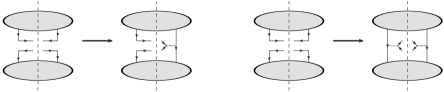
Figure 1: Contributions to the matrix element squared, in which in the left (right) two diagrams one (both) $\text{U}(N_{\text{\tiny C}})$ gluon(s) is (are) replaced by $\text{U}(1)$ gluon(s) on the left or (and) right of the unitarity cut.

For the cases where we include external $\text{U}(1)$ gluons, we use a diagrammatic approach. For each closed colour loop, we have a power of $N_{\text{\tiny C}}$ and each $\text{U}(1)$ gluon comes with a factor of $-1/N_{\text{\tiny C}}$. Hence, we only need to consider the cases with up to two external $\text{U}(1)$ gluons in total in the amplitude and conjugate amplitude.

When introducing external $\text{U}(1)$ gluons, there can be two types of connections between the amplitude and conjugate amplitude: one in which the $\text{U}(1)$ gluon in the dual amplitude connects to a $\text{U}(N_{\text{\tiny C}})$ gluon in the conjugate amplitude (or vice versa), or a $\text{U}(1)$ gluon connects with a $\text{U}(1)$ gluon, see the left and right sets of diagrams in Fig. 1, respectively. The possibility depicted on the left of this figure reduces the number of total closed colour loops by one and introduces one factor of $-1/N_{\text{\tiny C}}$, in total reducing the power of $N_{\text{\tiny C}}$ by 2. For the right part of Fig. 1, the total number of loops is conserved, while two factors of $-1/N_{\text{\tiny C}}$ are introduced. Hence, also in this case there is a total reduction of powers of $N_{\text{\tiny C}}$ by 2. Hence, these two possibilities give NLC contributions if all the other Kronecker deltas give the maximum allowed number of colour loops. That means that the colour ordering must be the same in the amplitude and the conjugate amplitude. This results precisely in the two cases presented. In the following we describe how to use Eq. (61) to further reduce the number of conjugate amplitude per dual amplitude.

We consider the possibility of an interference with one external $\text{U}(1)$ gluon in both the amplitude and the conjugate amplitude, an interference with both amplitude and conjugate amplitude of the type in the second line in Eq. (3.2). For this to contribute at NLC, an NLC factor of $N_{\text{\tiny C}}^{n-1}$, the same gluon in the amplitude and the conjugate amplitude must be the $\text{U}(1)$ gluon, and the order of the other gluons must be identical, so $\sigma_{k}=\sigma_{l}$ for the permutation of the amplitude and conjugate amplitude respectively, where it is understood that the last element of the permutation denotes the $\text{U}(1)$ gluon. This is a single conjugate amplitude for each dual amplitude of this type yielding a NLC entry in the colour matrix.

Next we consider the interferences where the dual amplitude is with one external $\text{U}(1)$ gluon and the conjugate amplitude with only $\text{U}(N_{\text{\tiny C}})$ gluons. For this to be a NLC contribution of colour factor $-N_{\text{\tiny C}}^{n-1}$, the colour order of the $n-1$ $\text{U}(N_{\text{\tiny C}})$ gluons in the amplitude must be identical to the order of these gluons in the conjugate amplitude, while the $\text{U}(1)$ indices might be any of the $\text{U}(N_{\text{\tiny C}})$ gluon indices in the conjugate amplitude. More precisely, if $\sigma_{k}$ denotes the permutation of the amplitude with one external $\text{U}(1)$ gluon where the final element is always understood as the external $\text{U}(1)$ gluon, then its interference with the permutation $\sigma_{l}$ which preserves the relative ordering of the $n-1$ first elements of $\sigma_{k}$, but the $\sigma_{k}(n)$ index is located in any position in $\sigma_{l}$, yields a NLC factor. This is a total of $n$ conjugate amplitudes to consider for each dual amplitude with one external $\text{U}(1)$ gluon. Hence, the sum of these interferences can be written as

$$\begin{split}-N_{\text{\tiny C}}^{n-1}\mathcal{A}_{1qq}(q,\sigma_{k}(1),\ldots,\sigma_{k}(n-1),\overline{q},\sigma_{k}(n))\times&\left[(\mathcal{A}_{1qq}(q,\sigma_{k}(n),\sigma_{k}(1),\ldots,\sigma_{k}(n-1),\overline{q}))^{*}+\right.\\ &\left.(\mathcal{A}_{1qq}(q,\sigma_{k}(1),\sigma_{k}(n),\ldots,\sigma_{k}(n-1),\overline{q}))^{*}+\right.\\ &\left.\ldots\right.\\ &\left.(\mathcal{A}_{1qq}(q,\sigma_{k}(1),\ldots,\sigma_{k}(n-1),\sigma_{k}(n),\overline{q}))^{*}\right]\end{split}$$ (63)

where we note that the sum in the square brackets is precisely the linear combination of the one $\text{U}(1)$-type amplitude $\mathcal{A}_{1qq}(q,\sigma_{k}(1)...\sigma_{k}(n-1),q,\sigma_{k}(n))^{*}$ as given also in Eq. (61). Therefore, this contribution cancels precisely the only interference which appears in the colour matrix between a $\text{U}(1)$ and $\text{U}(1)$ type amplitude with colour factor $+N_{\text{\tiny C}}^{n-1}$ which was discussed in the previous paragraph. As such, these contributions may freely be omitted completely from the colour matrix without changing the colour sum.

Finally, there is the interference between a dual amplitude with all $\text{U}(N_{\text{\tiny C}})$ gluons and a conjugate amplitude with one $\text{U}(1)$ gluon. The possible conjugate amplitudes yielding a NLC are those for which any of the gluons in the amplitude are a $\text{U}(1)$ in the conjugate amplitude, but the relative ordering of the remaining $\text{U}(N_{\text{\tiny C}})$ gluons are unchanged. This results in $n$ possible conjugate amplitude to each dual amplitude of this type. These interferences appear with a factor of $-N_{\text{\tiny C}}^{n-1}$, of the form

$$\begin{split}-N_{\text{\tiny C}}^{n-1}\mathcal{A}_{1qq}(q,\sigma_{k}(1),\ldots,\sigma_{k}(n),\overline{q})\times&\left[(\mathcal{A}_{1qq}(q,\sigma_{k}(2),\sigma_{k}(3),\ldots,\sigma_{k}(n),\overline{q},\sigma_{k}(1)))^{*}+\right.\\ &\left.(\mathcal{A}_{1qq}(q,\sigma_{k}(1),\sigma_{k}(3),\ldots,\sigma_{k}(n),\overline{q},\sigma_{k}(2)))^{*}+\right.\\ &\left.\ldots\right.\\ &\left.(\mathcal{A}_{1qq}(q,\sigma_{k}(1),\sigma_{k}(2),\ldots,\sigma_{k}(n-1),\overline{q},\sigma_{k}(n)))^{*}\right]\end{split}$$ (64)

where in each interference, the $\text{U}(1)$ part of the $\text{U}(N_{\text{\tiny C}})$ gluon in the dual amplitude with the index which the $\text{U}(1)$ gluon carries in the conjugate amplitude, is projected out, reducing the interference of the type with one external $\text{U}(1)$ gluon in both the dual amplitude and the conjugate amplitude. Thus, these interference terms may be moved to the diagonal part of the colour matrix with one external $\text{U}(1)$ gluon amplitude types. The only subtlety is that the colour factor appearing in these diagonal entries are now $-nN_{\text{\tiny C}}^{n-1}$, which accounts for the $n$ rows in the colour matrix with amplitudes with only $\text{U}(N_{\text{\tiny C}})$ gluons which interfere with each of the columns of the colour matrix with a specific gluon ordering and single $\text{U}(1)$ gluon index.

Using the same reasoning we see that an interference type with an amplitude with only $\text{U}(N_{\text{\tiny C}})$ gluons and a conjugate amplitude with two external $\text{U}(1)$ gluons, the number of colour loops will be reduced by two while simultaneously introducing two factors of $-1/N_{\text{\tiny C}}$, hence, this type of interference will not yield a NLC colour factor. This completes the proof.

3.3 Two distinct-flavour $q\overline{q}$ pairs and $n$ gluons

The new feature for amplitudes with two quark lines, is that we must allow for the possibility that the intermediate gluon between the two quark lines is a $\text{U}(1)$ gluon. This is similar to the decomposition of the internal gluon in the fundamental basis in Eq (31) in terms of the Fierz identity. This implies already an explicit $-1/N_{\text{\tiny C}}$ contribution from the internal $\text{U}(1)$ gluon propagator. In particular, the amplitude can be written in the same manner as in the fundamental decomposition [7]

$$\mathcal{M}_{2qq}=\mathcal{M}_{1}-\frac{1}{N_{\text{\tiny C}}}\mathcal{M}_{2},$$ (65)

with the amplitudes

$$\mathcal{M}_{1}=g^{n+2}\sum_{\sigma\in S_{n+1}}c_{1}(\sigma)\mathcal{A}_{1}(\sigma)\quad\textrm{and}\quad\mathcal{M}_{2}=g^{n+2}\sum_{\sigma\in S_{n+1}}c_{2}(\sigma)\mathcal{A}_{2}(\sigma),$$ (66)

and with the colour factors $c_{1,2}$ and dual amplitudes $\mathcal{A}_{1,2}$ defined as

$$\begin{split}c_{1}(\sigma)&=\delta^{i_{q_{1}}}_{j_{\sigma(1)}}\ldots\delta^{i_{\sigma(n_{1})}}_{j_{q_{2}}}\delta^{i_{q_{2}}}_{j_{\sigma(n_{1}+1)}}\ldots\delta^{i_{\sigma(n)}}_{j_{q_{1}}},\\ c_{2}(\sigma)&=\delta^{i_{q_{1}}}_{j_{\sigma(1)}}\ldots\delta^{i_{\sigma(n_{1})}}_{j_{q_{1}}}\delta^{i_{q_{2}}}_{j_{\sigma(n_{1}+1)}}\ldots\delta^{i_{\sigma(n)}}_{j_{q_{2}}},\\ \mathcal{A}_{1}(\sigma)&=\mathcal{A}_{2qq}(q_{1},\sigma(1),\ldots,\sigma(n_{1}+1),\ldots,\sigma(n+1),\overline{q}_{1}),\\ \mathcal{A}_{2}(\sigma)&=\mathcal{A}_{2qq}(q_{1},\sigma(1),\ldots,\sigma(n_{1}+1),\ldots,\sigma(n+1),\overline{q}_{2}).\end{split}$$ (67)

Note, in particular, the difference in the order of the anti-quarks in the colour factors. The dual amplitudes are the same ones appearing in the fundamental basis in Eq (34). Similarly to the case of the two quark lines in the fundamental basis, the sum over permutations $\sigma\in S_{n+1}$ in Eq. (66) includes the permutations of the $n$ gluons, and the $\overline{q}_{2}q_{2}$ pair for $\mathcal{M}_{1}$ and $\overline{q}_{1}q_{2}$ pair for $\mathcal{M}_{2}$, respectively, represented by the element $\sigma(n_{1}+1)$ as before, and therefore $n_{1}$ labels the number of $\text{U}(N_{\text{\tiny C}})$ gluons before the quark-anti-quark pair index.

On top of this, one must also consider external $\text{U}(1)$ gluons by applying the replacement in Eq. (58) to each of the external gluons in both terms. However, as in the case of the one quark pair, we only need to consider up to one external $\text{U}(1)$ gluon to obtain the NLC accurate terms, see Fig. 1 and the discussion around it. Moreover, following similar arguments, it can be directly concluded that having both an internal and an external $\text{U}(1)$ gluon in a dual amplitude cannot result in colour factors that contribute at NLC. Hence, we only need to consider up to one external $\text{U}(1)$ gluon for the $\mathcal{M}_{1}$ term only:

$$\mathcal{M}_{1}\to\mathcal{M}_{1}-\frac{1}{N_{\text{\tiny C}}}g^{n+2}\sum_{\bar{\sigma}\in\bar{S}_{n+1}}c_{1}^{1}(\bar{\sigma})\mathcal{A}_{1}^{1}(\bar{\sigma}),$$ (68)

where

$$\begin{split}c_{1}^{1}(\bar{\sigma})&=\delta^{i_{q_{1}}}_{j_{\sigma(1)}}\ldots\delta^{i_{\sigma(n)}}_{j_{q_{1}}}\delta^{i_{\sigma(n+1)}}_{j_{\sigma(n+1)}},\\ \mathcal{A}_{1}^{1}(\bar{\sigma})&=\mathcal{A}_{2qq}(q_{1},\bar{\sigma}(1),\ldots,\bar{\sigma}(n),\overline{q}_{1},\bar{\sigma}(n+1)),\end{split}$$ (69)

and the set of permutations $\bar{S}_{n+1}$ is the subset of the complete set of permutations $S_{n+1}$ for which $\bar{\sigma}(n+1)$ does not corresponds to the $\overline{q}_{2}q_{2}$ pair. Hence, we have

$$\mathcal{M}_{2qq}=g^{n+2}\left(\sum_{\sigma\in S_{n+1}}c_{1}(\sigma)\mathcal{A}_{1}(\sigma)-\frac{1}{N_{\text{\tiny C}}}\sum_{\sigma_{\in}S_{n+1}}c_{2}(\sigma)\mathcal{A}_{2}(\sigma)-\frac{1}{N_{\text{\tiny C}}}\sum_{\bar{\sigma}\in\bar{S}_{n+1}}c_{1}^{1}(\bar{\sigma})\mathcal{A}_{1}^{1}(\bar{\sigma})\right),$$ (70)

where we have neglected terms that do not contribute up to NLC accuracy.

We obtain then the colour-summed squared amplitude, in block matrix notation,

$$|\mathcal{M}_{2qq}|^{2}=(g^{2})^{n+2}\sum_{\sigma_{k},\sigma_{l}}\begin{pmatrix}\mathcal{A}_{1}(\sigma_{k})&\mathcal{A}_{2}(\sigma_{k})&\mathcal{A}_{1}^{1}(\bar{\sigma}_{k})\end{pmatrix}\\ \begin{pmatrix}c_{1}(\sigma_{k})c_{1}(\sigma_{l})^{\dagger}&-c_{1}(\sigma_{k})c_{2}(\sigma_{l})^{\dagger}\!/N_{\text{\tiny C}}&-c_{1}(\sigma_{k})c_{1}^{1}(\bar{\sigma}_{l})^{\dagger}\!/N_{\text{\tiny C}}\\ -c_{2}(\sigma_{k})c_{1}(\sigma_{l})^{\dagger}\!/N_{\text{\tiny C}}&c_{2}(\sigma_{k})c_{2}(\sigma_{l})^{\dagger}\!/N_{\text{\tiny C}}^{2}&c_{2}(\sigma_{k})c_{1}^{1}(\bar{\sigma}_{l})^{\dagger}\!/N_{\text{\tiny C}}^{2}\\ -c_{1}^{1}(\bar{\sigma}_{k})c_{1}(\sigma_{l})^{\dagger}\!/N_{\text{\tiny C}}&c_{1}^{1}(\bar{\sigma}_{k})c_{2}(\sigma_{l})^{\dagger}\!/N_{\text{\tiny C}}^{2}&c_{1}^{1}(\bar{\sigma}_{k})c_{1}^{1}(\bar{\sigma}_{l})^{\dagger}\!/N_{\text{\tiny C}}^{2}\end{pmatrix}\begin{pmatrix}\mathcal{A}_{1}(\sigma_{l})^{*}\\ \mathcal{A}_{2}(\sigma_{l})^{*}\\ \mathcal{A}_{1}^{1}(\bar{\sigma}_{l})^{*}\end{pmatrix},$$ (71)

where, with some abuse of notation, we have written it with a double sum over $\sigma_{k}$ and $\sigma_{l}$, with the corresponding subpermutations $\bar{\sigma}_{k}$ and $\bar{\sigma}_{l}$ understood.

Leading colour

The leading-colour contribution comes from the similar structure as for the one-quark-line case, i.e. the upper-left block of Eq. (71)

$$\mathcal{A}_{2qq}(q_{1},\sigma_{k}(1),\ldots,\sigma_{k}(n_{1}),\overline{q}_{2}q_{2},\sigma_{k}(n_{1}+2),\ldots,\sigma_{k}(n),\overline{q}_{1})\times\\ \left(\mathcal{A}_{2qq}(q_{1},\sigma_{l}(1),\ldots,\sigma_{l}(n_{1}),\overline{q}_{2}q_{2},\sigma_{l}(n_{1}+2),\ldots,\sigma_{l}(n),\overline{q}_{1})\right)^{*},$$ (72)

with $\sigma_{k}=\sigma_{l}$. This comes with a colour factor equal to

$$\delta^{i_{q_{1}}}_{j_{\sigma_{k}(1)}}\delta^{i_{\sigma_{k}(1)}}_{j_{\sigma_{k}(2)}}\ldots\delta^{i_{\sigma_{k}(n+1)}}_{j_{q_{1}}}\left(\delta^{i_{q_{1}}}_{j_{\sigma_{l}(1)}}\delta^{i_{\sigma_{l}(1)}}_{j_{\sigma_{l}(2)}}\ldots\delta^{i_{\sigma_{l}(n+1)}}_{j_{q_{1}}}\right)^{\dagger}=N_{\text{\tiny C}}^{n+2}.$$ (73)

Next-to-leading colour

Next-to-leading colour contributes as $\pm N_{\text{\tiny C}}^{n}$ (with an exception mentioned below), where the $\pm$ corresponds to the sign of the terms in the colour matrix of Eq. (71). We consider each of the blocks in that colour matrix separately.

• The upper-left block has a similar structure as to the one quark pair case, albeit with an additional $\overline{q}_{2}q_{2}$ pair in the permutations. This can give a NLC contribution if and only if

  $$\sigma_{R}\sigma_{Q_{1}}\sigma_{S}\sigma_{Q_{2}}\sigma_{P}\times\left(\sigma_{R}\sigma_{Q_{2}}\sigma_{S}\sigma_{Q_{1}}\sigma_{P}\right)^{\dagger}.$$ (74)

• The upper-middle and middle-left blocks are interference contributions in which the quark order in the dual amplitude and conjugate amplitude is different. Similarly to the fundamental basis (c.f. upper-right and lower-left blocks of Eq. (37)) these terms can contribute at NLC. Let

  $$\sigma_{A}=\sigma(1),\ldots,\sigma(n_{1})\quad\textrm{and}\quad\sigma_{B}=\sigma(n_{1}+2),\ldots,\sigma(n+1),$$ (75)

  that is, the gluon subpermutations of $\sigma_{k}$ (i.e. the dual amplitude) before and after the quark-pair index, respectively. In order for the $\sigma_{l}$ permutation to give a NLC contribution, it must be that

  $$\sigma_{C}= \sigma_{A}^{1}\sigma_{B}^{2}\quad\textrm{and}\quad\sigma_{D}=\sigma_{B}^{1}\sigma_{A}^{2},$$ (76)

  where $\sigma_{C}$ and $\sigma_{D}$ are, respectively, the subpermutations of the gluons before and after the quark-pair index of the $\sigma_{l}$ permutation, i.e. of the conjugate dual amplitude. The superscripts 1 (2) denote the first (second) subpermutation after splitting the $\sigma_{A,B}$ in two in any possible way, including one of the parts being the empty permutation.

• The lower-right block is the contribution in which both the amplitude and the conjugate amplitude have an external $\text{U}(1)$ gluon. It contributes at NLC with entries $-(n+1)N_{\text{\tiny C}}^{n}$ in the colour matrix if and only if $\bar{\sigma}_{k}=\bar{\sigma}_{l}$.

• The lower-left block contains interference contributions in which only the amplitude has an external $\text{U}(1)$ gluon. The quark order is identical for the amplitude and the conjugate amplitude, and therefore this is very similar to the one-quark-pair case. These terms are canceled in the colour matrix, owing to the reduction of the same type as in Eq. (61) but for the two-quark-pair correspondence.

• The center block comes with an explicit $1/N_{\text{\tiny C}}^{2}$ suppression, and can therefore only contribute to NLC with $N_{\text{\tiny C}}^{n}$ if the strings of Kronecker deltas result in $n+2$ colour loops. This happens only if $\sigma_{k}=\sigma_{l}$.

• Finally, the middle-right and lower-middle blocks only contribute beyond NLC.

This completes all the blocks of Eq. (71).

Proof of the NLC terms

Let us start by discussing the upper-middle and middle-left blocks. That is, for which the anti-quark ordering is different in the dual amplitudes and conjugate amplitudes. The colour factors already come with an explicit $1/N_{\text{\tiny C}}$ suppression. Furthermore, due to the different ordering of the anti-quark indices, the corresponding Kronecker deltas cannot form $n+2$ colour loops: there will be at least one loop made from four Kronecker deltas resulting in a maximum of $n+1$ loops. That introduces another reduction of at least $1/N_{\text{\tiny C}}$ in comparison to LC. Therefore, in order for these terms to contribute at NLC, all the other $2n$ Kronecker deltas must yield $n+1$ colour loops. This can only happen if the subpermutation that corresponds to these Kronecker deltas is identical in the dual amplitude and conjugate amplitude. In other words, apart from a single split and interchange, the $\sigma_{C}$ and $\sigma_{D}$ subpermutations must be identical to $\sigma_{A}$ and $\sigma_{B}$, respectively, see eq. (76).

Similarly to the one-quark-line case the lower-left and the upper-right blocks can be reduced and absorbed in the lower-left block. For the lower-left block, the interference contributes at NLC if and only if the colour order of the $n-1$ $\text{U}(N_{\text{\tiny C}})$ gluons and $\overline{q}_{2}q_{2}$ pair in the amplitude is identical to the order of these gluons and $\overline{q}_{2}q_{2}$ pair in the conjugate amplitude, while the $\text{U}(1)$ gluon might be inserted at any location as a $\text{U}(N_{\text{\tiny C}})$ gluon in the order of the conjugate amplitude. This yields a total of $n+1$ possible conjugate amplitudes. In the same manner as was done in the one-quark pair case, these interferences can however be reduced, since in a single row with a dual amplitude of $\mathcal{A}_{1}^{1}$ type, all interferences between amplitudes of type $\mathcal{A}_{1}$ which yield a NLC is

$$\begin{split}-N_{\text{\tiny C}}^{n}\mathcal{A}_{2qq}(q_{1},\bar{\sigma}_{k}(1),\ldots,\bar{\sigma}_{k}(n),&\overline{q}_{1},\bar{\sigma}_{k}(n+1))\times\\ &\left[(\mathcal{A}_{2qq}(q_{1},\bar{\sigma}_{k}(n+1),\sigma_{k}(1),\ldots,\bar{\sigma}_{k}(n),\overline{q}_{1}))^{*}+\right.\\ &\left.(\mathcal{A}_{2qq}(q_{1},\sigma_{k}(1),\bar{\sigma}_{k}(n+1),\ldots,\ldots,\bar{\sigma}_{k}(n),\overline{q}_{1}))^{*}+\right.\\ &\left.\ldots\right.\\ &\left.(\mathcal{A}_{2qq}(q_{1},\sigma_{k}(1),\ldots,\ldots,\bar{\sigma}_{k}(n),\bar{\sigma}_{k}(n+1),\overline{q}_{1}))^{*}\right]\end{split}$$ (77)

where in the square parenthesis the sum is precisely that of $(\mathcal{A}_{2qq}(q_{1},\bar{\sigma}_{k}(1),\ldots,\bar{\sigma}_{k}(n),\overline{q}_{1},\bar{\sigma}_{k}(n+1)))^{*}$. Therefore, the sum of these contributions cancel the interference in the lower-right block.

A similar analysis is done for the upper-right block, with a dual amplitude of $\mathcal{A}_{1}$ and conjugate amplitudes of $\mathcal{A}_{1}^{1}$ types. Exactly as in the one-quark pair case, these can be reduced to be included in the diagonal elements in the lower-right block, with colour factor $-(n+1)N_{\text{\tiny C}}^{n}$. This completes the proof.

3.4 Two same-flavour $q\overline{q}$ pairs and $n$ gluons

For the same-flavour two-quark-line case in the colour-flow decomposition the arguments follow closely those of the fundamental basis. However, now we must also include external $\text{U}(1)$ gluon emission in the quark ordered amplitudes. For the NLC contributions, it is sufficient to consider only single $\text{U}(1)$ emission. Using the same notation as in the distinct-flavour case in the previous section, we have

$$\mathcal{M}_{1}= g^{n+2}\sum_{\sigma\in S_{n+1}}c_{1}(\sigma)\mathcal{A}_{1}(\sigma)-\frac{1}{N_{\text{\tiny C}}}g^{n+2}\sum_{\bar{\sigma}\in\bar{S}_{n+1}}c_{1}^{1}(\bar{\sigma})\mathcal{A}_{1}^{1}(\bar{\sigma}),$$ (78)

$$\mathcal{M}_{2}= g^{n+2}\sum_{\sigma\in S_{n+1}}c_{2}(\sigma)\mathcal{A}_{2}(\sigma)-\frac{1}{N_{\text{\tiny C}}}g^{n+2}\sum_{\bar{\sigma}\in\bar{S}_{n+1}}c_{2}^{1}(\bar{\sigma})\mathcal{A}_{2}^{1}(\bar{\sigma}).$$ (79)

Symmetrising the distinct-flavour results, we can write the amplitude as

$$\mathcal{M}_{2qq}=\left(1+\frac{1}{N_{\text{\tiny C}}}\right)g^{n+2}\bigg{(}\sum_{\sigma\in S_{n+1}}c_{1}(\sigma)\mathcal{A}_{1}(\sigma)-\frac{1}{N_{\text{\tiny C}}}\sum_{\bar{\sigma}\in\bar{S}_{n+1}}c_{1}^{1}(\bar{\sigma})\mathcal{A}_{1}^{1}(\bar{\sigma})-\\ \sum_{\sigma\in S_{n+1}}c_{2}(\sigma)\mathcal{A}_{2}(\sigma)+\frac{1}{N_{\text{\tiny C}}}\sum_{\bar{\sigma}\in\bar{S}_{n+1}}c_{2}^{1}(\bar{\sigma})\mathcal{A}_{2}^{1}(\bar{\sigma})\bigg{)}.$$ (80)

This yields a colour-summed squared amplitude, in block matrix notation, equal to

$$\begin{split}&|\mathcal{M}_{2qq}|^{2}=(g^{2})^{n+2}\left(1+\frac{1}{N_{\text{\tiny C}}}\right)^{2}&\sum_{\sigma_{k},\sigma_{l}}\begin{pmatrix}\mathcal{A}_{1}(\sigma_{k})&\mathcal{A}_{2}(\sigma_{k})&\mathcal{A}_{1}^{1}(\bar{\sigma}_{k})&\mathcal{A}_{2}^{1}(\bar{\sigma}_{k})\end{pmatrix}\mathbb{C}\begin{pmatrix}\mathcal{A}_{1}(\sigma_{l})^{*}\\ \mathcal{A}_{2}(\sigma_{l})^{*}\\ \mathcal{A}_{1}^{1}(\bar{\sigma}_{l})^{*}\\ \mathcal{A}_{2}^{1}(\bar{\sigma}_{l})^{*}\end{pmatrix}\end{split}$$ (81)

with the colour matrix

$$\mathbb{C}=\begin{pmatrix}c_{1}(\sigma_{k})c_{1}(\sigma_{l})^{\dagger}&-c_{1}(\sigma_{k})c_{2}(\sigma_{l})^{\dagger}&-c_{1}(\sigma_{k})c_{1}^{1}(\bar{\sigma}_{l})^{\dagger}\!/N_{\text{\tiny C}}&c_{1}(\sigma_{k})c_{2}^{1}(\bar{\sigma}_{l})^{\dagger}\!/N_{\text{\tiny C}}\\ -c_{2}(\sigma_{k})c_{1}(\sigma_{l})^{\dagger}&c_{2}(\sigma_{k})c_{2}(\sigma_{l})^{\dagger}&-c_{2}(\sigma_{k})c_{1}^{1}(\bar{\sigma}_{l})^{\dagger}\!/N_{\text{\tiny C}}&-c_{2}(\sigma_{k})c_{2}^{1}(\bar{\sigma}_{l})^{\dagger}\!/N_{\text{\tiny C}}\\ -c_{1}^{1}(\bar{\sigma}_{k})c_{1}(\sigma_{l})^{\dagger}\!/N_{\text{\tiny C}}&c_{1}^{1}(\bar{\sigma}_{k})c_{2}(\sigma_{l})^{\dagger}\!/N_{\text{\tiny C}}&c_{1}^{1}(\bar{\sigma}_{k})c_{1}^{1}(\bar{\sigma}_{l})^{\dagger}\!/N_{\text{\tiny C}}^{2}&-c_{1}^{1}(\bar{\sigma}_{k})c_{2}^{1}(\bar{\sigma}_{l})^{\dagger}\!/N_{\text{\tiny C}}^{2}\\ c_{2}^{1}(\bar{\sigma}_{k})c_{1}(\sigma_{l})^{\dagger}\!/N_{\text{\tiny C}}&-c_{2}^{1}(\bar{\sigma}_{k})c_{2}(\sigma_{l})^{\dagger}\!/N_{\text{\tiny C}}&-c_{2}^{1}(\bar{\sigma}_{k})c_{1}^{1}(\bar{\sigma}_{l})^{\dagger}\!/N_{\text{\tiny C}}^{2}&c_{2}^{1}(\bar{\sigma}_{k})c_{2}^{1}(\bar{\sigma}_{l})^{\dagger}\!/N_{\text{\tiny C}}^{2}\end{pmatrix}.$$ (82)

We notice that in this case, the colour factors are no longer strictly monomials in $N_{\text{\tiny C}}$, but rather a monomial times $(1+1/N_{\text{\tiny C}})^{2}$. As in the fundamental decomposition, we consider contributions to be next-to-leading colour if they are up to $1/N_{\text{\tiny C}}^{2}$-suppressed from the leading-colour one, hence they are of order $\mathcal{O}(N_{\text{\tiny C}}^{n+1})$ and/or $\mathcal{O}(N_{\text{\tiny C}}^{n})$.

Leading colour

Only the first and second diagonal blocks of the colour matrix, Eq. (82), contribute at LC, and only if $\sigma_{k}=\sigma_{l}$.

Next-to-leading colour

Comparing the colour matrix in Eq. (82) with the colour matrix obtained in the distinct-flavour case in Eq. (71), the only really new terms that appear are those with colour factors: $c_{2}^{1}(\bar{\sigma}_{k})c_{1}(\bar{\sigma}_{l})^{\dagger}\!/N_{\text{\tiny C}}$ and $c_{2}^{1}(\bar{\sigma}_{k})c_{1}^{1}(\bar{\sigma}_{l})^{\dagger}\!/N_{\text{\tiny C}}^{2}$ , and the corresponding conjugate cases. However, none of these new colour factors yield a NLC element. The remaining blocks in the last row of the colour matrix are $-c_{2}^{1}(\bar{\sigma}_{k})c_{2}(\bar{\sigma}_{l})^{\dagger}\!/N_{\text{\tiny C}}$ and the diagonal $c_{2}^{1}(\bar{\sigma}_{k})c_{2}^{1}(\bar{\sigma}_{l})^{\dagger}\!/N_{\text{\tiny C}}^{2}$. The sum of the former contributions can be combined to cancel the contribution from the latter type, as was performed in the distinct flavour case. Finally, the conjugate terms $-c_{2}(\bar{\sigma}_{k})c_{2}^{1}(\bar{\sigma}_{l})^{\dagger}\!/N_{\text{\tiny C}}$ are re-located to the diagonal terms of the $-c_{2}^{1}(\bar{\sigma}_{k})c_{2}^{1}(\bar{\sigma}_{l})^{\dagger}\!/N_{\text{\tiny C}}^{2}$ block with the entry $-(n+1)N_{\text{\tiny C}}^{n}$.

Furthermore, for the other elements in the colour matrix, we have different explicit $1/N_{\text{\tiny C}}$ suppression w.r.t. the colour matrix of the distinct-flavour case. However, these differences are at most only one power of $1/N_{\text{\tiny C}}$, while different contractions of the strings of deltas comes with two powers of $1/N_{\text{\tiny C}}$. Using the definition of NLC to contain terms of $\mathcal{O}(N_{\text{\tiny C}}^{n+1})$ and $\mathcal{O}(N_{\text{\tiny C}}^{n})$, but not $\mathcal{O}(N_{\text{\tiny C}}^{n-1})$, there are no additional pieces arising as compared to the distinct-flavour case and the arguments given in there apply here without the need for any modification.

4 Results

In this section we present the main result of this work by showing the number of dual amplitudes which need to be computed in order to calculate scattering probabilities at NLC accuracy. That is, the number of terms in the double sum of Eq. (1) that needs to be considered to get a result that is correct up to NLC accuracy at tree-level.

4.1 Phase-space symmetrisation

Since final state identical particles are indistinguishable, interchanging the momenta of these particles in the numerical phase-space integration must yield identical matrix elements. This fact can be used to reduce the number of terms in the sum of Eq. (1) that needs to be computed, irrespective of the expansion in colour. For example, for $gg\to(n-2)\,g$ scattering, there is a $1/(n-2)!$ symmetry factor due to the $n-2$ identical final state gluons. Therefore, if the phase-space generation in the numerical integration is symmetric under interchange of any two of these gluons, the sum over $k$ (or $l$) can be reduced by the $(n-2)!$ factor, since, upon integration, these rows (or columns) will yield identical results to the cross section and differential distributions [35].

The number of identical final state gluons ($n_{g}$), quarks ($n_{q}$) and anti-quarks ($n_{\bar{q}}$) depend on the scattering process under consideration. In Tab. 1 we list these values for the different types of QCD-particle-initiated processes, together with the total number of dual amplitudes (the number of rows/columns of the colour matrix). The number of non-zero elements in the colour matrix in the fundamental and colour-flow decompositions, including the phase-space symmetrisation, is discussed in the following.

Process	Total (fund.)	Total (colour-flow)	$n_{g}$	$n_{q}$	$n_{\bar{q}}$
$gg\rightarrow(n-2)\,g$	$(n-1)!$	$(n-1)!$	$n-2$	0	0
$gg\rightarrow q\overline{q}+(n-2)\,g$	$n!$	$n!\sum_{r=0}^{n}\frac{1}{r!}$	$n-2$	0	0
$gg\rightarrow q\overline{q}Q\overline{Q}+(n-2)\,g$	$2(n+1)!$	$2n!\sum_{r=0}^{n}\frac{1}{r!}(n+1-r)$	$n-2$	0	0
$gg\rightarrow q\overline{q}q\overline{q}+(n-2)\,g$	$2(n+1)!$	$2n!\sum_{r=0}^{n}\frac{1}{r!}(n+1-r)$	$n-2$	2	2
$qg/\overline{q}g\rightarrow q/\overline{q}+(n-1)\,g$	$n!$	$n!\sum_{r=0}^{n}\frac{1}{r!}$	$n-1$	0	0
$qg/\overline{q}g\rightarrow q/\overline{q}\ Q\overline{Q}+(n-1)\,g$	$2(n+1)!$	$2n!\sum_{r=0}^{n}\frac{1}{r!}(n+1-r)$	$n-1$	0	0
$qg\rightarrow qq\overline{q}+(n-1)\,g$	$2(n+1)!$	$2n!\sum_{r=0}^{n}\frac{1}{r!}(n+1-r)$	$n-1$	2	0
$\overline{q}g\rightarrow q\overline{q}\overline{q}+(n-1)\,g$	$2(n+1)!$	$2n!\sum_{r=0}^{n}\frac{1}{r!}(n+1-r)$	$n-1$	0	2
$q\overline{q}\rightarrow n\,g$	$n!$	$n!\sum_{r=0}^{n}\frac{1}{r!}$	$n$	0	0
$q\overline{q}\rightarrow Q\overline{Q}/q\overline{q}+n\,g$	$2(n+1)!$	$2n!\sum_{r=0}^{n}\frac{1}{r!}(n+1-r)$	$n$	0	0
$qQ/q\overline{Q}\rightarrow qQ/q\overline{Q}+n\,g$	$2(n+1)!$	$2n!\sum_{r=0}^{n}\frac{1}{r!}(n+1-r)$	$n$	0	0
$qq\rightarrow qq+n\,g$	$2(n+1)!$	$2n!\sum_{r=0}^{n}\frac{1}{r!}(n+1-r)$	$n$	2	0
$\overline{q}\overline{q}\rightarrow\overline{q}\overline{q}+n\,g$	$2(n+1)!$	$2n!\sum_{r=0}^{n}\frac{1}{r!}(n+1-r)$	$n$	0	2

Table 1: The total number of rows in the colour matrix in the fundamental (second column) and colour-flow (third column) decomposition for various multi-parton processes at hadron colliders. The number of identical final state gluons ($n_{g}$) and final state quarks ($n_{q}$) and anti-quarks ($n_{\bar{q}}$) are given in the last three columns.

Fundamental decomposition

The total number of independent rows in the colour matrix after phase-space symmetrisation for various processes is given by

$$\frac{N}{n_{g}!\,n_{q}!\,n_{\bar{q}}!},$$ (83)

with $N$ the total number of rows, listed in the second column of Tab. 1, and the number of identical final state gluons $n_{g}$ and the symmetry factor from identical final state quarks $n_{q}$ and anti-quarks $n_{\bar{q}}$, listed in the last three columns of Tab. 1.

Colour-flow decomposition

As shown in Tab. 1, the size of the colour matrix for all-gluon processes is the same in the colour-flow decomposition as in the fundamental decomposition, and the reduction due to the phase-space symmetrisation is the same as in Eq. (83). For amplitudes with external quark lines, however, the case is more subtle. For processes with one quark line plus $n$ gluons the number of amplitudes differs due to the possibility for external $\text{U}(1)$ gluons, which are considered as different dual amplitudes than their corresponding $\text{U}(N_{\text{\tiny C}})$ counterparts. The total number of dual amplitudes in this case is

$$n!\sum_{r=0}^{n}\frac{1}{r!}$$ (84)

where the sum is over the number of external $\text{U}(1)$ gluons in the amplitude. The factors $1/r!$ take into consideration that the $\text{U}(1)$ gluons, being colourless particles, do not take part in the colour-ordering and therefore their permutations do not yield different dual amplitudes. We can rewrite Eq. (84) as

$$\sum_{r=0}^{n}\,\sum_{k=k_{\textrm{min}}}^{k_{\textrm{max}}}\binom{n_{g}}{k}\binom{n-n_{g}}{r-k}(n-r)!$$ (85)

where $k$ is the number of $\text{U}(1)$ gluons among the $n_{g}$ final state gluons, and the sum over $k$ is therefore between $k_{\textrm{min}}=\text{max}(0,r-(n-n_{g}))$ and $k_{\textrm{max}}=\text{min}(r,n_{g})$.

The reduction due to the symmetrisation of the phase-space applies to all final state gluons, irrespective if they are $\text{U}(1)$ and $\text{U}(N_{\text{\tiny C}})$ gluons. However, care must be taken since permutations among the $\text{U}(1)$ gluons yield identical dual amplitudes, which is already taken into account in Eqs. (84) and (85). Hence, the reduction is only equal to $k!/n_{g}!$. Therefore, the total number of independent rows for processes with one quark pair is

$$\sum_{r=0}^{n}\,\sum_{k=k_{\textrm{min}}}^{k_{\textrm{max}}}\binom{n_{g}}{k}\binom{n-n_{g}}{r-k}(n-r)!\frac{k!}{n_{g}!}.$$ (86)

At NLC we only have zero or one external $\text{U}(1)$ gluon, i.e. $r=0,1$, and the sum in Eq. (86) simplifies considerably to $2n!/n_{g}!$.

In the two-quark-line amplitudes, one similarly has to take into consideration the external $\text{U}(1)$ gluons but also the partition of gluons among the colour lines. The total number of dual amplitudes is

$$2n!\sum_{r=0}^{n}\frac{1}{r!}(n+1-r),$$ (87)

with the factor $(n+1-r)$ considering the partition of the gluons on the two colour lines. Comparing this expression to Eq. (84), results in

$$\frac{2}{n_{q}!\,n_{\bar{q}}!}\sum_{r=0}^{n}\,\sum_{k=k_{\textrm{min}}}^{k_{\textrm{max}}}\binom{n_{g}}{k}\binom{n-n_{g}}{r-k}(n-r)!\frac{k!}{n_{g}!}(n+1-r),$$ (88)

independent rows in the colour matrix when taking the phase-space symmetrisation into account for gluons and (anti-)quarks. Note that there is one subtlety regarding the (anti-)quark symmetry factors. For the two-quark-line same-flavour case in the $gg$ initiated process, we have a quark symmetry factor of $n_{q}!\,n_{\bar{q}}!=4$. We note however that not all contributions to the dual amplitudes recover this symmetry. In particular, the case where all gluons are $\text{U}(1)$ gluons, the interchange of the quark labels $q_{1}\leftrightarrow q_{2}$, $\overline{q}_{1}\leftrightarrow\overline{q}_{2}$ recovers the same amplitude, since the two colour lines are now identical with no $\text{U}(N_{\text{\tiny C}})$ gluons attached. Hence, to obtain the number of independent rows in this case, one must divide by the symmetry factor $n_{q}!\,n_{\bar{q}}!=4$ only the contributions with $r=0,\ldots,n-1$ and divide by 2 the $r=n$ contribution.

4.2 Number of non-zero elements in the colour matrix

We start this section by presenting the number of dual conjugate amplitudes that need to be considered for the computation of a single dual amplitude to yield all contributions up to NLC accuracy. In other words this corresponds to computing the number of non-zero elements in a single row (or column) in the colour matrix defined in Eq. (1) up to NLC accuracy. This combined with the number of independent rows due to phase-space symmetrisation, as discussed in the previous section, yields the total number of terms that need to be considered.

all-gluon
$n$	Fundamental		Colour-flow		Adjoint
4	6	(6)	6	(6)	2	(2)
5	11	(24)	16	(24)	5	(6)
6	24	(120)	36	(120)	18	(24)
7	50	(720)	71	(720)	93	(120)
8	95	(5040)	127	(5040)	583	(720)
9	166	(40320)	211	(40320)	4162	(5040)
10	271	(362880)	331	(362880)	31649	(40320)
11	419	(3628800)	496	(3628800)	-
12	620	(39916800)	716	(39916800)	-
13	885	(479001600)	1002	(479001600)	-
14	1226	(6227020800)	1366	(6227020800)	-

Table 2: Number of non-zero elements in a single row of the colour matrix for all-gluon matrix elements up to NLC accuracy, $\mathcal{O}(N_{c}^{n-2})$, in the fundamental, colour-flow and adjoint bases (the latter only up to $n=10$ for computational time reasons). The number between brackets is the total number of elements, i.e. the number needed when full-colour is desired.

In Tab. 2 we present the number of non-zero terms in a single row of the colour matrix for the all-gluon matrix elements. The first column lists the number of gluons in the process. In the second column the number of non-zero terms at NLC are presented using the fundamental basis, while in the third column the same is presented for the colour-flow basis. For completeness, in the final column we also show the number of terms needed in the adjoint representation to obtain NLC accuracy (for numerical reasons, only up to $n=10$). For the three cases, the number in brackets is the total number of elements in a single row, i.e., the number that needs to be computed to obtain full-colour accuracy. It is interesting to note that the scaling with $n$, the number of gluons, is reduced from factorial (the numbers in brackets) to polynomial, $n^{4}$, in both the fundamental and colour-flow bases when considering the matrix elements only up to NLC accuracy. Somewhat surprisingly, in the adjoint basis there is no such reduction and the number of terms still scales factorially. This means that even though this basis is optimal when computing the full-colour matrix elements, since there are only $(n-2)!$ terms, as compared to the $(n-1)!$ in the fundamental and colour-flow bases, this is no longer true at NLC accuracy with multiple gluons. Comparing the fundamental and colour-flow bases, it can be seen that the fundamental basis is slightly more efficient: there are fewer non-zero elements in a single row of the colour matrix to compute. As explained in Secs. 2.1 and 3.1, the reason is the list of exceptions to the general rule that interchanging a single subpermutation of a (string of) generators gives a NLC contribution when using the fundamental basis. A similar rule applies to the colour-flow basis, but without the exceptions, resulting in the need to compute slightly more terms.

$q\overline{q}+n\,g$
$n$	Fundamental		Colour-flow
			no external $\text{U}(1)$		one external $\text{U}(1)$
2	2	(2)	2	(5)	1	(5)
3	4	(6)	6	(16)	1	(16)
4	10	(24)	16	(65)	1	(65)
5	24	(120)	36	(326)	1	(326)
6	51	(720)	71	(1957)	1	(1957)
7	97	(5040)	127	(13700)	1	(13700)
8	169	(40320)	211	(109601)	1	(109601)
9	275	(362880)	331	(986410)	1	(986410)
10	424	(3628800)	496	(9864101)	1	(9864101)
11	626	(39916800)	716	(108505112)	1	(108505112)
12	892	(479001600)	1002	(1302061345)	1	(1302061345)

Table 3: Number of non-zero elements in a single row of the colour matrix for $q\overline{q}+n\,g$ matrix elements up to NLC accuracy, $\mathcal{O}(N_{c}^{n-1})$, in the fundamental and colour-flow bases. The number between brackets is the total number of elements, i.e. the number needed when full-colour is desired. For the colour-flow basis, we distinguish the cases in which the row in the colour matrix corresponds to an amplitude with no external $\text{U}(1)$ gluon, or with one external $\text{U}(1)$ gluon.

In Tab. 3 we present the number of dual conjugate amplitudes that need to be computed for a single dual amplitude to obtain NLC accuracy for $q\overline{q}+n\,g$ matrix elements. In the first column, there is the number of gluons $n$ present in the scattering process. The second column lists the number of non-zero terms in a single row of the colour matrix when using the fundamental basis, with the total number of terms in the row in brackets. For the colour-flow basis, we need to distinguish if the corresponding dual amplitude contains an external $\text{U}(1)$ gluon or not, since the number of conjugate amplitudes that need to be considered is different in the two cases. In the fundamental basis, there are a total number of $n!$ different amplitudes. Hence, for a full colour computation all these contribute to a single row of the colour matrix, and is given in brackets in the second column of the table. The number of conjugate amplitudes is reduced to a polynomial $n^{4}$ scaling when reducing the colour accuracy to NLC, just as in the case of all-gluon matrix elements. In the colour-flow basis, if the dual amplitude does not contain any $\text{U}(1)$ gluons, the NLC terms are produced if the colour ordering of the conjugate amplitude has the form given by Eq. (62). This also reduces the number of terms to a polynomial $n^{4}$ scaling. On the other hand, if the amplitude contains a (single) $\text{U}(1)$ gluon, using the reduction presented in Sec. 3.2, all interferences are moved to the diagonal of these rows, leaving only one conjugate amplitude (column) needed for each row of this type. Note that in the full-colour approach, the number of terms that need be considered scales worse than in the fundamental basis, since not only all permutation of colour ordering for the gluons need be considered (which results in the $n!$ number of terms of the fundamental basis), but also all the replacements of $\text{SU}(N_{c})$ gluons by $\text{U}(1)$ gluons must be taken into account.

$q\overline{q}\,Q\overline{Q}\,+\,n\,g$				Fundamental:  $\mathcal{A}_{1}$ — $\mathcal{A}_{2}$ types
$n$	$\min(n_{1},n-n_{1})$
	$0$		$1$		$2$		$3$		$4$		$5$
0	2 —	2											(2)
1	3 —	3											(4)
2	7 —	4	6 —	5									(12)
3	15 —	5	15 —	7									(48)
4	31 —	6	32 —	9	33 —	10							(240)
5	60 —	7	62 —	11	64 —	13							(1440)
6	108 —	8	111 —	13	114 —	16	115 —	17					(10080)
7	182 —	9	186 —	15	190 —	19	192 —	21					(80640)
8	290 —	10	295 —	17	300 —	22	303 —	25	304 —	26			(725760)
9	441 —	11	447 —	19	453 —	25	457 —	29	459 —	31			(7257600)
10	645 —	12	652 —	21	659 —	28	664 —	33	667 —	36	668 —	37	(79833600)

Table 4: Number of non-zero elements in a single row of the colour matrix for $q\overline{q}\,Q\overline{Q}\,+\,n\,g$ (distinct flavours) up to NLC accuracy, $\mathcal{O}(N_{c}^{n})$, in the fundamental basis. The various columns $\min(n_{1},n-n_{1})$ correspond to the smallest number of gluons of the two partitions $n_{1}$ and $n-n_{1}$ as defined in Eq. (34). Within a column, the number before (after) the vertical bar correspond to a dual amplitude of type $\mathcal{A}_{1}$ ($\mathcal{A}_{2}$), see Eq. (34). The numbers between brackets in the final column denote the total number of columns in the colour matrix. In bold are marked those numbers which appear twice in the mirrored partition.

$q\overline{q}\,Q\overline{Q}\,+\,n\,g$						Colour-flow:  $\mathcal{A}_{1}$, $\mathcal{A}^{1}_{1}$ — $\mathcal{A}_{2}$ types
$n$	$\min(n_{1},n-n_{1})$
	$0$			$1$			$2$			$3$			$4$			$5$
0	2 ,	-  —	2																(2)
1	4 ,	1  —	3																(6)
2	9 ,	1  —	4	10 ,	1  —	5													(22)
3	20 ,	1  —	5	22 ,	1  —	7													(98)
4	41 ,	1  —	6	44 ,	1  —	9	45 ,	1  —	10										(522)
5	77 ,	1  —	7	81 ,	1  —	11	83 ,	1  —	13										(3262)
6	134 ,	1  —	8	139 ,	1  —	13	142 ,	1  —	16	143 ,	1  —	17							(23486)
7	219 ,	1  —	9	225 ,	1  —	15	229 ,	1  —	19	231 ,	1  —	21							(191802)
8	340 ,	1  —	10	347 ,	1  —	17	352 ,	1  —	22	355 ,	1  —	25	356 ,	1  —	26				(1753618)
9	506 ,	1  —	11	514 ,	1  —	19	520 ,	1  —	25	524 ,	1  —	29	526 ,	1  —	31				(17755382)
10	727 ,	1  —	12	736 ,	1  —	21	743 ,	1  —	28	748 ,	1  —	33	751 ,	1  —	36	752 ,	1  —	37	(197282022)

Table 5: Number of non-zero elements in a single row of the colour matrix for $q\overline{q}\,Q\overline{Q}\,+\,n\,g$ (distinct flavours) up to NLC accuracy, $N_{\text{\tiny C}}^{n}$, in the colour-flow basis. The various columns $\min(n_{1},n-n_{1})$ correspond to the smallest number of gluons of the two partitions $n_{1}$ and $n-n_{1}$ as defined in Eq. (67). Within a column, the numbers correspond to dual amplitudes of types $\mathcal{A}_{1}$, $\mathcal{A}_{1}^{1}$ and, after the vertical bars, $\mathcal{A}_{2}$, see Eqs. (67) and (69). The numbers between brackets in the final column denote the total number of columns in the colour matrix. In bold are marked those numbers which appear twice in the mirrored partition.

The number of dual conjugate amplitudes that need to be computed for a single dual amplitude at NLC for the two-quark-pair (distinct-flavour) matrix elements are listed in Tabs. 4 and 5 in the fundamental and colour-flow decompositions, respectively. In the tables, each row corresponds to the number of gluons in the process, denoted in the first column. The various columns ($\min(n_{1},n-n_{1})$) represent the different gluon partitions on the two colour lines, using always the smallest number of gluons on one colour line as label, see also Eq. (34). Furthermore, the number of dual conjugate amplitudes that contribute at NLC also depends on the quark ordering in the amplitude, with the numbers before and after the vertical bars corresponding to the $\mathcal{A}_{1}$ and $\mathcal{A}_{2}$ ordering, respectively. In the case of the colour-flow decomposition, Tab. 5, this number also depends on whether the dual amplitude contains an external $\text{U}(1)$ gluon ($\mathcal{A}_{1}^{1}$) or not. The numbers for the cases when the dual amplitude is a $\mathcal{A}_{1}$ amplitude and $\mathcal{A}_{1}^{1}$ amplitude, are separated by a comma in the table. In each of the tables, the number in the final column in brackets correspond to the total number of dual conjugate amplitudes that need to be considered in the full-colour calculation, i.e. the total number of columns in the colour matrix. The corresponding tables for the same-flavour case can be obtained in the following way: in the fundamental decomposition, both the number of dual conjugate amplitudes for a row with $\mathcal{A}_{1}$- and $\mathcal{A}_{2}$-type diagrams is the same as the number corresponding to a $\mathcal{A}_{1}$-type dual amplitude in Tab.  4, and in the colour-flow decomposition, the number in both the $\mathcal{A}_{1}$- and $\mathcal{A}_{2}$-type columns is the same as the number of $\mathcal{A}_{1}$-type columns in Tab.  5, and similarly both the numbers in the $\mathcal{A}^{1}_{1}$- and $\mathcal{A}^{1}_{2}$-type columns is the same as the numbers presented in the $\mathcal{A}_{1}^{1}$ columns in Tab. 5.

Similarly as to the cases of the all-gluon and one-quark-pair matrix elements, the total number of conjugate dual amplitudes in the two-quark-pair case also scales factorially with the number of gluons involved in the matrix elements, when considering the full colour accuracy. The total number is the same in the distinct-flavour and same-flavour cases, but is considerably worse in the colour-flow basis as compared to the fundamental basis. As before, the reason is the need for the extra dual amplitudes with the external $\text{U}(1)$ gluons in the colour-flow decomposition. Limiting the matrix elements to NLC accuracy greatly decreases the number of contributing dual conjugate amplitudes for a single dual amplitude. In fact, for the worst case, the scaling is still only like a polynomial of degree $4$. However, this depends on the type of dual amplitude for which this number is computed. In the distinct-flavour case, the scaling with the $\mathcal{A}_{2}$ type is only linear with the number of gluons $n$; only the $\mathcal{A}_{1}$ shows the $n^{4}$ scaling. While there are small differences depending on the partition of gluons on the two colour lines in the colour ordering, the scaling is independent from this. For the same-flavour matrix elements there is, of course, no difference for the $\mathcal{A}_{1}$ and $\mathcal{A}_{2}$ dual amplitude types.

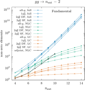
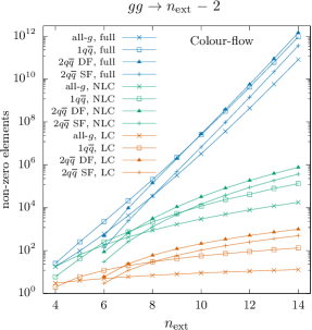
Figure 2: Number of non-zero elements in the colour matrix at LC (red), NLC (green) and full colour (blue) for $gg$ initial state in fundamental (left) and colour-flow decomposition (right) for various channels: all-gluon (cross), one-quark-pair (box), two-quark-pair distinct-flavour (triangle) two-quark-pair same-flavour (bar). In the left figure is also shown the number of non-zero elements in the adjoint decomposition at NLC accuracy up to 10 external particles.

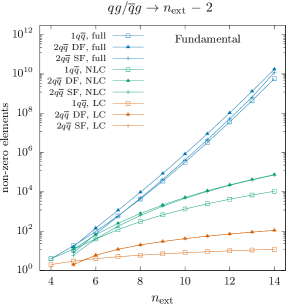
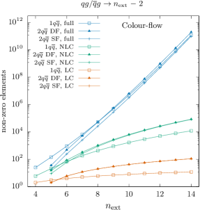
Figure 3: Number of non-zero elements in the colour matrix at LC (red), NLC (green) and full colour (blue) for $qg/\overline{q}g$ initial state in fundamental (left) and colour-flow decomposition (right) for various channels: one-quark-pair (box), two-quark-pair distinct-flavour (triangle) two-quark-pair same-flavour (bar).

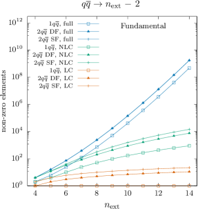
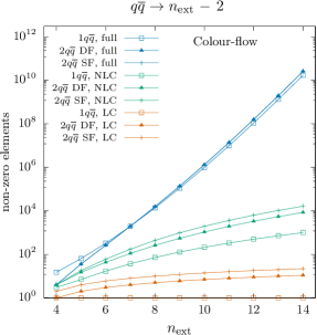
Figure 4: Number of non-zero elements in the colour matrix at LC (red), NLC (green) and full colour (blue) for $q\overline{q}$ initial state in fundamental (left) and colour-flow decomposition (right) for various channels: one-quark-pair (box), two-quark-pair distinct-flavour (triangle) two-quark-pair same-flavour (bar).

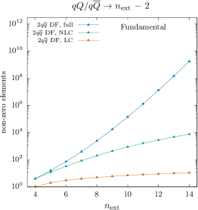
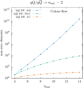
Figure 5: Number of non-zero elements in the colour matrix at LC (red), NLC (green) and full colour (blue) for $qQ/q\overline{Q}$ initial state in fundamental (left) and colour-flow decomposition (right) for the two-quark-pair distinct-flavour channel (triangle).

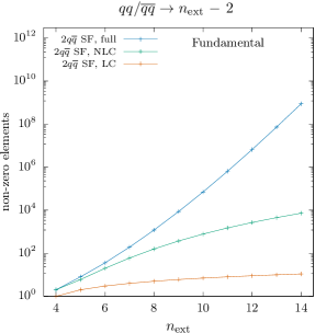
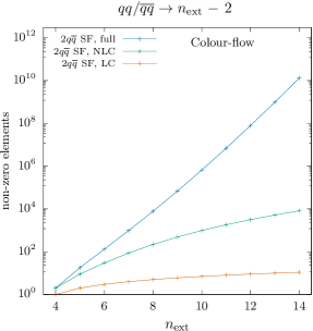
Figure 6: Number of non-zero elements in the colour matrix at LC (red), NLC (green) and full colour (blue) for $qq/\overline{q}\overline{q}$ initial state in fundamental (left) and colour-flow decomposition (right) for the two-quark-pair same-flavour channel (bar).

As discussed above, in Tabs. 2-5 the number of non-zero terms in a single row of the colour matrix are listed. The relevant number of rows, including the reduction due to the symmetrisation of the phase-space, are discussed and given in Sec. 4.1. Hence, this allows us to determine the main results of this work: the total number of elements in the double sum of Eq. (1) that need to be considered to compute matrix elements at NLC accuracy. The results are presented in the form of Figs. 2-6 as a function of the number of external particles, $n_{\rm ext}$. In the figures, the number of non-zero elements at full-colour accuracy is presented with blue curves, at NLC accuracy with green curves, and at leading-colour accuracy with red curves. The curves with crosses correspond to the all-gluon process, the boxes to the processes with one quark line, the triangles to processes with two distinct-flavour quark pairs, and the vertical bars to processes with two same-flavour quark pairs. Figure 2 corresponds to the processes with a $gg$ initial state. The $qg/\overline{q}g$ initial state processes are plotted in Fig. 3. In Fig. 4 the same curves are given for $q\overline{q}$ initial state in the two decompositions and the processes with $qQ/q\overline{Q}$ and $qq/\overline{q}\overline{q}$ initial states are presented in Figs. 5 and 6, respectively. For all these figures, the left plot corresponds to the fundamental decomposition and the right plot to the colour-flow decomposition. In the left figure of Fig. 2 we also present the NLC accurate curve (black) in the adjoint decomposition. For completeness, the data that fills these figures is given in Tabs. 6-10 in Appendix A.

From the figures the following patterns can be deduced.

• The factorial growth of the number of terms with the number of external particles in the full-colour results is clearly visible. This is irrespective of the process considered.

• Similarly, it can be seen that all the (N)LC contributions scale polynomially with the number of partons participating in the scattering process, with the maximum degree at NLC higher than at LC. The exception is the NLC in the adjoint representation for the all-gluon scattering process, which does not show a polynomial scaling.

• The turn-over for the efficiency (number of non-zero terms) between the fundamental (or colour-flow) and the adjoint decomposition for the all-gluon process appears between $n=8$ and $n=9$, including the phase-space symmetrisation.

• The differences between the fundamental and colour-flow decompositions are rather small at (N)LC accuracy, while in the full-colour results the colour-flow basis requires the computation of significantly more terms.

• At all the accuracies (full-colour, NLC and LC) and for each of the initial states, the contributions with the most terms are the two-quark-pair distinct-flavour processes. The reason for this is mostly due to the greater reduction from the phase-space symmetrisation for multi-gluon contributions. The exceptions are the processes with the same-flavour $q\overline{q}$ pair initial states, where the same-flavour two-quark-line processes require more terms. The reason is that additional reduction due to the phase-space symmetrisation for the same-flavour two-quark-line matrix elements is absent.

• In general, already for $2\to 4,5$ processes there are significantly fewer contributions to be considered at NLC than at full-colour (note the squared exponential scale for the $y$-axes in these plots). This suggests that even at relatively low multiplicities the colour expansion up to NLC results in improvements in calculation speed compared to full-colour.

5 Conclusion

We have presented, at tree-level, the rules for obtaining all dual conjugate amplitudes for a given dual amplitude which are needed to perform a NLC accurate computation of scattering probabilities, for all-gluon, one-quark-pair and two-quark-pair processes. By including also the phase-space symmetrisation, we have presented the number of non-zero elements in the NLC accurate colour matrix in both the fundamental and colour-flow decompositions and found that in both cases the number of elements in the colour matrix reduces from the factorial growth (with the number of external particles) at full colour, to a polynomial growth at NLC. This opens a path to a matrix element generator of polynomial complexity, without a need for Monte Carlo sampling over colours.

We have compared the fundamental and colour-flow decompositions and found that the fundamental decomposition is slightly more efficient for making the colour matrix sparse at NLC, which is partly due to additional dual amplitudes with external $\text{U}(1)$ gluons which are present in the colour-flow basis only, and partly due to the fewer exceptions to the general rules in the colour-flow basis. We also compare the sparseness of the colour matrix in these non-minimal bases with the adjoint decomposition for the all-gluon case and find that at $n=9$ gluons or more, the fundamental and colour-flow decompositions are more efficient than the adjoint basis at NLC.

Already for scattering amplitudes at moderate multiplicities, $2\to 4,5$, there are significantly fewer contributions at NLC as compared to full colour. This suggests that this work could also be of practical interest for computing cross sections and differential distributions for LHC scattering processes. It is worth investigating the exact trade-off between the increase in speed and the decrease in accuracy due to omission of contributions beyond NLC. We formally suppress orders of $1/N_{\text{\tiny C}}^{3}$ (corresponding to a few percent; although this might be enhanced for high-multiplicity processes), therefore we expect other sources of uncertainties, such as renormalization scale dependence, to be dominant. An in-depth analysis of this is left for future work.

All the rules for NLC are presented for processes with up two two quark pairs, at tree level only. While the set of rules can be extended to cover also processes with larger number of quark pairs, these processes are phenomenologically less relevant. The loop-level colour structures have been worked out in great detail and available in literature for the all-gluon and multiple-quark-pair cases, however they might pose further levels of complexity for determining the NLC elements in the colour matrix.

The code for the colour computations presented in the paper is available from the authors upon request.

Appendix A Data for figures

In this appendix we list the numbers in Tabs. 6-10 that were used to create Figs. 2-6.

$gg\rightarrow n_{\rm ext}-2$         Fundamental
$n_{\rm ext}$	all-gluon		one-quark		two-quark DF		two-quark SF
4	18	(3)	6	(2)	-		-
5	44	(4)	24	(6)	-		-
6	120	(5)	120	(12)	66	(6)	10	(3)
7	300	(6)	480	(20)	504	(24)	180	(12)
8	665	(7)	1530	(30)	2388	(60)	954	(30)
9	1328	(8)	4074	(42)	8680	(120)	3720	(60)
10	2439	(9)	9464	(56)	26160	(210)	11715	(105)
11	4190	(10)	19800	(72)	68376	(336)	31500	(168)
12	6820	(11)	38160	(90)	159824	(504)	75040	(252)
13	10620	(12)	68860	(110)	341568	(720)	162504	(360)
14	15938	(13)	117744	(132)	678510	(990)	325890	(495)

Table 6: Number of non-zero elements in the colour matrix at NLC and at LC (in parenthesis) including the reduction due to the phase-space symmetrisation, for $gg$ initial states for all-gluon, one-quark-pair and two-quark-pair (same-flavour (SF) and distinct-flavour (DF)) processes for various numbers of final-state particles ($n_{\rm ext}-2$) in the fundamental representation.

$gg\rightarrow n_{\rm ext}-2$         Colour-flow
$n_{\rm ext}$	all-gluon		one-quark		two-quark DF		two-quark SF
4	18	(3)	6	(2)	-		-
5	64	(4)	42	(6)	-		-
6	180	(5)	255	(12)	86	(6)	30	(3)
7	426	(6)	740	(20)	666	(24)	261	(12)
8	889	(7)	2160	(30)	3108	(60)	1302	(30)
9	1688	(8)	5376	(42)	10980	(120)	4870	(60)
10	2979	(9)	11872	(56)	32100	(210)	14685	(105)
11	4960	(10)	23904	(72)	81606	(336)	38124	(168)
12	7876	(11)	44730	(90)	186256	(504)	88256	(252)
13	12024	(12)	78870	(110)	390168	(720)	186884	(360)
14	17758	(13)	132396	(132)	762210	(990)	367740	(495)

Table 7: Number of non-zero elements in the colour matrix at NLC and at LC (in parenthesis) including the reduction due to the phase-space symmetrisation, for $gg$ initial states for all-gluon, one-quark-pair and two-quark-pair (same-flavour (SF) and distinct-flavour (DF)) processes for various numbers of final-state particles ($n_{\rm ext}-2$) in the colour-flow representation.

$qg/\overline{q}g\rightarrow n_{\rm ext}-2$    Fundamental							Colour-flow
$n_{\rm ext}$	one-quark		two-quark DF		two-quark SF		one-quark		two-quark DF		two-quark SF
4	4	(2)	-		-		6	(2)	-		-
5	12	(3)	12	(2)	6	(2)	21	(3)	15	(2)	9	(2)
6	40	(4)	66	(6)	40	(6)	68	(4)	86	(6)	60	(6)
7	120	(5)	252	(12)	180	(12)	185	(5)	333	(12)	261	(12)
8	306	(6)	796	(20)	636	(20)	432	(6)	1036	(20)	876	(20)
9	679	(7)	2170	(30)	1860	(30)	896	(7)	2745	(30)	2435	(30)
10	1352	(8)	5232	(42)	4686	(42)	1696	(8)	6420	(42)	5874	(42)
11	2475	(9)	11396	(56)	10500	(56)	2988	(9)	13601	(56)	12705	(56)
12	4240	(10)	22832	(72)	21440	(72)	4970	(10)	26608	(72)	25216	(72)
13	6886	(11)	42696	(90)	40626	(90)	7887	(11)	48771	(90)	46701	(90)
14	10704	(12)	75390	(110)	72420	(110)	12036	(12)	84690	(110)	81720	(110)

Table 8: Number of non-zero elements in the colour matrix at NLC and at LC (in parenthesis) including the reduction due to the phase-space symmetrisation, for $qg/\overline{q}g$ initial states for one-quark-pair and two-quark-pair (same-flavour (SF) and distinct-flavour (DF)) processes for various numbers of final-state particles ($n_{\rm ext}-2$) in the fundamental and colour-flow representations.

$q\overline{q}\rightarrow n_{\rm ext}-2$    Fundamental							Colour-flow
$n_{\rm ext}$	one-quark		two-quark DF		two-quark SF		one-quark		two-quark DF		two-quark SF
4	2-	(1)	4	(1)	4	(2)	3	(1)	4	(1)	4	(2)
5	4	(1)	12	(2)	12	(4)	7	(1)	15	(2)	18	(4)
6	10	(1)	33	(3)	40	(6)	17	(1)	43	(3)	60	(6)
7	24	(1)	84	(4)	120	(8)	37	(1)	111	(4)	174	(8)
8	51	(1)	199	(5)	318	(10)	72	(1)	259	(5)	438	(10)
9	97	(1)	434	(6)	744	(12)	128	(1)	549	(6)	974	(12)
10	169	(1)	872	(7)	1562	(14)	212	(1)	1070	(7)	1958	(14)
11	275	(1)	1628	(8)	3000	(16)	332	(1)	1943	(8)	3630	(16)
12	424	(1)	2854	(9)	5360	(18)	497	(1)	3326	(9)	6304	(18)
13	626	(1)	4744	(10)	9028	(20)	717	(1)	5419	(10)	10378	(20)
14	892	(1)	7539	(11)	14484	(22)	1003	(1)	8469	(11)	16344	(22)

Table 9: Number of non-zero elements in the colour matrix at NLC and at LC (in parenthesis) including the reduction due to the phase-space symmetrisation, for $q\overline{q}$ initial state for one-quark-pair and two-quark-pair (same-flavour (SF) and distinct-flavour (DF)) processes for various numbers of final-state particles ($n_{\rm ext}-2$) in the fundamental and colour-flow representations.

$qQ/q\overline{Q}$   Fundamental			Colour-flow
$n_{\rm ext}$	two-quark DF		two-quark DF
4	4	(1)	4	(1)
5	12	(2)	15	(2)
6	33	(3)	43	(3)
7	84	(4)	111	(4)
8	199	(5)	259	(5)
9	434	(6)	549	(6)
10	872	(7)	1070	(7)
11	1628	(8)	1943	(8)
12	2854	(9)	3326	(9)
13	4744	(10)	5419	(10)
14	7539	(11)	8469	(11)

$qq/\overline{q}\overline{q}$   Fundamental			Colour-flow
$n_{\rm ext}$	two-quark SF		two-quark SF
4	2	(1)	2	(1)
5	6	(2)	9	(2)
6	20	(3)	30	(3)
7	60	(4)	87	(4)
8	159	(5)	219	(5)
9	372	(6)	487	(6)
10	781	(7)	979	(7)
11	1500	(8)	1815	(8)
12	2680	(9)	3152	(9)
13	4514	(10)	5189	(10)
14	7242	(11)	8172	(11)

Table 10: Number of non-zero elements in the colour matrix at NLC and at LC (in parenthesis) including the reduction due to the phase-space symmetrisation, for $qQ/q\overline{Q}$ (left) and $qq/\overline{q}\overline{q}$ (right) initial states for two-quark-pair processes for various numbers of final-state particles ($n_{\rm ext}-2$) in the fundamental and colour-flow representations.

References

• [1] J. Alwall, R. Frederix, S. Frixione, V. Hirschi, F. Maltoni, O. Mattelaer, H.S. Shao, T. Stelzer, P. Torrielli, M. Zaro, JHEP 07, 079 (2014). DOI 10.1007/JHEP07(2014)079
• [2] R. Frederix, S. Frixione, V. Hirschi, D. Pagani, H.S. Shao, M. Zaro, JHEP 07, 185 (2018). DOI 10.1007/JHEP07(2018)185
• [3] E. Bothmann, et al., SciPost Phys. 7(3), 034 (2019). DOI 10.21468/SciPostPhys.7.3.034
• [4] J. Bellm, et al., Eur. Phys. J. C 76(4), 196 (2016). DOI 10.1140/epjc/s10052-016-4018-8
• [5] S. Alioli, P. Nason, C. Oleari, E. Re, JHEP 06, 043 (2010). DOI 10.1007/JHEP06(2010)043
• [6] M.L. Mangano, S.J. Parke, Z. Xu, Nucl. Phys. B 298, 653 (1988). DOI 10.1016/0550-3213(88)90001-6
• [7] F. Maltoni, K. Paul, T. Stelzer, S. Willenbrock, Phys. Rev. D 67, 014026 (2003). DOI 10.1103/PhysRevD.67.014026
• [8] V. Del Duca, L.J. Dixon, F. Maltoni, Nucl. Phys. B 571, 51 (2000). DOI 10.1016/S0550-3213(99)00809-3
• [9] S. Keppeler, M. Sjodahl, JHEP 09, 124 (2012). DOI 10.1007/JHEP09(2012)124
• [10] T. Gleisberg, S. Hoeche, JHEP 12, 039 (2008). DOI 10.1088/1126-6708/2008/12/039
• [11] G. ’t Hooft, Nucl. Phys. B 72, 461 (1974). DOI 10.1016/0550-3213(74)90154-0
• [12] R. Kleiss, H. Kuijf, Nucl. Phys. B 312, 616 (1989). DOI 10.1016/0550-3213(89)90574-9
• [13] C. Reuschle, S. Weinzierl, Phys. Rev. D 88(10), 105020 (2013). DOI 10.1103/PhysRevD.88.105020
• [14] H. Johansson, A. Ochirov, JHEP 01, 170 (2016). DOI 10.1007/JHEP01(2016)170
• [15] T. Melia, JHEP 12, 107 (2015). DOI 10.1007/JHEP12(2015)107
• [16] A. Ochirov, B. Page, JHEP 10, 058 (2019). DOI 10.1007/JHEP10(2019)058
• [17] Z. Bern, D.A. Kosower, Nucl. Phys. B 362, 389 (1991). DOI 10.1016/0550-3213(91)90567-H
• [18] D. Christie, Information Processing Letters 60, 165 (1995). DOI 10.1016/S0020-0190(96)00155-X
• [19] M.L. Mangano, S.J. Parke, Nucl. Phys. B 299, 673 (1988). DOI 10.1016/0550-3213(88)90368-9
• [20] M.L. Mangano, Nucl. Phys. B 309, 461 (1988). DOI 10.1016/0550-3213(88)90453-1
• [21] M.L. Mangano, S.J. Parke, Phys. Rept. 200, 301 (1991). DOI 10.1016/0370-1573(91)90091-Y
• [22] L.J. Dixon, in Theoretical Advanced Study Institute in Elementary Particle Physics (TASI 95): QCD and Beyond (1996), pp. 539–584
• [23] F. Caravaglios, M.L. Mangano, M. Moretti, R. Pittau, Nucl. Phys. B 539, 215 (1999). DOI 10.1016/S0550-3213(98)00739-1
• [24] D.A. Kosower, Nucl. Phys. B 315, 391 (1989). DOI 10.1016/0550-3213(89)90361-1
• [25] Z. Bern, L.J. Dixon, D.A. Kosower, Nucl. Phys. B 437, 259 (1995). DOI 10.1016/0550-3213(94)00542-M
• [26] R.K. Ellis, W.T. Giele, Z. Kunszt, K. Melnikov, G. Zanderighi, JHEP 01, 012 (2009). DOI 10.1088/1126-6708/2009/01/012
• [27] R.K. Ellis, Z. Kunszt, K. Melnikov, G. Zanderighi, Phys. Rept. 518, 141 (2012). DOI 10.1016/j.physrep.2012.01.008
• [28] H. Ita, K. Ozeren, JHEP 02, 118 (2012). DOI 10.1007/JHEP02(2012)118
• [29] T. Melia, Phys. Rev. D 88(1), 014020 (2013). DOI 10.1103/PhysRevD.88.014020
• [30] T. Melia, Phys. Rev. D 89(7), 074012 (2014). DOI 10.1103/PhysRevD.89.074012
• [31] T. Melia, PoS RADCOR2013, 031 (2013). DOI 10.22323/1.197.0031
• [32] T. Schuster, Phys. Rev. D 89(10), 105022 (2014). DOI 10.1103/PhysRevD.89.105022
• [33] K. Hagiwara, Y. Takaesu, Eur. Phys. J. C 71, 1668 (2011). DOI 10.1140/epjc/s10052-011-1668-4
• [34] S. Frixione, B.R. Webber, (2021)
• [35] S. Badger, B. Biedermann, P. Uwer, V. Yundin, Comput. Phys. Commun. 184, 1981 (2013). DOI 10.1016/j.cpc.2013.03.018