Stellar Evolution confronts Axion Models

Abstract

Axion production from astrophysical bodies is a topic in continuous development, because of theoretical progress in the estimate of stellar emission rates and, especially, because of improved stellar observations. We carry out a comprehensive analysis of the most informative astrophysics data, revisiting the bounds on axion couplings to photons, nucleons and electrons, and reassessing the significance of various hints of anomalous stellar energy losses. We confront the performance of various theoretical constructions in accounting for these hints, while complying with the observational limits on axion couplings. We identify the most favorable models, and the regions in the mass/couplings parameter space which are preferred by the global fit. Finally, we scrutinize the discovery potential for such models at upcoming helioscopes, namely IAXO and its scaled versions.

1 Introduction

The most elegant solution to the strong CP problem, the so called Peccei-Quinn (PQ) mechanism [1, 2], implies the existence of the axion [3, 4], which also provides one of the best particle physics candidates for cold dark matter (DM) [5, 6, 7]. The axion arises as the pseudo Nambu-Goldstone boson of a spontaneously broken global Abelian symmetry endowed with a mixed anomaly with the color gauge group $SU(3)_{c}$, and the couplings and the mass of the axion are inversely proportional to the scale at which spontaneous symmetry breaking occurs. Already shortly after the axion hypothesis was conceived it became clear that this scale had to lie much beyond the electroweak scale, given that no axion signatures could be detected in laboratory experiments, thus implying that axions must be very weakly coupled to ordinary matter and very light. Such light particles could then be produced in the hot and dense plasma of star cores and then freely escape, thus providing an additional channel for energy losses from astrophysical bodies that would affect their evolution. In fact, the strongest limits on axion couplings to electrons, nucleons and electromagnetic radiation come from the requirement that stellar lifetimes and energy-loss rates should not conflict with observations [9, 10, 11]. Astrophysical limits have been derived from the non-observation of axion emission from our Sun, from the concordance between the prediction of stellar evolution codes and direct observations of star distributions in the color-magnitude diagram (CMD) for evolved low-mass star populations, such as red giant branch (RGB) and horizontal-branch (HB) stars in globular clusters, from limits on cooling rates of white dwarfs (WD) and neutron stars (NS), and from the duration of the neutrino burst from the collapsed core of supernova (SN) SN 1987A. These limits have been frequently revised and updated in the literature, with the coming of better observations and more detailed analyses. However, intriguingly, rather than pushing the bounds on the various couplings to smaller and smaller values, the more recent astrophysical observations have hinted at finite, though small, axion couplings. More specifically, a set of astrophysical anomalies seem to indicate a preference for non-vanishing couplings of axions to electrons and, to a lesser extent, to photons. Although individually the significance of each one of these hints is marginal (1 or $2\,\sigma$), there is concordance among all the independent observations when interpreted in terms of axions [10], which raises the overall significance at about the $3\,\sigma$ level. Analyses of other new physics candidates does not show the same level of agreement among the different observations [12], making axions the most interesting candidates to explain the anomalies.

In the last few years, the advent of new observations of remarkably improved accuracy has required the revision of some astrophysical bounds on axions. In particular, the RGB bound on the axion-electron coupling has been considerably improved and the significance of the hint has been reduced [13, 14]. The supernova and neutron star bounds have also been updated in the last few years [15, 16, 17, 18, 19]. In light of these recent progresses, it seems timely to revise the global analysis of the stellar bounds/hints on axions, and to provide updated regions in parameter space where the experimental search may be particularly motivated. This is the task we address in this paper.

Besides a general, model independent analysis of the stellar observables, we carry out dedicated analyses focusing on specific axion models. Going beyond the approach followed in Ref. [10], the present study is not limited to scrutinize only the canonical DFSZ models, but also considers a set of non-universal realizations of DFSZ models, wherein same-type quarks of different generations can couple to different Higgs doublets [20, 21, 22]. In particular, we focus on models that feature the property of nucleo-phobia, i.e. the capability to strongly suppress the axion coupling to nucleons. Given the tight constrains stemming from observations of SN and NS, which strongly bound the axion-nucleon coupling, these models perform particularly well in reproducing the global set of astrophysics data. We will constrain the parameter region and ascertain the quality of the fit for each of the axion models of our representative sample, singling out those constructions that most successfully account for the observations.

As we shall show, the parameter space preferred by stars is the meV mass region (roughly, 1 to 100 meV). Intriguingly, this parameter region is the goal of the next generation of axion helioscopes. In particular, BabyIAXO, expected to be operative in the next few years, may already be able to dig into the parameter space hinted by stars for some QCD axion models. These regions will be better accessible by the full scale IAXO helioscope. The even larger IAXO+ will be able to essentially cover the entire parameter space preferred by stars for most well motivated axion models.

The paper is organized as follows. In Sec. 2 we review the axion effective Lagrangian and we define the coupling of the axion to the SM particles. In Sec. 3 we give an updated summary of the astrophysical observables relevant to our analysis. A review of the models scrutinized in this paper is given in Sec. 4. Our results are reported in Sec. 5, with Sec. 5.1 devoted to a discussion of the constrains on the axion couplings to SM fields in the various models, and Sec. 5.2 dedicated to analyse, for each model, the discovery potential at forthcoming axion search experiments. In Sec. 6 we resume our results and draw the conclusions. A detailed calculation of the axion-photon couplings for the non-universal DFSZ models is presented in Appendix A.

2 Axion effective Lagrangian

In this section we focus on the most relevant axion couplings from the point of view of astrophysics and experimental sensitivities for an axion mass scale ranging in the several meV region. The axion effective Lagrangian including photons and matter fields $f=p,n,e$ (defined at a scale $\Lambda<m_{p}$) can be written as

$$\mathcal{L}_{a}=\frac{1}{2}(\partial_{\mu}a)^{2}-\frac{1}{2}m_{a}^{2}a^{2}+\frac{\alpha}{8\pi}\frac{C_{a\gamma}}{f_{a}}aF_{\mu\nu}\tilde{F}^{\mu\nu}+C_{af}\frac{\partial_{\mu}a}{2f_{a}}\overline{f}\gamma^{\mu}\gamma_{5}f\,,$$ (2.1)

where the adimensional coefficients $C_{a\gamma}$ and $C_{af}$ read [23, 24]

$$C_{a\gamma} =\frac{E}{N}-1.92(4)\,,$$ (2.2)

$$C_{ap} =-0.47(3)+0.88(3)\,C_{u}-0.39(2)\,C_{d}-C_{a,\,{sea}}\,,$$ (2.3)

$$C_{an} =-0.02(3)+0.88(3)\,C_{d}-0.39(2)\,C_{u}-C_{a,\,{sea}}\,,$$ (2.4)

$$C_{a,\,{sea}} =0.038(5)\,C_{s}+0.012(5)\,C_{c}+0.009(2)\,C_{b}+0.0035(4)\,C_{t}\,,$$ (2.5)

$$C_{ae} =C_{e}+\frac{3\alpha^{2}}{4\pi^{2}}\left[\frac{E}{N}\log\left(\frac{f_{a}}{m_{e}}\right)-1.92(4)\log\left(\frac{{\rm GeV}}{m_{e}}\right)\right]\,.$$ (2.6)

In Eqs. (2.2) and (2.6) $E$ and $N$ correspond respectively to the electromagnetic and QCD anomaly coefficients of the PQ current

$$\partial^{\mu}J^{\rm PQ}_{\mu}=\frac{\alpha_{s}N}{4\pi}G^{a}_{\mu\nu}\tilde{G}^{a\,\mu\nu}+\frac{\alpha E}{4\pi}F_{\mu\nu}\tilde{F}^{\mu\nu}\,.$$ (2.7)

The coefficients $C_{\psi}$ (with $\psi$ a SM quark or lepton) can be written as

$$C_{\psi}=c^{0}_{\psi}+\epsilon_{\psi}\,,$$ (2.8)

where $c^{0}_{\psi}$, which is defined in terms of the derivative interaction terms

$$c^{0}_{\psi}\,\frac{\partial_{\mu}a}{2f_{a}}\overline{\psi}\gamma^{\mu}\gamma_{5}\psi\,,$$ (2.9)

denotes the UV axion-fermion couplings as determined from the model-dependent PQ charges, while $\epsilon_{\psi}$ is a correction due to possible fermion mixing effects that will generally arise, after electroweak symmetry breaking, in models in which the PQ charges are generation dependent. In all the models we will consider these corrections are small in the case of the quarks of the first generation. In some cases they can become sizeable for quarks of the second and third generation (see Table 3) but since their contribution as sea quarks to $C_{ap},\,C_{an}$ is already suppressed by small coefficients (see Eq. (2.5)) we can expected that Eqs. (2.3)–(2.4), which are derived under the assumption of no mixing effects, will still remain valid to a good approximation. Finally, in Eq. (2.6) the first term $C_{e}=c^{0}_{e}+\epsilon_{e}$ corresponds to the tree level axion coupling to the electron, while the second term is the one-loop contribution originating from a triangle loop involving two photons [25, 26].

In the following, we will use the following rescaled axion couplings

$$g_{a\gamma}=\frac{\alpha}{2\pi}\frac{C_{a\gamma}}{f_{a}}\,,\qquad g_{af}=C_{af}\frac{m_{f}}{f_{a}}\,,$$ (2.10)

and employ the definitions $g_{\gamma 10}\equiv g_{a\gamma}\times\left(10^{10}\,\text{GeV}\right)$ and $g_{e13}\equiv g_{ae}\times 10^{13}$. Finally the relation between the axion mass and the axion decay constant reads [27]

$$m_{a}=5.691(51)\left(\frac{10^{12}\ \text{GeV}}{f_{a}}\right)\,\text{$\mu$eV}\,.$$ (2.11)

3 Astrophysical observables and cooling anomalies

Astrophysical considerations have played a quite significant role in the investigation of the physics of light, weakly interacting particles, such as neutrinos, dark photons, axions, axion like particles (ALPs) etc. [9]. Constraints derived from the observations of stellar populations are often much tighter than bounds from direct searches. Intriguingly, a series of anomalous astrophysical observations have led to speculations that new physics may be at play in determining the details of stellar evolution [12, 28, 10, 29, 30, 24, 31]. The axion (or ALP) case is especially compelling since, contrarily to other new physics candidates, fits particularly well all astrophysical observations [28, 10]. A list of updated bounds and hints from stellar evolution on the axion couplings are summarized in Table 1. The aim of this Section is to review and update the status of the impact of axion emission on stellar evolution. We begin by reviewing the most relevant axion production mechanisms in stars, and next we summarize the constraints and hints from observations of different stellar systems.

Star	Hint	Bound	Reference
Sun $\Big{|}$	No Hint	$g_{\gamma 10}\leq 2.7$	[32]
WDLF	$g_{e13}=1.5^{+0.3}_{-0.5}$	$g_{e13}\leq 2.1$	[33]
WDV	$g_{e13}=2.9^{+0.6}_{-0.9}$	$g_{e13}\leq 4.1$	[34]
RGBT (22 GGCs)	$g_{e13}=0.60^{+0.32}_{-0.58}$	$g_{e13}\leq 1.5$	[13]
RGBT (NGC 4258)	No Hint	$g_{e13}\leq 1.6$	[14]
HB	$g_{\gamma 10}=0.3^{+0.2}_{-0.2}$	$g_{\gamma 10}\leq 0.65$	[35, 36]
SN 1987A	No Hint	$g_{aN}\lesssim 9.1\!\times\!10^{-10}$	[15]
NS (CAS A)	No Hint	$(g_{ap}^{2}+1.6\,g_{an}^{2})^{1/2}\lesssim 1.0\!\times\!10^{-9}$	[16]
NS (CAS A)	No Hint	$g_{an}\lesssim 3\!\times\!10^{-10}$	[19]
NS (HESS)	No Hint	$g_{an}\leq 2.8\!\times\!10^{-10}$	[17]

Table 1: Updated bounds and hints from stellar evolution on the axion couplings. WDLF: White Dwarf Luminosity Function; WDV: White Dwarf Variables; RGBT: Red Giant Branch Tip; HB: Horizontal Branch; SN: Supernova; NS: Neutron Star. The bound from SN 1987A is on the effective coupling $g_{aN}$ defined in Eq. (3.15). The two RGBT bounds are from two independent analyses, the first one based on 22 galactic globular clusters [13] and the second based on the NGC 4258 galaxy [14]. The three NS bounds are from independent analyses, two based on observations of CAS A [16, 19] and one on observations of HESS J1731-347  [17]. We have not listed the hint from the CAS A study in Ref. [37] since it is in tension with the more recent bounds shown in the Table. In the last column we give the references to the original analyses.

3.1 Axion production in stars

The most relevant axion production mechanisms in stellar environments are the Primakoff, Compton, and electron bremsstrahlung processes. A pedagogical introduction to these processes can be found in Ref. [9], while a set of approximate expressions and numerical results can be found in the appendix of Ref. [38]. Here we just recall a few semi-analytical formulae for axion production through the different processes that will be useful for the following discussion.

In star core plasma with a relatively low density the most relevant axion production mechanisms are the Primakoff and Compton processes. The former is induced by the axion coupling to photons and the latter by its coupling to electrons. The Primakoff process is the photon conversion into an axion in the electric field of electrons or ions in the plasma:

$$\gamma+Ze\to a+Ze\,.$$ (3.1)

Neglecting degeneracy effects and the plasma frequency (a good assumption in environments in which the Primakoff process is the dominating axion production mechanism) it is possible to provide a semi-analytical expression for the energy-loss rate per unit mass due to axion emission [39]:

$$\varepsilon_{P}\simeq 2.8\times 10^{-31}F(\xi)\left(\frac{g_{a\gamma}}{\rm GeV^{-1}}\right)^{2}\frac{T^{7}}{\rho}\,{\rm erg\,g^{-1}\,s^{-1}}\,,$$ (3.2)

where $T$ and $\rho$ are in K and in g cm^-3. The function $F$ depends on the Debye-Huckel screening wavenumber $\kappa_{S}$ via the variable $\xi\equiv\kappa_{S}/2T$, and can be explicitly expressed as an integral over the photon distribution (see Eq. (4.79) in Ref. [40]). An approximate expression, which agrees with numerical results at better than 2% over the entire range of $\xi$, is [39]

$$F(\xi)\simeq\left(\frac{1.037\,\xi^{2}}{1.01+0.185\,\xi^{2}}+\frac{1.037\,\xi^{2}}{44+0.628\,\xi^{2}}\right)\ln\left(3.85+\frac{3.99}{\xi^{2}}\right)\,.$$ (3.3)

In general, $F(\xi)$ is ${\cal O}(1)$ for relevant stellar conditions. More general numerical recipes, valid also in a degenerate medium, can be found in the appendix of Ref. [38].

In general the Primakoff process does not play a significant role in the evolution of superdense star cores, in which case other processes dominate. The Compton process

$$\gamma+e\to\gamma+a$$ (3.4)

accounts for the production of axions from the scattering of thermal photons on electrons. The Compton axion emission rate is a steep function of the temperature:

$$\varepsilon_{\rm C}\simeq 2.7\times 10^{-22}g_{ae}^{2}\frac{1}{\mu_{e}}\left(\frac{n_{e}^{\rm eff}}{n_{e}}\right)\,T^{6}\,{\rm erg\,g^{-1}\,s^{-1}}\,,$$ (3.5)

where $\mu_{e}=\left(\sum X_{j}Z_{j}/A_{j}\right)^{-1}$ is the mean molecular weight per electron with $X_{j}$ the relative mass density of the $j$-th ion and $Z_{j},~{}A_{j}$ its charge and mass number respectively, $n_{e}$ is the number density of electrons while $n_{e}^{\rm eff}$ is the effective number density of electron targets. At high densities, degeneracy effects reduce $n_{e}^{\rm eff}$, suppressing the Compton rate. Thus, this process is particularly effective in high-temperature environments, as long as the density is still relatively low to prevent electron degeneracy (cf. Fig. 1 in [41]). At higher densities and especially when electron degeneracy conditions are reached, the most efficient axion production mechanism is the electron/ion bremsstrahlung process

$$e+Ze\to e+Ze+a\,.$$ (3.6)

For degenerate plasma conditions, the axion energy-loss rates per unit mass can be approximated as

$$\varepsilon_{\rm B}\simeq 8.6\times 10^{-7}F_{B}\,g_{ae}^{2}T^{4}\left(\sum\frac{X_{j}Z_{j}^{2}}{A_{j}}\right){\rm erg\,g^{-1}\,s^{-1}}\,.$$ (3.7)

The mild density dependence of the degenerate rate is accounted for by the dimensionless function $F_{B}$. An explicit expression for this function can be found in [42] (see also Sec. 3.5 of Ref. [9] for a pedagogical presentation). Numerically its value is of order one for the typical stellar plasma conditions in which the degenerate bremsstrahlung process dominates $\rho\sim 10^{5}-10^{6}\,{\rm g\,cm^{-3}}$ and $T\sim 10^{7}-10^{8}\,{\rm K}$.

In a nuclear medium such that of a SN collapsed core or in NS cores, the processes discussed above are generally sub-dominant [43]. If the axion coupling to nucleons is not particularly suppressed, as is the case in most axion models, a more efficient production mechanism is axion bremsstrahlung in nucleon-nucleon collisions

$$N+N^{\prime}\to N+N^{\prime}+a\,,$$ (3.8)

where $N,N^{\prime}=n,p$. If we model the nucleon-nucleon interaction with the exchange of a single pion, it is evident that the pion mass in the propagator will suppress the emission rate, unless the temperature is such that the typical momentum exchanged in the collision, which is of the order of the nucleon momentum $q_{N}\sim(3m_{N}T)^{1/2}$, is larger than the pion mass. This demands $T\gtrsim 10$ MeV, a temperature typical of SN and NS cores. Therefore, among the various stellar objects, SN and NS provide the best environments to test the axion nucleon coupling.

Approximate expressions for the $nn$ scattering emission rates (the $pp$ scattering is similar) in the limit of non-degenerate (ND) and degenerate (D) nuclei are given below [9]

$$\varepsilon_{{\rm ND}}\approx 2.0\times 10^{38}g_{an}^{2}\rho_{14}\,T_{30}^{3.5}\,{\rm erg}\,{\rm g}^{-1}{\rm s}^{-1}\,,$$ (3.9a)

$$\varepsilon_{{\rm D}}\approx 4.7\times 10^{39}g_{an}^{2}\rho_{14}^{-2/3}\,T_{30}^{6}\,{\rm erg}\,{\rm g}^{-1}{\rm s}^{-1}\,,$$ (3.9b)

where $T_{30}=T/30$MeV and $\rho_{14}=\rho/10^{14}{\rm g}\,{\rm cm}^{-3}$. These expression are based on a series of approximations, however, they still provide a good order of magnitude estimate of the axion emission rate from a SN or NS, and in particular they put in evidence the steeper temperature dependence in the case of a degenerate medium. However, throughout this work we use the more accurate numerical results from Ref. [15] (see Sec. 3.5).

3.2 Axion Bounds from White Dwarfs

WDs represent the last stage of the evolution of low mass stars, following the exhaustion of the nuclear fuel. Therefore, during this phase the star is just cooling. WDs are characterized by a dense core of degenerate electrons, with typical density of about $10^{6}$ g cm^-3 and a core temperature dependent on the age of the star. Young WDs are hot and brighter, and cool through volume neutrino emission. At later times, the photon surface cooling dominates.

The addition of exotic particles, such as axions, can have a strong impact on the evolution of the WD, accelerating the stellar cooling. Thus, testing the cooling efficiency is an indirect way to probe the existence of new physics. There are two independent ways to test the cooling efficiency of WDs. One is to observe the WD luminosity function (WDLF), which shows the WD number distribution in different luminosity bins (see Sec. 3.2.1). The other, is to measure changes in the period of WD variables (WDV), a class of WD whose luminosity periodically changes with time (see Sec. 3.2.2).

Both methods indicate a preference for some unidentified cooling, which could well be provided by axion emission provided their coupling to electrons is of a few $10^{-13}$. Below we give more details on the analyses of WD cooling rates.

3.2.1 White Dwarf luminosity function

As we have already mentioned, the WDLF represents the number distribution of WDs as a function of their luminosity. This distribution has been used for decades as a tool to measure the WD cooling efficiency, since the number of WDs with a certain luminosity obviously depends on how efficiently the star looses energy. If axions exist, they would be produced in a WD core primarily through the bremsstrahlung process. Hence, the WDLF has provided information about the axion coupling to electrons (see Ref. [44] for a recent review). Unfortunately, observations from the Sloan Digital Sky Survey (SDSS) and the and SuperCOSMOS Sky Survey (SSD), on which the current studies are based, are not consistent within their quoted error bars, indicating that the systematic uncertainties in these observations might have been underestimated [45]. Consequently, there is no complete consensus on the exact bound on the axion-electron coupling derived from observations of the WDLF. A summary of different studies can be found in Ref. [33]. In that analysis, the authors enlarged the error bars to take into account not only their systematic uncertainties, but also the discrepancies between the SDSS and SSS observations (see discussion therein, in sec. 4.2). In the present study, we adopt the result $g_{ae}\leq 2.1\times 10^{-13}$ at $(2\,\sigma)$, derived in Ref. [33].

Furthermore, most studies of the WDLF seem to indicate an excessive cooling with respect to the standard prediction. Such cooling has been interpreted as due to an axion-electron coupling $g_{ae}\simeq(1.4\pm 0.3)\times 10^{-13}$ (at 1$\sigma$) [33].

3.2.2 White Dwarf Variables

The WDV are a set of WDs whose luminosity changes periodically. The period $P$ ranges from a few to several minutes, depending on the particular star. It is well known that observations of the secular change, $\dot{P}$, of the WDV period provide information about the efficiency of the WD cooling. In fact, to a very good approximation $\dot{P}/P$ is directly proportional to the cooling rate $\dot{T}/T$. Hence, an accurate measurement of $\dot{P}$ allows to set bounds on possible sources of extra cooling (see Ref. [34] for a comprehensive review).

For over two decades, observations of the period decrease ($\dot{P}/P$) of particular WDVs have shown discrepancies with the expected behavior. This is clear from the data in Table 2, which shows the results of the observations of the WDVs analyzed so far [34]. The systematic tendency of the observed $\dot{P}$ to be larger than the expected values can be interpreted in terms of a new particle, produced in the core and efficiently carrying energy outside the star. Even though specific observations have been interpreted in various ways, for example in terms of an anomalously large neutrino magnetic moment (see, e.g., Ref. [49]), a global analysis of all the data indicates a preference for axions among other WISPy candidates [28], and identifies the coupling with electrons in the range $g_{ae}=2.9^{+0.6}_{-0.9}\times 10^{-13}$ (at 1$\sigma$) [10], with a 2$\sigma$ bound of $g_{ae}\leq 4.1\times 10^{-13}$, as reported in Table 1. The analysis in this paper is based on the recent review [34], where the most updated studies on the viable WDV are considered. The results for the axion couplings are summarized in Tab. 2.

We conclude observing that, following the approach usually employed in the literature and first outlined in Ref. [28], we will not include in our fits data relative to the WD G117-B15A: the analysis for this star shares many theoretical similarities to the one relative to R548, but the experimental results are somewhat different, with the hint on $g_{ae}$ stemming from the former noticeably stronger than the one inferred from the latter. Given that results relative to these two WDs are based on very similar hypothesis, we will therefore conservatively include in our fit only data pertaining to R548, along with the data from PG 1351+489 and L 19-2.

Star	$P$(s)	$\dot{P}_{\rm obs}$(s/s)	$\dot{P}_{\rm th}$(s/s)	$g_{ae}^{(\rm best)}$	$g_{ae}^{\rm(max)}(2\sigma)$
G117 - B15A|	215	$(5.5\pm 0.8)\!\times\!10^{-15}$	$(1.25\pm 0.09)\!\times\!10^{-15}$	$5.6\!\times\!10^{-13}$	$6.7\!\times\!10^{-13}$
R548	213	$(3.3\pm 1.1)\!\times\!10^{-15}$	$(1.1\pm 0.09)\!\times\!10^{-15}$	$4.8\!\times\!10^{-13}$	$6.8\!\times\!10^{-13}$
PG 1351+489	489	$(2.0\pm 0.9)\!\times\!10^{-13}$	$(0.81\pm 0.5)\!\times\!10^{-13}$	$2.1\!\times\!10^{-13}$	$3.8\!\times\!10^{-13}$
L 19-2 (113)	113	$(3.0\pm 0.6)\!\times\!10^{-15}$	$(1.42\pm 0.85)\!\times\!10^{-15}$	$5.1\!\times\!10^{-13}$	$7.7\!\times\!10^{-13}$
L 19-2 (192)	192	$(3.0\pm 0.6)\!\times\!10^{-15}$	$(2.41\pm 1.45)\!\times\!10^{-15}$	$2.5\!\times\!10^{-13}$	$6.1\times 10^{-13}$

Table 2: Measured and expected value of $\dot{P}$ for a set of WDV. Here, $P$ is the period of the variable star and $\dot{P}$ its time derivative. The interpretation in terms of axion coupling to electrons is also shown. (Data from Ref. [24] except for G117-B15A, which corresponds to the updated analysis in Ref. [50]).

3.3 Axion Bounds from the tip of RGB stars in globular cluster

After completing the evolution through the main sequence, characterized by a H-burning core, low mass stars begin climbing the RGB, well visible in the color-magnitude diagram as a diagonal line starting at the main sequence and directed toward the colder and higher luminosity region. During the evolution in the RGB, stars are characterized by a He core and a burning H shell, whose ashes increase the He core mass, while the star luminosity (determined by equilibrium at the surface of the He core between thermal pressure supporting the non-degenerate envelope against the gravity pull from the core) keeps growing. The process continues until the core reaches sufficiently large temperatures and densities ($T\sim 10^{8}\,$K, $\rho=10^{6}\,$g cm^-3) to ignite He, an event known as the He-flash. At this stage the star has reached the maximum luminosity, that is the RGB tip (RGBT), after which it shrinks and moves to the HB. If an additional core-cooling mechanism is at play, He ignition is delayed, the core would accrete a larger mass, and the star would reach higher luminosities. Therefore, measurements of the luminosity of the RGB tip allow to test the rate of cooling during the RGB phase. The method is particularly effective for constraining $g_{ae}$ since in red giant cores axions can be efficiently produced via electron bremsstrahlung.

We denote by $M_{I,{\rm TRGB}}$ the luminosity of the tip of the RGB in globular clusters (GC). Following Ref. [41], based on the analysis in Ref. [51, 28], it is possible to derive the following analytical expression for the expected magnitude of the RGBT:

$$M_{I,{\rm TRGB}}^{\rm theo}=-4.08-0.25\bigg{(}\sqrt{g_{e13}^{2}+0.96^{2}}-0.96-0.17g_{e13}^{1.5}\bigg{)}\,,$$ (3.10)

that has an associated theoretical uncertainty $\sigma^{2}={0.039^{2}+(0.046+0.012g_{e13})^{2}}$. This should be compared with the observational values. The latest analyses are those in Refs. [13, 14]. The first, is based on the global analysis of a sample of 22 GC while the second analyzes individual clusters and galaxies. Both studies give very similar results (cf. Table 1). Here, as a reference, we consider the observational value found in the comprehensive analysis from Ref. [13]. This choice results in the bound on the axion-electron coupling $g_{e13}\leq 1.5$ (2$\,\sigma$), which is perfectly compatible with the one found in Ref. [14], but also hints to a non-vanishing value for $g_{e13}$. At any rate, we have verified that removing this additional hint from our fit does not alter significantly the results.

3.4 Helium burning stars

After He ignition, the RG core expands and the star migrates to the horizontal branch of the color magnitude diagram, characterized by a He burning non-degenerate core. The core of a HB star has a density of about $\rho\sim 10^{4}\,{\rm g\,cm^{-3}}$, which is about two orders of magnitude less than that of a RGB star or a WD. In this environment, axions are efficiently produced through the Primakoff and Compton processes. The effect of the additional energy loss provided by axion production and emission is to accelerate the helium consumption in the HB core and, consequently, to reduce the lifetime of this stage. A very efficient way to probe this effect is by measuring the so called $R$ parameter, $R=N_{\rm HB}/N_{\rm RGB}$, which measures the ratio between the number in the HB and in the upper portion of the RGB in GC.

Historically, measurements of the $R$ parameter have been used to derive bounds on the axion-photon coupling [52, 53, 35, 36]. However, the axion electron coupling can also impact the $R$ parameter. Following the results of Refs. [28, 10, 24], we present the expected $R$ parameter in the following form

$$R=R_{0}(Y)-F_{a\gamma}\!\left(g_{\gamma 10}\right)-F_{ae}\!\left(g_{e13}\right)\,,$$ (3.11)

where $R_{0}(Y)$ is a function of the helium abundance ($Y$) in the GC and $F_{a\gamma}$, $F_{ae}$ are some positive-definite functions of the axion couplings. Evidently, the impact of axions on the $R$ parameter may be induced by its couplings with photons as well as by its coupling with electrons. However, surprisingly, there are no explicit stellar numerical evaluation of the $R$ parameter which include both couplings. An approximate expression for the functions $F$, based on a series of older numerical results, was presented in Refs. [28, 10]. There, it was found

$$R_{0}(Y)=0.02+7.33\,Y\,,$$ (3.12)

$$F_{a\gamma}(x)=0.095\sqrt{21.86+21.08\,x}\,,$$ (3.13)

$$F_{ae}(x)=0.0053\,x^{2}+0.039\left(\sqrt{1.23^{2}+x^{2}}-1.23-0.14\,x^{3/2}\right).$$ (3.14)

The theoretical expression in Eq. (3.11) should be compared with observational results, in order to constraint the axion couplings. Ref. [35], reported the value $R=1.39\pm 0.03$ from the analysis of 39 clusters, and used the result to derive the bound $g_{a\gamma}\leq 0.65\times 10^{-10}\,{\rm GeV^{-1}}$ at $2\,\sigma$ [35, 36], under the assumption that the axion couples only to photons.

More massive He burning stars, with mass $M\sim 8-12M_{\odot}$, can also provide some insight into the axion-photon coupling [39, 54]. The (core) He burning stage of these stars is characterized by a migration towards the blue (hotter) region of the CMD and back. This journey is known as the blue loop. The existence of the loop is corroborated by many astronomical observations. In particular, this stage is essential to account for the observed Cepheid stars (see, e.g., Ref. [55]). Ref. [39], based on numerical simulations of solar metallicity stars in the $8-12M_{\odot}$ mass range, showed that a coupling larger than $\approx 0.8\times 10^{-10}{\rm GeV}^{-1}$ would cause the complete disappearance of the blue loop while a somewhat lower values of $g_{a\gamma}$ might help explain the observed deficiency of blue with respect to red supergiants, as is discussed, e.g., in Ref. [56]. The numerous uncertainties in the microphysics and in the numerical description of the blue loop stage, however, have not permitted a more quantitative assessment of this possibility [12]. Hence, these results will be ignored in our present work.

3.5 Supernovae

The observation of the neutrino signal from SN 1987A, and the recent observation of a NS associated with it [57] supported the picture of a neutrino driven SN explosion with neutrinos carrying away about 99% of the energy released in the explosion. Since new weakly coupled particles could accelerate the cooling and reduce the observed duration of the neutrino signal, SN 1987A nutrino data have been widely used to constrain models of new physics, and particularly axion properties [58, 59, 60, 40].

The plasma in the core of a SN, in the first few seconds after the explosion, is extremely hot ($T\sim 30$ MeV) and dense ($\rho\sim 3\times 10^{14}\,$g/cm³). This makes the SN an extremely interesting environment to study new physics. Axions can be produced in this environment through different processes, including the Primakoff process [61, 62, 63], and the electron bremsstrahlung [64]. However, for couplings allowed by other astrophysical considerations the nuclear bremsstrahlung, driven by the axion coupling to neutrons and protons, largely dominates over the latter two. The most recent analysis of the axion-nucleon bremsstrahlung [15] give the bound

$$g^{2}_{aN}\equiv g_{an}^{2}+0.61\,g_{ap}^{2}+0.53\,g_{an}\,g_{ap}\lesssim 8.26\times 10^{-19}\,,$$ (3.15)

which is the one we adopt in the present study. If the axion coupling to nucleons is large enough, axions may be trapped in the SN core [71, 15]. In this case, the cooling efficiency is reduced and the axion bound weakened. Unfortunately, the exact value of the coupling for which axions are sufficiently trapped so that the observed duration of the neutrino signal is not reduced, is afflicted by several uncertainties. However, in most models in which the SM fermions carry a PQ charge the trapping regime is already excluded by other stellar bounds. Thus, in the present work we will not consider further this possibility.

3.6 Neutron stars

Observations of the cooling of NS also provide information about the axion-nucleon coupling [72, 73, 16, 17, 18, 19]. Several NS bounds on $g_{aN}$ exist in the literature, however, they are not always consistent with one another. One of the most studied NS is the one in CAS A. In recent years, there has been some speculation that its anomalously rapid cooling could be a hint of axions with coupling to neutrons [37] $g_{an}\simeq 4\times 10^{-10}$. However, the data can also be explained assuming a neutron triplet superfluid transition occurring at the present time, $t\sim 320$ years, in addition to a proton superconductivity operating at $t\ll 320$ years [16]. Under these assumptions, it was possible to fit the available data well, leaving little room for additional axion cooling, corresponding to the bound [16]:

$$g_{ap}^{2}+1.6\,g_{an}^{2}\leq 1.1\times 10^{-18}\,.$$ (3.16)

A stronger bound, though only on the axion-neutron coupling,

$$g_{an}\leq 2.8\times 10^{-10}\,,$$ (3.17)

was inferred from observations of the NS in HESS J1731-347 [17]. This bound is also in good agreement with a newer analysis of the NS in CAS A carried out in Ref. [19] (cf. Table 1).

In the present work, we take the bound in Eq.(3.17) as a reference for the NS bound on the axion-nucleon coupling. It should be remarked, however, that there is no universal consensus on the NS bound. For example, Ref. [18] recently proposed a considerable less stringent result,

$$g_{an}\lesssim(2.5-3.2)\times 10^{-9}\,.$$ (3.18)

For this reason, we present separate analyses, with and without the NS results.

3.7 Model-independent fit

In this subsection we describe the global fit to the relevant astrophysical observables described above, that we have performed by taking the axion couplings $g_{ae}$ and $g_{a\gamma}$ as uncorrelated parameters. Given the absence of any particular assumption about an underling axion model, this first analysis is denoted as model-independent. Note that this implies that $g_{ae}$ and $g_{a\gamma}$ are not correlated to the couplings to nucleons either, and hence it is consistent to neglect, in the model-independent fit, the data inferred from SNe and NS observations. However, this additional set of data will be taken into account in the model-dependent fits performed in Sec. 5 where, given the model, all the couplings are correlated in a well defined way. In short, in this subsection we will consider only data pertaining to WD, RGB and HB stars.

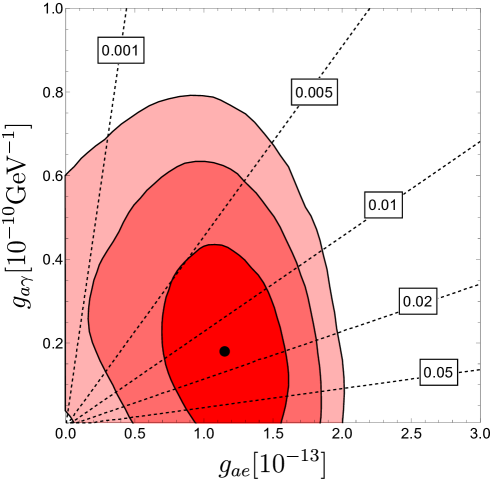
Figure 1: Global bounds from stellar cooling: $1\sigma$ (dark red) to $3\sigma$ (light red). The global mode, corresponding to $g_{e12}=0.1$ and $g_{\gamma 10}=0.2$, is shown as a black dot. Dashed lines represent iso-lines for the ratio $C_{ae}/C_{a\gamma}$.

We depict in Fig. 1 the $1\sigma$, $2\sigma$ and $3\sigma$ regions allowed by the fit, showing also the iso-lines for the ratio $C_{ae}/C_{a\gamma}$. The best fit point is marked with a black dot, and corresponds to $g_{ae}\simeq 1.2\times 10^{-13}$ and $g_{a\gamma}\simeq 0.18\times 10^{-10}\text{GeV}^{-1}$, with $C_{ae}/C_{a\gamma}\simeq\mathcal{O}(10^{-2})$. It is interesting to notice that the present data, including the information relative to HB, can be accommodated by the introduction of a non-vanishing axion-electron coupling only. On the other hand, the SM case ($g_{ae}=g_{a\gamma}=0$) is excluded by present data at the about the $3\sigma$ level.

Let us add a comment regarding a comparison with the global analysis in Ref. [10]. The results of this previous study are qualitatively similar to what is shown in our Fig. 1. The most relevant quantitative difference is the RGB contribution to the global fit. Ref. [10] was based on the RGB analysis in Ref. [51], which adopted an incorrect screening prescription for the nuclear reaction rates [74]. The correction of this numerical issue in Refs. [13, 14] strengthened substantially the bound on the axion-electron coupling, and caused a shift of the entire $g_{ae}$ region in Fig. 1 to the left. As stated in Sec. 3.3, we employed in our fit the results obtained in Ref. [13], but we tested the stability of our findings under this choice performing also a fit where we used the results from Ref. [14]. We found that the contours of the preferred regions differ only slightly between the two choices, with the SM case always excluded at the $\sim 3\sigma$ level. The results shown in Fig. 1 therefore give a reliable representation of the region preferred by the stars.

As anticipated above, in Sec. 4 we will review a selection of motivated axion models, each of which will imply specific correlations among the various axion couplings in terms of a few model parameters. The impact of the stellar evolution data on the corresponding bounds and the effectiveness of those specific models in accommodating the hints for extra energy emission from stars are discussed in Sec. 5.

4 A representative sample of axion models

In this Section we introduce a set of explicit axion models which yield different axion couplings to the nucleons, the electrons and the photons. In Sec. 5.1 we will consider how well they can perform in addressing the issue of possible anomalies in stellar energy losses, accommodating the observational hints while respecting all other phenomenological bounds.

The model-independent analysis of Sec. 3.7 suggests that promising candidates among axion models should comply with a first requirement of predicting a sizeable $C_{ae}/C_{a\gamma}$ ratio. For this reason KSVZ models [75, 76], in which the $C_{ae}$ coupling arises radiatively from a triangle loop involving two photons, and hence is induced by $C_{a\gamma}$, are not well suited to explain the cooling hints. Indeed, for KSVZ models one obtains

$$\frac{C_{ae}}{C_{a\gamma}}\simeq\frac{3\alpha^{2}}{4\pi^{2}}\frac{\frac{E}{N}\log\left(\frac{f_{a}}{m_{e}}\right)-1.92\log\left(\frac{{\rm GeV}}{m_{e}}\right)}{E/N-1.92}\simeq\frac{3\alpha^{2}}{4\pi^{2}}\log\left(\frac{f_{a}}{m_{e}}\right)\simeq 1.1\times 10^{-4}\,,$$ (4.1)

where in the next-to-last relation we have selected the log-enhanced contribution and assumed $E/N\gg 1.92$, and in the last relation we have chosen as reference value $f_{a}=10^{9}$ GeV. As it can be seen from Fig. 1, the iso-line $C_{ae}/C_{a\gamma}=10^{-3}$ already misses the 1$\sigma$ region preferred by the global fit, so that the KSVZ value of $10^{-4}$ cannot provide a good fit to the stellar cooling hints. Hence, we will not considered the KSVZ model any further in the present study.

A better starting point for addressing the cooling hints is provided by DFSZ models [77, 78] since the axion coupling to electrons arises at tree level. In particular, the nucleo-phobic axion models of Refs. [20, 21, 22, 79] allow to relax astrophysical bounds from NS/SN, while keeping at the same time a sizeable coupling to electrons and photons. An additional motivation to consider the latter class of models consists in the fact that their generation dependent PQ charge assignment is engineered in such a way that the contributions of two generations to the QCD anomaly factor cancel out yielding $N=N_{1}+N_{2}+N_{3}=N_{1}$. This implies a DW number $N_{\rm DW}=2N_{1}=2$ or 1 (rather than $N_{\rm DW}=2N=6$ or 3 as in canonical DFSZ models) [20]. The importance of the existence of DFSZ-like models with $N_{\rm DW}=1$ consists in the fact that they are strongly preferred in post-inflationary PQ-breaking scenarios since they are free from the DW problem. In this case in fact the network of axionic strings coupled to a single DW spontaneously decays around the time when the axion acquires a mass. In this scenario, under the assumption that the shape of the instantaneous axion emission from string decays is IR dominated [80, 81], cosmological considerations based on the requirement that the axion relic density will not exceed that of the DM, together with the requirement that axion interactions will be sufficiently suppressed to impede axion thermalization into dark radiation, yield a viable window for the axion mass between 0.2 and 100 meV [82]. As can be seen from Table 4 in Sec. 5.1, this agrees well with the mass window favoured by the cooling hints.

In this Section we first review the basic features of the above-mentioned DFSZ-like axion models, and next we generalize further the classification of axion models with two Higgs doublets and generation dependent PQ charges by including novel constructions. In particular, we show that models featuring particularly large coupling to photons and electrons can still be nucleo-phobic, a feature that allows to optimize the fit to the cooling anomalies while bringing the corresponding axions within the discovery potential of future helioscopes such as (Baby)IAXO. In spite of the fact that we analyze a reasonably large number of different constructions, we stress that our list is far from representing the entire panorama of axion models. In particular, it leaves out models in which the axion coupling to electrons can be enhanced by specific mechanisms (see e.g. [86, 87, 88]). Nevertheless, it is unlikely that these alternative possibilities could yield much better fits to the hinted anomalies than our representative subset. This is because the best fit conditions are realised when $g_{ae}/g_{a\gamma}\approx 0.6\times 10^{-2}\,$GeV and $g_{ap},\,g_{an}\approx 0$, and indeed this parameter space point is already approached in some of the models we have considered.

4.1 Universal DFSZ models

The scalar sector of DFSZ models [77, 78] features a complex scalar SM singlet $\Phi\sim(1,1,0)$ where the labels in parenthesis refer to transformation properties under the SM gauge group $SU(3)_{C}\times SU(2)_{L}\times U(1)_{Y}$, and two Higgs doublets $H_{u}\sim(1,2,1/2)$ and $H_{d}\sim(1,2,-1/2)$ that couple respectively to up- and down-type quarks in a generation-independent way. A scalar operator $H_{u}H_{d}\Phi^{{\dagger}2}$ or $H_{u}H_{d}\Phi^{{\dagger}}$ (corresponding respectively to $N_{\rm DW}=6$ or 3) breaks the $U(1)_{\Phi}\times U(1)_{H_{u}}\times U(1)_{H_{d}}$ re-phasing symmetry of the scalars to $U(1)_{\rm PQ}\times U(1)_{Y}$ so that a PQ symmetry is preserved by the scalar potential. There are two possible variants of the model, depending on whether the lepton sector couples to $H_{d}$ (DFSZ1) or to $\tilde{H}_{u}=i\sigma^{2}H_{u}^{*}$ (DFSZ2). For a review see Sec. 2.7.2 in [24].

4.1.1 DFSZ1

Leaving Yukawa coupling constants understood, the Yukawa sector contains the following operators

$$\overline{q}_{i}u_{j}H_{u}\,,\ \>\overline{q}_{i}d_{j}H_{d}\,,\ \>\overline{\ell}_{i}e_{j}H_{d}\,,$$ (4.2)

where $i,j=1,2,3$ are generation indices, $q_{i},\,\ell_{i}$ denote the quarks and leptons $SU(2)_{L}$ doublets and $u_{i},\,d_{i},\,e_{i}$ the right-handed (RH) singlets. The corresponding axion coupling coefficients are

$$\frac{E}{N}=\frac{8}{3}\,,\quad c^{0}_{u,c,t}=\frac{c^{2}_{\beta}}{3}\,,\quad c^{0}_{d,s,b}=\frac{s^{2}_{\beta}}{3}\,,\quad c^{0}_{e,\mu,\tau}=\frac{s^{2}_{\beta}}{3}\,,$$ (4.3)

with $c_{\beta}\equiv\cos\beta$, $s_{\beta}\equiv\sin\beta$ and $\tan\beta=\left\langle H_{u}\right\rangle/\left\langle H_{d}\right\rangle\equiv v_{u}/v_{d}$. Requiring that the quark Yukawa couplings remain in the perturbativity domain restricts the vacuum angle $\beta$ to lie withing the interval $\tan\beta\in[0.25,170]$ (the perturbativity limits for the models considered in this work are reviewed in Sec. 4.3). Note that for both DFSZ1 and DFSZ2 the axion couples to the SM fermions in a generation-independent way so that there are no corrections to the axion couplings from intergenerational mixing effects, and hence $C_{\psi}=c^{0}_{\psi}$, see Eq. (2.8).

4.1.2 DFSZ2

The Yukawa sector contains the following operators

$$\overline{q}_{i}u_{j}H_{u}\,,\ \>\overline{q}_{i}d_{j}H_{d}\,,\ \>\overline{\ell}_{i}e_{j}\tilde{H}_{u}\,,$$ (4.4)

and the corresponding axion coupling coefficients are

$$\frac{E}{N}=\frac{2}{3}\,,\quad c^{0}_{u,c,t}=\frac{c^{2}_{\beta}}{3}\,,\quad c^{0}_{d,s,b}=\frac{s^{2}_{\beta}}{3}\,,\quad c^{0}_{e,\mu,\tau}=-\frac{c^{2}_{\beta}}{3}\,.$$ (4.5)

The vacuum angle can range in the same perturbativity interval than in DFSZ1, that is $\tan\beta\in[0.25,170]$.

4.2 Non-universal DFSZ models

We denote as “non-universal” those models that have the same scalar content than DFSZ1 and DFSZ2 (two Higgs doublets and one SM singlet $\Phi$) but for which same-type quarks of different generations can couple to different Higgs doublets. Clearly, in this case the labels $u$ and $d$ for the Higgs doublets loose their meaning, and it is more convenient to employ a notation where the two scalars have the same quantum numbers, and denote them as $H_{1,2}\sim(1,2,-1/2)$. The vacuum angle is defined as $\tan\beta=\left\langle H_{2}\right\rangle/\left\langle H_{1}\right\rangle\equiv v_{2}/v_{1}$. For all these models, the requirement that the PQ current is orthogonal to the hypercharge current (which implies orthogonality between the respective Goldstone bosons) fixes the PQ charges of the two Higgs doublets as $\mathcal{X}_{1}=-s^{2}_{\beta}$ and $\mathcal{X}_{2}=c^{2}_{\beta}$.

In the following, we review a set of models which can feature the property of being nucleo-phobic, namely for a specific choice of the vacuum angle $\beta$ the coefficients $C_{p,n}$ can be strongly suppressed with respect to their natural DFSZ values. A non-trivial result, for which a proof is given in App. A, is that in a general non-universal DFSZ model with two Higgs doublets, the model dependent ratio $E/N$ can only span over the following finite set of values: $E/N=\{2,\frac{5}{3},\frac{4}{3},\frac{8}{3},\frac{2}{3},\frac{11}{3},-\frac{1}{3},\frac{14}{3},-\frac{4}{3},\frac{20}{3},-\frac{10}{3}\}$. Although larger values of $E/N$ can be achieved by introducing an arbitrary number of extra Higgs doublets (see e.g. Refs. [89, 90, 87]), here we focus only on the case of two (or three, see below) Higgs doublets. In particular, for the two Higgs doublet case we consider the nucleo-phobic models M1, M2, M3 and M4 introduced in Ref. [20], and the $\mathcal{T}_{2}^{(u,d)}$ models of Ref. [21]. The latter feature $E/N$ values corresponding to the last two entries in the list above, which result in the largest coupling $g_{a\gamma}$. For the case of three Higgs doublets we consider the nucleo-phobic 3HDM model of Ref. [22], where the suppression of the axion-nucleon couplings is strongly correlated with the value of the axion coupling to the electrons.

Given that in all these models the PQ charge assignments are generation dependent, the axion couplings to quarks and leptons will in general receive corrections from inter-generational fermion mixing. These will depend on the particular model and on specific assumptions on the mixing matrices for the left-handed (LH) and right-handed (RH) states. As regards the mixing independent part of the couplings, they can instead be written in a model independent way in terms of the PQ charges of the SM fermions as [24]

$$c^{0}_{u,\,c,\,t}=\frac{{\cal X}_{u_{i}}-{\cal X}_{q_{i}}}{2N}\,,\quad c^{0}_{d,\,s,\,b}=\frac{{\cal X}_{d_{i}}-{\cal X}_{q_{i}}}{2N}\,,\quad c^{0}_{e,\,\mu,\,\tau}=\frac{{\cal X}_{e_{i}}-{\cal X}_{\ell_{i}}}{2N}\,,$$ (4.6)

where

$$2N=\sum_{i=1}^{3}({\cal X}_{u_{i}}+{\cal X}_{d_{i}}-2{\cal X}_{q_{i}})\,,$$ (4.7)

is the QCD anomaly factor which is not affected by corrections from fermion mixing.

4.2.1 Non-universal 2+1 models

The M1, M2, M3 and M4 models are characterized by a 2+1 structure of the PQ charge assignments, namely two generations replicate the same set of PQ charges. Note that as explained in Ref. [20] in this case all the entries in the up- and down-type quark Yukawa matrices are allowed and there are no texture zeros. We recall below for each model the structures of the Yukawa operators and the charge assignments for the different generations. More details can be found in Ref. [20].

M1

The Yukawa sector of the M1 model contains the following operators

$$\overline{q}_{1}u_{1}H_{1}\,,\ \>\overline{q}_{3}u_{3}H_{2}\,,\ \>\overline{q}_{1}u_{3}H_{1}\,,\ \>\overline{q}_{3}u_{1}H_{2}\,,$$

$$\overline{q}_{1}d_{1}\tilde{H}_{2}\,,\ \>\overline{q}_{3}d_{3}\tilde{H}_{1}\,,\ \>\overline{q}_{1}d_{3}\tilde{H}_{2}\,,\ \>\overline{q}_{3}d_{1}\tilde{H}_{1}\,,$$

$$\overline{\ell}_{1}e_{1}\tilde{H}_{1}\,,\ \>\overline{\ell}_{3}e_{3}\tilde{H}_{2}\,,\ \>\overline{\ell}_{1}e_{3}\tilde{H}_{1}\,,\ \>\overline{\ell}_{3}e_{1}\tilde{H}_{2}\,.$$ (4.8)

The PQ charges of the first generation are replicated for the second generation, which thus appears in an analogous set of operators with the generation label 1 replaced by 2. The PQ charge assignments are

$${\cal X}_{q_{i}} =(0,0,1)\,,\>{\cal X}_{u_{i}}=(s_{\beta}^{2},s_{\beta}^{2},s_{\beta}^{2})\,,\>{\cal X}_{d_{i}}=(c_{\beta}^{2},c_{\beta}^{2},c_{\beta}^{2})\,,$$

$${\cal X}_{\ell_{i}} =-{\cal X}_{q_{i}}\,,\>{\cal X}_{e_{i}}=-{\cal X}_{u_{i}}\,.$$ (4.9)

The anomaly coefficients and the mixing independent part of the axion couplings are

$$\frac{E}{N}=\frac{2}{3}\,,\quad\quad\ 2N=1\,,$$

$$c^{0}_{u,c}=s_{\beta}^{2}\,,\quad\;\ \ c^{0}_{t}=-c_{\beta}^{2}\,,$$

$$c^{0}_{d,s}=c_{\beta}^{2}\,,\quad\;\ \ c^{0}_{b}=-s_{\beta}^{2}\,,$$

$$c^{0}_{e,\mu}=-s_{\beta}^{2}\,,\quad c^{0}_{\tau}=c_{\beta}^{2}\,,$$ (4.10)

with $\tan\beta\in[0.25,170]$. Since in all the sectors the charges of the RH fields of the three generations are the same, there are no RH mixing corrections. In the LH sector mixing effects enter because the third generation has different charges from the first two. For the quarks, if we assume that the LH mixing matrix has CKM-like numerical entries, mixing effects are small and can be neglected. Accordingly, we will simply use $C_{u,c,t,d,s,b}\simeq c^{0}_{u,c,t,d,s,b}$. In the lepton sector instead there are no reasons to expect a particular suppression of $e_{L}$-$\tau_{L}$ mixing, hence $C_{e}=c^{0}_{e}+\epsilon_{L}$ where the expression for $\epsilon_{L}\in[-1,1]$ can be found in Ref. [20].

M2

The Yukawa sector of the M2 model contains the following operators

$$\overline{q}_{1}u_{1}H_{1}\,,\ \>\overline{q}_{3}u_{3}H_{1}\,,\ \>\overline{q}_{1}u_{3}H_{1}\,,\ \>\overline{q}_{3}u_{1}H_{1}\,,$$

$$\overline{q}_{1}d_{1}\tilde{H}_{1}\,,\ \>\overline{q}_{3}d_{3}\tilde{H}_{2}\,,\ \>\overline{q}_{1}d_{3}\tilde{H}_{2}\,,\ \>\overline{q}_{3}d_{1}\tilde{H}_{1}\,,$$

$$\overline{\ell}_{1}e_{1}\tilde{H}_{1}\,,\ \>\overline{\ell}_{3}e_{3}\tilde{H}_{2}\,,\ \>\overline{\ell}_{1}e_{3}\tilde{H}_{1}\,,\ \>\overline{\ell}_{3}e_{1}\tilde{H}_{2}\,.$$ (4.11)

The PQ charge assignments are

$${\cal X}_{q_{i}} =(0,0,0)\,,\>{\cal X}_{u_{i}}=(s_{\beta}^{2},s_{\beta}^{2},s_{\beta}^{2})\,,\>{\cal X}_{d_{i}}=(c_{\beta}^{2},-s_{\beta}^{2},-s_{\beta}^{2})\,,$$

$${\cal X}_{\ell_{i}} =-(0,0,1)\,,\>{\cal X}_{e_{i}}=-(s_{\beta}^{2},s_{\beta}^{2},s_{\beta}^{2})\,.$$ (4.12)

The anomaly coefficients and the mixing independent part of the axion couplings are

$$\frac{E}{N}=\frac{8}{3}\,,\quad\quad\ 2N=1\,,$$

$$c^{0}_{u}=s_{\beta}^{2}\,,\quad\quad c^{0}_{c,t}=s_{\beta}^{2}\,,$$

$$c^{0}_{d}=c_{\beta}^{2}\,,\quad\quad c^{0}_{s,b}=-s_{\beta}^{2}\,,$$

$$c^{0}_{e,\mu}=-s_{\beta}^{2}\,,\quad c^{0}_{\tau}=c_{\beta}^{2}\,.$$ (4.13)

Note that for this case the range for the vacuum angle allowed by Yukawa perturbativity is $\tan\beta\in[0.0024,4.0]$. As it can be seen from the charge assignments, there are no mixing effects in the LH and up-type RH quark sectors (hence $C_{u,c,t}=c^{0}_{u,c,t}$). As regards the RH down-type quarks, although there is no phenomenological information on the RH mixings, we will assume that the related effects are negligible, and we will approximate $C_{d,s,b}\simeq c^{0}_{d,s,b}$ while, for the leptons, we adopt the same prescription used for M1.

M3

The M3 models is defined by the following set of Yukawa operators:

$$\overline{q}_{1}u_{1}H_{1}\,,\ \>\overline{q}_{3}u_{3}H_{2}\,,\ \>\overline{q}_{1}u_{3}H_{2}\,,\ \>\overline{q}_{3}u_{1}H_{1}\,,$$

$$\overline{q}_{1}d_{1}\tilde{H}_{1}\,,\ \>\overline{q}_{3}d_{3}\tilde{H}_{1}\,,\ \>\overline{q}_{1}d_{3}\tilde{H}_{1}\,,\ \>\overline{q}_{3}d_{1}\tilde{H}_{1}\,,$$

$$\overline{\ell}_{1}e_{1}\tilde{H}_{1}\,,\ \>\overline{\ell}_{3}e_{3}\tilde{H}_{2}\,,\ \>\overline{\ell}_{1}e_{3}\tilde{H}_{1}\,,\ \>\overline{\ell}_{3}e_{1}\tilde{H}_{2}\,,$$ (4.14)

where, as in M1 and M2, the quark charges of the second generation replicate those of the first one, while for the leptons they replicate the charges of the third generation. Explicitly, the PQ charge assignments are

$${\cal X}_{q_{i}} =(0,0,0)\,,\>{\cal X}_{u_{i}}=(-c_{\beta}^{2},s_{\beta}^{2},s_{\beta}^{2}),\>{\cal X}_{d_{i}}=-(s_{\beta}^{2},s_{\beta}^{2},s_{\beta}^{2})\,,$$

$${\cal X}_{\ell_{i}} =-(0,1,1)\,,\>{\cal X}_{e_{i}}=-(s_{\beta}^{2},s_{\beta}^{2},s_{\beta}^{2})\,.$$ (4.15)

The anomaly coefficients and the mixing independent part of the couplings are

$$\frac{E}{N}=-\frac{4}{3}\,,\quad\quad 2N=-1\,,$$

$$c^{0}_{u}=c_{\beta}^{2}\,,\quad\quad c^{0}_{c,t}=-s_{\beta}^{2}\,,$$

$$c^{0}_{d}=s_{\beta}^{2}\,,\quad\quad c^{0}_{s,b}=s_{\beta}^{2}\,,$$

$$c^{0}_{e}=s_{\beta}^{2}\,,\quad\quad c^{0}_{\mu,\tau}=-c_{\beta}^{2}\,,$$ (4.16)

with $\tan\beta\in[0.0024,4.0]$. We can easily read off the charge assignments the following relations: $C_{d,s,b}=c^{0}_{d,s,b}$, $C_{u,c,t}\simeq c^{0}_{u,c,t}$ (assuming RH up-type quark mixings are small) and $C_{e}=c^{0}_{e}+\epsilon_{L}$.

M4

For the M4 models the Yukawa sector contains the following operators

$$\overline{q}_{1}u_{1}H_{1},\ \>\overline{q}_{3}u_{3}H_{1},\ \>\overline{q}_{1}u_{3}H_{1},\ \>\overline{q}_{3}u_{1}H_{1},$$

$$\overline{q}_{1}d_{1}\tilde{H}_{1},\ \>\overline{q}_{3}d_{3}\tilde{H}_{2},\ \>\overline{q}_{1}d_{3}\tilde{H}_{2},\ \>\overline{q}_{3}d_{1}\tilde{H}_{1},$$

$$\overline{\ell}_{1}e_{1}\tilde{H}_{1},\ \>\overline{\ell}_{3}e_{3}\tilde{H}_{2},\ \>\overline{\ell}_{1}e_{3}\tilde{H}_{1},\ \>\overline{\ell}_{3}e_{1}\tilde{H}_{2}\,,$$ (4.17)

where as in M3 for the second generation the quarks replicate the charges of the first generation, while the leptons replicate the charges of the third generation. The PQ charge assignments are

$${\cal X}_{q_{i}} =(0,0,0),\>{\cal X}_{u_{i}}=(s_{\beta}^{2},s_{\beta}^{2},s_{\beta}^{2}),\>{\cal X}_{d_{i}}=(c_{\beta}^{2},-s_{\beta}^{2},-s_{\beta}^{2}),$$

$${\cal X}_{\ell_{i}} =-(0,1,1),\>{\cal X}_{e_{i}}=-(s_{\beta}^{2},s_{\beta}^{2},s_{\beta}^{2})\,.$$ (4.18)

The anomaly coefficients and the mixing independent part of the couplings are

$$\frac{E}{N}=14/3,\quad\ 2N=1$$

$$c^{0}_{u}=s_{\beta}^{2},\quad\quad c^{0}_{c,t}=s_{\beta}^{2},$$

$$c^{0}_{d}=c_{\beta}^{2},\quad\quad c^{0}_{s,b}=-s_{\beta}^{2},$$

$$c^{0}_{e}=-s_{\beta}^{2}\,,\quad c^{0}_{\mu,\tau}=c_{\beta}^{2}\,,$$ (4.19)

with $\tan\beta\in[0.0024,4.0]$. The structure of the charge assignments in generation space implies $C_{u,c,t}=c^{0}_{u,c,t}$, $C_{d,s,b}\simeq c^{0}_{d,s,b}$ (assuming RH down-type quark mixings are small) and $C_{e}=c^{0}_{e}+\epsilon_{L}$.

4.2.2 1+1+1 models

In Ref. [21] two other models, denoted as $\mathcal{T}_{2}^{(u,d)}$, were considered, that are characterized by a 1+1+1 structure of the PQ charges in the quark sector, namely all generations can have different PQ charges. They correspond to the class of nucleo-phobic models for which the Yukawa matrices have the maximum number of texture zeros that still allows to reproduce the quark masses and CKM mixings. Below we recall the main features of these two models.

$\mathcal{T}_{2}^{(u)}$

The Yukawa sector of the $\mathcal{T}_{2}^{(u)}$ model contains the following operators

$$\overline{q}_{1}u_{1}H_{1}\,,\ \>\overline{q}_{2}u_{2}H_{2}\,,\ \>\overline{q}_{3}u_{2}H_{1}\,,\ \>\overline{q}_{3}u_{3}H_{2}\,,$$

$$\overline{q}_{1}d_{1}\tilde{H}_{2}\,,\ \>\overline{q}_{1}d_{2}\tilde{H}_{1}\,,\ \>\overline{q}_{2}d_{2}\tilde{H}_{2}\,,\ \>\overline{q}_{2}d_{3}\tilde{H}_{1}\,,\ \>\overline{q}_{3}d_{3}\tilde{H}_{2}\,,$$

$$\overline{\ell}_{i}e_{j}\tilde{H}_{1}\,,$$ (4.20)

For the quarks, out of the eighteen operators allowed by the SM gauge symmetry only nine are allowed by the PQ symmetry while the remaining nine, which do not appear in Eq. (4.2), are forbidden. The PQ symmetry instead acts universally in the lepton sector so that all the Yukawa operators are permitted and there are no leptonic mixing effects. The structure of the operators in Eq. (4.2) is enforced by the following set of charges

$${\cal X}_{q_{i}} =(2,1,0)\,,\>{\cal X}_{u_{i}}=(2+s_{\beta}^{2},s_{\beta}^{2},-c_{\beta}^{2})\,,\>{\cal X}_{d_{i}}=(2+c_{\beta}^{2},1+c_{\beta}^{2},c_{\beta}^{2})\,,$$

$${\cal X}_{\ell_{i}} =(1,1,1)s_{\beta}^{2}\,,$$ (4.21)

where $\tan\beta=\left\langle H_{2}\right\rangle/\left\langle H_{1}\right\rangle\equiv v_{2}/v_{1}$. The numerical values of the non-vanishing Yukawa couplings that is required to reproduce the quark masses and CKM mixings (at the PQ-breaking scale) was computed in Ref. [21]

$$y_{u}^{(1,1)} =\frac{0.0009}{v_{1}}\,,\>y_{u}^{(2,2)}=\frac{117.4}{v_{2}}\,,\>y_{u}^{(3,2)}=\frac{5.2\,+4.6i}{v_{1}}\,,\>y_{u}^{(3,3)}=\frac{0.4}{v_{2}}\,,$$

$${y_{d}}^{(1,1)} =\frac{0.0018}{{v_{2}}}\,,\>{y_{d}}^{(1,2)}=\frac{0.01}{{v_{1}}}\,,\>{y_{d}}^{(2,2)}=\frac{0.96}{{v_{2}}}\,,\>{y_{d}}^{(2,3)}=\frac{1.33}{{v_{1}}}\,,\>{y_{d}}^{(3,3)}=\frac{0.06}{{v_{2}}}\,,$$ (4.22)

where (with a slight abuse of notation) $v_{1,2}$ in the denominators here stand for the dimensionless numbers $\left\langle H_{1,2}\right\rangle/$GeV. Diagonalization of the resulting mass matrices provides the numerical values of the LH and RH quark mixing matrices, so that the complete expressions of the axion couplings to the quarks can be readily obtained. We have

$$\frac{E}{N}=-\frac{10}{3}\,,\quad 2N=1\,,$$

$$C_{u}=s^{2}_{\beta}\,,\quad C_{c}=-c^{2}_{\beta}-0.0036\,,\quad C_{t}=-c^{2}_{\beta}+0.0036\,,$$

$$C_{d}=c^{2}_{\beta}+0.1\,,\quad C_{s}=c^{2}_{\beta}+0.55\,,\quad C_{b}=c^{2}_{\beta}-0.66\,,$$

$$C_{e,\mu,\tau}=-s^{2}_{\beta}\,.$$ (4.23)

The first condition to realize nucleo-phobia is $C_{u}+C_{d}=1$ [20] which is satisfied at the $10\%$ level. The second condition $C_{u}-C_{d}=1/3$ is obtained for $\tan\beta=\sqrt{2}$ which is well within the perturbative Yukawa window $\tan\beta\in[0.117,145]$.

$\mathcal{T}_{2}^{(d)}$

The Yukawa sector of the $\mathcal{T}_{2}^{(d)}$ model contains a subset of nine quark operators, while for the leptons all Yukawa operators are allowed. They are:

$$\overline{q}_{1}u_{1}H_{1}\,,\ \>\overline{q}_{1}u_{2}H_{2}\,,\ \>\overline{q}_{2}u_{2}H_{1}\,,\ \>\overline{q}_{2}u_{3}H_{2}\,,\ \>\overline{q}_{3}u_{3}H_{1}\,,$$

$$\overline{q}_{1}d_{1}\tilde{H}_{2}\,,\ \>\overline{q}_{2}d_{2}\tilde{H}_{2}\,,\ \>\overline{q}_{3}d_{3}\tilde{H}_{1}\,,\ \>\overline{q}_{3}d_{2}\tilde{H}_{1}\,,$$

$$\overline{\ell}_{i}e_{j}\tilde{H}_{2}\,.$$ (4.24)

The quark Yukawa structure in Eq. (4.2) is enforced by the following set of charges:

$${\cal X}_{q_{i}} =(2,1,0)\,,\>{\cal X}_{u_{i}}=(2+s_{\beta}^{2},1+s_{\beta}^{2},s_{\beta}^{2})\,,\>{\cal X}_{d_{i}}=(2+c_{\beta}^{2},c_{\beta}^{2},-s_{\beta}^{2})\,,$$ (4.25)

$${\cal X}_{\ell_{i}} =-(1,1,1)c_{\beta}^{2}\,.$$ (4.26)

The values of the Yukawa couplings required to reproduce the quark masses and CKM mixings is [21]

$$y_{u}^{(1,1)} =\frac{0.0009}{v_{1}}\,,\>y_{u}^{(1,2)}=\frac{1.1}{v_{2}}\,,\>y_{u}^{(2,2)}=\frac{116.}{v_{1}}\,,\>y_{u}^{(2,3)}=\frac{10.}{v_{2}}\,,\>y_{u}^{(3,3)}=\frac{0.4}{v_{1}}\,,$$

$$y_{d}^{(1,1)} =\frac{0.002}{v_{2}}\,,\>y_{d}^{(2,2)}=\frac{1.7}{v_{2}}\,,\>y_{d}^{(3,3)}=\frac{0.037}{v_{1}},\>y_{d}^{(3,2)}=\frac{0.06\,-0.03i}{v_{1}}\,.$$ (4.27)

where again $v_{1,2}$ stand for $\left\langle H_{1,2}\right\rangle/$GeV. The axion couplings, including quark-mixing corrections are:

$$\frac{E}{N}=\frac{20}{3}\,,\quad 2N=1\,,$$

$$C_{u}=s^{2}_{\beta}+0.1\,,\quad C_{c}=-s^{2}_{\beta}-0.09\,,\quad C_{t}=-s^{2}_{\beta}-0.01\,,$$

$$C_{d}=c^{2}_{\beta}\,,\qquad\quad\ \ C_{s}=-s^{2}_{\beta}\,,\qquad\qquad C_{b}=-s^{2}_{\beta}\,,$$

$$C_{e,\mu,\tau}=c^{2}_{\beta}\,.$$ (4.28)

The first nucleo-phobic condition $C_{u}+C_{d}=1$ is satisfied at the $10\%$ level, while the second one $C_{u}-C_{d}=1/3$ is obtained for $\tan\beta=\sqrt{2}$, well within the perturbative window which is well within the perturbative Yukawa window $\tan\beta\in[0.010,8.6]$.

4.2.3 3HDM model

A three Higgs doublets model (3HDM) which, besides nucleo-phobia, also allows to accomplish electro-phobic conditions (i.e. approximate axion-electron decoupling) was introduced in Ref. [22]. In this model the leptons couple to a third Higgs doublet, $H_{3}$, with the same charges for all generations

$$\overline{\ell}_{i}e_{j}\tilde{H}_{3}\,.$$ (4.29)

In the quark sector the second generation replicates the PQ charges of the first generation, namely the structure is $2+1$ like in the $M_{1}$ model.

$$\overline{q}_{1}u_{1}H_{1}\,,\ \>\overline{q}_{3}u_{3}H_{2}\,,\ \>\overline{q}_{1}u_{3}H_{1}\,,\ \>\overline{q}_{3}u_{1}H_{2}\,,$$

$$\overline{q}_{1}d_{1}\tilde{H}_{2}\,,\ \>\overline{q}_{3}d_{3}\tilde{H}_{1}\,,\ \>\overline{q}_{1}d_{3}\tilde{H}_{2}\,,\ \>\overline{q}_{3}d_{1}\tilde{H}_{1}\,.$$ (4.30)

For the scalar potential, the following couplings with the SM singlet scalar $\phi$ is assumed:

$$H_{3}^{\dagger}H_{1}\Phi^{2}+H_{3}^{\dagger}H_{2}\Phi^{\dagger}\,.$$ (4.31)

These two operators fix the PQ charges of $H_{1,2}$ in terms of the charge ${\cal X}_{3}$ of $H_{3}$, as ${\cal X}_{1}=-2+{\cal X}_{3}$ and ${\cal X}_{2}=1+{\cal X}_{3}$. The anomaly coefficients and the mixing independent part of the couplings are

$$\frac{E}{N}=\frac{8}{3},\quad 2N=1\,,$$

$$c^{0}_{u,c}=\frac{2}{3}-\frac{{\cal X}_{3}}{3}\,,\quad c^{0}_{t}=-\frac{1}{3}-\frac{{\cal X}_{3}}{3}\,,\quad$$ (4.32)

$$c^{0}_{d,s}=\frac{1}{3}+\frac{{\cal X}_{3}}{3}\,,\quad c^{0}_{b}=-\frac{2}{3}+\frac{{\cal X}_{3}}{3}\,,$$

$$c^{0}_{e,\mu,\tau}=\frac{{\cal X}_{3}}{3}\,,$$ (4.33)

and the condition of orthogonality between the PQ and the hypercharge scalar currents yields ${\cal X}_{3}=3(c_{1}^{2}-1)c_{2}^{2}$ where $c_{1}=\cos\beta_{1}$, $c_{2}=\cos\beta_{2}$ and the two vacuum angles are defined in terms of the doublet VEVs $\left\langle H_{1,2,3}\right\rangle=v_{1,2,3}$ as $\tan\beta_{1}=v_{2}/v_{1}$ and $\tan\beta_{2}=v_{3}/\sqrt{v_{1}^{2}+v_{2}^{2}}$. The values of the vacuum angles $\beta_{1,2}$ are subject to the following perturbativity constraints [22]:

$$\frac{y_{t}}{s_{1}c_{2}}<\sqrt{\frac{16\pi}{3}}\,,\qquad\frac{y_{b}}{c_{1}c_{2}}<\sqrt{\frac{16\pi}{3}}\,,\qquad\frac{y_{\tau}}{s_{2}}<\sqrt{4\sqrt{2}\pi}\,,$$ (4.34)

where $y_{t,b,\tau}=\sqrt{2}m_{t,b,\tau}/v$ are the heavy fermions Yukawa couplings expressed in terms of the quark masses and $v\equiv(v_{1}^{2}+v_{2}^{2}+v_{3}^{2})^{1/2}=246$ GeV.

Model	$E/N$	$C_{u}$	$C_{d}$	$C_{e}$	$C_{c}$	$C_{s}$	$C_{t}$	$C_{b}$
DFSZ1	$8/3$	$c^{2}_{\beta}/3$	$s^{2}_{\beta}/3$	$s^{2}_{\beta}/3$	$c^{2}_{\beta}/3$	$s^{2}_{\beta}/3$	$c^{2}_{\beta}/3$	$s^{2}_{\beta}/3$
DFSZ2	$2/3$	$c^{2}_{\beta}/3$	$s^{2}_{\beta}/3$	$-c^{2}_{\beta}/3$	$c^{2}_{\beta}/3$	$s^{2}_{\beta}/3$	$c^{2}_{\beta}/3$	$s^{2}_{\beta}/3$
M1	$2/3$	$s^{2}_{\beta}$	$c^{2}_{\beta}$	$-s^{2}_{\beta}+\epsilon_{L}$	$s^{2}_{\beta}$	$c^{2}_{\beta}$	$-c^{2}_{\beta}$	$-s^{2}_{\beta}$
M2	$8/3$	$s^{2}_{\beta}$	$c^{2}_{\beta}$	$-s^{2}_{\beta}+\epsilon_{L}$	$s^{2}_{\beta}$	$-s^{2}_{\beta}$	$s^{2}_{\beta}$	$-s^{2}_{\beta}$
M3	$-4/3$	$c^{2}_{\beta}$	$s^{2}_{\beta}$	$s^{2}_{\beta}+\epsilon_{L}$	$-s^{2}_{\beta}$	$s^{2}_{\beta}$	$-s^{2}_{\beta}$	$s^{2}_{\beta}$
M4	$14/3$	$s^{2}_{\beta}$	$c^{2}_{\beta}$	$-s^{2}_{\beta}+\epsilon_{L}$	$s^{2}_{\beta}$	$-s^{2}_{\beta}$	$s^{2}_{\beta}$	$-s^{2}_{\beta}$
$\mathcal{T}_{2}^{(u)}$	$-10/3$	$s^{2}_{\beta}$	$c^{2}_{\beta}+0.1$	$-s^{2}_{\beta}$	$-c^{2}_{\beta}-0.0036$	$c^{2}_{\beta}+0.55$	$-c^{2}_{\beta}+0.0036$	$c^{2}_{\beta}-0.66$
$\mathcal{T}_{2}^{(d)}$	$20/3$	$s^{2}_{\beta}+0.1$	$c^{2}_{\beta}$	$c^{2}_{\beta}$	$s^{2}_{\beta}-0.09$	$-s^{2}_{\beta}$	$s^{2}_{\beta}-0.01$	$-s^{2}_{\beta}$
3HDM	$8/3$	$\frac{2}{3}-\frac{{\cal X}_{3}}{3}$	$\frac{1}{3}+\frac{{\cal X}_{3}}{3}$	$\frac{{\cal X}_{3}}{3}$	$\frac{2}{3}-\frac{{\cal X}_{3}}{3}$	$\frac{1}{3}+\frac{{\cal X}_{3}}{3}$	$-\frac{1}{3}-\frac{{\cal X}_{3}}{3}$	$-\frac{2}{3}+\frac{{\cal X}_{3}}{3}$

Table 3: Summary of the relevant axion-fermion couplings and $E/N$ values for the various models. For the meaning of the leptonic mixing parameter $\epsilon_{L}$ see text.

4.3 Summary of axion models and discussion

The values of $E/N$ and of the axion-fermion couplings relevant for the astrophysical analysis for all the models reviewed in this Section are collected in Table 3.

In general, in models with non universal PQ charge assignments, axion interactions with matter fields will feature a certain amount of flavour violation. Searches for kaon decays of the type $K\to\pi a$ provide the strongest constraints on flavour-violating axion couplings (see for example Table 2 in Ref. [92]). For model M3 the charge assignments for the quark doublets and for the RH down type quarks respect universality, so this model automatically evades the corresponding limits. Model M1 features universality of the couplings for the RH quarks of the three generations, but for the LH quark doublets only the first two families have equal charges. In this case, if the off-diagonal entries $V^{d}_{13},V^{d}_{23}$ in the LH mixing matrix are not particularly suppressed, the predicted $K\to\pi a$ decay rate could easily conflict with the experimental limit. If instead the mixings are at most CKM-like ($V^{d}_{13},V^{d}_{23}\ll 1$) model M1 would also evade the $K\to\pi a$ constraints. Because of the unitarity constraints on the mixing matrices, this also ensures that the diagonal couplings of the axion to the first generation quarks would be negligibly affected so that, to a good approximation, the conditions for axion nucleo-phobia remain preserved. Models M2 and M4 feature universality for the LH quark doublets and RH up-type quarks, however in the RH down-sector the charges of the first and second generation differ. In this case even for CKM-like RH mixings the decay rate would exceed the experimental limits by several orders of magnitude [20]. Nevertheless, as it was shown in Ref. [21], it is possible to assume some specific mass-matrix textures in such a way that, for example, $s_{R}$ does not mix with the other RH down-type quarks, in which case $K\to\pi a$ (and also $B\to Ka)$ limits are easily evaded. For example, the 1+1+1 models $\mathcal{T}^{u,d}_{2}$ incorporate precisely this feature (cf. Ref. [21]). Although in these models the PQ charges of all the three generations differ, it is the PQ symmetry itself that enforces suitable matrix textures such that dangerous off-diagonal mixings are absent and flavour-diagonal axion couplings to the quarks of the first generation are negligibly affected. Hence flavor violation limits can be evaded while preserving the nucleo-phobic property of the axion.

A second issue regards the range in which the vacuum angles that define the couplings of the physical axion are allowed to vary, and that should respect the perturbativity constraints on the relevant Yukawa couplings. In order to estimate the perturbativity domain we have employed the tool of perturbative unitarity on the $2\to 2$ scatterings of the Yukawa theory in the presence of two or more Higgs doublets. In particular, taking into account gauge group factors (see e.g. [93, 94, 95]) one gets [22]: $y_{q}<\sqrt{16\pi/3}$ for the Yukawa couplings of the quarks and $y_{\ell}<\sqrt{4\sqrt{2}\pi}$ for the charged leptons, where $y_{q,\ell}$ are the Yukawa couplings defined in the multi-Higgs doublet theory that have to be matched with their SM counterparts in order to extract a bound on the electroweak vacuum angles. This matching presents some model dependency related to the scale at which the extra Higgs doublets are integrated out, which can vary between the PQ and the electroweak scale. For DFSZ1-2, M1-2-3-4 and 3HDM models we perform the matching at the electroweak scale (which allows to neglect top running effects in the low-energy axion couplings [96, 97, 98, 99, 100]), while for $\mathcal{T}_{2}^{(u,d)}$ models which feature textures in the quark mass matrices that are enforced by the PQ symmetry, we perform the matching at the PQ scale, and we neglect for simplicity top-related running effects.

5 Axion models in the light of cooling anomalies

This Section is devoted to the interpretation of the cooling anomalies discussed in Sec. 3 in a model-dependent way, putting under scrutiny the axion models presented in Sec. 4. Specifically, the results of the fits to the astrophysical data will be presented in Sec. 5.1, where the ability to reproduce data will be scrutinized and the models capable to provide a better accordance with observations will be singled out. Then, in Sec. 5.2, we will analyze the experimental potential to probe these models in the region relevant for stellar evolution.

5.1 Axion fits to cooling anomalies

In order to carry out our Bayesian analyses, we implemented all the models under investigation in the public HEPfit package [101], which performs a Markov Chain Monte Carlo (MCMC) analysis by means of the Bayesian Analysis Toolkit (BAT) [102]. This framework implements a Metropolis-Hastings algorithm, with the MCMC runs involving 20 chains with a total of $10^{8}$ events per run, collected after all chains have achieved convergence in an adequate number of pre-run iterations.

Before performing the runs, we assigned a theoretical prior to each of the model parameters entering the fits. In particular, $\tan\beta$ is scanned logarithmically, in a similar fashion to what done in Ref. [29], in the broad range $0.01$-$10^{3}$. For the axion mass we also performed a logarithmic scan, choosing the range $0.1$-$10^{3}$ meV which corresponds to the mass region of phenomenological interest. The mixing correction to the electron coupling $\epsilon_{L}$, which is not determined by the theory and in the 2+1 models represents an additional free parameter, is assumed to be distributed flatly in the physical range $[-1,1]$. Similarly, the ${\cal X}_{3}$ parameter of 3HDM is not constrained and is flatly distributed in the range $[0,1]$.

The Bayesian model comparison between the different models is performed evaluating for each of them an approximation of the Bayes factor, namely the Information Criterion (IC) [103]. When comparing two models, the preferred one is the model displaying the smallest IC value [104]. Hence, after computing the IC value of the SM, we compute for each model $\mathcal{M}$ the score factor $\Delta\text{IC}\equiv\text{IC}_{\rm SM}-\text{IC}_{\mathcal{M}}$, which is a quantity expressed in units of standard deviations. A larger value for this score thus signals a greater improvement in reproducing the data, compared to the SM case. The preferred models are thus the ones displaying the higher values of $\Delta\text{IC}$.

The results of the global fits are reported in Table 4. Remembering that the constrains stemming from data relative to SN 1987A and to various NS are less sound than the ones extracted from WD, RGB and HB, and considering that, as we will see, they do affect in a strong manner the outcome of the fit, we report the results obtained for each model in three different analyses: in the first, less inclusive one, only data from WD, RGB and HB are included; in the second, more inclusive one, we fitted also the data pertaining to SN 1987A; and in the last, the most inclusive one, both data sets stemming from SN 1987A and NS are added to the likelihood. For each model and for each set of observables included in the fit we list the values of its parameters at the global mode, corresponding to the point where the multi-dimensional posterior p.d.f. is maximal. Only for the less inclusive fit for DFSZ1, for which the global mode of a parameter would fall outside the range of perturbative unitary discussed in Sec. 4, we imposed as an additional prior also a unitarity constraint. This procedure is however employed solely for the sake of reporting in Table 4 a value at the global mode within the unitarity limits, while all the remaining information pertaining to the model are inferred without imposing it. Finally, for each fit we give in the last column the value of the score factor $\Delta\text{IC}$.

Model	Obs. included in the fit	$m_{a}$ [meV]	$\tan\beta$	$\epsilon_{L}$	${\cal X}_{3}$	$\Delta$IC
DFSZ1	WD, RGB, HB	79	0.250	-	-	2.0
	WD, RGB, HB, SN	12.1	0.802	-	-	1.6
	WD, RGB, HB, SN, NS	11.1	0.807	-	-	0.9
DFSZ2	WD, RGB, HB	68	4.04	-	-	0.9
	WD, RGB, HB, SN	8.4	0.954	-	-	0.7
	WD, RGB, HB, SN, NS	6.6	0.681	-	-	0.5
M1	WD, RGB, HB	97	1.60	-0.81	-	4.7
	WD, RGB, HB, SN	77	1.50	-0.76	-	4.3
	WD, RGB, HB, SN, NS	53	1.37	-0.73	-	2.6
M2	WD, RGB, HB	123	1.81	-0.75	-	4.7
	WD, RGB, HB, SN	88	1.50	-0.71	-	4.2
	WD, RGB, HB, SN, NS	55	1.40	-0.70	-	2.6
M3	WD, RGB, HB	63	0.585	-0.27	-	4.9
	WD, RGB, HB, SN	56	0.569	-0.27	-	4.6
	WD, RGB, HB, SN, NS	51	0.584	-0.27	-	2.9
M4	WD, RGB, HB	79	1.70	-0.81	-	4.8
	WD, RGB, HB, SN	63	1.49	-0.76	-	4.5
	WD, RGB, HB, SN, NS	50	1.38	-0.73	-	2.7
$\mathcal{T}_{2}^{(u)}$	WD, RGB, HB	63	0.125	-	-	3.1
	WD, RGB, HB, SN	13	0.398	-	-	2.9
	WD, RGB, HB, SN, NS	5.0	0.707	-	-	2.2
$\mathcal{T}_{2}^{(d)}$	WD, RGB, HB	67	7.08	-	-	2.0
	WD, RGB, HB, SN	25	3.54	-	-	1.9
	WD, RGB, HB, SN, NS	10	2.51	-	-	1.2
3HDM	WD, RGB, HB	103	-	-	0.03	3.7
	WD, RGB, HB, SN	97	-	-	0.04	3.3
	WD, RGB, HB, SN, NS	94	-	-	0.04	1.7

Table 4: Values of the parameters at the global mode found by the fits. For each model we give the results of three different fits performed by including in the likelihood three different sets of observables. In the last column, we list as a goodness-of-fit measurement relative to the SM case, the values of $\Delta$IC in units of standard deviations. The higher the value of $\Delta$IC the better the agreement with the data.

Starting from the canonical DFSZ models, we observe that the results are qualitatively similar to the ones found in the previous global analysis of Ref. [10]. Indeed, when considering only data from WD, RGB and HB, we obtain a better agreement with data compared to the SM, with the global mode for the axion mass found at $m_{a}\sim$ 70-80 meV. On the other hand, including also data from SN 1987A and from the NS has the well understood effect of strongly reducing the allowed mass range for the axion, with the global mode now sitting at $m_{a}\sim$ 10 meV. Given the fact that these additional measurements only put an upper bound on the axion couplings to nucleons, without hinting to new physics, the SM without axions is already in compliance with them. This is the reason why the overall preference for DFSZ models (or for any kind of axion model) over the SM is reduced when considering all experimental information at hand. Nevertheless, due to the presence of cooling anomalies, the preference for DFSZ models over the SM persists even in the most inclusive case, with DFSZ1 performing slightly better than DFSZ2.

Moving now to the non-universal cases, we start our discussion from the 2+1 models. Among all the models that we have considered these are the ones that display the better agreement with data. Thanks to their nucleo-phobic character, this feature is maintained even when observations stemming from SN 1987A and the NS are included in the fit. As a consequence, the global modes of the axion mass, which in the less inclusive fit for the M2 model was found to be as high as $m_{a}\sim$ 123 meV, do not drop below $m_{a}\sim$ 50 meV even in the most inclusive cases. An interesting feature that can be inferred from Table 3 is that the models M1, M2 and M4 share many similarities: the global modes of the lepton mixing parameter are always found at $\epsilon_{L}\sim 0.75$, while the inferred value for the M3 model is $\epsilon_{L}\sim 0.27$; the global mode of $\tan\beta$ follows an analogous pattern, sitting at $\tan\beta\sim 1.5$ for the former models and at $\tan\beta\sim 0.5$ for the latter. Moreover, it is also evident that when adding SN and NS observables the global mode approaches the nucleo-phobic point $\tan\beta=\sqrt{2}$ (for M2, M3 and M4) and $\tan\beta=1/\sqrt{2}$ for M3.

The fits for the 1+1+1 models $\mathcal{T}_{2}^{(u,d)}$ share some similarities with the universal DFSZ models, with the global mode for the axion mass ranging from $m_{a}\sim$ 65 meV in the less inclusive fits to $m_{a}\sim$ 10 meV in the more inclusive ones. However, given the nucleo-phobic nature of these models their overall agreement with data is improved compared to the universal models, hence suggesting a preference of $\mathcal{T}_{2}^{(u,d)}$ over DFSZ1 and DFSZ2, even if less strong than for the 2+1 models.

The last model analysed in our study is the 3HDM. In the corresponding fits the global mode for the axion mass is particularly stable, being found at $m_{a}\sim$ 103 meV in the less inclusive fit and at $m_{a}\sim$ 94 meV in the most inclusive one. This behaviour is due to the astro-phobic nature of the model: that is the nucleo-phobic conditions can be satisfied while simultaneously suppressing the axion-electron couplings (the global mode for the electron charge ${\cal X}_{3}$ is always found at ${\cal X}_{3}\sim$ 0.04 well within the electro-phobic regime). For this reason the results of the fit are not strongly affected by increasing the number of observables included in the likelihood. Similarly to $\mathcal{T}_{2}^{(u,d)}$, the 3HDM model is preferred by data over DFSZ1 and DFSZ2, but again not as strongly as the 2+1 models.

Complementary to Table 4, we also give in Fig. 2 the $2\sigma$ bounds extracted from the fits in the $g_{ae}$ vs. $g_{a\gamma}$ plane. For each model we show those regions for 3 different cases, according to the different set of observables included in the analysis. We recall that, contrarily to the model-independent case studied in Sec. 3.7 where $g_{ae}$ and $g_{a\gamma}$ are considered as independent parameters, here these two couplings depend on the same model parameters and hence are strongly correlated. This is the reason why the panels in Fig. 2 are somewhat different compared to the plot shown in Fig. 1, particularly concerning $g_{a\gamma}$ and when observables constraining the couplings to the nucleons are included in the fit. Indeed, as we have discussed above, the data relative to SN 1987A and the NS generally lower the upper bound on $m_{a}$, which in turn decreases the upper bound for the coupling $g_{a\gamma}$. This effect is more evident for the universal DFSZ models, but less accentuated for the non-universal ones. It is also worth recalling that, while in non universal 2+1 and 1+1+1 models the nucleo-phobic conditions are obtained only for a specific value of the free parameter $\tan\beta$, they are always realised in the 3HDM model. This is the reason why the results of the latter model remain stable against the inclusion in the fit of the SN 1987A and of the NS data.

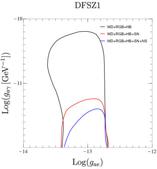
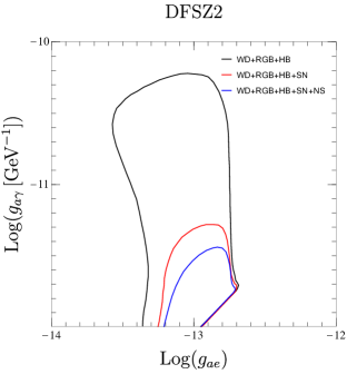
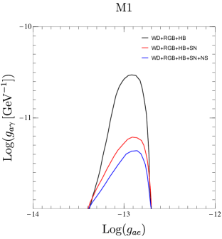
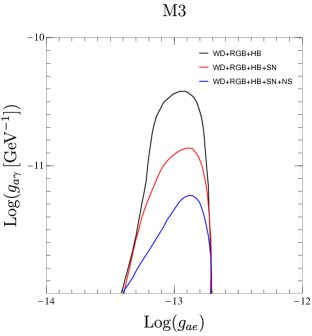
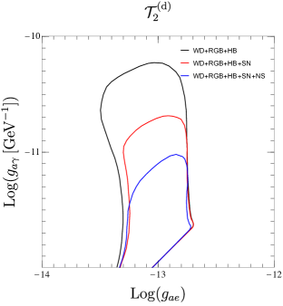
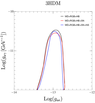
Figure 2: Contours of the $2\sigma$ regions from global fits to stellar cooling in the $g_{ae}$ vs. $g_{a\gamma}$ plane for different models. We do not show the results for models M2 and M4 that are qualitatively similar to the ones of the model M1, and the ones relative to $\mathcal{T}_{2}^{(u)}$, which strongly resemble the ones of model $\mathcal{T}_{2}^{(d)}$. Black lines correspond to the less inclusive global fit with only WD, RGB and HB data; red lines correspond to the more inclusive fit with data from SN 1987A added; blue lines are relative to the most inclusive case in which also data from NS are taken into account.

As a closing note, it is intriguing to observe that the values of the axion mass which better fit the astrophysical data reported in Table 4, fall in the range 0.2-100 meV that is suggested, in post-inflationary scenarios, by cosmological data [82].

5.2 Discovery potential of meV-scale axion experiments

In this Section we discuss the perspectives to access experimentally the parameter regions hinted by the cooling anomalies.

Fig. 2 shows that all models require a finite coupling to electrons to explain the observed stellar behavior. It is tempting, therefore, to look at experiments sensitive to the axion-electron coupling to test the preferred regions for this parameter. The most sensitive experiments of this kind are the large underground detectors XENON1T [105], LUX [106] and PandaX-II [107]. All of them can search for solar axions converted in the detector through the axio-electric effect [108]. This strategy, however, has so far allowed to probe only relatively large axion-electron couplings, in a region in tension with RGB and WD observation (see, e.g., Ref. [41]). Even the next generation of underground detectors, such as Darwin [109], will not have a sufficient sensitivity to probe the couplings favored by stellar evolution (see, e.g., Ref. [110, 111]). As we shall see, probing the axion-photon coupling offers a more efficient way to dig into the parameter region preferred by stars. Indeed, Tab. 4 shows that all our representative models give a maximal agreement with the stellar observations for axion masses in a range from a few meV to $\sim$ 100 meV, a mass range accessible to the next generation of axion helioscopes. As the name indicates, helioscopes [112] search for axions produced in the Sun. In the Sun core the main axion production channels are the Primakoff and the ABC (atomic transitions, bremsstrahlung and Compton) processes. The solar axion flux on earth is (see, e.g., Ref. [41]),

$$\frac{dN_{a}}{dt}=1.1\times 10^{39}\left[\left(\frac{g_{a\gamma}}{10^{-10}{\rm GeV}^{-1}}\right)^{2}+0.7\,\left(\frac{g_{ae}}{10^{-12}}\right)^{2}\right]\,{\rm s}^{-1}\,.$$ (5.1)

We notice that this flux gets a similar contribution from Primakoff and ABC for values of the couplings of phenomenological interest. The exact weight of the two contributions depends on the specific axion model. There are additional contributions to the solar flux induced by the axion-nucleon coupling. These are, however, normally peaked at energies too large for standard helioscopes and will be ignored here.

Helioscopes exploit a strong laboratory magnetic field to convert solar axions into X-ray photons. The conversion probability is

$$P_{a\to\gamma}=\left(\dfrac{g_{a\gamma}\,B\,L}{2}\right)^{2}\dfrac{{\rm sin}^{2}(qL/2)}{(qL/2)^{2}}\,,$$ (5.2)

where $q=q_{\gamma}-q_{a}$ is the momentum transfer provided by the magnetic field and $L$ is the length of the magnet. In vacuum, $q\simeq m_{a}^{2}/2\omega$. Coherence is ensured when $qL\ll 1$. Therefore, the helioscope sensitivity is practically mass-independent up to a certain mass threshold, $m_{\rm th}$, above which it drops rapidly. The mass threshold depends on the specific helioscope. From the above expression, we find $m_{\rm th}\approx 10\,{\rm meV}\,L_{10}^{-1/2}$, where $L_{10}$ is the magnet length in units of 10 m and we are using 3 keV as a reference solar axion energy. Whenever the coherence condition is realised, the conversion probability scales as $(g_{a\gamma}BL)^{2}$, rapidly increasing with the magnetic field and with the size of the magnet. Above $m_{\rm th}$, the sensitivity is reduced proportionally to $m_{a}^{-2}$. The sensitivity may be regained using a buffer gas in the magnet beam pipes [115]. In this case the momentum transfer is $q\simeq(m_{a}^{2}-m_{\gamma}^{2})/2\omega$. Tuning the effective photon mass, $m_{\gamma}$, to the axion mass allows to effectively regain coherence.

Below, we present a detailed study of the potential of the next generation of axion helioscopes to probe, in the regions of astrophysical interest, the various models that we have been discussing. In particular, we consider the proposed International Axion Observatory (IAXO) [116, 117, 118, 119], and its scaled versions BabyIAXO and IAXO+. Of particular interest is BabyIAXO, a scaled down (and significantly less expensive) version of IAXO, which will likely start operations in the mid of the current decade at the Deutsches Elektronen-Synchrotron (DESY) [120, 121]. The beginning of operations for IAXO are presently not known. However, even this larger helioscope does not present particular technical challenges, besides better components [119] and may become operational in a not so distant future.

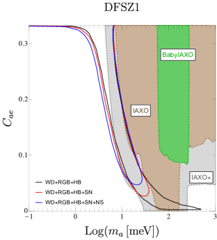
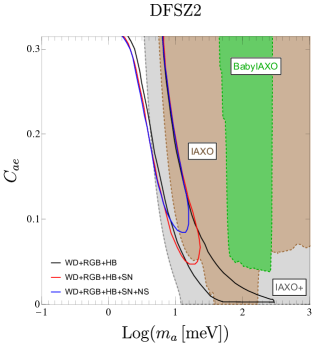
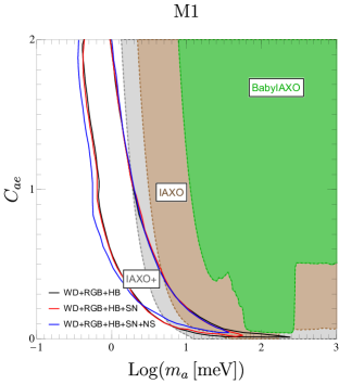
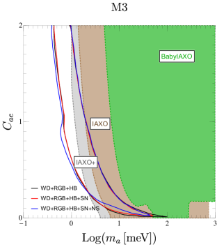
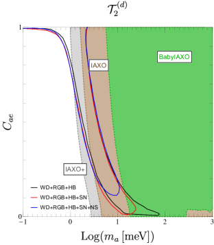
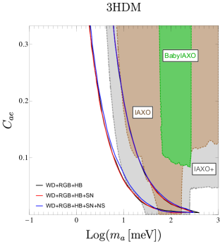
Figure 3: Contours of the $2\sigma$ regions from global fits to stellar cooling in the $m_{a}$ vs. $C_{ae}$ plane for different models, following the colour scheme defined under Fig. 2 (continuous lines). The colored regions show the helioscope sensitivities of BabyIAXO (in green), IAXO (in brown) and IAXO+ (in gray).

Finally, IAXO+ represents a more aggressive version of the IAXO helioscope, with a larger magnet and better optics. The instrumental characteristics used in this work are extracted from Ref. [119].

The helioscope potential to detect the axion models discussed in the text is shown in the six panels of Fig. 3. In all cases, we show also the regions preferred by stellar evolution, making different assumptions for the astrophysical observables. The areas corresponding to the analysis of WDs, RGB and the $R$ parameter (black contours) are the most solid, since the physics of these stars is relatively well known. The regions drawn by including also SN 1987A and data from various NS, for which the physics of axion emission is still not completely understood, are shown with separate curves (red and blue contours respectively).

In all models, the preferred parameter region appears as a relatively narrow mass band, spanning from a few meV for large electron couplings, to a few 10 meV in the opposite limit. The strong dependence of the mass boundaries on the axion-electron coupling should be clear from our previous discussion: as argued in Sec. 3.7 (see, in particular, Fig. 1) increasing the axion-electron coupling requires a smaller axion-photon coupling (and thus a smaller mass) to preserve the consistency with the observations. The axion-coupling with nucleons comes into the game when the SN or the SN+NS observables are also included. In the case of nucleo-phobic models their role is obviously reduced. In general, however, they play a more important role at low values of the axion-electron coupling, when the weight of WD and RGB data is decreased.

It is clear from the figures that the helioscopes may have a chance to detect the high mass end of the region favoured by stellar evolution. Not surprisingly, the models most accessible to the helioscopes are those with a large coupling to photons, particularly $\mathcal{T}_{2}^{(u,d)}$ (cf. Table 3). However, in general, the helioscope sensitivity increases (covering smaller masses) when the axion coupling to electrons increases, since this guarantees a larger solar flux through the ABC production processes. This feature is discernible for all the models.

A rather interesting outcome of our analysis is the potential to explore the astrophysically interesting regions of the axion parameter space for some models, and in particular for $\mathcal{T}_{2}^{(u,d)}$, already with BabyIAXO. The upgraded versions, IAXO and especially IAXO+, will be clearly able to explore much larger sections of the parameter space.

Besides helioscopes, other experiments may also probe these regions of the axion parameter space. Normally, however, such experiments rely on a set of additional assumptions, for example that axions are a substantial fraction of the local DM density. In this case, preliminary studies [122, 123] show that a new generation of haloscope detectors, based on Axionic Topological Antiferromagnets, might have the potential to explore the mass region of a few meV ($\lesssim 10\,$meV), possibly down to the axion photon couplings expected in some realistic axion models (cf. Fig. 23 in Ref. [123]). Another experiment with the potential to probe the axion mass up to several meV is ARIADNE [124]. This is a long range force experiment, which relies on the axion coupling to nucleons. The experiment sensitivity, however, depends on the CP-violating axion-scalar coupling, whose phenomenologically allowed value spans several orders of magnitude [125, 126, 127]. Assuming the maximal experimentally allowed CP-violation beyond the SM, ARIADNE could potentially probe the DFSZ axion up to masses of several meV (cf. also Fig. 2 in Ref. [10]).

6 Summary and conclusions

In this paper we have revisited the global analysis of the stellar observations in relation to the axion couplings to the SM fields, providing an update with respect to Ref. [10] that includes the most recent observational results, and enlarging considerably the collection of axion models that are confronted with the data. The set of observations used in the present work is discussed in Sec. 3 while the statistical methodology is described in Sec. 5.1. As regards the observational information, the most significant update has been the inclusion of two recent analyses of the RGB bound on the axion-electron coupling, Refs. [14, 13]. These two studies have revised the previous bound and have refined the analysis taking advantage of the new Gaia Data Release 2 [128], which has significantly improved over the previous knowledge of the distance determinations. Furthermore, we have also included new analyses of the SN [15] and NS [17] bounds on the axion-nucleon couplings.

Our study confirms a preference for non-vanishing axion couplings to electrons and photons (cf. Fig. 1). The hint is particularly strong for the axion-electron coupling, for which the best fit value lies away from zero with a significance of about $\sim 3\,\sigma$. Our best fit values for the axion-electron and axion-photon couplings are $g_{ae}\simeq 1.2\times 10^{-13}$, $g_{a\gamma}\simeq 1.8\times 10^{-11}\,{\rm GeV^{-1}}$, which are in good agreement with previous results, although, because of the new RGB analyses, the $g_{ae}$ best fit point is slightly shifted to a lower value.

To investigate the theoretical implications of these hints, we have studied a set of well motivated QCD axion models whose relevant features have been summarised in Sec. 4. On top of the two benchmark DFSZ axion models, we have considered a general class of non-universal DFSZ-like models, featuring generation-dependent PQ charges. The logic behind the models’ selection was to have in first place a sizeable $C_{ae}/C_{a\gamma}$ ratio, a favorable condition that was highlighted by the model-independent fit in Fig. 1, and next to allow for the possibility of suppressing sufficiently the axion-nucleon couplings. This latter condition allows to circumvent to some extent the strong bounds from SN 1987A and from NS. The results of our analysis for the different models are presented in Fig. 3. The qualitative feature is the same for all models: for large electron couplings, the axion photon coupling is pushed towards relatively small values (cf. Fig 1), and correspondingly the preferred region for the axion mass is also driven to relatively small values $m_{a}\sim 1\,$meV. In the case of small axion-electron coupling, on the other hand, there is a preference for a more sizeable axion-photon coupling and thus for a larger axion mass, up to 100 meV or so, depending on the model. In all cases, the inclusion of constraints on the axion-nucleon couplings from SN 1987A or from the SN and the NS pushes the mass to lower values, since these observations prefer a vanishing axion-nucleon coupling (and hence a large value of the axion decay constant $f_{a}$ which suppresses the axion mass). In the case of nucleo-phobic models however, axion-nucleon decoupling is assisted by a conspiracy between the values of the PQ charges of the quarks, and accordingly the mass suppression effect is considerably less important.

An important outcome of our study is that star evolution observations indicate a clear preference for an axion mass in the meV region, a range that is at least partially accessible to the next generation of axion helioscopes. The discovery potential of helioscopes is quite sensitive to the axion-photon coupling, which is largest in the $\mathcal{T}_{2}^{(u,d)}$ models (the complete list of axion-photon couplings for all non-universal DFSZ axion models with two Higgs doublets is given in Tab. 5). It is quite remarkable that already BabyIAXO will be able to probe some of these models, and that IAXO and IAXO+ will have a chance to cover the hinted region entirely.

It should be also stressed that a direct exploration of this region of parameter space with dedicated axion experiments will have an impact not only for axion physics but also for astrophysics. Although the stellar hints individually do not have a large significance, they all show a preference for an increased efficiency in star energy loss. Assuming no new physics is at play, this would signal a systematic problem in our understanding of stellar cooling, a possibility that would gain strength if some preferred particle physics explanations could be ruled out. Certainly, the improvements in the astrophysical instrumentation expected in the next decade or so will have a strong impact for clarifying some of these issues, and it might eventually strengthen the case for new energy loss channels. In such scenario, a new physics solution, perhaps in the form of axions, would be a most exciting result. In any case, whether this problem requires new physics, or is just a matter of understanding better the details of star evolution, or is merely an instrument calibration issue, will be clarified in the (hopefully) near future. In the meanwhile, we keep being fascinated by the synergy between astrophysics and particle physics, and by the possibility that the first evidences for the need of new particle physics could eventually come from new careful observations of the sky.

Appendix A $E/N$ factors in non-universal DFSZ models

In this Appendix we work out the discrete set of $E/N$ values that can be obtained in the most general non-universal DFSZ axion model with two Higgs doublets.

Requiring that the determinants of the mass matrices of the quarks does not vanish yields a relation between the QCD anomaly and the charges $\mathcal{X}_{ij}$ of the Higgs doublets. Denote as $H_{il}$, with charge $\mathcal{X}_{il}$, the Higgs coupled to the ($il$) entry of the mass matrix. Let us take $\mbox{det}\,M=\epsilon_{ijk}\epsilon_{lmn}\,M_{il}\,M_{jm}\,M_{kn}\neq 0$. This means that at least one term in the sum must be different from zero. Take for example $M_{il}M_{jm}M_{kn}\neq 0$. In terms of charges this means (e.g. for up-type quarks) $-\mathcal{X}_{q_{i}}+\mathcal{X}_{u_{l}}+\mathcal{X}_{il}=0$ and other two similar relations for ($jm$) and ($kn$). Since no pair of indices can be equal in the two triplets $(i,j,k)$ and $(l,m,n)$, from the non-vanishing product of the three matrix elements it follows

$$\sum_{i=1}^{3}\mathcal{X}_{q_{i}}-\sum_{i=1}^{3}\mathcal{X}_{u_{i}}=\mathcal{X}_{il}+\mathcal{X}_{jm}+\mathcal{X}_{kn}\quad\to\quad 3\mathcal{X}_{1},\ \ \mathrm{or}\ \ 2\mathcal{X}_{1}+\mathcal{X}_{2}\,,$$ (A.1)

where in the last step we assumed only two Higgs doublets, and we have defined as $H_{1}$ the doublet that occurs more times in the product of the three mass matrix entries of the non-vanishing term of the determinant. Doing the same for the down-type quarks and leptons is straightforward. However, now we have to keep the distinct possibilities for $\mathcal{X}_{1}\leftrightarrow\mathcal{X}_{2}$. So in the two Higgs doublet case we get

$$\sum_{i=1}^{3}\mathcal{X}_{q_{i}}-\sum_{i=1}^{3}\mathcal{X}_{d_{i}}=-3\mathcal{X}_{1}\,,\ \ \mathrm{or}\ \ -2\mathcal{X}_{1}-\mathcal{X}_{2}\,,\ \ \mathrm{or}\ \ -\mathcal{X}_{1}-2\mathcal{X}_{2}\,,\ \ \mathrm{or}\ \ -3\mathcal{X}_{2}\,.$$ (A.2)

Considering together Eq. (A.1) and Eq. (A.2) we see that we have $2\times 4$ different possibility for the QCD anomaly (some will give the same result). For the numerator of the second term of our $E/N$ expression, that reads $\sum_{i}\mathcal{X}_{q_{i}}-\sum_{i}\mathcal{X}_{u_{i}}+\sum_{i}\mathcal{X}_{\ell_{i}}-\sum_{i}\mathcal{X}_{e_{i}}$, one gets the same $2\times 4$ possibilities, since Eq. (A.2) holds also for the leptons. Then, by combining in all the ways the possible numerators and denominators, one gets

$$\dfrac{E}{N} =2N_{c}\,q^{2}_{d}+2q^{2}_{e}\,\dfrac{\sum_{i}\left({\cal X}_{u_{i}}-{\cal X}_{e_{i}}\right)}{\sum_{j}\left({\cal X}_{u_{i}}-{\cal X}_{d_{j}}\right)}=\dfrac{2}{3}+2(\pm 2,\pm 1,\pm\dfrac{1}{2},0,\dfrac{1}{3},\dfrac{2}{3},\dfrac{3}{2},3)\,,$$ (A.3)

corresponding to the results displayed in Table 5.

$E/N$	$|C_{a\gamma}|$	Models
$-10/3$	$5.25$	$\mathcal{T}_{2}^{(u)}$
$20/3$	$4.75$	$\mathcal{T}_{2}^{(d)}$
$-4/3$	$3.25$	M3
$14/3$	$2.75$	M4
$-1/3$	$2.25$	-
$11/3$	$1.75$	-
$2/3$	$1.25$	M1
$8/3$	$0.75$	M2
$4/3$	$0.59$	-
$5/3$	$0.25$	-
$2$	$0.08$	-

Table 5: List of all the possible values of $E/N$ in DFSZ-like models with two Higgs doublets, ordered by larger contribution to $g_{a\gamma}$. The canonical $E/N$ values for DFSZ1 and DFSZ2 coincide with those for M2 and M1, respectively.

References

- [1] R.D. Peccei and H.R. Quinn, CP Conservation in the Presence of Instantons, Phys. Rev. Lett. 38 (1977) 1440.
- [2] R.D. Peccei and H.R. Quinn, Constraints Imposed by CP Conservation in the Presence of Instantons, Phys. Rev. D16 (1977) 1791.
- [3] S. Weinberg, A New Light Boson?, Phys. Rev. Lett. 40 (1978) 223.
- [4] F. Wilczek, Problem of Strong p and t Invariance in the Presence of Instantons, Phys. Rev. Lett. 40 (1978) 279.
- [5] L. Abbott and P. Sikivie, A Cosmological Bound on the Invisible Axion, Phys. Lett. B 120 (1983) 133.
- [6] M. Dine and W. Fischler, The Not So Harmless Axion, Phys. Lett. B 120 (1983) 137.
- [7] J. Preskill, M.B. Wise and F. Wilczek, Cosmology of the Invisible Axion, Phys. Lett. B 120 (1983) 127.
- [8] M. Davier, Searches for New Particles, in Proceedings, 23RD International Conference on High Energy Physics, JULY 16-23, 1986, Berkeley, CA, 1986.
- [9] G. Raffelt, Stars as laboratories for fundamental physics: The astrophysics of neutrinos, axions, and other weakly interacting particles (5, 1996).
- [10] M. Giannotti, I.G. Irastorza, J. Redondo, A. Ringwald and K. Saikawa, Stellar Recipes for Axion Hunters, JCAP 1710 (2017) 010 [1708.02111].
- [11] K. Saikawa and T.T. Yanagida, Stellar cooling anomalies and variant axion models, JCAP 03 (2020) 007 [1907.07662].
- [12] M. Giannotti, ALP hints from cooling anomalies, in 11th Patras Workshop on Axions, WIMPs and WISPs, pp. 26–30, 2015, DOI [1508.07576].
- [13] O. Straniero, C. Pallanca, E. Dalessandro, I. Dominguez, F. Ferraro, M. Giannotti et al., The RGB tip of galactic globular clusters and the revision of the bound of the axion-electron coupling, 2010.03833.
- [14] F. Capozzi and G. Raffelt, Axion and neutrino red-giant bounds updated with geometric distance determinations, 2007.03694.
- [15] P. Carenza, T. Fischer, M. Giannotti, G. Guo, G. Martinez-Pinedo and A. Mirizzi, Improved axion emissivity from a supernova via nucleon-nucleon bremsstrahlung, JCAP 1910 (2019) 016 [1906.11844].
- [16] K. Hamaguchi, N. Nagata, K. Yanagi and J. Zheng, Limit on the Axion Decay Constant from the Cooling Neutron Star in Cassiopeia A, Phys. Rev. D 98 (2018) 103015 [1806.07151].
- [17] M.V. Beznogov, E. Rrapaj, D. Page and S. Reddy, Constraints on Axion-like Particles and Nucleon Pairing in Dense Matter from the Hot Neutron Star in HESS J1731-347, Phys. Rev. C 98 (2018) 035802 [1806.07991].
- [18] A. Sedrakian, Axion cooling of neutron stars. II. Beyond hadronic axions, Phys. Rev. D 99 (2019) 043011 [1810.00190].
- [19] L.B. Leinson, Impact of axions on the Cassiopea A neutron star cooling, 2105.14745.
- [20] L. Di Luzio, F. Mescia, E. Nardi, P. Panci and R. Ziegler, Astrophobic Axions, Phys. Rev. Lett. 120 (2018) 261803 [1712.04940].
- [21] F. Björkeroth, L. Di Luzio, F. Mescia and E. Nardi, flavour symmetries as Peccei-Quinn symmetries, JHEP 02 (2019) 133 [1811.09637].
- [22] F. Björkeroth, L. Di Luzio, F. Mescia, E. Nardi, P. Panci and R. Ziegler, Axion-electron decoupling in nucleophobic axion models, Phys. Rev. D 101 (2020) 035027 [1907.06575].
- [23] G. Grilli di Cortona, E. Hardy, J. Pardo Vega and G. Villadoro, The QCD axion, precisely, JHEP 01 (2016) 034 [1511.02867].
- [24] L. Di Luzio, M. Giannotti, E. Nardi and L. Visinelli, The landscape of QCD axion models, Phys. Rept. 870 (2020) 1 [2003.01100].
- [25] M. Srednicki, Axion Couplings to Matter. 1. CP Conserving Parts, Nucl. Phys. B 260 (1985) 689.
- [26] S. Chang and K. Choi, Hadronic axion window and the big bang nucleosynthesis, Phys. Lett. B 316 (1993) 51 [hep-ph/9306216].
- [27] M. Gorghetto and G. Villadoro, Topological Susceptibility and QCD Axion Mass: QED and NNLO corrections, JHEP 03 (2019) 033 [1812.01008].
- [28] M. Giannotti, I. Irastorza, J. Redondo and A. Ringwald, Cool WISPs for stellar cooling excesses, JCAP 05 (2016) 057 [1512.08108].
- [29] S. Hoof, F. Kahlhoefer, P. Scott, C. Weniger and M. White, Axion global fits with Peccei-Quinn symmetry breaking before inflation using GAMBIT, JHEP 03 (2019) 191 [1810.07192].
- [30] P. Di Vecchia, M. Giannotti, M. Lattanzi and A. Lindner, Round Table on Axions and Axion-like Particles, PoS Confinement2018 (2019) 034 [1902.06567].
- [31] P. Agrawal et al., Feebly-Interacting Particles:FIPs 2020 Workshop Report, 2102.12143.
- [32] N. Vinyoles, A. Serenelli, F.L. Villante, S. Basu, J. Redondo and J. Isern, New axion and hidden photon constraints from a solar data global fit, JCAP 10 (2015) 015 [1501.01639].
- [33] M.M. Miller Bertolami, B.E. Melendez, L.G. Althaus and J. Isern, Revisiting the axion bounds from the Galactic white dwarf luminosity function, JCAP 10 (2014) 069 [1406.7712].
- [34] A.H. Corsico, L.G. Althaus, M.M. Miller Bertolami and S. Kepler, Pulsating white dwarfs: new insights, Astron. Astrophys. Rev. 27 (2019) 7 [1907.00115].
- [35] A. Ayala, I. Dominguez, M. Giannotti, A. Mirizzi and O. Straniero, Revisiting the bound on axion-photon coupling from Globular Clusters, Phys. Rev. Lett. 113 (2014) 191302 [1406.6053].
- [36] O. Straniero, A. Ayala, M. Giannotti, A. Mirizzi and I. Dominguez, Axion-Photon Coupling: Astrophysical Constraints, in 11th Patras Workshop on Axions, WIMPs and WISPs, pp. 77–81, 2015, DOI.
- [37] L. Leinson, Axion mass limit from observations of the neutron star in Cassiopeia A, JCAP 08 (2014) 031 [1405.6873].
- [38] O. Straniero, I. Dominguez, L. Piersanti, M. Giannotti and A. Mirizzi, The Initial Mass–Final Luminosity Relation of Type II Supernova Progenitors: Hints of New Physics?, Astrophys. J. 881 (2019) 158 [1907.06367].
- [39] A. Friedland, M. Giannotti and M. Wise, Constraining the Axion-Photon Coupling with Massive Stars, Phys. Rev. Lett. 110 (2013) 061101 [1210.1271].
- [40] G.G. Raffelt, Astrophysical methods to constrain axions and other novel particle phenomena, Phys. Rept. 198 (1990) 1.
- [41] L. Di Luzio, M. Fedele, M. Giannotti, F. Mescia and E. Nardi, Solar axions cannot explain the XENON1T excess, Phys. Rev. Lett. 125 (2020) 131804 [2006.12487].
- [42] G. Raffelt and A. Weiss, Red giant bound on the axion - electron coupling revisited, Phys. Rev. D 51 (1995) 1495 [hep-ph/9410205].
- [43] G. Lucente and P. Carenza, Supernova bound on Axion-Like Particles coupled with electrons, 2107.12393.
- [44] J. Isern, White Dwarfs as Advanced Physics Laboratories. The Axion case, in IAU Symposium 357: White Dwarfs as probes of fundamental physics and tracers of planetary, stellar & galactic evolution, 2, 2020 [2002.08069].
- [45] M.M. Miller Bertolami, Limits on the neutrino magnetic dipole moment from the luminosity function of hot white dwarfs, Astron. Astrophys. 562 (2014) A123 [1407.1404].
- [46] B.M. Hansen, H. Richer, J. Kalirai, R. Goldsbury, S. Frewen and J. Heyl, Constraining Neutrino Cooling using the Hot White Dwarf Luminosity Function in the Globular Cluster 47 Tucanae, Astrophys. J. 809 (2015) 141 [1507.05665].
- [47] J. Isern, E. Garcia-Berro, S. Torres, R. Cojocaru and S. Catalan, Axions and the luminosity function of white dwarfs: the thin and thick discs, and the halo, Mon. Not. Roy. Astron. Soc. 478 (2018) 2569 [1805.00135].
- [48] M. Drewes, J. McDonald, L. Sablon and E. Vitagliano, Neutrino Cooling Bounds on the Internal Magnetic Fields of White Dwarfs, 2109.06158.
- [49] A.H. Córsico, L.G. Althaus, M.M. Miller Bertolami, S. Kepler and E. García-Berro, Constraining the neutrino magnetic dipole moment from white dwarf pulsations, JCAP 08 (2014) 054 [1406.6034].
- [50] S.O. Kepler, D.E. Winget, Z.P. Vanderbosch, B.G. Castanheira, J.J. Hermes, K.J. Bell et al., The pulsating white dwarf g117-b15a: Still the most stable optical clock known, The Astrophysical Journal 906 (2020) 7.
- [51] N. Viaux, M. Catelan, P.B. Stetson, G. Raffelt, J. Redondo, A.A.R. Valcarce et al., Neutrino and axion bounds from the globular cluster M5 (NGC 5904), Phys. Rev. Lett. 111 (2013) 231301 [1311.1669].
- [52] G.G. Raffelt, ASTROPHYSICAL AXION BOUNDS DIMINISHED BY SCREENING EFFECTS, Phys. Rev. D 33 (1986) 897.
- [53] G.G. Raffelt and D.S. Dearborn, Bounds on Hadronic Axions From Stellar Evolution, Phys. Rev. D 36 (1987) 2211.
- [54] G. Carosi, A. Friedland, M. Giannotti, M. Pivovaroff, J. Ruz and J. Vogel, Probing the axion-photon coupling: phenomenological and experimental perspectives. A snowmass white paper, in Community Summer Study 2013: Snowmass on the Mississippi, 9, 2013 [1309.7035].
- [55] R. Kippenhahn and A. Weigert, Stellar structure and evolution, Springer-Verlag (1994), 10.1007/978-3-642-30304-3.
- [56] K.B. McQuinn, E.D. Skillman, J.J. Dalcanton, A.E. Dolphin, J. Holtzman, D.R. Weisz et al., Observational Constraints on Red and Blue Helium Burning Sequences, Astrophys. J. 740 (2011) 48 [1108.1405].
- [57] D. Page, M.V. Beznogov, I. Garibay, J.M. Lattimer, M. Prakash and H.-T. Janka, NS 1987A in SN 1987A, Astrophys. J. 898 (2020) 125 [2004.06078].
- [58] M.S. Turner, Axions from SN 1987a, Phys. Rev. Lett. 60 (1988) 1797.
- [59] A. Burrows, M.S. Turner and R. Brinkmann, Axions and SN 1987a, Phys. Rev. D 39 (1989) 1020.
- [60] G. Raffelt and D. Seckel, Bounds on Exotic Particle Interactions from SN 1987a, Phys. Rev. Lett. 60 (1988) 1793.
- [61] J.W. Brockway, E.D. Carlson and G.G. Raffelt, SN1987A gamma-ray limits on the conversion of pseudoscalars, Phys. Lett. B 383 (1996) 439 [astro-ph/9605197].
- [62] A. Payez, C. Evoli, T. Fischer, M. Giannotti, A. Mirizzi and A. Ringwald, Revisiting the SN1987A gamma-ray limit on ultralight axion-like particles, JCAP 02 (2015) 006 [1410.3747].
- [63] J. Grifols, E. Masso and R. Toldra, Gamma-rays from SN1987A due to pseudoscalar conversion, Phys. Rev. Lett. 77 (1996) 2372 [astro-ph/9606028].
- [64] L. Calibbi, D. Redigolo, R. Ziegler and J. Zupan, Looking forward to Lepton-flavor-violating ALPs, 2006.04795.
- [65] P. Carenza, B. Fore, M. Giannotti, A. Mirizzi and S. Reddy, Enhanced Supernova Axion Emission and its Implications, 2010.02943.
- [66] T. Fischer, P. Carenza, B. Fore, M. Giannotti, A. Mirizzi and S. Reddy, Observable signatures of enhanced axion emission from proto-neutron stars, 2108.13726.
- [67] M.S. Turner, Dirac neutrinos and SN1987A, Phys. Rev. D 45 (1992) 1066.
- [68] G. Raffelt and D. Seckel, A selfconsistent approach to neutral current processes in supernova cores, Phys. Rev. D 52 (1995) 1780 [astro-ph/9312019].
- [69] W. Keil, H.-T. Janka, D.N. Schramm, G. Sigl, M.S. Turner and J.R. Ellis, A Fresh look at axions and SN-1987A, Phys. Rev. D 56 (1997) 2419 [astro-ph/9612222].
- [70] B. Fore and S. Reddy, Pions in hot dense matter and their astrophysical implications, Phys. Rev. C 101 (2020) 035809 [1911.02632].
- [71] A. Burrows, M. Ressell and M.S. Turner, Axions and SN1987A: Axion trapping, Phys. Rev. D 42 (1990) 3297.
- [72] J. Keller and A. Sedrakian, Axions from cooling compact stars, Nucl. Phys. A 897 (2013) 62 [1205.6940].
- [73] A. Sedrakian, Axion cooling of neutron stars, Phys. Rev. D 93 (2016) 065044 [1512.07828].
- [74] A. Serenelli, A. Weiss, S. Cassisi, M. Salaris and A. Pietrinferni, The brightness of the red giant branch tip. Theoretical framework, a set of reference models, and predicted observables, AA 606 (2017) A33 [1706.09910].
- [75] J.E. Kim, Weak Interaction Singlet and Strong CP Invariance, Phys. Rev. Lett. 43 (1979) 103.
- [76] M.A. Shifman, A.I. Vainshtein and V.I. Zakharov, Can Confinement Ensure Natural CP Invariance of Strong Interactions?, Nucl. Phys. B166 (1980) 493.
- [77] A.R. Zhitnitsky, On Possible Suppression of the Axion Hadron Interactions. (In Russian), Sov. J. Nucl. Phys. 31 (1980) 260.
- [78] M. Dine, W. Fischler and M. Srednicki, A Simple Solution to the Strong CP Problem with a Harmless Axion, Phys. Lett. B104 (1981) 199.
- [79] M. Badziak, G.G. di Cortona, M. Tabet and R. Ziegler, Flavor-Violating Higgs Decays and Stellar Cooling Anomalies in Axion Models, 2107.09708.
- [80] M. Gorghetto, E. Hardy and G. Villadoro, More axions from strings, SciPost Phys. 10 (2021) 050 [2007.04990].
- [81] T. Hiramatsu, M. Kawasaki, T. Sekiguchi, M. Yamaguchi and J. Yokoyama, Improved estimation of radiated axions from cosmological axionic strings, Phys. Rev. D 83 (2011) 123531 [1012.5502].
- [82] S. Hoof, J. Riess and D.J.E. Marsh, Statistical Analysis of the QCD Axion Mass Window from Topological Defects, 2108.09563.
- [83] M. Buschmann, J.W. Foster and B.R. Safdi, Early-Universe Simulations of the Cosmological Axion, Phys. Rev. Lett. 124 (2020) 161103 [1906.00967].
- [84] M. Buschmann, J.W. Foster, A. Hook, A. Peterson, D.E. Willcox, W. Zhang et al., Dark Matter from Axion Strings with Adaptive Mesh Refinement, 2108.05368.
- [85] O. Wantz and E.P.S. Shellard, Axion Cosmology Revisited, Phys. Rev. D 82 (2010) 123508 [0910.1066].
- [86] G. Ballesteros, J. Redondo, A. Ringwald and C. Tamarit, Standard Model-axion-seesaw-Higgs portal inflation. Five problems of particle physics and cosmology solved in one stroke, JCAP 1708 (2017) 001 [1610.01639].
- [87] L. Darmé, L. Di Luzio, M. Giannotti and E. Nardi, Selective enhancement of the QCD axion couplings, Phys. Rev. D 103 (2021) 015034 [2010.15846].
- [88] L. Di Luzio, B. Gavela, P. Quilez and A. Ringwald, An even lighter QCD axion, JHEP 05 (2021) 184 [2102.00012].
- [89] L. Di Luzio, F. Mescia and E. Nardi, Redefining the Axion Window, Phys. Rev. Lett. 118 (2017) 031801 [1610.07593].
- [90] L. Di Luzio, F. Mescia and E. Nardi, Window for preferred axion models, Phys. Rev. D96 (2017) 075003 [1705.05370].
- [91] F. Björkeroth, L. Di Luzio, F. Mescia and E. Nardi, Covert symmetries in the neutrino mass matrix, JHEP 02 (2020) 066 [1910.00576].
- [92] F. Björkeroth, E.J. Chun and S.F. King, Flavourful Axion Phenomenology, JHEP 08 (2018) 117 [1806.00660].
- [93] L. Di Luzio, J.F. Kamenik and M. Nardecchia, Implications of perturbative unitarity for scalar di-boson resonance searches at LHC, Eur. Phys. J. C 77 (2017) 30 [1604.05746].
- [94] L. Di Luzio and M. Nardecchia, What is the scale of new physics behind the -flavour anomalies?, Eur. Phys. J. C 77 (2017) 536 [1706.01868].
- [95] L. Allwicher, L. Di Luzio, M. Fedele, F. Mescia and M. Nardecchia, What is the scale of new physics behind the muon ?, 2105.13981.
- [96] K. Choi, S.H. Im, C.B. Park and S. Yun, Minimal Flavor Violation with Axion-like Particles, JHEP 11 (2017) 070 [1708.00021].
- [97] K. Choi, S.H. Im and C.S. Shin, Recent progress in physics of axions or axion-like particles, 2012.05029.
- [98] M. Chala, G. Guedes, M. Ramos and J. Santiago, Running in the ALPs, Eur. Phys. J. C 81 (2021) 181 [2012.09017].
- [99] M. Bauer, M. Neubert, S. Renner, M. Schnubel and A. Thamm, The Low-Energy Effective Theory of Axions and ALPs, JHEP 04 (2021) 063 [2012.12272].
- [100] K. Choi, S.H. Im, H.J. Kim and H. Seong, Precision axion physics with running axion couplings, 2106.05816.
- [101] J. De Blas et al., HEPfit: a Code for the Combination of Indirect and Direct Constraints on High Energy Physics Models, 1910.14012.
- [102] A. Caldwell, D. Kollar and K. Kroninger, BAT: The Bayesian Analysis Toolkit, Comput. Phys. Commun. 180 (2009) 2197 [0808.2552].
- [103] T. Ando, Predictive bayesian model selection, American Journal of Mathematical and Management Sciences 31 (2011) 13.
- [104] A. Gelman, J. Hwang and A. Vehtari, Understanding predictive information criteria for Bayesian models, 1307.5928.
- [105] XENON collaboration, Excess electronic recoil events in XENON1T, Phys. Rev. D 102 (2020) 072004 [2006.09721].
- [106] LUX collaboration, First Searches for Axions and Axionlike Particles with the LUX Experiment, Phys. Rev. Lett. 118 (2017) 261301 [1704.02297].
- [107] PandaX collaboration, Limits on Axion Couplings from the First 80 Days of Data of the PandaX-II Experiment, Phys. Rev. Lett. 119 (2017) 181806 [1707.07921].
- [108] K. Arisaka, P. Beltrame, C. Ghag, J. Kaidi, K. Lung, A. Lyashenko et al., Expected Sensitivity to Galactic/Solar Axions and Bosonic Super-WIMPs based on the Axio-electric Effect in Liquid Xenon Dark Matter Detectors, Astropart. Phys. 44 (2013) 59 [1209.3810].
- [109] DARWIN collaboration, DARWIN: towards the ultimate dark matter detector, JCAP 11 (2016) 017 [1606.07001].
- [110] I.G. Irastorza and J. Redondo, New experimental approaches in the search for axion-like particles, Prog. Part. Nucl. Phys. 102 (2018) 89 [1801.08127].
- [111] L. Baudis, Y. Biondi, M. Galloway, F. Girard, A. Manfredini, N. McFadden et al., Design and construction of Xenoscope – a full-scale vertical demonstrator for the DARWIN observatory, JINST 16 (2021) P08052 [2105.13829].
- [112] P. Sikivie, Experimental Tests of the Invisible Axion, Phys. Rev. Lett. 51 (1983) 1415.
- [113] F.T. Avignone, R.J. Creswick, J.D. Vergados, P. Pirinen, P.C. Srivastava and J. Suhonen, Estimating the flux of the 14.4 keV solar axions, JCAP 01 (2018) 021 [1711.06979].
- [114] CAST collaboration, Search for 14.4-keV solar axions emitted in the M1-transition of Fe-57 nuclei with CAST, JCAP 12 (2009) 002 [0906.4488].
- [115] K. van Bibber, P.M. McIntyre, D.E. Morris and G.G. Raffelt, A Practical Laboratory Detector for Solar Axions, Phys. Rev. D 39 (1989) 2089.
- [116] I.G. Irastorza et al., Towards a new generation axion helioscope, JCAP 06 (2011) 013 [1103.5334].
- [117] E. Armengaud et al., Conceptual Design of the International Axion Observatory (IAXO), JINST 9 (2014) T05002 [1401.3233].
- [118] M. Giannotti, J. Ruz and J.K. Vogel, IAXO, next-generation of helioscopes, PoS ICHEP2016 (2016) 195 [1611.04652].
- [119] IAXO collaboration, Physics potential of the International Axion Observatory (IAXO), JCAP 06 (2019) 047 [1904.09155].
- [120] BabyIAXO collaboration, Conceptual Design of BabyIAXO, the intermediate stage towards the International Axion Observatory, 2010.12076.
- [121] A. Abeln et al., Axion search with BabyIAXO in view of IAXO, PoS ICHEP2020 (2021) 631 [2012.06634].
- [122] D.J.E. Marsh, K.-C. Fong, E.W. Lentz, L. Smejkal and M.N. Ali, Proposal to Detect Dark Matter using Axionic Topological Antiferromagnets, Phys. Rev. Lett. 123 (2019) 121601 [1807.08810].
- [123] J. Schütte-Engel, D.J.E. Marsh, A.J. Millar, A. Sekine, F. Chadha-Day, S. Hoof et al., Axion quasiparticles for axion dark matter detection, JCAP 08 (2021) 066 [2102.05366].
- [124] A. Arvanitaki and A.A. Geraci, Resonantly Detecting Axion-Mediated Forces with Nuclear Magnetic Resonance, Phys. Rev. Lett. 113 (2014) 161801 [1403.1290].
- [125] J.E. Moody and F. Wilczek, New macroscopic forces?, Phys. Rev. D30 (1984) 130.
- [126] H. Georgi and L. Randall, Flavor Conserving CP Violation in Invisible Axion Models, Nucl. Phys. B276 (1986) 241.
- [127] S. Bertolini, L. Di Luzio and F. Nesti, Axion-mediated forces, CP violation and left-right interactions, Phys. Rev. Lett. 126 (2021) 081801 [2006.12508].
- [128] S. Chen, H. Richer, I. Caiazzo and J. Heyl, Distances to the Globular Clusters 47 Tucanae and NGC 362 Using Gaia DR2 Parallaxes, ApJ 867 (2018) 132 [1807.07089].