1 Introduction

Predictive and acceptable models of inflation can be obtained under the assumption that the Einstein-frame kinetic terms of some inflaton scalar contains a pole. A popular example of such models is $\alpha$–attractors [1, 2, 3, 4, 5, 6]. As reviewed in section 2, these models generate predictions that depend on the order and residue of the leading pole [7, 8]. The pole in the kinetic term is usually introduced by hand, motivated from SUSY-induced hyperbolic geometry [9, 10] or modified gravity [11, 12]. However, an often overlooked way to motivate pole cosmology is through the inclusion of a vanishing conformal factor [13]. Moreover, pole inflation can occur in the presence of multiple fields, but such scenarios have not been studied to a great extent in the literature.

In section 2, we provide an overview of pole inflation, and go on to consider more general tilts in the potential. This allows us to compute inflationary predictions assuming that they do not depend on the detailed structure of the potential around the Standard Model vacuum (that is usually ignored in studies of pole inflation). We briefly discuss how reheating can be achieved in such models.

In section 3, we explore the possibility that Einstein-frame kinetic poles arise from Jordan-frame non-minimal couplings of scalars to gravity in ordinary theories with no Jordan-frame kinetic poles. Rewriting a generic theory with $N>1$ scalars in the Einstein frame, we find that kinetic terms diverge along a $(N-1)$-dimensional surfaces in field space, singularity curves. We find that a multi-field generalisation of pole inflation can arise, but only if the Jordan-frame scalar potential $V$ satisfies some non-generic condition. Under this condition, a robust attractor profile remains even in the presence of additional fields, even with the added complication of multi-field effects. In particular, even if the field space is warped, this has little effect as its curvature does not generically diverge on the singularity curves. We show that in many cases one obtains a 2nd order pole with a specific value of the residue, which implies the same predictions of Starobinsky inflation. We examine multi-field models with conic section singular surfaces.

In section 4, we show that dimension-less theories provide a quantum structure that produces pole inflation out of the origin of field space. The non-generic structure of the potential needed to obtain pole inflation is not postulated, but comes from combining general relativity with quantum mechanics. Considering the simplest model with one scalar multiplet, we classify the inflationary predictions depending on the quantum RG running of the couplings. As we have full theories that can describe the structure of the potential around the SM minimum as well, we relax the assumption that it is not relevant for pole inflation. This allows us to obtain inflationary predictions different from usual pole inflation. Small couplings universally lead to slow RG running and to (approximatively) quadratic inflation, that is excluded because the predicted tensor/scalar ratio $r\approx 0.15$ [14] is now too large. Moderate couplings add a higher order cubic term in the potential, which can reduce $r$ by an order unity factor down to an acceptable $r\approx 0.08$ [15]. Smaller values of $r$ need larger couplings and predictions tend to become model-dependent. We explore the qualitatively different fast RG runnings that arise at larger couplings in QFT. We find that a coupling that runs non-perturbative in the UV (Landau pole, section 4.2) or in the IR (confinement, section 4.3) can lead to small $r$. On the other hand, couplings that run to an interacting fixed point in the IR (section 4.4) or in the UV (section 4.5) do not lead to particularly small $r$, at least in the examined representative models.

Conclusions are given in section 5.

2 Overview of pole inflation

In the Einstein frame, fields are parametrised such that scalars have minimal coupling to gravity. Pole inflation is obtained when the Einstein-frame action of a scalar $\phi$ has the following form, with non-minimal scalar kinetic term $K_{\rm E}(\phi)$:

$$S=\int d^{4}x\sqrt{|\det g_{\rm E}|}\bigg{[}-\frac{\bar{M}_{\rm Pl}^{2}}{2}R_{\rm E}+\frac{K_{\rm E}(\phi)}{2}{(D_{\mu}\phi)(D^{\mu}\phi)}-V_{\rm E}(\phi)+\cdots\bigg{]}.$$ (1)

We here assume one scalar $\phi$ and (without loss of generality) a pole at $\phi=0$. The Lagrangian close to the pole is usually assumed to be

$$K_{\rm E}(\phi)\simeq\frac{\alpha_{p}}{|\phi|^{p}},\qquad V_{\rm E}(\phi)\simeq V_{\rm E}(0)+V^{\prime}_{\rm E}(0)\phi,$$ (2)

corresponding to the assumption that the pole in the kinetic term is not accompanied by a pole in the potential, that is approximated by a first-order Taylor expansion. We relax this assumption by assuming the slightly more general potential with a power $q$:

$$V_{\rm E}(\phi)\equiv V_{\rm E}(0)\left[1-\frac{(\beta\phi)^{q}}{q}\right].$$ (3)

Rescaling the field $\phi\to\lambda\phi$ shows that physics only depends on the combination $\alpha_{p}\beta^{p-2}$. The potential needs to have a negative gradient such that the field is pushed away from the pole, towards the Standard Model (SM) minimum not described by the approximation of eq. (2) or (3).

With one scalar only, the non-canonical factor $K$ in the kinetic term for $\phi$ can be reabsorbed by defining a canonically normalised Einstein-frame scalar $\phi_{\rm E}(\phi)$ as ${d\phi_{\rm E}}/{d\phi}=\sqrt{K}$. The region near to the pole corresponds to an infinite range of the canonical $\phi_{\rm E}$ field if $p\geq 2$,

$$\phi_{\rm E}=\begin{cases}\displaystyle\frac{2\sqrt{\alpha_{p}}|\phi|^{1-\frac{p}{2}}}{p-2}&\hbox{if }p\neq 2,\\ \displaystyle\sqrt{\alpha_{2}}\ln\left|\phi/\bar{M}_{\rm Pl}\right|&\hbox{if $p=2$}.\end{cases}$$ (4)

This leads to a stretching of the potential and, in turn, to acceptable inflation if $q$ is low enough. In the special dimension-less case $p=2$ the field range remains infinite also at large $|\phi|$.

For later reference we recall how the inflationary predictions can be computed without rewriting the action in terms of a canonical scalar. The slow-roll parameters are given by [16, 17]

$$\epsilon\equiv\frac{1}{2}\frac{\bar{M}_{\rm Pl}^{2}}{K_{\rm E}(\phi)}\frac{V^{\prime}_{\rm E}(\phi)^{2}}{V_{\rm E}(\phi)^{2}},\qquad\eta\equiv\frac{\epsilon^{\prime}(\phi)}{\epsilon(\phi)}\frac{\bar{M}_{\rm Pl}^{2}}{K_{\rm E}(\phi)}\frac{V^{\prime}_{\rm E}(\phi)}{V_{\rm E}(\phi)},$$ (5)

and the number of $e$-foldings by

$$N(\phi)=\int_{\phi_{\rm end}}^{\phi}d\phi^{\prime}\ \frac{K_{\rm E}(\phi^{\prime})}{\bar{M}_{\rm Pl}^{2}}\frac{V_{\rm E}(\phi^{\prime})}{V^{\prime}_{\rm E}(\phi^{\prime})}.$$ (6)

Inflation ends when $\epsilon(\phi_{\rm end})\approx 1$. The scalar tilt $n_{s}$, the amplitude of scalar perturbations $A_{s}$ and the tensor-to-scalar ratio $r=A_{t}/A_{s}$ are given by the standard expressions

$$n_{s}=1-2\epsilon+\eta,\qquad A_{s}=\frac{1}{24\pi^{2}}\frac{V_{\rm E}}{\bar{M}_{\rm Pl}^{4}\epsilon},\qquad r=16\epsilon$$ (7)

which are measured at about $N\approx 50-60$ $e$-folds before the end of inflation [18]

$$n_{s}=0.9649\pm 0.0042,\qquad A_{s}\approx(2.1\pm 0.06)\times 10^{-9},\qquad r\lessapprox 0.044~{}(95\%\hbox{ C.L.}).$$ (8)

Specialising to pole inflation, the number of $e$-folds close to the pole in eq. (2) becomes

$$N\simeq\frac{\alpha_{p}}{\bar{M}_{\rm Pl}^{2}\beta^{q}}\begin{cases}\displaystyle\frac{\phi^{2-p-q}-\phi_{\rm end}^{2-p-q}}{p-2+q}&\hbox{if }p+q\neq 2,\\[8.61108pt] \displaystyle\ln\frac{\phi_{\rm end}}{\phi}&\hbox{if }p+q=2.\end{cases}\qquad\hbox{where}\qquad\phi_{\rm end}\approx\left(\frac{2\alpha_{p}}{\bar{M}_{\rm Pl}^{2}\beta^{2q}}\right)^{\frac{1}{p-2+2q}}.$$ (9)

Unlike $\phi_{\rm E}$, $N$ can be large even for $p<2$, provided that $q$ is small enough, namely that the potential is flat enough. The observables expressed in terms of $N$ are (see [19, 8] for $q=1$)

$$n_{s}=1-\frac{c}{N},\qquad r=8\left[\frac{\tilde{\alpha}_{p}^{q/(p-2+2q)}}{(p-2+q)N}\right]^{c},\qquad c=\frac{p-2+2q}{p-2+q}\geq 1$$ (10)

having defined the dimension-less combination $\tilde{\alpha}_{p}\equiv\alpha_{p}\beta^{p-2}/\bar{M}_{\rm Pl}^{2}$. Notice that $n_{s}-1$ is dominated by $\eta$, as it scales with a lower power of $N$ than $\epsilon$. Data favour $p>1.5$ if $q=1$ [8]. The case $p=2$ (also known as $\alpha$-attractor [20, 21]) gives predictions for $n_{s}$ that do not depend on the parameter $q$ in the potential: $n_{s}=1-2/N$ and $r=8\tilde{\alpha}_{2}/(qN)^{2}$, compatibly with current data if $\tilde{\alpha}_{2}/q^{2}\lessapprox 20$.

These predictions arise assuming that the structure of the potential around the SM minimum negligibly affects inflation, that takes place in the region dominated by the pole. In most realisations of pole inflation, approaching the singularity corresponds to climbing up a stretched plateau, and as a result, the field moves away from the singularity, effectively ending inflation. For a potential of the form in eq. (2), the field evolves away from the pole. Graceful exit is achieved as long as the slow-roll parameter $\epsilon$ eventually surpasses unity. While the details are model-dependent, reheating can still occur generically: even if the field cannot oscillate in the shallow canonical potential, other mechanisms can contribute to the reheating of the universe, e.g. instant preheating [25] or gravitational reheating [26]. After reheating, the canonical field will roll further down the potential, asymptotically coming to a stop due to Hubble drag, or by falling in the SM vacuum. This value of the field therefore finally sets the effective value of the Planck mass.

Finally, we discuss the opposite case where the scalar slowly rolls towards the pole, because the Einstein potential $V_{\rm E}$ is lower at the pole. This case gives rise to eternal inflation, unless $V_{\rm E}$ nearly vanishes at the pole. Only in such a special case eternal inflation is avoided, since eventually $\epsilon\approx 1$. Moreover, the pole remains inaccessible, since the canonical field is stretched to infinity. Reheating can then occur as described in above, followed by the stabilisation of the Planck mass as the canonical field gradually comes to a stop down the shallow $V_{\rm E}$.

3 Multi-field pole inflation from graviton canonicalisation

We consider $N$ scalars $\phi^{i}$ with no poles in their gauge-covariant kinetic terms and non-minimal couplings to gravity

$$S=\int d^{4}x\sqrt{|\det g|}\,\bigg{[}-\frac{1}{2}f(\phi)R+\frac{K_{ij}(\phi)}{2}(D_{\mu}\phi^{i})(D^{\mu}\phi^{j})-V(\phi)+\cdots\bigg{]}.$$ (11)

As is well known, this “Jordan frame” action can be brought to the Einstein frame where the graviton action is canonical by the field redefinition $g^{\rm E}_{\mu\nu}=g_{\mu\nu}\times f/\bar{M}_{\rm Pl}^{2}$.

For $N=1$ scalar field the action acquires the form of eq. (1) with

$$K_{\rm E}=\bar{M}_{\rm Pl}^{2}\bigg{(}\frac{K_{11}}{f}+\frac{3f^{\prime 2}}{2f^{2}}\bigg{)},\qquad V_{\rm E}(\phi)=\frac{\bar{M}_{\rm Pl}^{4}V}{f^{2}},$$ (12)

where $K_{11}$ can be assumed to be 1 since a one-dimensional field space can always be canonically normalized. Assuming that $f$ is a generic function that crosses zero at some point $f(\phi_{*})=0$ (corresponding to strong gravitational interactions) with non-vanishing derivative $f^{\prime}(\phi_{*})$, eq. (12) results in a pole of order 2 at $\phi=\phi_{*}$. However in general one has $V(\phi_{*})\neq 0$, so $V_{\rm E}(\phi_{*})=\infty$. In order to have pole inflation the Einstein-frame potential must instead be finite at the pole: one needs to assume an appropriate potential $V$ that vanishes quadratically fast at the pole.

For multiple scalar fields $\phi_{i}$, $i=1,\ldots,N$, the Einstein-frame action has the form

$$S=\int d^{4}x\sqrt{|\det g_{\rm E}|}\bigg{[}-\frac{\bar{M}_{\rm Pl}^{2}}{2}R_{\rm E}+\frac{K^{\rm E}_{ij}(\phi)}{2}{(D_{\mu}\phi^{i})(D^{\mu}\phi^{j})}-V_{\rm E}(\phi)+\cdots\bigg{]}.$$ (13)

The presence of multiple scalar degrees of freedom leads to the concept of a field space, which is equipped with a positive-definite field space metric. This metric depends on the Jordan-frame metric $K_{ij}$ and non-minimal scalar coupling to gravity $f(\phi)$, and is given by [22]

$$K^{\rm E}_{ij}=\bar{M}_{\rm Pl}^{2}\left(\frac{K_{ij}}{f}+\frac{3}{2}\frac{1}{f^{2}}\frac{\partial f}{\partial\phi^{i}}\frac{\partial f}{\partial\phi^{j}}\right),$$ (14)

We will assume canonical kinetic terms in the Jordan frame, $K_{ij}=\delta_{ij}$. Even so, the metric $K^{\rm E}_{ij}$ generically describes a warped field space, $d\phi^{2}=K^{\rm E}_{ij}d\phi^{i}d\phi^{j}$.

A generic $f(\phi)$ can vanish along some surface, which we will refer to as a singularity curve. This curve is the higher-dimensional analogue of a pole. Generically the singularity curve is $N-1$ dimensional: we here assume this is the case, and discuss in section 3.4 a special case of a singularity curve with lower dimension.

Similar to the single-field case, the potential $V_{\rm E}$ along the singularity curve will be infinite unless the surface contains points where the Jordan-frame potential $V(\phi)$ vanishes quadratically fast, in which case the resulting $V_{\rm E}(\phi)=V/f^{2}$ is finite. Even then, this is not enough to get pole inflation, because scalars that parametrise the $f=0$ surface may lead to huge gradients of the $V_{\rm E}$ potential. Therefore, a non-generic condition remains necessary to get pole inflation: defining $\phi_{*}$ as a local minimum of $V(\phi)$ restricted to the surface $f=0$, one needs $V(\phi_{*})=0$.

This condition is analogous to the vanishing of the cosmological constant, $V_{\rm E}(\phi_{\rm SM})=0$. There may be a connection between the two issues. In section 4, we will present a possible rationale for $V(\phi_{*})=0$: it is satisfied at the origin of field space in dimension-less theories. Alternatively, one might conjecture that some fundamental theory needs to have $V(\phi_{*})=0$, because it means that the regions of field space $f>0$ and $f<0$ are not physically separated by an infinite potential barrier, and that masses cannot be much heavier than the field-dependent Planck scale $\sqrt{f}$.

If the above condition is satisfied, the fields that parametrise the $f=0$ surface become very heavy near to $\phi_{*}$, and pole inflation proceeds along a one-dimensional ‘valley’ in field space.

Before we examine the attractor nature of multi-field pole inflation, it is important to understand how singularity curves affect the kinetic term of the theory and the evolution of trajectories within the field space. For a single-field theory, it is easy to see how poles cannot be crossed; indeed, the field would need to have infinite energy to do so. A more geometric way to see this is by observing that the field space distance $d\phi_{\rm E}^{2}=K_{\rm E}(\phi)d\phi^{2}$ is infinite if the path of the field traverses a pole: even if the space is one-dimensional, it is not possible to normalise the field when its domain includes poles. As a result, a theory with poles is essentially a collection of multiple canonical theories that cannot communicate with each other [23].

In the case of multiple fields, the field space metric has $N(N+1)/2$ independent entries, but it does not suffice for one of these entries to go to infinity at a point to cause the singularity curve to act as a barrier for the field. Indeed, the singularity may be an artefact of the way we have parametrised the fields. For example, consider the field space line element

$$d\phi^{2}=K_{11}(\phi_{2})d\phi_{1}^{2}+\,{d\phi_{2}^{2}}$$ (15)

It is indeed possible to cross the singularity curve $K_{11}(\phi_{2})=\infty$ if throughout the entirety of the trajectory, $d\phi_{1}=0$ is satisfied. Therefore, this is only an apparent singularity. However, compare this with the line element of a different field-space metric:

$$d\phi^{2}=K_{11}(\phi_{1})d\phi_{1}^{2}+\,{d\phi_{2}^{2}}$$ (16)

In this case, it is not possible to cross the singularity $K_{11}(\phi_{1})=\infty$ while maintaining $d\phi_{1}=0$, which indicates that this curve can never be crossed. It is worth noting that if the source of the pole is from a vanishing non-minimal coupling, the resulting singularity curve cannot be crossed. This can be seen by examining the line element: one can, at least locally, rewrite the field-space metric switching to one coordinate $\phi_{1}$ ‘perpendicular’ to the $f=0$ surface (for example $\phi_{1}=f$ itself) plus $n-1$ coordinates along which $f$ is constant. Crossing $f=0$ needs varying $\phi_{1}$, but its metric element has a pole at $f=0$. Whenever $f$ is approximatively linear around $f=0$, a dominant 2nd-order pole with residue $\tilde{\alpha}_{2}=3/2$ arises from the second term in eq. (14)

$$K_{11}^{\rm E}(\phi_{1})=\frac{3\bar{M}_{\rm Pl}^{2}}{2\phi_{1}^{2}}.$$ (17)

Let us next discuss the implications for inflation. Since the components of $K_{ij}^{\rm E}$ diverge at $f=0$, one might worry that the field-space curvature too can diverge at $f=0$. General arguments or explicit computations show that this is generically not the case. Let us consider, for example, a Jordan-frame action of the form in eq. (11) with two scalars $\phi_{1},\phi_{2}$ and coupling to gravity $f=M^{2}+\xi_{1}\phi_{1}^{2}+\xi_{2}\phi_{2}^{2}$. The field space metric is

$$K^{\rm E}_{ij}=\frac{\bar{M}_{\rm Pl}^{2}}{f^{2}}\begin{pmatrix}M^{2}+\xi_{1}(1+6\xi_{1})\phi_{1}^{2}+\xi_{2}\phi_{2}^{2}&6\bar{M}_{\rm Pl}^{2}\xi_{1}\xi_{2}\phi_{1}\phi_{2}\\ 6\bar{M}_{\rm Pl}^{2}\xi_{1}\xi_{2}\phi_{1}\phi_{2}&M^{2}+\xi_{1}\phi_{1}^{2}+\xi_{2}(1+6\xi_{2})\phi_{2}^{2}\\ \end{pmatrix}.$$ (19)

The curvature in field space diverges at $M^{2}+\xi_{1}(1+6\xi_{1})\phi_{1}^{2}+\xi_{2}(1+6\xi_{2})\phi_{2}^{2}=0$, away from $f=0$. Then, multi-field pole inflation does not significantly alter the nature of single-field pole inflation. To illustrate this, consider a simple theory with field space metric given in eq. (16). As discussed above, every theory with a $n-1$-dimensional singularity curve can be cast in this form locally by a judicious choice of coordinate system. In view of our assumptions on the potential, and since field-space curvature is finite, the inflationary trajectory has a low turn rate in field space near the pole, and therefore approaches the singularity curve with some angle $\theta$ with respect to the $\phi_{1}$-axis, as shown in fig. 1.

      

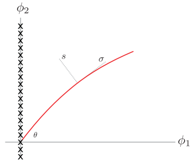
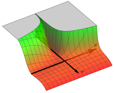
Figure 1: Left: trajectory (red line) in two-field inflation in the neighbourhood near a singularity curve (dark crosses). Right: typical pole-induced inflationary potential: a narrow flat valley in canonical coordinates.

We change the coordinate system $(\phi_{1},\phi_{2},\ldots)$ to $(\sigma,s_{1},\ldots)$, where $\sigma$ is parallel to the inflationary trajectory and acts as the effective inflaton, and $s_{i}$ are orthogonal. A dominant pole given by $K^{\rm E}_{\rm 11}(\phi_{1})=\alpha_{p}/|\phi_{1}|^{p}$, yields the following line element along the trajectory of the inflaton:

$$d\phi^{2}|_{\rm pole}=\frac{\alpha_{p}}{|\sigma|^{p}}d\sigma^{2}\,\cos^{2-p}\theta$$ (20)

having neglected sub-leading poles. The turn of the trajectory does not have an effect on the order of the pole, so the scalar tilt is unaffected. The $\cos^{2-p}\theta$ term affects the residue, and as a result can cause a suppression on the scalar-to tensor ratio, more pronounced if the trajectory is oblique to the singularity curve. The observables in eq. (10) are modified simply by making the substitution $\alpha_{p}\to\alpha_{p}\cos^{2-p}\theta$ assuming that the trajectory does not turn sharply in the direction of the singularity curve. A locally linear $f$ gives $p=2$, so that $\tilde{\alpha}_{2}=3/2$ is unaffected by the angle $\theta$, leading to the same predictions as Starobinsky inflation

$$n_{s}=1-2/N,\qquad r=12/(qN)^{2}$$ (21)

if the potential $V$ is approximatively linear, $q=1$.

Before we examine a few choice models, it is interesting to contend with the possible physical origins of singularities in the kinetic term that can lead to the behaviour described above. Kinetic poles are well established in string theory: they can be traced to Kähler potentials which arise generically due to string compactification [27, 28]. In such scenarios, additional moduli fields are not necessarily introduced. However, the fact that multiple fields contribute to inflation in our scenario (as opposed to acting like spectators) helps us draw parallels to N-flation [29]. In fact, we find ourselves in a situation similar to pole N-flation [30], where the Einstein frame kinetic term achieves a second-order ellipsoidal pole (singular locus, in our language) for an arbitrary number of fields. In both scenarios, as the fields approach the singularity, one can identify a single variable that explicitly features a pole of second order, leading to pole inflation as usual. While our treatment so far has been restricted to two fields, it is not difficult to see that near the singularity, one degree of freedom would always feature a pole, even if more fields were added. In this sense, our approach incorporates pole N-flation, albeit without reference to the physical origin of the poles themselves.

We now turn our attention to the global structure of a few particular two-field models that demonstrate the attractor nature of inflation.

3.1 Two-field pole inflation: hyperbolic singularity

We consider a model with two fields $\phi_{1}$ and $\phi_{2}$ and $f=\bar{M}_{\rm Pl}^{2}+\xi_{1}\phi_{1}^{2}+\xi_{2}\phi_{2}^{2}$ assuming $\xi_{1}=\xi_{+}>0$ and $\xi_{2}=-\xi_{-}<0$ so that there is a hyperbolic locus locus in which the kinetic term blows up. This singularity is generic: we can observe this by The field-space metric is obtained setting $M=\bar{M}_{\rm Pl}$ in eq. (19). It is convenient to switch to elliptic coordinates ($\rho,\theta$):

$$\phi_{1}=\bar{M}_{\rm Pl}\sqrt{\frac{2}{\xi_{+}}}\sinh\rho\sin(\pi/4-\theta),\qquad\phi_{2}=\bar{M}_{\rm Pl}\sqrt{\frac{2}{\xi_{-}}}\cosh\rho\cos(\pi/4-\theta)$$ (22)

so that $f=\bar{M}_{\rm Pl}^{2}\cosh(2\rho)\sin(2\theta)$, the singularity locus is $\theta=0$, and lines of constant $\theta$ are hyperbolæ. Only the $K^{\rm E}_{\theta\theta}$ component contains a 2nd-order pole, and this is the only term relevant for computing the observables:

$$K^{\rm E}_{\theta\theta}|_{\rm pole}=\frac{3\bar{M}_{\rm Pl}^{2}}{2\theta^{2}}.$$ (23)

It is important to note that the linear vanishing of the non-minimal coupling $f$ in these coordinates is not a coordinate artifact, as we can verify that at the singularity locus, the first derivative of the kinetic term with respect to the original field $\phi_{1}$ still goes to infinity:

$$K_{,\phi_{1}}|_{\rm pole}=\frac{1}{M_{P}^{2}+\xi_{+}\phi_{1}^{2}+\xi_{-}\phi_{2}^{2}}\begin{pmatrix}-24\xi_{+}^{3}\phi_{1}^{3}&24\xi_{+}^{2}\sqrt{\xi_{-}}\phi_{1}^{2}\sqrt{M_{P}^{2}+\xi_{+}\phi_{1}^{2}}\\ 24\xi_{+}^{2}\sqrt{\xi_{-}}\phi_{1}^{2}\sqrt{M_{P}^{2}+\xi_{+}\phi_{1}^{2}}&-24\xi_{+}\xi_{-}\phi_{1}\left(M_{P}^{2}+\xi_{+}\phi_{1}^{2}\right)\end{pmatrix},$$ (24)

and similarly for $K_{,\phi_{2}}$.

The poles in the field-space metric in the new elliptic coordinates is more easily obtained computing eq. (14) in the new coordinates. The Einstein frame potential is $V_{\rm E}=V\cosh^{2}\rho/{\sin^{2}2\theta}$. Pole inflation is obtained if $V$ is approximatively quadratic around the pole at $\theta=0$ and $\rho=\rho_{0}$ for (at least one) value of $\rho=\rho_{0}$. In formulæ, we need

$$V=R(\rho,\theta)\left[c_{\theta\theta}\frac{\theta^{2}}{2}+c_{\rho\rho}\frac{(\rho-\rho_{0})^{2}}{2}+c_{\theta\rho}\theta(\rho-\rho_{0})\right]$$ (25)

where $R$ is any smooth function around the pole. The $c_{ij}$ matrix determines the angle of incidence $\theta$ of the inflationary trajectory. Along it one gets a pole with order $p=2$ and residue $\tilde{\alpha}_{2}=3/2$, and thereby the inflationary predictions of eq. (21).

3.2 Two-field pole inflation: elliptic singularity

A similar model is obtained assuming $\xi_{1,2}<0$. The singularity curves are now ellipses, conveniently parametrised using stretched polar coordinates $(\rho,\theta$)

$$\phi_{1}=\frac{\bar{M}_{\rm Pl}}{\sqrt{-\xi_{1}}}\rho\sin\theta,\qquad\phi_{2}=\frac{\bar{M}_{\rm Pl}}{\sqrt{-\xi_{2}}}\rho\cos\theta,$$ (26)

so that $f=\bar{M}_{\rm Pl}^{2}(1-\rho^{2})$. The singularity curve is $\rho=1$, and we must expand around it in the $f\geq 0$ region. The potential is $V_{\rm E}=V/(1-\rho^{2})^{2}$. In polar coordinates, the only element of the kinetic matrix with a pole around $\rho=1$ is

$$K_{\rho\rho}^{\rm E}|_{\rm pole}=\frac{3\bar{M}_{\rm Pl}^{2}}{2(1-\rho)^{2}}.$$ (27)

The resultant theory has once again attractor predictions given in eq. (21), and reheating proceeds in a similar way to the previous subsection.

3.3 Two-field pole inflation: linear singularity

We next examine inflation that features no inherent scale. Such a model will be further motivated in section 4. In this case, we assume $f=\xi_{1}\phi_{1}^{2}+\xi_{2}\phi_{2}^{2}$ with $\xi_{1}=\xi_{+}>0$ and $\xi_{2}=-\xi_{-}<0$. The field-space curvature diverges at $\xi_{1}(1+6\xi_{1})\phi_{1}^{2}+\xi_{2}(1+6\xi_{2})\phi_{2}^{2}=0$, away from the singularity curves, that are the two crossed lines $\phi_{1}/\phi_{2}=\pm\,\sqrt{\xi_{-}/\xi_{+}}$. The best way to parametrise this theory is therefore a skew coordinate system

$$\phi_{\pm}=\phi_{1}\sqrt{\xi_{+}}\pm\phi_{2}\sqrt{\xi_{-}}$$ (28)

so that $f=\phi_{+}\phi_{-}$ and the two singularity curves are $\phi_{+}=0$ and $\phi_{-}=0$. Due to the symmetry of the situation, we can focus on $\phi_{-}=0$. This once again gives

$$K^{\rm E}_{++}|_{\rm pole}=\frac{3\bar{M}_{\rm Pl}^{2}}{2\phi_{-}^{2}}.$$ (29)

The resultant theory once again gives the attractor predictions of eq. (21). As such, it is enough for the potential to vanish on at least one point on the singularity curve. A potential with this property and which is exactly scale-invariant (quartic in the fields) vanishes along all the singularity curve

$$V=\frac{\lambda}{4}\left(\xi_{1}\phi_{1}^{2}+\xi_{2}\phi_{2}^{2}\right)^{2}.$$ (30)

3.4 Point singularity

We finally examine the situation where $f$ is not linear around the pole and/or the singularity curve along which $f=0$ has less than $N-1$ dimensions.

We consider a scale-invariant theory with one field $\phi$ (see also [Cooper:1981byv]), so that

$$V(\phi)=\lambda\frac{\phi^{4}}{4},\qquad f(\phi)=\xi\phi^{2}$$ (31)

where $\xi$ and $\lambda$ are dimension-less coupling constants. This leads to a 2nd order pole at $\phi=0$, $K_{\rm E}=\bar{M}_{\rm Pl}^{2}(1+6\xi)/\xi\phi^{2}$. The residue $\alpha_{2}/\bar{M}_{\rm Pl}^{2}=6+1/\xi$ has a non-standard value because $f$ is quadratic (rather than linear) around the pole at $\phi=0$. The Einstein-frame potential is finite and exactly flat, $V_{\rm E}=\bar{M}_{\rm Pl}^{4}\lambda/4\xi^{2}$, corresponding to $q=0$ in the language of section 2. Planck-suppressed non-renormalisable operators in the potential could nonetheless still create a tilt and the desired SM minimum.

Let us next consider $N=2$ fields and a scale-invariant $f=\xi_{1}\phi_{1}^{2}+\xi_{2}\phi_{2}^{2}$ with $\xi_{1,2}>0$. Then $f=0$ only at the point at the origin in field space, $\phi_{1}=\phi_{2}=0$. It is convenient to use stretched polar coordinates

$$\phi_{1}=\frac{\rho}{\sqrt{\xi_{1}}}\cos\theta,\qquad\phi_{2}=\frac{\rho}{\sqrt{\xi_{2}}}\sin\theta,$$ (32)

such that $f=\rho^{2}$ is not linear around the pole at $\rho=0$. The dominant pole for the inflaton field $\rho$ is again 2nd-order, and its residual has the same non-standard value

$$K_{\rho\rho}^{\rm E}=\frac{\bar{M}_{\rm Pl}^{2}(1+6\xi)}{\rho^{2}\xi}\qquad\hbox{with}\qquad\frac{1}{\xi}\equiv\frac{\cos^{2}\theta}{\xi_{1}}+\frac{\sin^{2}\theta}{\xi_{2}}$$ (33)

obtained in the effective one-field case along a trajectory with angle $\theta$. With more than $N=2$ scalars, pole inflation similarly arises from the origin of field space.

4 Pole inflation in dimension-less quantum theories

As discussed in the previous section, making gravity canonical can lead to poles in the scalar kinetic terms, but pole inflation only arises if the potential $V$ satisfies non-generic conditions. We already mentioned one possible rationale for them: as the factor $f$ corresponds to a scale transformation, nearly scale-invariant theories can have special properties. We restrict the generic theory written in the Jordan frame in eq. (11) to field theories with dimension-less couplings only.

At quantum level, quantum corrections break classical scale invariance. The quantum counterpart of eq. (31) is well approximated by the classical expressions with running couplings renormalised around the field value $\phi$

$$V(\phi)=\lambda(\phi)\frac{\phi^{4}}{4},\qquad f(\phi)=\xi(\phi)\phi^{2}.$$ (34)

$K_{\rm E}(\phi)$ is no longer a simple power, and the Einstein-frame potential

$$V_{\rm E}(\phi)=\frac{\bar{M}_{\rm Pl}^{4}}{4}\frac{\lambda(\phi)}{\xi^{2}(\phi)}$$ (35)

is no longer flat. Roughly speaking, one can now have pole inflation with $p\approx 2$ and $q\approx 0$, where the small deviations from the classical values arise from anomalous dimension. More precisely, $V_{\rm E}(\phi)$ cannot be approximated as a simple function, unlike what is assumed in general treatments of pole inflation. The reason is that RG dynamics depend on $\ln\phi\propto\phi_{\rm E}$, the canonical scalar in eq. (4).

Since details of these functions matter, in this section we consider models that describe the SM minimum too. The scalar today sits at the SM minimum, $\phi=\phi_{0}$, where $f(\phi_{0})=\bar{M}_{\rm Pl}^{2}$ and $V_{\rm E}(\phi_{0})=0$, in view of the nearly vanishing of the cosmological constant. The potential $V_{\rm E}$ features the desired SM minimum if the RG running is such that

$$\lambda(\phi_{0})=0,\qquad\beta_{\lambda}(\phi_{0})=0,\qquad\beta_{\beta_{\lambda}}(\phi_{0})>0$$ (36)

at a field value $\phi_{0}$ such that $f(\phi_{0})=\bar{M}_{\rm Pl}^{2}$ [14]. In the above equation $\beta_{x}\equiv dx/d\ln\bar{\mu}$ denotes the $\beta$ function of a generic coupling $x$, and $\beta_{\beta_{\lambda}}$ denotes the $\beta$ function of the combination of couplings that arise in $\beta_{\lambda}$, the $\beta$ function of $\lambda$. A similar notation is used below. Since $\beta_{\beta_{\lambda}}\neq 0$, the tuning of parameters implied by $\beta_{\lambda}$ cannot be explained as a fixed point.

The slow-roll parameters of eq. (5) that determine inflation predictions can be written in terms of the beta functions of the theory as

$$\epsilon =\frac{\xi}{1+6\xi}\frac{1}{2}\bigg{[}\frac{\beta_{\lambda}}{\lambda}-2\frac{\beta_{\xi}}{\xi}\bigg{]}^{2},$$ (37)

$$\eta =\frac{\xi}{1+6\xi}\bigg{[}2\frac{\beta_{\beta_{\lambda}})}{\lambda}-4\frac{\beta_{\beta_{\xi}}}{\xi}-2\frac{\beta^{2}_{\lambda}}{\lambda^{2}}+4\frac{\beta^{2}_{\xi}}{\xi^{2}}+\frac{\beta_{\xi}/\xi}{1+6\xi}\left(\frac{\beta_{\lambda}}{\lambda}-2\frac{\beta_{\xi}}{\xi}\right)\bigg{]}.$$ (38)

This shows that slow-roll inflation is generically achieved in theories with perturbative dimension-less couplings. More specifically $\epsilon,\eta\sim\lambda^{2}/(4\pi)^{4}$ contain a two loop suppression away from the potential minimum where inflation ends and $\epsilon,\eta$ become large in view of the vanishing $\lambda$ at the denominator.

Since $p=2$, beyond the pole at the origin in field space $\phi=0$, another pole exists at $\phi=\infty$, so that both small-field and large-field inflation can give acceptable predictions.

4.1 Inflation with dimension-less theories at small coupling

If couplings are so small that away from the minimum we have $|\epsilon|,|\eta|\ll 0.01$ (the size suggested by data about $n_{s}=1-2\epsilon+\eta$), only the field region around the potential minimum matters. Then the potential can be expanded in Taylor series: at leading order the inflationary potential is quadratic as function of the canonically normalised Einstein-frame scalar $\phi_{\rm E}(\phi)$, defined by ${d\phi_{\rm E}}/{d\phi}=\sqrt{K}$. This implies that $N\lessapprox 60$ $e$-folds of inflation probe about 3 orders of magnitude of RG running

$$\left|\ln\frac{\phi}{\phi_{0}}\right|\approx\sqrt{\frac{4\xi N}{1+6\xi}}\lessapprox 6$$ (39)

and that the tensor/scalar ratio is $r\simeq 8/N\approx 0.15$ [14], above current bounds. Including the next cubic order in the Taylor series can increase or reduce $r$ [15]. A substantial reduction down to acceptable values is possible; however whenever cubics have an order unity effect (allowing to reduce $r$ down to currently acceptable values $r\sim 0.08$) one expects that higher-order effects too start becoming relevant: one can no longer use the Taylor expansion and needs a full theory.

In a full theory, $r$ gets significantly reduced (below the small-coupling limit that gives quadratic inflation) if the couplings are such that the two-loop factor in eq. (37) gives the desired $|\epsilon|,|\eta|\sim 0.01$. This corresponds to mild dimension-less couplings of order one. More precisely, couplings must run by order unity in the $\approx 3$ orders of magnitudes probed by small-coupling inflation according to eq. (39).

Sizeable couplings and a fast RG running come with the danger that couplings blow up, running to strong coupling in IR (endangering computability and inflation) and/or in the UV (Landau poles presumably ruin the consistency of the theory), unless an interacting fixed point in the UV (asymptotic safety) or in the IR is dynamically reached.

In theories where a scalar $\phi$ charged under some gauge interaction has one quartic $\lambda$ and one Yukawa coupling $y$ (its presence allows to get a quantum potential with the desired SM minimum at $\phi_{0}$), the one-loop RGE have the generic form

$$\begin{array}[]{rclrcl}\displaystyle\frac{dg^{2}}{dt}&=&-bg^{4},&\displaystyle\frac{d\lambda}{dt}&=&\lambda(s_{\lambda}\lambda+s_{\lambda y}y^{2}-s_{\lambda g}g^{2})-s_{y}y^{4}+s_{g}g^{4},\\[8.61108pt] \displaystyle\frac{dy^{2}}{dt}&=&y^{2}(f_{y}y^{2}-f_{g}g^{2}),&\displaystyle\frac{d\xi}{dt}&=&\displaystyle\frac{1}{12}(1+6\xi)(\tilde{s}_{\lambda}\lambda+s_{\lambda y}y^{2}-s_{\lambda g}g^{2}),\end{array}$$ (40)

with positive and gauge-independent order one coefficients $f_{i}$ and $s_{i}$, that depend on the specific model. Notice the multiple appearance of $s_{\lambda y}$ and $s_{\lambda g}$. We defined $t=\ln(E^{2}/E_{0}^{2})/(4\pi)^{2}$ and included QFT effects and ignored quantum gravity effects (computable in agravity).

Let us count the number of free parameters:

• The SM minimum is generated if $\lambda(\phi_{0})=\beta_{\lambda}(\phi_{0})$ and $\beta_{\beta_{\lambda}(\phi_{0})}>0$: this fixes $\lambda$ and $y$ as $\lambda_{0}=0$, $y_{0}^{2}/g_{0}^{2}=\sqrt{s_{g}/s_{\lambda}}$ and restricts $f_{g}-f_{y}\sqrt{s_{g}/s_{y}}>b$ (the left side of the inequality is proportional to the sign of $\beta_{y}$ at $\phi_{0}$).

• The condition $\xi_{0}\phi_{0}^{2}=\bar{M}_{\rm Pl}^{2}$ together with the measured value of the amplitude of scalar perturbations (see eq. (7) and (8)) can be used to fix $\xi$ and $\phi_{0}$: assuming order one couplings one needs $\xi\sim 100$ and thereby sub-Planckian $\phi_{0}=\bar{M}_{\rm Pl}/\sqrt{\xi}$. Then the RG for $\xi_{0}\gg 1$ implies it undergoes a nearly-multiplicative renormalisation, with beta-function $\beta_{\xi}=(1+6\xi_{0})(-s_{\lambda g}+s_{\lambda y}\sqrt{s_{g}/s_{y}})/12$ at $\phi_{0}$ that will be negative in all computed models.

In any given model, the gauge coupling $g$ remains as the only free parameter (with small values giving quadratic inflation). However, many models are possible and give different RG coefficients.

We next discuss the possible irreversible RG flows (limit cycles are considered impossible [33, 34]): to strong coupling in the UV (section 4.2), to strong coupling in the IR (section 4.3), to an IR fixed-point (section 4.4), to an UV fixed-point (asymptotic safety, section 4.5).

      

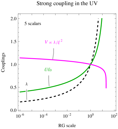
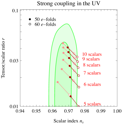
Figure 2: Inflation with a scalar quartic that becomes non-perturbative in the UV hitting a Landau pole. Left: sample of RG running in the model of section 4.2. Right: its possible inflationary predictions, assuming small-field inflation that ends at non-perturbative $\lambda=(4\pi)^{2}$ (dark red) or $10^{3}$ (light red).

4.2 Inflation with strong coupling in the UV

If one wishes to consider RG running that leads to strong coupling at high energy (and thereby to a Landau pole, possibly sub-Planckian) the simplest theory has a Higgs-like scalar: $N$ ultra-light scalar real degrees of freedom $\phi_{i}$ with maximal global symmetry $\,{\rm SO}(N)$, so that

$$f=\phi_{1}^{2}+\cdots+\phi_{N}^{2},\qquad V=\frac{\lambda}{4}(\phi_{1}^{2}+\cdots+\phi_{N}^{2})^{2}.$$ (41)

For example, the SM Higgs has $N=4$: the global symmetry arises accidentally due to the $\,{\rm SU}(2)_{L}$ gauge symmetry and the Higgs is much lighter than the Planck scale for unclear reasons. Assuming that gauge interactions are absent or negligible, the one-loop RGE of the theory are

$$(4\pi)^{2}\beta_{\lambda}=2(8+N)\lambda^{2},\qquad(4\pi)^{2}\beta_{\xi}=(1+6\xi)\frac{2+N}{3}\lambda.$$ (42)

So $\lambda$ runs to small values in the IR, and $\xi+1/6$ is multiplicatively renormalised

$$\lambda=\frac{\lambda_{0}}{1-2(8+N)t\lambda_{0}},\qquad\xi+\frac{1}{6}=(\xi_{0}+\frac{1}{6})\left(\frac{\lambda}{\lambda_{0}}\right)^{(2+N)/(8+N)}.$$ (43)

For $\xi\gg 1$, the Einstein-frame potential satisfies $V_{\rm E}=V_{\rm E}^{0}(\lambda/\lambda_{0})^{(4-N)/(8+N)}$, allowing small-field inflation for $N\geq 4$ and large-field inflation for $N<4$. In the special case $N=4$, the quantum potential is flat up to terms suppressed by $\xi$. Fig. 2a shows the running in the quasi-flat case $N=5$.

In this minimal model, inflation ends near to the Landau pole at strong coupling, where $\epsilon,\eta$ can become of order unity but the perturbative computation becomes unreliable. Up to this caveat, fig. 2b shows the resulting predictions. Like in pole inflation, we assumed small-field inflation out of the pole, and so the predictions only hold assuming that the extra physics needed to generate the SM minimum starts to be relevant after inflation end. Otherwise, the predictions would be modified depending on the extra physics near to the SM minimum. For example, one could add non-renormalisable operators, or an extra scalar, or extra couplings that appropriately modify the running. In the next sections we will pursue the latter strategy, considering less minimal models that allow for RG runnings without Landau poles.

      

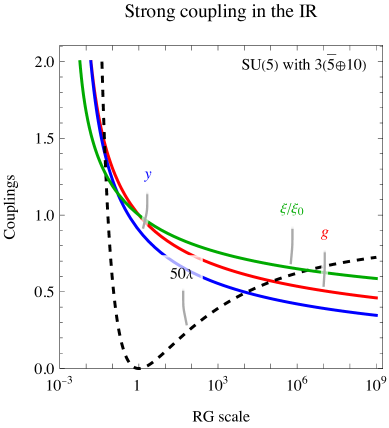
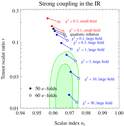
Figure 3: Inflation with couplings that become non-perturbative in the IR giving rise to confinement. Left: sample of RG running in the model of section 4.3 with $N_{f}=3$ and gauge coupling $g=1$ at the SM minimum after inflation. Right: its inflationary predictions for different values of $g$.

4.3 Inflation with strong coupling in the IR

In non-abelian gauge theories with a small matter content (loosely speaking, fewer scalars and fermions than vectors), the asymptotically free gauge coupling $g$ runs to non-perturbative values at some low-energy scale $\Lambda$, analogously to QCD. We add a charged scalar $\phi$ with a quartic coupling $\lambda$ that runs in a similar way. Ignoring the issue of generating the SM minimum, large-field inflation would end at $\phi\sim\Lambda$. We generate the SM minimum at a scale $\phi=\phi_{0}$ by adding fermions, such that one Yukawa coupling $y$ induces a running $\lambda$ with the desired SM minimum at an arbitrary scale $\phi_{0}$. If $\phi_{0}$ is many orders of magnitude above $\Lambda$, the couplings $g(\phi_{0})$ are weak and one gets the predictions of quadratic inflation. If $\phi_{0}$ is not much larger than $\Lambda$ so that couplings $g(\phi_{0})$ are moderately large, one gets different predictions.

As a concrete example, we consider a theory similar to the $\,{\rm SU}(5)$ extension of the SM: a $\,{\rm SU}(5)$ gauge theory with $N_{f}$ generations of chiral Weyl fermions in the anomaly-free $\bar{5}\oplus 10$ representation and a complex scalar $\Phi$ in the fundamental 5 with quartic $\lambda|\Phi|^{4}$ and Yukawa coupling $y\,\Phi\,10\,10$. With this coupling, order one factors in the RG equations

$$\begin{array}[]{ll}\displaystyle(4\pi)^{2}\beta_{g}=-(\frac{109}{6}+\frac{2}{3}N_{f})g^{3},&\displaystyle(4\pi)^{2}\beta_{\lambda}=12\lambda(3\lambda+y^{2}-\frac{12}{5}g^{2})-6y^{4}+\frac{99}{25}g^{4},\\[4.30554pt] \displaystyle(4\pi)^{2}\beta_{y}=y(6y^{2}-\frac{108}{5}g^{2}),&\displaystyle(4\pi)^{2}\beta_{\xi}=(1+6\xi)(4\lambda+y^{2}-\frac{12}{5}g^{2}).\end{array}$$ (44)

allow, if $N_{f}>1$, to generate the desired minimum in the Coleman-Weinberg $\Phi$ potential with a small enough Yukawa coupling (unfavourable order one factors would lead to a Landau pole in $y$ and/or to no minimum). Fig. 3a shows a sample of RG running, with $y$ and $\lambda$ tuned in such a way that the Einstein potential has the desired SM minimum.

As expected, for small couplings both small-field and large-field inflation reproduce the predictions of quadratic inflation, with its too large $r\approx 0.15$.

Small-field inflation (from low energies $\phi<\phi_{0}$, in red in fig. 3b) leads to an excluded tensor/scalar ratio $r$, because larger than the quadratic limit. This is due to the larger value of the gauge coupling at low energies, and it is partially counter-acted by the fact that $\xi$ runs to larger values at lower energies.

The opposite happens for large-field inflation (from high energies $\phi>\phi_{0}$, in blue in fig. 3b). Since couplings run to smaller values at higher energy, a substantial reduction in $r$ needs a $\phi_{0}$ not much above $\Lambda$. Different models would give qualitatively similar predictions (see for example fig. 3 of [15]).

4.4 Inflation with an IR fixed-point

Non-Abelian gauge theories with a large enough matter content exhibit a qualitatively different behaviour: the gauge coupling $g$ runs in the infra-red to a fixed-point $g=g_{*}$. Banks and Zaks [35] showed that this phenomenon can be computed perturbatively in theories with matter content such that the one-loop RG coefficient $-b$ is negative and accidentally small, and its two-loop counterpart $b^{\prime}$ is positive. Then the 2 loop term in the RGE for $g$ is relevant,

$$\frac{dg^{2}}{dt}=-bg^{4}+\frac{b^{\prime}}{(4\pi)^{2}}g^{6}+\cdots,\qquad t=\frac{\ln\mu^{2}/\mu_{*}^{2}}{(4\pi)^{2}}$$ (45)

while higher order terms can be neglected, so that the IR fixed-point $g^{2}_{*}=(4\pi)^{2}b/b^{\prime}$ is reliably computed. The analytic solution to RGE where the fixed-point is approached for $\mu\lessapprox\mu_{*}$ is

$$bt=\frac{1}{g^{2}}+\frac{1}{g_{*}^{2}}\ln\left(\frac{g_{*}^{2}}{g^{2}}-1\right)\qquad\hbox{i.e.}\qquad g^{2}=\frac{g_{*}^{2}}{1+W(e^{-1+bg_{*}^{2}t})}$$ (46)

having introduced the Lambert function $W(z)e^{W(z)}=z$ to invert the relation between $g$ and $t$. When $g$ reaches its IR fixed-point, the Yukawa $y$ and quartic coupling $\lambda$ behave as follows:

• $y$ too reaches an IR fixed-point, $y_{*}^{2}/g_{*}^{2}=f_{g}/f_{y}$.

• If the condition $\beta_{\lambda}=0$ is satisfied at two values real of $\lambda$ (this depends on the values of the RG coefficients), the higher solution is an IR-attractive fixed-point for $\lambda$. If it is positive, the potential is acceptable. In other words, dynamics self-adjusts the dimension of the $\phi^{4}$ composite operator to its classical dimension. The fact that $\lambda(\bar{\mu})$ remains finite at low energy means that our pole-inflation assumption $V(0)=0$ is satisfied.

        

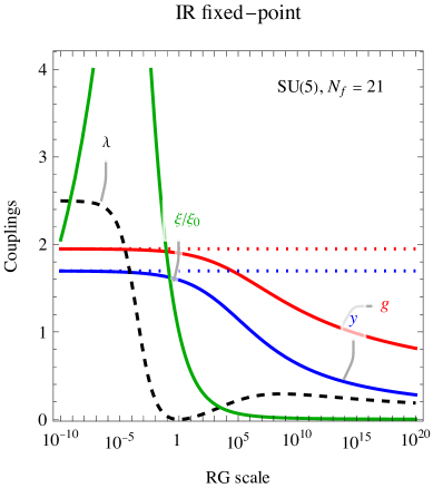
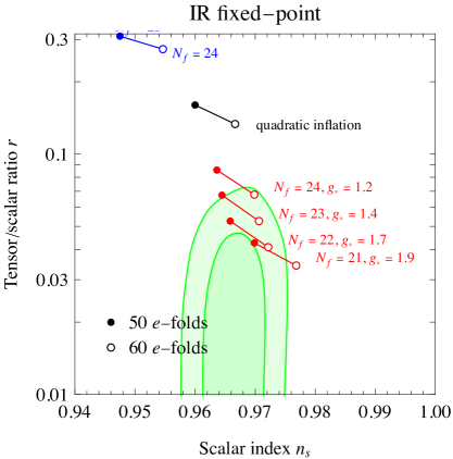
  Figure 4: Inflation with couplings that approach a fixed point in the IR. Left: sample of RG running in the model of section 4.4 for $N_{f}=21$ corresponding to IR fixed-point $g_{*}\approx 1.9$. Right: its small-field (red) and large-field (blue) inflationary predictions for different values of $N_{f}$.

• At the fixed-point for $\lambda,y$, the $\xi$ coupling gets renormalised multiplicatively. In other words, the $\phi^{2}$ composite operator acquires an anomalous dimension.

We consider, as a simple example, a $\,{\rm SU}(N)$ gauge theory with $N_{f}$ Weyl fermions $\psi_{i}\oplus\psi^{c}_{i}$ in the $N\oplus\bar{N}$, one fermion singlet $\nu$, one complex scalar $\Phi$ in the fundamental $N$. Without loss of generality, the Yukawa interactions and the potential can be written as

$$\mathscr{L}_{\rm Yuk}=y\,\Phi\psi_{1}^{c}\nu+\bar{y}\,\Phi^{*}\psi_{1}\nu+\hbox{h.c.},\qquad V=\lambda|\Phi|^{4}.$$ (47)

The RG equations are

$$\frac{dg^{2}}{dt} =-bg^{4}+\frac{1}{(4\pi)^{2}}\left[\frac{\left(\left(13N^{2}-3\right)N_{f}-34N^{3}+4N^{2}-3\right)}{3N}g^{6}-\frac{1}{2}g^{4}\left(\bar{y}^{2}+y^{2}\right)\right],$$ (48)

$$\frac{dy^{2}}{dt} =y^{2}\left[\frac{3+N}{2}y^{2}+\frac{6+N}{2}-\frac{3(N^{2}-1)}{2N}g^{2}\right],\hskip 100.00015pt$$ (49)

$$\frac{d\lambda}{dt} =\lambda\left[2\lambda(N+4)+2(y^{2}+\bar{y}^{2})+3\tfrac{N^{2}-1}{N}g^{2}\right]-(y^{2}+\bar{y}^{2})^{2}+3g^{4}\tfrac{N\left(N^{2}+N-4\right)+2}{8N^{2}},$$ (50)

$$\frac{d\xi}{dt} =(6\xi+1)\left[\frac{1}{6}\left(\bar{y}^{2}+y^{2}\right)-\frac{N^{2}-1}{4N}g^{2}+\frac{N+1}{3}\lambda\right],$$ (51)

where $b=\frac{11}{3}N-\frac{2}{3}N_{f}-\frac{1}{6}$ is chosen small and positive, and a similar RG holds for $\bar{y}$. The perturbative IR fixed point for $g$ exists for $N_{f}\approx 11N/2$; it is lost for higher $N_{f}$ and perturbative control is lost for lower $N_{f}$ (we are interested in mildly large couplings). Given the order one factors, the acceptable parameter space of the model is somehow restricted. Assuming, for simplicity, $\bar{y}=y$, the value of the Yukawa coupling $y$ needed to have the desired SM minimum in the SM minimum obtained imposing $\lambda=\beta_{\lambda}=0$ is below the fixed-point value of $y$ for $3<N<12$ by less than $4\%$ (larger values of $y$ lead to a Landau pole). Furthermore, the gauge coupling $g$ at the SM minimum where $\lambda=\beta_{\lambda}=0$ must be similarly near to its fixed point to avoid having maximum rather than a minimum, as can be seen by imposing $\beta_{\beta_{\lambda}}>0$.

Fig. 4a shows a sample of RG running assuming $N=5$ colours and $N_{f}=21$ flavours. We choose a somehow low $N_{f}$ such that the Banks-Zaks fixed-point has a moderately large coupling $g_{*}$, in order to obtain inflationary predictions that substantially deviate from those of quadratic inflation obtained in the weak coupling limit. Fig. 4b shows that small-field inflation (from the pole at $\phi=0$) can give acceptable predictions for $n_{s}$ and $r$. On the other hand large-field inflation predicts a too large $r$, if QFT RG evolution near to the Planck mass can be trusted.

      

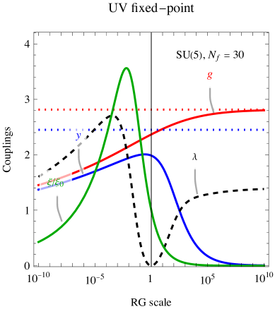
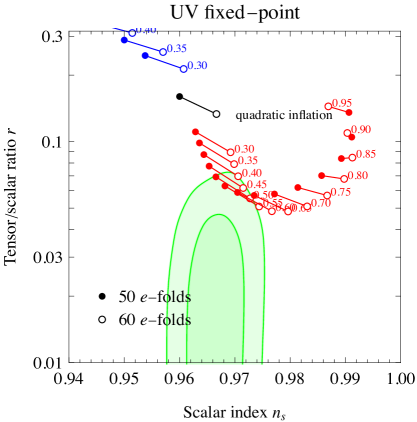
Figure 5: Left: Inflation with couplings that approach an interacting fixed point in the UV. Left: sample of RG running in the model of section 4.5 with $N=5$ and $N_{f}=29$. Right: its small-field (red) and large-field (blue) inflationary predictions for different values of $g_{0}/g_{*}$.

4.5 Inflation with an UV fixed-point

As we are interested in moderately large couplings that avoid Landau poles, the remaining possibility is asymptotic safety: dimension-less couplings that run up to an interacting UV fixed-point. Litim and Sannino [36] found that this is perturbatively realised in specific models, where the one-loop gauge beta function coefficient $b$ is small and negative, and the two-loop term is positive thanks to the contribution of a Yukawa coupling $y^{\prime}$ that reaches its UV fixed-point. As a result the gauge coupling runs according to eq. (46), where now $b<0$. The models involve a $\,{\rm SU}(N)$ gauge theory with $N_{f}$ Weyl fermions in $N\oplus\bar{N}$ and $N_{F}^{2}$ neutral scalars $S_{ij}$ with (for simplicity) a common Yukawa $y\,S_{ij}\psi_{i}\psi_{j}^{c}$. Since the scalars $S_{ij}$ are neutral, their scalar potential does not give rise to the desired post-inflationary SM minimum.

Following [37], we thereby add an extra inflation-candidate scalar $\Phi$ in the fundamental of $\,{\rm SU}(N)$, with a Yukawa coupling to one fermion flavour, as in eq. (47). We can assume, for simplicity, that the mixed scalar quartic $|\Phi|^{2}|S_{ij}|^{2}$ vanishes. Then the RG equations for $y,\lambda,\xi$ are as in eq.s (48).

Fig. 5a shows an example of the running tuned in such a way that the Einstein potential has the desired SM minimum at $\phi=\phi_{0}$ where $g=g_{0}$. We assumed $N=5$ colours, $N_{f}=30$ flavours (such that the UV fixed-point of $g_{*}$ is moderately large, allowing for significant deviations from the weak coupling limit), $\bar{y}=y$ and $g_{0}/g_{*}=0.5$. Fig. 5b shows the resulting inflationary predictions as function of $g_{0}/g_{*}$. Large-field inflation (in blue) gives too large $r$, small-field inflation (in red) allows acceptable values of $r$ but not below $r=0.05$ because when $g_{0}$ gets so large that details of the theory matter, the predicted $n_{s}$ and $r$ start deviating from the best-fit values. A similar result is found for different number of colours $N$.

5 Conclusions

A pole in the kinetic terms of one scalar $\phi$ leads to pole inflation. We explored the possibility that the same phenomenon arises in theories without poles in the Jordan frame, but rather in the Einstein frame originating from a non-minimal coupling of a scalar $f(\phi)$ to gravity. Points in field space where $f=0$ (namely, where gravity is strongly coupled) lead to pole inflation provided that the Jordan-frame scalar potential vanishes fast enough at the pole. In this case, pole inflation is recovered through the usual “stretching” of the canonicalised field. The needed condition on the potential is non-generic, and similar to the vanishing of the cosmological constant at the SM minimum.

We next explored the generic case with $N$ scalars $\phi^{i}$, where we found that the pole is generically promoted to a singularity curve, the ($N-1$)-dimensional surface where the non-minimal coupling vanishes, $f(\phi_{i})=0$. We describe the required form of the Jordan frame potential such that the multi-field generalisation of pole inflation is realised: the potential needs to vanish fast enough around at least one point of this surface. The field space is now generically warped, but the curvature is generically finite at and near the singularity surface and has negligible effects. The inflationary trajectory asymptotically approaches the singularity surface with an angle of incidence that depends on the potential. This modifies the effective residue at the pole. Up to this caveat, one obtains the usual attractor predictions that depend solely on the order and the residue of the pole. The pole has 2nd order and a universal residue whenever $f(\phi_{i})$ is approximatively linear around $f=0$. Assuming an approximately linear tilt in the potential, this gives the same predictions as Starobinsky inflation.

At first glance, the above situation has two unsatisfactory aspects:

1. The predictions of pole inflation arise assuming that inflation is fully dominated by field values around the pole, so that the structure of the potential around the SM minimum is neglected.

2. Canonicalisation of the graviton (namely, going from a generic Jordan frame to the Einstein frame) gives rise to pole inflation only if the potential has a non-generic structure.

In section 4 we showed that the needed structure of the potential automatically arises in quantum theories with dimension-less couplings only. A small tilt is provided by their RG running that lifts the exact flatness of the classical potential. Having a physical origin for the tilt, we can thereby abandon the assumption that inflation is fully dominated by the pole, and consider theories where the SM minimum is present and affects inflationary predictions. Small couplings universally lead to slow RG running and to nearly-quadratic inflation, that predicts a too large tensor/scalar ratio. We thereby consider larger couplings that provide the possible faster RG running that can arise in QFT: a coupling that runs either to a perturbative fixed point or to non-perturbative values, either in the UV (figures 2, 5) or in the IR (figures 3, 4). We then found that some of these models can provide acceptable inflationary predictions. In all the considered models, RG coefficients are such that the non-minimal coupling $\xi$ to gravity runs to smaller values at higher scales. Different models where $\xi$ runs in the opposite way could give different predictions.

Acknowledgements

This work was supported by the ERC grant 669668 NEO-NAT.

References

- [1] R. Kallosh, A. Linde and D. Roest, “Large field inflation and double -attractors”, JHEP 08 (2014) 052 [\IfBeginWith1405.364610.doi:1405.3646\IfSubStr1405.3646:InSpire:1405.3646arXiv:1405.3646].
- [2] R. Kallosh and A. Linde, “Planck, LHC, and -attractors”, Phys. Rev. D 91 (2015) 083528 [\IfBeginWith1502.0773310.doi:1502.07733\IfSubStr1502.07733:InSpire:1502.07733arXiv:1502.07733].
- [3] J. J. M. Carrasco, R. Kallosh and A. Linde, “Cosmological Attractors and Initial Conditions for Inflation”, Phys. Rev. D 92 (2015) no.6, 063519 [\IfBeginWith1506.0093610.doi:1506.00936\IfSubStr1506.00936:InSpire:1506.00936arXiv:1506.00936].
- [4] M. Rinaldi, L. Vanzo, S. Zerbini and G. Venturi, “Inflationary quasiscale-invariant attractors”, Phys. Rev. D 93 (2016) 024040 [\IfBeginWith1505.0338610.doi:1505.03386\IfSubStr1505.03386:InSpire:1505.03386arXiv:1505.03386].
- [5] A. Linde, “Single-field -attractors”, JCAP 05 (2015) 003 [\IfBeginWith1504.0066310.doi:1504.00663\IfSubStr1504.00663:InSpire:1504.00663arXiv:1504.00663].
- [6] K. Dimopoulos, C. Owen, “Quintessential Inflation with -attractors”, JCAP 06 (2017) 027 [\IfBeginWith1703.0030510.doi:1703.00305\IfSubStr1703.00305:InSpire:1703.00305arXiv:1703.00305].
- [7] B. J. Broy, M. Galante, D. Roest and A. Westphal, “Pole inflation – Shift symmetry and universal corrections”, JHEP 12 (2015) 149 [\IfBeginWith1507.0227710.doi:1507.02277\IfSubStr1507.02277:InSpire:1507.02277arXiv:1507.02277].
- [8] T. Terada, “Generalized Pole Inflation: Hilltop, Natural, and Chaotic Inflationary Attractors”, Phys.Lett.B 760 (2016) 674 [\IfBeginWith1602.0786710.doi:1602.07867\IfSubStr1602.07867:InSpire:1602.07867arXiv:1602.07867].
- [9] R. Kallosh and A. Linde, “Superconformal generalizations of the Starobinsky model”, JCAP 06 (2013) 028 [\IfBeginWith1306.321410.doi:1306.3214\IfSubStr1306.3214:InSpire:1306.3214arXiv:1306.3214].
- [10] J. J. M. Carrasco, R. Kallosh, A. Linde and D. Roest, “Hyperbolic geometry of cosmological attractors”, Phys. Rev. D 92 (2015) no.4, 041301 [\IfBeginWith1504.0555710.doi:1504.05557\IfSubStr1504.05557:InSpire:1504.05557arXiv:1504.05557].
- [11] S. D. Odintsov and V. K. Oikonomou, “Inflationary -attractors from gravity”, Phys. Rev. D 94 (2016) no.12, 124026 [\IfBeginWith1612.0112610.doi:1612.01126\IfSubStr1612.01126:InSpire:1612.01126arXiv:1612.01126].
- [12] S. D. Odintsov and V. K. Oikonomou, “Attractor cosmology from nonminimally coupled gravity”, Phys. Rev. D 97 (2018) no.6, 064005 [\IfBeginWith1802.0648610.doi:1802.06486\IfSubStr1802.06486:InSpire:1802.06486arXiv:1802.06486].
- [13] J. Kim and J. McDonald, “Chaotic initial conditions for nonminimally coupled inflation via a conformal factor with a zero”, Phys. Rev. D 95 (2017) no.10, 103501 [\IfBeginWith1612.0473010.doi:1612.04730\IfSubStr1612.04730:InSpire:1612.04730arXiv:1612.04730].
- [14] A. Salvio, A. Strumia, “Agravity”, JHEP 06 (2014) 080 [\IfBeginWith1403.422610.doi:1403.4226\IfSubStr1403.4226:InSpire:1403.4226arXiv:1403.4226].
- [15] K. Kannike, G. Hütsi, L. Pizza, A. Racioppi, M. Raidal, A. Salvio, A. Strumia, “Dynamically Induced Planck Scale and Inflation”, JHEP 05 (2015) 065 [\IfBeginWith1502.0133410.doi:1502.01334\IfSubStr1502.01334:InSpire:1502.01334arXiv:1502.01334].
- [16] D. Burns, S. Karamitsos and A. Pilaftsis, “Frame-Covariant Formulation of Inflation in Scalar-Curvature Theories”, Nucl. Phys. B 907 (2016) 785-819 [\IfBeginWith1603.0373010.doi:1603.03730\IfSubStr1603.03730:InSpire:1603.03730arXiv:1603.03730].
- [17] S. Karamitsos and A. Pilaftsis, “Frame Covariant Nonminimal Multifield Inflation”, Nucl. Phys. B 927 (2018) 219-254 [\IfBeginWith1706.0701110.doi:1706.07011\IfSubStr1706.07011:InSpire:1706.07011arXiv:1706.07011].
- [18] Planck collaboration, “Planck constraints on the tensor-to-scalar ratio”, Astron.Astrophys. 647 (2021) A128 [\IfBeginWith2010.0113910.doi:2010.01139\IfSubStr2010.01139:InSpire:2010.01139arXiv:2010.01139].
- [19] M. Galante, R. Kallosh, A. Linde, D. Roest, “Unity of Cosmological Inflation Attractors”, Phys.Rev.Lett. 114 (2015) 141302 [\IfBeginWith1412.379710.doi:1412.3797\IfSubStr1412.3797:InSpire:1412.3797arXiv:1412.3797].
- [20] R. Kallosh, A. Linde, “Universality Class in Conformal Inflation”, JCAP 07 (2013) 002 [\IfBeginWith1306.522010.doi:1306.5220\IfSubStr1306.5220:InSpire:1306.5220arXiv:1306.5220].
- [21] R. Kallosh, A. Linde, D. Roest, “Superconformal Inflationary -Attractors”, JHEP 11 (2013) 198 [\IfBeginWith1311.047210.doi:1311.0472\IfSubStr1311.0472:InSpire:1311.0472arXiv:1311.0472].
- [22] D.I. Kaiser, “Conformal Transformations with Multiple Scalar Fields”, Phys.Rev.D 81 (2010) 084044 [\IfBeginWith1003.115910.doi:1003.1159\IfSubStr1003.1159:InSpire:1003.1159arXiv:1003.1159].
- [23] S. Karamitsos, “Beyond the Poles in Attractor Models of Inflation”, JCAP 09 (2019) 022 [\IfBeginWith1311.047210.doi:1311.0472\IfSubStr1311.0472:InSpire:1311.0472arXiv:1311.0472].
- [24] D. Wands, N. Bartolo, S. Matarrese and A. Riotto, “An Observational test of two-field inflation”, Phys. Rev. D 66 (2002) 043520 [\IfBeginWithastro-ph/020525310.doi:astro-ph/0205253\IfSubStrastro-ph/0205253:InSpire:astro-ph/0205253arXiv:astro-ph/0205253].
- [25] G.N. Felder, L. Kofman, A.D. Linde, “Instant preheating”, Phys.Rev.D 59 (1999) 123523 [\IfBeginWithhep-ph/981228910.doi:hep-ph/9812289\IfSubStrhep-ph/9812289:InSpire:hep-ph/9812289arXiv:hep-ph/9812289].
- [26] L. H. Ford, “Gravitational particle creation and inflation”, Phys. Rev. D 35 (1987) 2955
- [27] K. Nakayama, K. Saikawa, T. Terada, M. Yamaguchi, “Structure of Kähler potential for D-term inflationary attractor models”, JHEP 05 (2016) 067 [\IfBeginWith1603.0255710.doi:1603.02557\IfSubStr1603.02557:InSpire:1603.02557arXiv:1603.02557].
- [28] T. Kobayashi, O. Seto, T. H. Tatsuishi, “Toward pole inflation and attractors in supergravity: Chiral matter field inflation”, Progress of Theoretical and Experimental Physics 2017 (2017) 12
- [29] S. Dimopoulos, S. Kachru, J. McGreevy and J. G. Wacker, “N-flation”, JCAP 08 (2008) 003
- [30] M. Dias, J. Frazer, A. Retolaza, M. Scalisi and A. Westphal, “Pole N-flation”, JHEP 02 (2019) 120
- [31] G. K. Karananas and J. Rubio, “On the geometrical interpretation of scale-invariant models of inflation”, Phys. Lett. B 761 (2016) 223-228 [\IfBeginWith1606.0884810.doi:1606.08848\IfSubStr1606.08848:InSpire:1606.08848arXiv:1606.08848].
- [32] A. Bedroya, C. Vafa, “Trans-Planckian Censorship and the Swampland”, JHEP 09 (2020) 123 [\IfBeginWith1909.1106310.doi:1909.11063\IfSubStr1909.11063:InSpire:1909.11063arXiv:1909.11063].
- [33] Z. Komargodski, A. Schwimmer, “On Renormalization Group Flows in Four Dimensions”, JHEP 12 (2011) 099 [\IfBeginWith1107.398710.doi:1107.3987\IfSubStr1107.3987:InSpire:1107.3987arXiv:1107.3987].
- [34] M.A. Luty, J. Polchinski, R. Rattazzi, “The -theorem and the Asymptotics of 4D Quantum Field Theory”, JHEP 01 (2013) 152 [\IfBeginWith1204.522110.doi:1204.5221\IfSubStr1204.5221:InSpire:1204.5221arXiv:1204.5221].
- [35] T. Banks, A. Zaks, “On the Phase Structure of Vector-Like Gauge Theories with Massless Fermions”, Nucl.Phys.B 196 (1982) 189
- [36] D.F. Litim, F. Sannino, “Asymptotic safety guaranteed”, JHEP 12 (2014) 178 [\IfBeginWith1406.233710.doi:1406.2337\IfSubStr1406.2337:InSpire:1406.2337arXiv:1406.2337].
- [37] G.M. Pelaggi, F. Sannino, A. Strumia, E. Vigiani, “Naturalness of asymptotically safe Higgs”, Front.in Phys. 5 (2017) 49 [\IfBeginWith1701.0145310.doi:1701.01453\IfSubStr1701.01453:InSpire:1701.01453arXiv:1701.01453].