Assured Neural Network Architectures for Control and Identification of Nonlinear Systems

Abstract

In this paper, we consider the problem of automatically designing a Rectified Linear Unit (ReLU) Neural Network (NN) architecture (number of layers and number of neurons per layer) with the assurance that it is sufficiently parametrized to control a nonlinear system; i.e. control the system to satisfy a given formal specification. This is unlike current techniques, which provide no assurances on the resultant architecture. Moreover, our approach requires only limited knowledge of the underlying nonlinear system and specification. We assume only that the specification can be satisfied by a Lipschitz-continuous controller with a known bound on its Lipschitz constant; the specific controller need not be known. From this assumption, we bound the number of affine functions needed to construct a Continuous Piecewise Affine (CPWA) function that can approximate any Lipschitz-continuous controller that satisfies the specification. Then we connect this CPWA to a NN architecture using the authors’ recent results on the Two-Level Lattice (TLL) NN architecture; the TLL architecture was shown to be parameterized by the number of affine functions present in the CPWA function it realizes.

1 Introduction

Recent advances in theory and computation have facilitated wide-spread adoption of Rectified Linear Unit (ReLU) Neural Networks (NNs) in conventional feedback-control settings, especially for Cyber-Physical Systems (CPSs) [1]. However, this proliferation of NN controllers has also highlighted weaknesses in state-of-the-art NN design techniques, because CPS systems are often safety critical. In a safety-critical CPS, it is not enough to simply learn a NN controller, i.e. fit data: such a controller must also have demonstrable safety or robustness properties, usually with respect to closed-loop specifications on a dynamical system. Moreover, a meaningful safety specification for a CPS is often binary: either a controller makes the system safe or it doesn’t. This is in contrast to optimization-based approaches typical in Machine/Reinforcement Learning (ML/RL), where the goal is to optimize a particular cost or reward without any requirements imposed on eventual quantity in question. Examples of the former include stability about an equilibrium point or forward invariance of a particular set of safe states (e.g. for collision avoidance). Examples of the latter include minimizing the mean-squared fit error; minimizing regret; or maximizing a surrogate for a value function; etc.

The distinction between safety specifications and ML/RL objectives is relevant to more than just learning NN weights and biases, though: it is has special relevance to NN architecture design — i.e. deciding on the number of neurons and their connection (or arrangement) in the NN to be trained in the first place. Specifically, (binary) safety specifications beg existential questions about NN architectures in a way that conventional, optimization-focused ML/RL techniques do not: given a particular NN architecture for a controller, it is necessary to ask whether there is there any possible choice of weights and biases that achieve the desired safety specification. By contrast, conventional ML/RL type problems instead take an architecture as given, and attempt to achieve the best training error, reward, etc. subject to that implicit constraint. Thus, in typical ML/RL treatments, NN architectures merely adjust the final cost/reward, rather than leading to ill-posedness, such as can occur with a safety specification.

In this paper, we directly address the issue of whether a ReLU NN architecture is well-posed as a state-feedback controller for a given nonlinear system and closed-loop (safety) specification. That is we present a systematic methodology for designing a NN controller architecture that is guaranteed (or assured) to be able to meet a given closed-loop specification. Our approach provides such a guarantee contingent on the following properties of the system and specification:

1. the nonlinear system’s vector field is Lipschitz continuous with known Lipschitz constants;

2. there exists a Lipschitz continuous controller that satisfies the closed-loop specification robustly, and the Lipschitz constant of that controller is known (although the controller itself need not be known); and

3. the conjectured Lipschitz continuous controller makes a compact subset of the state space positive invariant.

The need to assume the existence of a controller is primarily to ensure that the specification is well-posed in general – i.e., for any controller, whether it is a NN or not; we will elaborate on the robustness in (ii) subsequently. Importantly, subject to these conditions, our approach can design a NN controller architecture with the following assurance: there exists neuron weights/biases for that architecture such that it can exactly meet the same specification as the assured non-NN controller (albeit non-robustly). Moreover, our proposed methodology requires only the information described above, so it is applicable even without perfect knowledge of the underlying system dynamics, albeit at the expense of designing rather larger architectures.

The cornerstone of our approach is a special ReLU NN architecture introduced by the authors in the context of another control problem: viz. the Two-Level Lattice (TLL) ReLU NN architecture [2]. A TLL NN, like all ReLU NNs, instantiates a Continuous, Piecewise Affine (CPWA) function, and hence implements one of finitely many local linear functions at each point in its domain; thus, its domain, like that of any CPWA, can be partitioned into linear regions, each of which corresponds to a different local linear function. However, unlike general ReLU NN architectures, a TLL NN exposes these local linear functions directly in the parameters of the network. As a consequence of this parameterization, then, TLL NNs are easily parameterized by their number of linear regions: after all, each linear region must instantiate at least one local linear function – see [2, Theorem 2]. In fact, this idea also applies to upper bounds on the number of regions desired in an architecture; see [2, Theorem 3]. TLL NNs thus have the special property that they can be used to connect a desired number of linear regions directly to a ReLU architecture.

Thus, to obtain an assured controller architecture, it is enough to obtain an assured upper-bound on the number of linear regions required of a controller. In this paper, we show that such an assured upper bound can be obtained using just the information assumed in (i) - (iii); i.e. primarily Lipschitz constants and bounds on the relevant objects. This bound is derived by counting the number of linear regions needed to linearly and continuously interpolate between regularly spaced “samples” of a controller with known Lipschitz constant.

Moreover, this core approach is relevant to end-to-end learning beyond just the design of controller architectures: it can also be used to obtain architectures that are guaranteed to represent the dynamics of a nonlinear system itself – i.e. assured architectures for system identification. Indeed, in this paper, we further show that contingent on information akin to (i) and (iii), it is possible to generate a ReLU architecture that is guaranteed to capture the essence of an unknown nonlinear control system. Specifically, we exhibit a methodology for designing an architecture to represent a nonlinear (controlled) vector field with the following assurance: if the ReLU vector field is sufficiently well trained on data from a compatible – but unknown – controlled vector field, then robustly controlling the ReLU dynamics to a specification will yield a controller that likewise controls the unknown dynamics to the same specification (albeit non-robustly). Providing a guaranteed architecture for system identification has unique value for end-to-end learning: because the ReLU control system can be used as a surrogate for the original nonlinear system, control design can be moved entirely from the unknown system to the known ReLU surrogate, the latter of which can be simulated instead. Furthermore, this system identification can be combined with a guaranteed controller architecture to do in silico ReLU control design.

The contributions of this paper can be summarized thusly.

1. A new notion of Abstract Disturbance Simulation (ADS) to formulate of robust specification satisfaction; ADS unifies and generalizes several related notions of simulation in the literature – see Section 3.2.

2. A methodology to design a ReLU architecture that is assured to be able to control an unknown nonlinear system to meet a closed-loop specification; this is subject to the existence of a (likewise) unknown controller that robustly meets the same specification.

3. A methodology to design a ReLU architecture that can be used in system identification of an unknown nonlinear control system; this architecture, when adequately trained, is assured to be viable as a surrogate for the original nonlinear system in controller design.

A preliminary version of this paper appeared as [3]. Relative to [3], this paper has the following additional novel content: first, it uses new, dramatically improved techniques to obtain a smaller architecture than [3] (see Remark 3); second, it includes full proofs of every claim; and third, it contains the extension to system identification architectures noted above.

1.1 Related Work

The literature most directly relevant to this paper is work by the authors: AReN [2] and the preliminary version of this paper, [3]. The former contains an algorithm that generates an architecture assured to represent an optimal MPC controller. The AReN algorithm is fully automatic, and the assurances provided are the same as those for the referent MPC controller; but it is not very generalizable, given the restriction to MPC control. This paper and its preliminary version offer a significantly improved methodology. The architecture design presented herein is likewise fully automatic; however, it is generalizable to any Lipschitz continuous control system, and it provides assurances for a wide variety specification captured by simulation relations.

The largest single class of NN architecture design algorithms is commonly referred to as Neural Architecture Search (NAS) algorithms. These algorithms essentially use an iterative improvement/optimization scheme to design a NN architecture, thus automating something like a ‘guess-train-evaluate” hyperparameter tuning loop. There is a large literature on NAS algorithms; [4] is a good summary. Typical NASs design architectures within some structured class of architectures such as: “chain” architectures (i.e. a sequence of fully connected layers) [5]; chain architectures with different layer types (e.g. convolution, pooling, etc. in addition to fully connected) [6, 7]; or mini-NN architectures that are replicated and interconnected to form larger networks [8]. They then update these architectures according to a variety of different mechanisms: RL formulations [9, 10, 8]; sequential decision problems formulations where actions corresponding to network morphisms [7]; Bayesian optimization formulations [11, 5]; and Neuro-evolutionary approaches (relatedly population dynamics or genetic algorithms) [12, 13]. Different evaluation mechanisms are used to evaluate the “quality” of current architecture iterate: lower fidelity models [8] or weight inheritance morphisms [4, 7] (a sort of transfer learning); learning curve extrapolation to estimate the final performance of an architecture before training has converged [6]; and one-shot models that agglomerate many architectures into a single large architecture that shares edges between individual architectures [14]. Notably these algorithms all share the same features: they are highly automatic, even accounting for the need to choose meta-hyperparameters; they are fairly general, since they are data-driven; however, they provide no closed-loop assurances.

At the opposite end of our assessment spectra are control-based methods for obtaining NN controllers with assurances; we regard these methods as implicit architecture design techniques, since exhibiting a NN controller serves as a direct validation of that controller’s architecture. Examples of these methods include: directly approximating a controller by a NN for non-affine systems [15]; adaptively learning NN controller weights to ensure Input-to-State stability for certain third-order affine systems [16, 17]; NN hybrid adaptive control for stabilizing uncertain impulsive dynamical systems [18]. These methods are based on the assertion that a function of interest can be approximated by a sufficiently large (usually shallow) NN: the size of this NN is explicit, which limits their effectiveness as architecture design methods. Even neglecting this shortcoming, these methods generally provide just one meaningful assurance (stability); they are not at all general, since they are based on approximating a specific, hand-designed controller; and they are thus highly manual methods.

A subset of NN verification methods from the control system literature is related to the “guess-train-evaluate” architecture design iterations described above. In particular, some closed-loop NN verifiers provide additional dynamical information about how a NN controller fails to meet a specification. Examples include: using complementary analysis on NN-controlled linear systems, thus obtaining sufficient conditions for stability in terms of LMIs [19]; training and verifying a specific NN architecture as a barrier certificate for hybrid systems [20]; and using adversarial perturbation to verify NN control policies [21]. These methods can be assessed as follows: they are highly automatic (verifiers); they are of limited generalizability, since they require either specific models and/or detailed knowledge of the dynamical model; and each provides one and only one assurance (e.g. stability or a barrier certificate). A similar, but less applicable, subset of the control literature that consists of experimental work that suggests promising NN controller architectures. These works do not do automatic NN architecture design, nor do they contain verification algorithms of the type suggested above. Even so, they experimentally support using some conventional NN architectures as controllers [22]; and using Input Convex NNs (ICNNs) for controllers and system identification [23].

We also acknowledge prior work on system identification using NNs, although they do not emphasize architecture design. These methods suffer from a lack of assurances on the resultant NNs/architectures [24, 25, 26, 27].

Finally, subsequent to the publication of [3], we became aware of other works that use more or less what we describe as TLL NNs [28, 29]. The former is concerned with simplification of explicit MPC controllers rather than NN architecture design; the latter can be regarded as architecture design for a different application (although the architectures are less efficient than the ones presented here – see Remark 4).

2 Preliminaries

2.1 Notation

We denote by $\mathbb{N}$, $\mathbb{R}$ and $\mathbb{R}^{+}$ the set of natural numbers, the set of real numbers and the set of non-negative real numbers, respectively. For a function $f:A\rightarrow B$, let $\text{dom}(f)$ return the domain of $f$, and let $\text{range}(f)$ return the range of $f$. For $x\in\mathbb{R}^{n}$, we will denote by $\lVert x\rVert$ the max-norm of $x$. Relatedly, for $x\in\mathbb{R}^{n}$ and $\epsilon\geq 0$ we will denote by $B(x;\epsilon)$ the open ball of radius $\epsilon$ centered at $x$ as specified by $\lVert\cdot\rVert$, and $\overline{B}(x;\epsilon)$ its closed-ball analog. Let $\text{int}(X)$ denote the interior of a set $X\subseteq\mathbb{R}^{n}$, and $\text{bd}(X)=X\backslash\text{int}(X)$ denote its boundary. $e_{i}$ will denote the $i^{\text{th}}$ column of the $(n\times n)$ identity matrix, unless otherwise specified. Let $\text{hull}(X)$ denote the convex hull of a set of points $X\subseteq\mathbb{R}^{n}$. For $f:\mathbb{R}^{n}\rightarrow\mathbb{R}^{m}$, $\lVert f\rVert_{\infty}\triangleq\text{ess}\sup_{x\in\mathbb{R}^{n}}\lVert f(x)\rVert$, and $\lVert f\rVert_{X}$ will denote the same but restricted to the set $X$. The projection map over $\mathbb{R}^{n}$ will be denoted by $\pi_{i}:\mathbb{R}^{n}\rightarrow\mathbb{R}$, so that $\pi_{i}(x)$ returns the $i^{\text{th}}$ component of the vector $x$ (in the understood coordinate system). Finally, given two sets $A$ and $B$ denote by $B^{A}$ the set of all functions $f:A\rightarrow B$.

2.2 Dynamical Model

In this paper, we will assume an underlying, but not necessarily known, continuous-time nonlinear dynamical system specified by an ordinary differential equation (ODE): that is

$$\dot{x}(t)=f(x(t),u(t))$$ (1)

where the state vector $x(t)\in\mathbb{R}^{n}$ and the control vector $u(t)\in\mathbb{R}^{m}$. Formally, we have the following definition:

Definition 1 (Control System).

A control system is a tuple $\Sigma=(X,U,\mathcal{U},f)$ where

• $X\subset\mathbb{R}^{n}$ is the connected, compact subset of the state space with non-empty interior;

• $U\subset\mathbb{R}^{m}$ is the compact set of admissible controls;

• $\mathcal{U}\subseteq U^{\mathbb{R}^{+}}$ is the space of admissible open-loop control functions – i.e. $v\in\mathcal{U}$ is a function $v:\mathbb{R}^{+}\rightarrow U$; and

• $f:\mathbb{R}^{n}\times U\rightarrow\mathbb{R}^{n}$ is a vector field specifying the time evolution of states according to (1).

A control system is said to be (globally) Lipschitz if there exists constants $K_{x}$ and $K_{u}$ s.t. for all $x,x^{\prime}\in\mathbb{R}^{n}$ and $u,u^{\prime}\in\mathbb{R}^{m}$:

$$\lVert f(x,u)-f(x^{\prime},u^{\prime})\rVert\leq K_{x}\lVert x-x^{\prime}\rVert+K_{u}\lVert u-u^{\prime}\rVert.$$ (2)

In the sequel, we will primarily be concerned with solutions to (1) that result from instantaneous state-feedback controllers, $\Psi:X\rightarrow U$. Thus, we use $\zeta_{x_{0}\Psi}$ to denote the closed-loop solution of (1) starting from initial condition $x_{0}$ (at time $t=0$) and using state-feedback controller $\Psi$. We refer to such a $\zeta_{x_{0}\Psi}$ as a (closed-loop) trajectory of its associated control system.

Definition 2 (Closed-loop Trajectory).

Let $\Sigma$ be a Lipschitz control system, and let $\Psi:\mathbb{R}^{n}\rightarrow U$ be a globally Lipschitz continuous function. A closed-loop trajectory of $\Sigma$ under controller $\Psi$ and starting from $x_{0}\in X$ is the function $\zeta_{x_{0}\Psi}:\mathbb{R}^{+}\rightarrow X$ that solves the integral equation:

$$\zeta_{x_{0}\Psi}(t)=x_{0}+\int_{0}^{t}f(\zeta_{x_{0}\Psi}(\sigma),\Psi(\zeta_{x_{0}\Psi}(\sigma)))d\sigma.$$ (3)

It is well known that such solutions exist and are unique under these assumptions [30].

Definition 3 (Feedback Controllable).

A Lipschitz control system $\Sigma$ is feedback controllable by a Lipschitz controller $\Psi:\mathbb{R}^{n}\rightarrow U$ if the following is satisfied:

$$\Psi\circ\zeta_{x\Psi}\in\mathcal{U}\qquad\forall x\in X.$$ (4)

If $\Sigma$ is feedback controllable for any such $\Psi$, then we simply say that it is feedback controllable.

Because we’re interested in a compact set of states, $X$, we consider only feedback controllers whose closed-loop trajectories stay within $X$.

Definition 4 (Positive Invariance).

A feedback trajectory of a Lipschitz control system, $\zeta_{x_{0}\Psi}$, is positively invariant if $\zeta_{x_{0}\Psi}(t)\in X$ for all $t\geq 0$. A controller $\Psi$ is positively invariant if $\zeta_{x_{0}\Psi}$ is positively invariant for all $x_{0}\in X$.

For technical reasons, we will also need the following stronger notion of positive invariance.

Definition 5 ($\delta$,$\tau$ Positive Invariance).

Let $\delta,\tau\negthinspace>\negthinspace 0$ and $\text{edge}_{\delta}(X)\negthinspace\triangleq\negthinspace\cup_{x\in X\backslash\text{int}(X)}(X\negthinspace\cap\negthinspace B(x;\delta))$. Then a positively invariant controller $\negthinspace\Psi\negthinspace$ is $\mathbf{\delta}$,$\mathbf{\tau}$ positively invariant if

$$\forall x_{0}\in\text{edge}_{\delta}(X)\;.\;\zeta_{x_{0}\negthinspace\Psi}(\tau)\negthinspace\in\negthinspace X\backslash\text{edge}_{\delta}(X)$$ (5)

and $\Psi$ is positively invariant with respect to $X\backslash\text{edge}_{\delta}(X)$.

For a $\delta$,$\tau$ positively invariant controller, trajectories that start $\delta$-close to the boundary of $X$ will end up $\delta$-far away from that boundary after $\tau$ seconds, and remain there forever after.

Finally, borrowing from [31], we define a $\tau$-sampled transition system embedding of a feedback-controlled system.

Definition 6 ($\tau$-sampled Transition System Embedding).

Let $\Sigma=(X,U,\mathcal{U},f)$ be a feedback controllable Lipschitz control system, and let $\Psi:\mathbb{R}^{n}\rightarrow U$ be a Lipschitz continuous feedback controller. For any $\tau>0$, the $\mathbf{\tau}$-sampled transition system embedding of $\Sigma$ under $\Psi$ is the tuple $S_{\tau}(\Sigma_{\Psi})=(X_{\tau},\mathcal{U}_{\tau},\overset{~{}}{{}_{\scriptscriptstyle\Sigma_{\Psi}}\negthickspace\negthickspace\negthinspace\negthinspace\longrightarrow})$ where:

• $X_{\tau}=X$ is the state space;

• $\mathcal{U}_{\tau}=\{(\Psi\circ\zeta_{x_{0}\Psi})|_{t\in[0,\tau]}:x_{0}\in X\}$ is the set of open loop control inputs generated by $\Psi$-feedback, each restricted to the domain $[0,\tau]$; and

• $\overset{~{}}{{}_{\scriptscriptstyle\Sigma_{\Psi}}\negthickspace\negthickspace\negthinspace\negthinspace\longrightarrow}\subseteq X_{\tau}\times\mathcal{U}_{\tau}\times X_{\tau}$ such that $x\overset{u}{{}_{\scriptscriptstyle\Sigma_{\Psi}}\negthickspace\negthickspace\negthinspace\negthinspace\longrightarrow}x^{\prime}$ iff
         both $u=(\Psi\circ\zeta_{x\Psi})|_{t\in[0,\tau]}$ and $x^{\prime}=\zeta_{x\Psi}(\tau)$.

$S_{\tau}(\Sigma_{\Psi})$ is thus a metric transition system [31].

Definition 7 (Simulation Relation).

Let $S_{1}=(X_{1},\mathcal{U}_{1},\overset{~{}}{{}_{\scriptscriptstyle 1\vphantom{\scriptstyle(}}\negthickspace\negthickspace\negthinspace\longrightarrow})$ and $S_{2}=(X_{2},\mathcal{U}_{2},\overset{~{}}{{}_{\scriptscriptstyle 2\vphantom{\scriptstyle(}}\negthickspace\negthickspace\negthinspace\longrightarrow})$ be two metric transition systems. Then we say that $S_{2}$ simulates $S_{1}$, written $S_{1}\precsim S_{2}$, if there exists a relation $\precsim\subseteq X_{1}\times X_{2}$ such that

• $\{x_{1}|(x_{1},x_{2})\in\precsim\}=X_{1}$; and

• for all $(x_{1},x_{2})\in\precsim$ we have

  $$x_{1}\overset{u}{{}_{\scriptscriptstyle 1\vphantom{\scriptstyle(}}\negthickspace\negthickspace\negthinspace\longrightarrow}x_{1}^{\prime}\implies$$

  $$\qquad\qquad\exists x_{2}^{\prime}\in X_{2}.\big{(}(x_{1}^{\prime},x_{2}^{\prime})\in\precsim\;\wedge\;x_{2}\overset{u}{{}_{\scriptscriptstyle 2\vphantom{\scriptstyle(}}\negthickspace\negthickspace\negthinspace\longrightarrow}x_{2}^{\prime}\big{)}.$$ (6)

2.3 ReLU Neural Network Architectures

We will consider controlling the nonlinear system defined in (1) with a state-feedback neural network controller ${\mathscr{N}\negthickspace\negthickspace\negthinspace\mathscr{N}}\negthinspace$:

$${\mathscr{N}\negthickspace\negthickspace\negthinspace\mathscr{N}}\negthinspace:X\rightarrow U$$ (7)

where ${\mathscr{N}\negthickspace\negthickspace\negthinspace\mathscr{N}}\negthinspace$ denotes a Rectified Linear Unit Neural Network (ReLU NN). Such a ($K$-layer) ReLU NN is specified by composing $K$ layer functions (or just layers). A layer with $\mathfrak{i}$ inputs and $\mathfrak{o}$ outputs is specified by a $(\mathfrak{o}\times\mathfrak{i})$ matrix of weights, $W$, and a $(\mathfrak{o}\times 1)$ matrix of biases, $b$, as follows:

$$L_{\theta}:\mathbb{R}^{\mathfrak{i}} \rightarrow\mathbb{R}^{\mathfrak{o}}$$

$$z \mapsto\max\{Wz+b,0\}$$ (8)

where the $\max$ function is taken element-wise, and $\theta\triangleq(W,b)$ for brevity. Thus, a $K$-layer ReLU NN function is specified by $K$ layer functions $\{L_{\theta^{(i)}}:i=1,\dots,K\}$ whose input and output dimensions are composable: that is, they satisfy $\mathfrak{i}_{i}=\mathfrak{o}_{i-1}$ for $i=2,\dots,K$. Specifically:

$${\mathscr{N}\negthickspace\negthickspace\negthinspace\mathscr{N}}\negthinspace(x)=(L_{\theta^{(K)}}\circ L_{\theta^{(K-1)}}\circ\dots\circ L_{\theta^{(1)}})(x).$$ (9)

When we wish to make the dependence on parameters explicit, we will index a ReLU function ${\mathscr{N}\negthickspace\negthickspace\negthinspace\mathscr{N}}\negthinspace$ by a list of matrices $\Theta\triangleq(\theta^{(1)},\dots,\theta^{(K)})$ .

Fixing the number of layers and the dimensions of the associated matrices $\theta^{(i)}=(\;W^{(i)},b^{(i)}\;)$ specifies the architecture of a fully-connected ReLU NN. Therefore, we will use:

$$\text{Arch}(\Theta)\negthinspace\triangleq\negthinspace((n,\mathfrak{o}_{1}),(\mathfrak{i}_{2},\mathfrak{o}_{2}),\ldots,(\mathfrak{i}_{K},m))$$ (10)

to denote the architecture of the ReLU NN ${\mathscr{N}\negthickspace\negthickspace\negthinspace\mathscr{N}}\negthinspace_{\Theta}$.

Since we are interested in designing ReLU architectures, we will also need the following result from [2, Theorem 7], which states that a Continuous, Piecewise Affine (CPWA) function, $\mathsf{f}$, can be implemented exactly using a Two-Level-Lattice (TLL) NN architecture that is parameterized by the local linear functions in $\mathfrak{f}$.

Definition 8 (Local Linear Function).

Let $\mathsf{f}:\mathbb{R}^{n}\rightarrow\mathbb{R}^{m}$ be CPWA. Then a local linear function of $\mathsf{f}$ is a linear function $\ell:\mathbb{R}^{n}\rightarrow\mathbb{R}^{m}$ if there exists an open set $\mathfrak{O}\subseteq\mathbb{R}^{n}$ such that $\ell(x)=\mathsf{f}(x)$ for all $x\in\mathfrak{O}$.

Definition 9 (Linear Region).

Let $\mathsf{f}:\mathbb{R}^{n}\rightarrow\mathbb{R}^{m}$ be CPWA. Then a linear region of $\mathsf{f}$ is the largest set $\mathfrak{R}\subseteq\mathbb{R}^{n}$ such that $\mathsf{f}$ has only one local linear function on $\text{int}(\mathfrak{R})$.

Theorem 1 (Two-Level-Lattice (TLL) NN Architecture [7, Theorem 7]).

Let $\mathsf{f}:\mathbb{R}^{n}\rightarrow\mathbb{R}^{m}$ be a CPWA function, and let $\bar{N}$ be an upper bound on the number of local linear functions in $\mathsf{f}$. Then there is a Two-Level-Lattice (TLL) NN architecture $\text{Arch}(\Theta^{\overset{\text{\tiny TLL}}{~{}}}_{\bar{N}})$ parameterized by $\bar{N}$ and values of $\Theta^{\overset{\text{\tiny TLL}}{~{}}}_{\bar{N}}$ such that:

$$\mathsf{f}={\mathscr{N}\negthickspace\negthickspace\negthinspace\mathscr{N}}\negthinspace_{\negthickspace\Theta^{\overset{\text{\tiny TLL}}{~{}}}_{\bar{N}}}.$$ (11)

In particular, the number of linear regions of $\mathsf{f}$ is such an upper bound on the number of local linear functions.

In this paper, we will find it convenient to use Theorem 1 to create TLL architectures component-wise. To this end, we define the following notion of NN composition.

Definition 10.

Let ${\mathscr{N}\negthickspace\negthickspace\negthinspace\mathscr{N}}\negthinspace_{\Theta_{\scriptscriptstyle 1}}$ and ${\mathscr{N}\negthickspace\negthickspace\negthinspace\mathscr{N}}\negthinspace_{\Theta_{\scriptscriptstyle 2}}$ be two $K$-layer NNs with parameter lists:

$$\Theta_{i}=((W^{\scriptscriptstyle|1}_{i},b^{\scriptscriptstyle|1}_{i}),\dots,(W^{\scriptscriptstyle|K}_{i},b^{\scriptscriptstyle|K}_{i})),\quad i=1,2.$$ (12)

Then the parallel composition of ${\mathscr{N}\negthickspace\negthickspace\negthinspace\mathscr{N}}\negthinspace_{\Theta_{\scriptscriptstyle 1}}$ and ${\mathscr{N}\negthickspace\negthickspace\negthinspace\mathscr{N}}\negthinspace_{\Theta_{\scriptscriptstyle 2}}$ is a NN given by the parameter list

$$\Theta_{1}\parallel\Theta_{2}\triangleq\big{(}\negthinspace\left(\negthinspace\left[\begin{smallmatrix}W^{\scriptscriptstyle|1}_{1}\\ W^{\scriptscriptstyle|1}_{2}\end{smallmatrix}\right],\left[\begin{smallmatrix}b^{\scriptscriptstyle|1}_{1}\\ b^{\scriptscriptstyle|1}_{2}\end{smallmatrix}\right]\negthinspace\right),{\scriptstyle\dots},\left(\negthinspace\left[\begin{smallmatrix}W^{\scriptscriptstyle|K}_{1}\\ W^{\scriptscriptstyle|K}_{2}\end{smallmatrix}\right],\left[\begin{smallmatrix}b^{\scriptscriptstyle|K}_{1}\\ b^{\scriptscriptstyle|K}_{2}\end{smallmatrix}\right]\negthinspace\right)\negthinspace\big{)}.$$ (13)

That is $\Theta_{1}\negthickspace\parallel\negthickspace\Theta_{2}$ accepts an input of the same size as (both) $\Theta_{1}$ and $\Theta_{2}$, but has as many outputs as $\Theta_{1}$ and $\Theta_{2}$ combined.

Corollary 1.

Let $\mathsf{f}:\mathbb{R}^{n}\rightarrow\mathbb{R}^{m}$ be a CPWA function, each of whose $m$ component CPWA functions are denoted by $\mathsf{f}_{i}:x\mapsto\pi_{i}(\mathsf{f}(x))$, and let $\bar{N}$ be an upper bound on the number of linear regions in each $\mathsf{f}_{i}$.

Then for $\Theta^{\overset{\text{\tiny TLL}}{~{}}}_{\bar{N}}$ a TLL architecture representing a CPWA $\mathbb{R}^{n}\rightarrow\mathbb{R}$, the $m$-fold parallel TLL architecture:

$$\Theta^{\overset{\text{\tiny TLL}\parallel}{~{}}}_{{}^{n}_{m}\negthinspace\bar{N}}\triangleq\Theta^{\overset{\text{\tiny TLL}}{~{}}}_{\bar{N}}\parallel\dots\parallel\Theta^{\overset{\text{\tiny TLL}}{~{}}}_{\bar{N}}$$ (14)

has the property that $\mathsf{f}={\mathscr{N}\negthickspace\negthickspace\negthinspace\mathscr{N}}\negthinspace_{\Theta^{\overset{\text{\tiny TLL}\parallel}{~{}}}_{{}^{n}_{m}\negthinspace\bar{N}}}$.

Proof.

Apply Theorem 1 component-wise. ∎

Finally, note that a ReLU NN function, ${\mathscr{N}\negthickspace\negthickspace\negthinspace\mathscr{N}}\negthinspace$, is known to be a continuous, piecewise affine (CPWA) function consisting of finitely many linear segments. Thus, a function ${\mathscr{N}\negthickspace\negthickspace\negthinspace\mathscr{N}}\negthinspace$ is itself necessarily globally Lipschitz continuous.

2.4 Notation Pertaining to Hypercubes

Since the unit ball of the max-norm, $\lVert\cdot\rVert$, on $\mathbb{R}^{n}$ is a hypercube, we will make use of the following notation.

Definition 11 (Face/Corner of a hypercube).

Let $C_{n}=[0,1]^{n}$ be a unit hypercube of dimension $n$. A set $F\subseteq C_{n}$ is a $k$-dimensional face of $C_{n}$ if there exists a set $J\subseteq\{1,\negthinspace\dots,\negthinspace n\}$ such that $|J|=n\negthinspace-\negthinspace k$ and

$$\forall x\in F~{}.~{}\bigwedge_{j\in J}\Big{(}\pi_{j}(x)\in\{0,1\}\Big{)}.$$ (15)

Let $\mathscr{F}_{k}(C_{n})$ denote the set of $k$-dimensional faces of $C_{n}$, and let $\mathscr{F}(C_{n})$ denote the set of all faces of $C_{n}$ (of any dimension). A corner of $C_{n}$ is a $0$-dimensional face of $C_{n}$. Furthermore, we will use the notation $F_{i}^{k}$ to denote an full-dimensional face ($n-1$-dimensional in this case) whose index set $J=\{i\}$ and whose projection on the $i^{\text{th}}$ coordinate is $k\in\{0,1\}$.

We extend these definitions by isomorphism to any other hypercube in $\mathbb{R}^{n}$.

3 Problem Formulation: NN Architectures for Control

We begin by stating the first main problem that we will consider in this paper: that of designing an assured NN architecture for nonlinear control (hereafter referred to as the controller architecture problem). Specifically, we wish to identify a ReLU architecture to be used as a feedback controller for the control system $\Sigma$; this architecture must further come with the assurance that there exist parameter weights for which the realized NN controller controls $\Sigma$ to some proscribed specification.

However, for pedagogical reasons, we will state two versions of the controller architecture problem in this section. The first will be somewhat generic in order to motivate a crucial innovation of this paper: a new simulation relation, Abstract Disturbance Simulation (ADS) (see also [3]). The second formulation of this problem, then, actually incorporates ADS into a formal problem statement, where it serves to facilitate the design of assured controller architectures. Our solution of this second, more specific version, is the main contribution of this paper, and appears as Theorem 2 in Section 4.

3.1 Generic Controller Architecture Problem

As noted in Section 1, designing an assured NN architecture for control hinges on the well-posedness of the desired (binary) closed-loop specification, and this is as much a statement about the specification as it is about the architecture. Thus, a formal problem of NN architecture design (for control) necessarily begins with a framework for describing closed-loop system specifications.

To this end, we will formulate our controller architecture problem in terms of a $\tau$-sampled metric transition system embedding of the underlying continuous-time models (see Section 2.2). Although this choice may seem an unnatural deviation from the underlying continuous-time models, it affords two important benefits. First, metric transition systems come with a natural and flexible notion of specification satisfaction in the form of (bi)simulation relations. In this paradigm, specifications are described by means of another transition system that encodes the specification; the original system then satisfies the specification if it is simulated by the (transition system) encoding of the specification. Importantly, it is well known that a diverse array of specifications can be captured in this context, among them LTL formula satisfaction [32] and stability. Secondly, the sample period $\tau$ constitutes an additional degree of freedom in the specification relative to the original continuous-time system (or a proscribed fixed sample-period embedding); this extra degree of freedom will facilitate the development of assured NN architectures.

From this, we consider the following generic formulation of a controller architecture design problem.

Problem 1 (Controller Architecture Design – Generic Formulation).

Let $\tau>0$ and $K_{\text{cont}}\negthinspace>\negthinspace 0$ be given. Let $\Sigma$ be a feedback controllable Lipschitz control system, and let $S_{\text{spec}}\negthinspace=\negthinspace(X_{\text{spec}},U_{\text{spec}},\overset{~{}}{{}_{\scriptscriptstyle S_{\text{spec}}\negthickspace\negthickspace\vphantom{\scriptstyle(}}\negthickspace\negthickspace\negthinspace\longrightarrow})$ be a transition system encoding for a specification on $\Sigma$.

Now, suppose that there exists a Lipschitz-continuous controller $\Psi:\mathbb{R}^{n}\rightarrow U$ with Lipschitz constant $K_{\Psi}\leq K_{\text{cont}}$ s.t.:

$$S_{\tau}(\Sigma_{\Psi})\preceq S_{\text{spec}}.$$ (16)

Then the problem is to find a ReLU architecture, $\text{Arch}(\Theta)$, with the property that there exists values for $\Theta$ such that:

$$S_{\tau}(\Sigma_{\negthinspace{\mathscr{N}\negthickspace\negthickspace\negthinspace\mathscr{N}}\negthinspace\negthinspace_{\Theta}})\preceq S_{\text{spec}}.$$ (17)

In both (16) and (17), $\precsim$ is as defined in Definition 7.

The main assumption in 1 is that there exists a controller $\Psi$ which satisfies the specification, $S_{\text{spec}}$. We use this assumption primarily to help ensure that the problem is well posed: indeed, it is known that there are nonlinear control problems for which no continuous controllers exits. Thus, this assumption is in some sense an essential requirement to formulate a well-posed controller architecture problem: for if there exists no such $\Psi$, then there could be no NN controller that satisfies the specification, either, since the latter also belongs to the class of Lipschitz continuous functions (modulo discrepancies in Lipschitz constants). In this way, the existence of a controller $\Psi$ also subsumes any possible conditions on the nonlinear system that one might wish to impose: stabilizability, for example.

That 1 is more or less ill-posed without assuming the existence of a controller $\Psi$ (for some constant $K_{\text{cont}}$) suggests a natural solution to the problem. In particular, a NN architecture can be bootstrapped from this knowledge by simply designing an architecture that is sufficiently parameterized as to adequately approximate any such $\Psi$, i.e. any function of Lipschitz constant at most $K_{\text{cont}}$ (this is a preview of the approach we will subsequently use). Unfortunately, however, this approach also reveals a deficiency in the assumption associated with $\Psi$: controller approximation necessarily introduces instantaneous control errors relative to $\Psi$, and these errors can compound transition upon transition from the dynamics. As a consequence, the assumed information about $\Psi$ is actually not as immediately helpful as it appears. In particular, if $\Psi$ is not very robust, then the accumulation of such errors could make it impossible to prove that an (approximate) NN controller satisfies the same specification as $\Psi$, viz. (17).

This effect can be seen directly in terms of the simulation relations in (16) and (17). Take $x\in X_{\tau}$ and consider two transitions from $x$: one in $S_{\tau}(\Sigma_{\Psi})$ given by $x\overset{~{}}{{}_{\scriptscriptstyle\Sigma_{\Psi}}\negthickspace\negthickspace\negthinspace\negthinspace\longrightarrow}x^{\prime}$ and one in $S_{\tau}(\Sigma_{\negthinspace{\mathscr{N}\negthickspace\negthickspace\negthinspace\mathscr{N}}\negthinspace\negthinspace_{\Theta}})$ given by $x\overset{~{}}{{}_{\scriptscriptstyle\Sigma_{\negthinspace{{\mathscr{N}\negthickspace\negthickspace\negthinspace\mathscr{N}}\negthinspace_{\Theta}}}}\negthickspace\negthickspace\negthinspace\negthinspace\longrightarrow}x^{\prime\prime}$. Note that if ${\mathscr{N}\negthickspace\negthickspace\negthinspace\mathscr{N}}\negthinspace_{\Theta}$ merely approximates $\Psi$, there will in general be a discrepancy between $x^{\prime}$ and $x^{\prime\prime}$, i.e. $x^{\prime}\neq x^{\prime\prime}$. Thus, although $x^{\prime}$ necessarily has a simulating state in $S_{\text{spec}}$ by assumption, $x^{\prime\prime}$ need not have its own simulating state in $S_{\text{spec}}$. This follows because the simulation relation in Definition 7 can assert simulating states only through transitions (i.e. (6)), and there may be no transition $x\overset{~{}}{{}_{\scriptscriptstyle\Sigma_{\Psi}}\negthickspace\negthickspace\negthinspace\negthinspace\longrightarrow}x^{\prime\prime}$ in $S_{\tau}(\Sigma_{\Psi})$.

3.2 Abstract Disturbance Simulation

Motivated by the observations above, we propose a new simulation relation as a formal notion of specification satisfaction for metric transition systems; we call this relation abstract disturbance simulation or ADS (see also [3]). Simulation by means of an ADS relation is stronger than ordinary simulation (Definition 7) in order to incorporate a notion of robustness. Thus, abstract disturbance simulation is inspired by – and is related to – both robust bisimulation [33] and especially disturbance bisimulation [34]. Crucially however, it abstracts those notions away from their definitions in terms of specific control system embeddings and explicit modeling of disturbance inputs. As a result, ADS can then be used in a generic context such as the one suggested by 1.

Fundamentally, ADS still functions in terms of conventional simulation relations; however, it incorporates robustness by first augmenting the simulated system with “virtual” transitions, each of which has a target that is perturbed from the target of a corresponding “real” transition. In this way, it is conceptually similar to the technique used in [31] and [35] to define a quantized abstraction, where deliberate non-determinism is introduced in order to account for input errors. As a result of these additional transitions, when a metric transition system is ADS simulated by a specification, this implies that the system robustly satisfies the specification relative to satisfaction merely by an ordinary simulation relation.

As a prerequisite for defining ADS, we introduce the following definition: it captures the idea of augmenting a metric transition system with virtual, perturbed transitions.

Definition 12 (Perturbed Metric Transition System).

Let $S=(X,U,\overset{~{}}{{}_{\scriptscriptstyle S\vphantom{\scriptstyle(}}\negthickspace\negthickspace\negthinspace\longrightarrow})$ be a metric transition system where $X\subseteq X_{M}$ for a metric space $(X_{M},d)$. Then the $\delta$-perturbed metric transition system of $S$, $\mathfrak{S}^{\delta}$, is a tuple $\mathfrak{S}^{\delta}=(X,U,\overset{~{}}{{}_{\scriptscriptstyle\mathfrak{S}\negthinspace\overset{\delta}{~{}}\thickspace\thinspace\vphantom{\scriptstyle(}}\negthickspace\negthickspace\negthinspace\longrightarrow})$ where the (altered) transition relation, $\overset{~{}}{{}_{\scriptscriptstyle\mathfrak{S}\negthinspace\overset{\delta}{~{}}\thickspace\thinspace\vphantom{\scriptstyle(}}\negthickspace\negthickspace\negthinspace\longrightarrow}$, is defined as:

$$x\overset{u}{{}_{\scriptscriptstyle\mathfrak{S}\negthinspace\overset{\delta}{~{}}\thickspace\thinspace\vphantom{\scriptstyle(}}\negthickspace\negthickspace\negthinspace\longrightarrow}x^{\prime}\text{ iff }\;\exists x^{\prime\prime}\in X\text{ s.t. }d(x^{\prime\prime},x^{\prime})\leq\delta\text{ and }x\overset{u}{{}_{\scriptscriptstyle S\vphantom{\scriptstyle(}}\negthickspace\negthickspace\negthinspace\longrightarrow}x^{\prime\prime}.$$ (18)

Note that $\mathfrak{S}^{\delta}$ has identical states and input labels to $S$, and it also subsumes all of the transitions therein, i.e. $\overset{~{}}{{}_{\scriptscriptstyle S\vphantom{\scriptstyle(}}\negthickspace\negthickspace\negthinspace\longrightarrow}\thinspace\subset\thinspace\overset{~{}}{{}_{\scriptscriptstyle\mathfrak{S}\negthinspace\overset{\delta}{~{}}\thickspace\thinspace\vphantom{\scriptstyle(}}\negthickspace\negthickspace\negthinspace\longrightarrow}$. However, as noted above, the transition relation for $\mathfrak{S}^{\delta}$ explicitly contains new nondeterminism relative to the transition relation of $S$; each additional nondeterministic transition is obtained by perturbing the target state of a transition in $S$.

Using this definition, we can finally define an abstract disturbance simulation between two metric transition systems.

Definition 13 (Abstract Disturbance Simulation).

Let $S=(X_{S},U,\overset{~{}}{{}_{\scriptscriptstyle S\vphantom{\scriptstyle(}}\negthickspace\negthickspace\negthinspace\longrightarrow})$ and $T=(X_{T},U_{T},\overset{~{}}{{}_{\scriptscriptstyle T\vphantom{\scriptstyle(}}\negthickspace\negthickspace\negthinspace\longrightarrow})$ be metric transition systems whose state spaces $X_{S}$ and $X_{T}$ are subsets of the same metric space $(X_{M},d)$. Then $T$ abstract-disturbance simulates $S$ under disturbance $\delta$, written $S\preceq_{{\mathcal{AD}_{\delta}}}T$ if there is a relation $R\subseteq X_{S}\times X_{T}$ such that

1. for every $(x,y)\in R$, $d(x,y)\leq\delta$;

2. for every $x\in X_{S}$ there exists a pair $(x,y)\in R$; and

3. for every $(x,y)\in R$ and $x\overset{u}{{}_{\scriptscriptstyle\mathfrak{S}\negthinspace\overset{\delta}{~{}}\thickspace\thinspace\vphantom{\scriptstyle(}}\negthickspace\negthickspace\negthinspace\longrightarrow}x^{\prime}$ there exists a $y\overset{v}{{}_{\scriptscriptstyle T\vphantom{\scriptstyle(}}\negthickspace\negthickspace\negthinspace\longrightarrow}y^{\prime}$ such that $(x^{\prime},y^{\prime})\in R$.

Remark 1.

$\preceq_{\mathcal{AD}_{0}}$ corresponds with the usual notion of simulation for metric transition systems. Thus,

$$S\preceq_{\mathcal{AD}_{\delta}}T\Leftrightarrow\mathfrak{S}^{\delta}\preceq_{\mathcal{AD}_{0}}T.$$ (19)

3.3 Main Controller Architecture Problem

Using ADS for specification satisfaction, we can now state the version of 1 that we will consider and solve as the main result of this paper.

Problem 2 (Controller Architecture Design).

Let $\delta\negthinspace>\negthinspace 0$, $\tau>0$ and $K_{\text{cont}}\negthinspace>\negthinspace 0$ be given. Let $\Sigma$ be a feedback controllable Lipschitz control system, and let $S_{\text{spec}}\negthinspace=\negthinspace(X_{\text{spec}},U_{\text{spec}},\overset{~{}}{{}_{\scriptscriptstyle S_{\text{spec}}\negthickspace\negthickspace\vphantom{\scriptstyle(}}\negthickspace\negthickspace\negthinspace\longrightarrow})$ be a transition system encoding for a specification on $\Sigma$.

Now, suppose that there exists a $\delta$,$\tau$ positively invariant Lipschitz-continuous controller $\Psi:\mathbb{R}^{n}\rightarrow U$ with Lipschitz constant $K_{\Psi}\leq K_{\text{cont}}$ such that:

$$S_{\tau}(\Sigma_{\Psi})\preceq_{\mathcal{AD}_{\delta}}S_{\text{spec}}.$$ (20)

Then the problem is to find a ReLU architecture, $\text{Arch}(\Theta)$, with the property that there exists values for $\Theta$ such that:

$$S_{\tau}(\Sigma_{\negthinspace{\mathscr{N}\negthickspace\negthickspace\negthinspace\mathscr{N}}\negthinspace\negthinspace_{\Theta}})\preceq_{\mathcal{AD}_{0}}S_{\text{spec}}.$$ (21)

2 is distinct from 1 in two crucial ways. The first of these is the foreshadowed use of ADS for specification satisfaction with respect to $\Psi$. In particular, we now assume the existence of a controller, $\Psi$, that satisfies the specification up to some fixed robustness margin $\delta$, as captured by $\preceq_{\mathcal{AD}_{\delta}}$. This will be the main technical facilitator of our solution, since it enables the design of a NN architecture around the (still unknown) controller $\Psi$.

However, 2 also has a second additional assumption relative to 1: the controller $\Psi$ must also be $\delta$-$\tau$ positive invariant with respect to the compact subset of states under consideration, $X$ – see Definition 5. This is a technically, but not conceptually, relevant assumption, and it is an artifact of the fact that we are confining ourselves to a compact subset of the state space. It merely ensures that those $\delta$ perturbations created internally to $\preceq_{\mathcal{AD}_{\delta}}$ will lie entirely within $X$. $\delta$-$\tau$ invariance captures this by asserting that those states within $\delta$ of the boundary of $X$ (i.e. $\text{edge}_{\delta}(X)$) are “pushed” sufficiently strongly towards the interior of $X$ so that after $\tau$ seconds, they are no longer $\delta$ close to the boundary of $X$ (i.e. in $\text{edge}_{\delta}(X)$). Thus, every transition in $S_{\tau}(\Sigma_{\Psi})$ starting from $\text{edge}_{\delta}(X)$ has a target in $X\backslash\text{edge}_{\delta}(X)$, and the $\delta$-perturbed version of $S_{\tau}(\Sigma_{\Psi})$ has no transitions with targets outside of $X$.

4 ReLU Architectures for Controlling Nonlinear Systems

We are almost able to state main theorem of this paper: that is Theorem 2, which directly solves 2. As a necessary prelude, though, we introduce the following two definitions. The first formalizes the distance between coordinate-wise upper and lower bounds of a compact set (Definition 14). The second formalizes the notion of a (rectangular) grid of points that is sufficiently fine to cover a compact set $X$ by $\sup$-norm balls of a fixed size (Definition 15).

Definition 14 (Extent of $X$).

The extent of a compact set $X$ is defined as:

$$\text{ext}(X)\triangleq\max_{k=1,\dots,n}\left|\max_{x\in X}\pi_{k}(x)-\min_{x\in X}\pi_{k}(x)\right|.$$ (22)

Indeed, the extent of a compact set may also be regarded as the smallest edge length of a hypercube that can contain $X$.

Definition 15 ($\eta$-grid).

Let $\eta>0$ be given, and let $X$ be compact and connected with non-empty interior. Then a set $X_{\eta}\subset X$ is an $\eta$-grid of $X$ if

• the set of $\eta/2$-balls, $X_{\text{part}}\triangleq\{B(\mathbf{x};\eta/2)|\mathbf{x}\in X_{\eta}\}$, has the properties that:

  1. for all $\mathbf{x},\mathbf{x}^{\prime}\in X_{\eta}$ and $i=1,\dots,n$, there is an integer $k_{i}\in\mathbb{Z}$ such that $\pi_{i}(\mathbf{x})=\pi_{i}(\mathbf{x}^{\prime})+k_{i}\cdot\eta$; and

  2. $X\subseteq\bigcup_{\mathbf{x}\in X_{\eta}}\overline{B}(\mathbf{x};\eta)$.

Elements of $X_{\eta}$ will be denoted by bold-face font, i.e. $\mathbf{x}\in X_{\eta}$.

Note: 1) asserts that the elements of $X_{\eta}$ are spaced on a rectangular grid, and 2) asserts that centering a closed ball at each element of $X_{\eta}$ covers the set $X$.

Remark 2.

It is not the case that a compact and connected set with non-empty interior necessarily has an $\eta$ grid for any arbitrary choice of $\eta$; see Fig. 1 for an illustration.

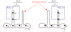
Figure 1: Illustration of a set $X$ and a choice of $\eta$ for which no $\eta$-grid exists: any attempt to cover one “spike” with grid points will result in excluding the other. (Red dashed lines indicate $\eta/2$ balls, and sold circles indicate elements of $X_{\eta}$.)

Now we can state the main theorem of the paper.

Theorem 2 (ReLU Architecture for Control).

Let $\delta>0$, $\tau>0$ and $K_{\text{cont}}>0$ be given, and let $\Sigma$ and $S_{\text{spec}}$ be as in the statement of 2. Furthermore, suppose that there exists a $\delta,\tau$ positively invariant Lipschitz continuous controller $\Psi:\mathbb{R}^{n}\rightarrow U$ with Lipschitz constant $K_{\Psi}\leq K_{\text{cont}}$ such that:

$$S_{\tau}(\Sigma_{\Psi})\preceq_{\mathcal{AD}_{\delta}}S_{\text{spec}}.$$ (23)

Finally, suppose that $\mu>0$ such that:

$$K_{u}\cdot\mu\cdot\tau\cdot e^{(K_{x}+2K_{u}K_{\text{cont}})\tau}<\delta.$$ (24)

If $\eta\leq\frac{\mu}{{3}\cdot K_{\text{cont}}}$ is such that there exists an $\eta$-grid of $X$, then there exists an $m$-fold parallel TLL NN architecture $\text{Arch}(\Theta^{\overset{\text{\tiny TLL}\parallel}{~{}}}_{{}^{n}_{m}\negthinspace N})$ of size (see Corollary 1):

$$N\geq n!\cdot\left\lceil\frac{\text{ext}(X)}{\eta}+2\right\rceil^{n}$$ (25)

with the property that there exist values for $\Theta^{\overset{\text{\tiny TLL}\parallel}{~{}}}_{{}^{n}_{m}\negthinspace N}$ such that:

$$S_{\tau}(\Sigma_{\negthinspace{\scriptstyle{\mathscr{N}\negthickspace\negthickspace\negthinspace\mathscr{N}}\negthinspace\atop~{}}\negthinspace{\Theta^{\overset{\text{\tiny TLL}\parallel}{~{}}}_{{}^{n}_{m}\negthinspace N}}})\preceq_{\mathcal{AD}_{0}}S_{\text{spec}}.$$ (26)

Remark 3.

Note that the coefficient $n!$ in (25) is significantly smaller than the analogous one exhibited in [3]: viz. $\left(n!\cdot\sum_{k=1}^{n}\tfrac{2^{2k-1}}{(n-k)!}\right)$. Furthermore, [3] also failed to account for the need to choose an $\eta$-grid.

The size of the architecture specified by Theorem 2 is effectively determined by the ratio $\text{ext}(X)/\eta$ (for given state and control dimensions). This quantity has two specific connections to the assumptions in 2. On the one hand, the maximum allowable $\eta$ is set by $\mu$, which is determined by the Lipschitz constants of the dynamics and the properties of the assumed controller, $\Psi$. On the other hand, the specific character of state set itself influences the size the architecture, both explicitly by way of $\text{ext}(X)$ and implicitly via the requirement that an $\eta$-grid exists for $X$.

With regard to the first of these influences, (24) can be rearranged to provide the following upper bound for $\eta$:

$$\eta\leq\tfrac{1}{{3}\cdot K_{\text{cont}}\cdot K_{u}}e^{-(K_{x}+2K_{u}K_{\text{cont}})\tau}\cdot\left(\tfrac{\delta}{\tau}\right).$$ (27)

Of unique interest is the influence of the unknown but asserted-to-exist controller, $\Psi$. In particular, note that the robustness of $\Psi$ has an intuitive effect on the size of the architecture. As the robustness of the asserted controller increases (for fixed $\tau$), i.e. as $\delta$ increases, $\eta$ is permitted to be larger, and the architecture can be correspondingly smaller. Of course as the asserted controller becomes less robust, i.e. as $\delta$ decreases, the architecture must correspondingly become larger. This trade off makes intuitive sense in light of our eventual proof strategy: in effect, we will design an architecture that can approximate any potential $\Psi$, so the more robust $\Psi$ is, the less precisely the NN architecture must be able to approximate it – so a smaller architecture suffices (and vice versa). See Section 4.1.

With regard to the second influence, the extent of the set $X$ has a straightforward and direct effect on the designed architecture: the “larger” the set is, the larger the architecture is required. However, the “complexity” of the set $X$ indirectly influences the size of the architecture via the $\eta$-grid requirement. Indeed, if the boundary of $X$ has many thin protuberances (see Fig. 1, for example), then an extremely fine $\eta$ grid may be required to ensure that grid points are placed throughout $X$. Crucially, this choice of $\eta$ may need to be significantly smaller than the maximum allowable $\eta$ computed via (24), as above – the result will be a significantly larger architecture than suggested by (24) alone. Unfortunately, this effect is difficult to quantify directly, given the variability in complexity of state sets. Nevertheless, given any connected compact set $X$, there exists an $\eta>0$ for which $X$ has an $\eta$ grid.

Proposition 1.

Let $X\subset\mathbb{R}^{n}$ be compact and connected with a non-empty interior. Then there exists an $\eta>0$ such that there exists an $\eta$ grid of $X$.

Proof.

We will consider dyadic $\eta$ grids: that is grids based on $\eta_{k}=2^{-k}$, where the associated candidate grid is given by

$$X_{\eta_{k}}\triangleq\{x\in X\;|\;\exists z\in\mathbb{Z}.x=\tfrac{z}{2^{k}}\}.$$ (28)

For convenience, define the following notation:

$$H_{\eta_{k}}\triangleq\cup_{\mathbf{x}\in X_{\eta_{k}}}\overline{B}(\mathbf{x};\eta_{k})$$ (29)

Now because $X$ is connected with non-empty interior, it the case that $\text{bd}(X)=\overline{\text{int}(X)}$. Hence, for every $x\in X$, there exists an $K_{x}$ such that for all $k\geq K_{x}$, $x\in H_{\eta_{k}}$ (consider a truncation of the binary expansion of each coordinate of $x$). It follows that if there is a $K$ such that $K_{x}<K$ for all $x\in X$, then the claim is proved (simply choose $X_{\eta_{K}}$).

Thus, suppose by contradiction that there is a divergent sequence $\{x_{k}\}$ s.t. $K_{x_{k}}<K_{x_{k+1}}$ for all $k\in\mathbb{N}$. However, $X\subset\mathbb{R}^{n}$ is compact, so $\{x_{k}\}$ has a convergent subsequence $\{x_{k_{\ell}}\}$ with limit $x^{\prime}\in X$; this subsequence retains the property that $K_{x_{k_{\ell}}}<K_{x_{k_{\ell+1}}}$. Moreover, by the above claim, there is some $K_{x^{\prime}}$ such that $x^{\prime}\in H_{\eta_{k}}$ for all $k\geq K_{x^{\prime}}$.

Now we consider two cases: first that $x^{\prime}\in B(\mathbf{x};\eta_{K_{x^{\prime}}})$ for some $\mathbf{x}$, and second that $x^{\prime}$ is on the boundary of some $B(\mathbf{x};\eta_{K_{x^{\prime}}})$. In the first case, we note that there exists an $L$ such that for all $\ell\geq L$, $x_{k_{\ell}}\in B(\mathbf{x};\eta_{K_{x^{\prime}}})$, simply by the convergence of the subsequence to $x^{\prime}$. This is clearly a contradiction, since it implies that $x_{k_{\ell}}\in H_{\eta_{K_{x^{\prime}}}}$ for all $\ell\geq L$.

On the other hand, suppose $x^{\prime}$ is on the boundary of some $B(\mathbf{x};\eta_{K_{x^{\prime}}})$, and suppose that $x^{\prime}$ belongs to a $d$-dimensional face of $B(\mathbf{x};\eta_{K_{x^{\prime}}})$ where $1\leq d<n$ (if $d=0$ then $x^{\prime}$ is itself a dyadic point, and the above argument applies directly, since $x^{\prime}\in X_{\eta_{K_{x^{\prime}}}}$). Let this face be denoted $F_{x^{\prime}}$. Then there exists a finite $K_{0}>K_{x^{\prime}}$ such that $x^{\prime}\in B(\mathbf{x};\eta_{K_{0}})$ for some $\mathbf{x}=z/2^{K_{0}}$: use coordinate-wise binary expansions to find a dyadic point within the face $F_{x^{\prime}}$ that includes $x^{\prime}$ in the associated open $\eta_{K}$ ball (this is possible since $F_{x^{\prime}}$ has at least one non-dyadic coordinate by the $d\geq 1$ assumption). This leads to the same contradiction as before, since a tail of the subsequence $\{x_{k_{\ell}}\}$ is eventually contained in this ball. ∎

The remainder of this section is divided as follows. Section 4.1 contains a proof sketch of Theorem 2, which divides the proof into two main intermediate steps. Section 4.2 and Section 4.3 thus contain the formal proofs for these intermediate steps. The overall formal proof of Theorem 2 then appears in Section 4.4.

4.1 Proof Sketch of Theorem 2

Our proof of Theorem 2 implements the following simple strategy. By assumption, a $\Psi$ exists that satisfies the specification robustly (via ADS), and hence, we show that any suitably close approximation of $\Psi$ will function as a controller that satisfies the specification as well (albeit non-robustly). This implies that we need only design a NN architecture with enough parameterization that it can approximate any possible $\Psi$ that satisfies the conditions of the theorem.

There is, however, an important and non-obvious sequence of observations required to design such a NN architecture. To start, any such $\Psi$ is Lipschitz continuous, so it is possible to uniformly approximate it by interpolating between its values taken on a uniform grid. Moreover, its Lipschitz constant has a known upper bound, so for a given approximation accuracy, the fineness of that grid can be chosen conservatively, and hence independent of any particular $\Psi$. However, we show it is possible to interpolate between points over such a uniform grid using a CPWA that has a number of linear regions (Definition 9) proportional to the number of points in the grid – which we reiterate is independent of any particular $\Psi$. This CPWA is in effect parameterized by the values it takes on those grid points, but in such a way that its number of linear regions is independent of those parameter values. This shows that an arbitrary $\Psi$ can be approximated by a CPWA with a fixed number of linear regions; it remains to connect this to a NN architecture. Fortunately, the TLL NN architecture [2] can be used directly for this purpose by way of Theorem 1 [2, Theorem 7]: the result in question explicitly specifies a NN architecture that can implement any CPWA with a known, bounded number of linear regions.

Consequently, the proof of Theorem 2 can instead be decomposed into establishing the following two implications:

1. “Approximate controllers satisfy the specification”: There is a approximation accuracy, $\mu$, and sampling period, $\tau$, with the following property: if the unknown controller $\Psi$ satisfies the specification (under $\delta$ disturbance and sampling period $\tau$), then any controller – NN or otherwise – that approximates $\Psi$ to accuracy $\mu$ in $\lVert\cdot\rVert_{X}$ will also satisfy the specification (but under no disturbance). See Lemma 1.

2. “Any controller can be approximated by a CPWA with the same fixed number of linear regions”: If unknown controller $\Psi$ has a Lipschitz constant $K_{\Psi}\leq K_{\text{cont}}$, then $\Psi$ can be approximated by a CPWA with a number of regions that depends only on $K_{\text{cont}}$ and the approximation accuracy. See Corollary 2.

The conclusion of Theorem 2 then follows from Step 1 and Step 2 by means Theorem 1 [2, Theorem 7], since any CPWA with the same number of linear regions (or fewer) can be implemented exactly by a common TLL NN architecture.

Remark 4.

Unlike our use of Theorem 1 to directly construct a single TLL, the architectures used in [29] consist of two successive TLL layers. The first is used to represent “basis” functions specified over overlapping regular polytopes (decomposable by a common set of simplexes [29, Figure 3.2]); and the second captures the sum of these basis functions. This approach leads to larger architectures compared to our direct approach: consider [29, Eq. (5.3)], which has exponentially many neurons in the number of linear regions. By contrast, the architecture of Theorem 2 has only polynomially many neurons as a function of the number of regions: i.e. as a function of $N$, polynomially many $\min$ units are needed [2], so the $\max$ network has polynomially many neurons; and each $\min$ network is straightforwardly polynomial in $N$.

4.2 Proof of Theorem 2, Step 1: Approximate Controllers Satisfy the Specification

The goal of this section is to choose constant $\mu>0$ such that: for any $\Psi$ satisfying the assumptions in Theorem 2, then any other controller $\Upsilon$ with $\lVert\Upsilon-\Psi\rVert_{X}\leq\mu$ also satisfies the specification, i.e. $S_{\tau}(\Sigma_{\Upsilon})\preceq_{\mathcal{AD}_{0}}S_{\text{spec}}$.

Specifically, we will prove the following lemma.

Lemma 1.

Let $\Sigma$ be as in 2. Also, let $\Psi:X\rightarrow U$ be $\delta$-$\tau$ positively invariant w.r.t $X$, and have Lipschitz constant at most $K_{\text{cont}}$. Further suppose that $\mu>0$ is such that:

$$K_{u}\cdot\mu\cdot\tau\cdot e^{(K_{x}+K_{u}K_{\Upsilon})\tau}<\delta.$$ (30)

Then for any $\Upsilon:\mathbb{R}^{n}\rightarrow\mathbb{R}^{m}$ that is Lipschitz continuous with Lipschitz constant $K_{\Upsilon}$, we have that

$$\lVert\Upsilon-\Psi\rVert_{X}\leq\mu\implies S_{\tau}(\Sigma_{\Upsilon})\preceq_{\mathcal{AD}_{0}}\mathfrak{S}_{\tau}(\Sigma_{\Psi}).$$ (31)

And hence if in addition $S_{\tau}(\Sigma_{\Psi})\preceq_{\mathcal{AD}_{\delta}}S_{\text{spec}}$, then:

$$S_{\tau}(\Sigma_{\Upsilon})\preceq_{\mathcal{AD}_{0}}S_{\text{spec}}.$$ (32)

Our specific approach to prove this will be as follows. First, we choose $\mu$ small enough such that a $\tau$-second flow of $\zeta_{x\Upsilon}$ doesn’t deviate by more that $\delta$ from $\zeta_{x\Psi}$ over its duration, $\tau$. This is accomplished by means of a Grönwall-type bound that uses $\lVert\Upsilon-\Psi\rVert_{X}<\mu$. That is assume $\Psi$ is $\delta$-$\tau$ positively invariant, and use $\lVert\Upsilon-\Psi\rVert_{X}\leq\mu$ in the Grönwall inequality:

$$\forall x\in X.\lVert\zeta_{x\Upsilon}(\tau)-\zeta_{x\Psi}(\tau)\rVert\leq K_{u}\cdot\mu\cdot\tau\cdot e^{(K_{x}+K_{u}K_{\Upsilon})\tau}\negthinspace\negthinspace<\negthinspace\delta.$$ (33)

Then we use this conclusion to construct the appropriate simulation relations that show:

$$S_{\tau}(\Sigma_{\Upsilon})\preceq_{\mathcal{AD}_{0}}\mathfrak{S}_{\tau}(\Sigma_{\Psi})\preceq_{\mathcal{AD}_{0}}S_{\text{spec}}.$$ (34)

First, we formally obtain the desired conclusion of (33) by way of the following proposition.

Proposition 2.

Let $\Sigma$ and $\Psi$ be as in the statement of Lemma 1, and let $\Upsilon:\mathbb{R}^{n}\rightarrow\mathbb{R}^{m}$ be Lipschitz continuous with Lipschitz constant $K_{\Upsilon}$. Also, suppose that $\mu>0$ is such that:

$$K_{u}\cdot\mu\cdot\tau\cdot e^{(K_{x}+K_{u}K_{\Upsilon})\tau}<\delta.$$ (35)

If $\lVert\Upsilon-\Psi\rVert_{X}\leq\mu$, then for any $x\in X$:

$$\lVert\zeta_{x\Upsilon}(\tau)-\zeta_{x\Psi}(\tau)\rVert\leq\delta.$$ (36)

Proof.

By definition,we have:

$$\lVert\zeta_{x\Upsilon}(t)-\zeta_{x\Psi}(t)\rVert$$

$$\negthinspace\negthinspace\leq\negthinspace\negthinspace\negthinspace\int_{0}^{t}\lVert f(\zeta_{x\Upsilon}(\sigma),\Upsilon(\zeta_{x\Upsilon}(\sigma)))-f(\zeta_{x\Psi}(t),\Psi^{\prime}(\zeta_{x\Psi}(t)))\rVert d\sigma$$

$$\negthinspace\negthinspace\leq\negthinspace\negthinspace\negthinspace\int_{0}^{t}\negthinspace\negthinspace\negthinspace\negthinspace K_{x}\lVert\zeta_{x\Upsilon}(\sigma)-\zeta_{x\Psi}(\sigma)\rVert+K_{u}\lVert\Upsilon(\zeta_{x\Upsilon}(\sigma))-\Psi(\zeta_{x\Psi}(\sigma))\rVert d\sigma$$ (37)

Now, we consider bounding the second normed quantity in (37). In particular, we have that:

$$\lVert\Upsilon(\zeta_{x\Upsilon}(\sigma))-\Psi(\zeta_{x\Psi}(\sigma))\rVert$$

$$\;\leq\lVert\Upsilon(\zeta_{x\Upsilon}(\sigma))-\Upsilon(\zeta_{x\Psi}(\sigma))\rVert+\lVert\Upsilon(\zeta_{x\Psi}(\sigma))-\Psi(\zeta_{x\Psi}(\sigma))\rVert$$

$$\;\leq K_{\Upsilon}\cdot\lVert\zeta_{x\Upsilon}(\sigma)-\zeta_{x\Psi}(\sigma)\rVert+\lVert\Upsilon-\Psi\rVert_{X}.$$ (38)

The first term is so bounded because $\Upsilon$ is assumed to be globally Lipschitz continuous on all of $\mathbb{R}^{n}$. In particular, the first term of (38) can be bounded using the global Lipschitz continuity of $\Upsilon$, whether $\zeta_{x\Upsilon}(t)$ lies in $X$ or not. The second term is bounded as claimed because $\zeta_{x\Psi}(t)\in X$ for all $t$ by the assumption of ($\delta$-$\tau$) forward invariance of $\Psi$: consequently, the $X$-restricted $\sup$ norm may be employed.

Thus, using (37) and (38), we obtain the bound

$$\lVert\zeta_{x\Upsilon}(t)-\zeta_{x\Psi}(t)\rVert\leq\negthinspace\int_{0}^{t}\negthinspace(K_{x}+K_{u}K_{\Upsilon})\negthinspace\cdot\negthinspace\lVert\zeta_{x\Upsilon}(\sigma)-\zeta_{x\Psi}(\sigma)\rVert$$

$$\qquad\qquad\qquad\qquad\qquad\qquad+K_{u}\cdot\lVert\Upsilon-\Psi\rVert_{X}d\sigma.$$ (39)

where the second term of the integrand is bounded by the constant $K_{u}\cdot\mu$ by assumption. The claimed bound now follows from (39) by the Grönwall Inequality [30]. ∎

Now we can prove the main result of this section, Lemma 1; this proof follows more or less directly from Proposition 2.

Proof.

(Lemma 1) By definition, $S_{\tau}(\Sigma_{\Upsilon})$ and $\mathfrak{S}_{\tau}(\Sigma_{\Psi})$ have the same state spaces, $X$. Thus, we propose the following as an abstract disturbance simulation under $0$ disturbance (i.e. a conventional simulation for metric transition systems):

$$R=\{(x,x)|x\in X\}.$$ (40)

Clearly, $R$ satisfies the property that for all $(x,y)\in R$, $d(x,y)\leq 0$, and for every $x\in X$, there exists an $y\in X$ such that $(x,y)\in R$. Thus, it only remains to show the third property of Definition 13 under $0$ disturbance.

To wit, let $(x,x)\in R$. Then suppose that $x^{\prime}\triangleq\zeta_{x\Upsilon}(\tau)\in X$, so that $x\overset{\Upsilon\circ\zeta_{x\Upsilon}}{{}_{\scriptscriptstyle\Sigma_{\Upsilon}}\negthickspace\negthickspace\negthinspace\negthinspace\longrightarrow}x^{\prime}$ in $S_{\tau}(\Sigma_{\Upsilon})$; we will show subsequently that any such $x^{\prime}$ must be in $X$. In this situation, it suffices to show that $x\overset{\Psi\circ\zeta_{x\Psi}}{{}_{\scriptscriptstyle\Sigma_{\Psi}}\negthickspace\negthickspace\negthinspace\negthinspace\longrightarrow}x^{\prime}$ in $\mathfrak{S}_{\tau}(\Sigma_{\Psi})$. By the $\delta,\tau$ positive invariance of $\Psi$, it is the case that $x^{\prime\prime}\triangleq\zeta_{x\Psi}(\tau)\in X\backslash\text{edge}_{\delta}(X)$, so $x\overset{\Psi\circ\zeta_{x\Psi}}{{}_{\scriptscriptstyle\Sigma_{\Psi}}\negthickspace\negthickspace\negthinspace\negthinspace\longrightarrow}x^{\prime\prime}$ in $S_{\tau}(\Sigma_{\Psi})$. But by Proposition 2, $\lVert x^{\prime}-x^{\prime\prime}\rVert\leq\delta$, so $x\overset{\Psi\circ\zeta_{x\Psi}}{{}_{\scriptscriptstyle\Sigma_{\Psi}}\negthickspace\negthickspace\negthinspace\negthinspace\longrightarrow}x^{\prime}$ in $\mathfrak{S}_{\tau}(\Sigma_{\Psi})$ by definition.

It remains to show that any such $x^{\prime}\triangleq\zeta_{x\Upsilon}(\tau)\in X$. This follows by contradiction from Proposition 2 and the $\delta,\tau$ positive invariance of $\Psi$. That is suppose $x^{\prime}\notin X$. By Proposition 2, $x^{\prime\prime}\triangleq\zeta_{x\Psi}(\tau)$ satisfies $\lVert x^{\prime}-x^{\prime\prime}\rVert\leq\delta$, which implies that $x^{\prime\prime}\in\text{edge}_{\delta}(X)\cup\mathbb{R}^{n}\backslash X$. However, this clearly contradicts the $\delta,\tau$ positive invariance of $\Psi$. ∎

4.3 Proof of Theorem 2, Step 2: CPWA Approximation of a Controller

The results in Section 4.2 established a choice of $\mu$ such that any controller, $\Upsilon$, whether it is CPWA or not, will satisfy the specification if it is close to $\Psi$ in the sense that $\lVert\Upsilon-\Psi\rVert_{X}\leq\mu$; that is, provided $\Psi$ itself satisfies the specification by $\delta$-ADS for the chosen $\tau$. In other words, if such a $\Psi$ were explicitly known, then a CPWA controller, $\Upsilon_{\negthinspace\text{\tiny CPWA}}$, that meets this approximation criterion would also be a safe controller. In such a circumstance, that explicit CPWA controller could be implemented as a ReLU by way of Theorem 1, and the architecture of that ReLU controller would suffice as an assured controller architecture.

However, we have assumed ignorance of a specific such $\Psi$, so we instead have to devise an architecture that can approximate any such possible $\Psi$ that meets the specifications. Thus, we create a parameterized CPWA that can achieve the desired approximation accuracy of $\mu$ for any possible $\Psi$ merely by a choice of parameters. Moreover, this parameterized CPWA must have a bounded number of linear regions in order to obtain a ReLU architecture by Theorem 1. Both of these objectives will prove feasible because we have assumed that any $\Psi$ has a Lipschitz constant that is upper-bounded by the known constant $K_{\text{cont}}$. Indeed, our parameterized CPWA will have as parameters the values of $\Psi$ on a uniformly spaced set of points in $X$; we will show that these function evaluations can be interpolated by a CPWA with a number of linear regions proportional to the number of grid points.

The mechanism for obtaining such a CPWA interpolation will ultimately be to “tile” the set $X\subset\mathbb{R}^{n}$ by $n$-simplexes, each of whose vertices are points from the interpolation grid. That is, we will choose these simplexes such that a full-dimensional face of any simplex will be shared exactly by one and only one other simplex. Each simplex can then be regarded as corresponding to a linear region, because the graph of (any) $\Psi$ on its $n+1$ vertices defines an affine function over that simplex. Moreover, an affine function on one simplex is continuous with the affine function defined on any of its neighbors, because of the face-sharing property described above. Thus, this approach constructs an interpolation CPWA where each affine function is “activated” only on its respective simplex. Crucially, this construction leads to a CPWA with same number of linear regions, irrespective of the particular values of $\Psi$: the number of simplexes is determined entirely by the spacing of the uniform grid, which is in turn determined only by Lipschitz constants and the set $X$ itself. Hence, the grid can be specified by the problem parameters, and the values of $\Psi$ thereon can be considered as parameters. This is exactly a parameterized CPWA of the sort described above; the culmination of this approach is in Corollary 2.

4.3.1 Preliminaries

Before we state the main result of this section, we introduce the following notation to refer to those hypercubes that have at least one corner in $X_{\eta}$, but no elements of $X_{\eta}$ in their interior.

Definition 16 (Interpolation Hypercube).

Let $X_{\eta}$ be an $\eta$-grid of $X$, and let $\mathbf{x}\in X_{\eta}$. Then each vector $\rho\in\{-1,1\}^{n}$ defines an interpolation hypercube relative to $\mathbf{x}_{i}$ given by:

$$C_{\mathbf{x}\rho}\triangleq B(\mathbf{x}+\tfrac{\eta}{2}\cdot{\scriptstyle\sum_{i=1}^{n}}\pi_{i}(\rho)\cdot e_{j})$$ (41)

and whose corners are

$$\mathscr{F}_{0}(C_{\mathbf{x}\rho})=\{\mathbf{x}+\eta\cdot\sum_{i\in Z}\pi_{i}(\rho)\cdot e_{i}|Z\subseteq\{1,\dots,n\}\},$$ (42)

where $e_{i}$ is the $i^{\text{th}}$ column of the $(n\times n)$ identity matrix.

Note that $\cup_{\rho\in\{-1,1\}^{n}}C_{\mathbf{x}\rho}=B(\mathbf{x};\eta)$. Fig. 3 is a cartoon that depicts interpolation hypercubes, among other things.

Interpolation hypercubes can have corners that lie outside of $X$, and we will subsequently need to treat these corners separately. Hence the following notation for an extra corner.

Definition 17 (Extra Corner).

Let $C_{\mathbf{x}\rho}$ be an interpolation hypercube of an $\eta$-grid, $X_{\eta}$. Then an extra corner of $C_{\mathbf{x}\rho}$ is any corner $x\in\mathscr{F}_{0}(C_{\mathbf{x}\rho})\backslash X_{\eta}$. Denote the set of all extra corners of all interpolation hypercubes of $X_{\eta}$ as

$$\Delta_{X_{\eta}}\triangleq\bigcup_{\mathbf{x}\in X_{\eta}}\mathscr{F}_{0}(C_{\mathbf{x}\rho})\backslash X_{\eta}.$$ (43)

Finally, we have the following proposition, which indicates the maximum number of interpolation hypercubes that are required to cover $X$ (by tiling), given an $\eta$-grid, $X_{\eta}$.

Proposition 3.

Let $X_{\eta}$ be an $\eta$ grid for $X$ as before. Then $X$ is covered by the union of at most

$$\left\lceil\frac{\text{ext}(X)}{\eta}+2\right\rceil^{n}$$ (44)

interpolation hypercubes.

Proof.

A compact set $X$ can be contained in a hypercube with edge-length $\text{ext}(X)$, which can in turn be partitioned by at most $\lceil\text{ext}(X)/\eta\rceil^{n}$ elements. Thus, $|X_{\eta}|\leq\lceil\text{ext}(X)/\eta\rceil^{n}$. It follows then that $X$ can be covered by the inclusion of one interpolation hypercube per element of $X_{\eta}$, plus one extra set of interpolation hypercubes at either extreme of each coordinate. ∎

Remark 5.

Note that an $\eta$-grid of $X$ effectively specifies a tiling of no more than (44) hypercubes covering $X$: i.e. the interpolation hypercubes cover $X$, and a full dimensional face of any one of them is shared by one and only one other interpolation hypercube.

4.3.2 Parameterized CPWA for Approximation

Now we can state the main results of this section. The first, Lemma 2, specifies the structure and properties of the parameterized CPWA that we will use. Thus, as a corollary, we have Corollary 2, which particularizes this parameterized CPWA to Step 2 in the proof of Theorem 2.

Lemma 2.

Let $\eta>0$ be fixed, and let $X$ be compact. Also let $X_{\eta}$ be an $\eta$-grid of $X$ that is enumerated as $X_{\eta}=\{\mathbf{x}_{i}\}_{i=0}^{|X_{\eta}|-1}$.

Then there is a parameterized CPWA $\Upsilon_{\omega}:X\rightarrow\mathbb{R}$ with parameter vector $\omega\in\mathbb{R}^{|X_{\eta}|}$ that has the following properties:

1. for all $i=0,\dots|X_{\eta}|-1$ and $j=0,\dots,n-1$,

   $$\pi_{i}(\omega)=\Upsilon_{\omega}(\mathbf{x}_{i});$$ (45)

   i.e. $\omega$ specifies the value of $\Upsilon_{\omega}$ on the grid $X_{\eta}$;

2. $\Upsilon_{\omega}$ has at most

   $$n!\cdot\left\lceil\frac{\text{ext}(X)}{\eta}+2\right\rceil^{n}$$ (46)

   linear regions no matter the value of $\omega$; and

3. let $\nu_{\mathbf{x}_{i}\rho}\triangleq\cup_{x\in\mathscr{F}_{0}(C_{\mathbf{x}_{i}\rho})}B(x;\eta)$; then for each interpolation hypercube $C_{\mathbf{x}_{i}\rho}$ of $X_{\eta}$ and each $x\in C_{\mathbf{x}_{i}\rho}$,

   $$\min_{\mathbf{x}^{\prime}\in\nu_{\mathbf{x}_{i}\rho}\cap X_{\eta}}\negthickspace\negthickspace\Upsilon_{\omega}(\mathbf{x}^{\prime})\leq\Upsilon_{\omega}(x)\leq\negthickspace\max_{\mathbf{x}^{\prime}\in\nu_{\mathbf{x}_{i}\rho}\cap X_{\eta}}\negthickspace\negthickspace\Upsilon_{\omega}(\mathbf{x}^{\prime}).$$ (47)

We defer the proof of Lemma 2 to Section 4.3.3 in order to immediately state the conclusion of relevance for Step 2 in the proof of Theorem 2.

Corollary 2.

Let $K_{\text{cont}}>0$ be given, and let $\mu>0$ and $\eta\leq\tfrac{\mu}{{3}\cdot K_{\text{cont}}}$ be as above. Also let $\Psi:X\rightarrow U$ be any Lipschitz continuous function with Lipschitz constant at most $K_{\text{cont}}$.

If we use the parameterized CPWA from Lemma 2 component-wise, with the $j^{\text{th}}$ parameter vector specified by

$$\omega^{(j)}=\omega_{\Psi}^{(j)}\triangleq\prod_{i=0}^{|X_{\eta}|-1}\{\pi_{j}(\Psi(\mathbf{x}_{i}))\},$$ (48)

then $\Upsilon_{\omega_{\Psi}}\triangleq\left(\begin{smallmatrix}\Upsilon_{\omega_{\Psi}^{(1)}}&\dots&\Upsilon_{\omega_{\Psi}^{(m)}}\end{smallmatrix}\right)$ agrees with $\Psi$ on $X_{\eta}$ and

$$\lVert\Upsilon_{\omega_{\Psi}}-\Psi\rVert_{X}\leq\mu.$$ (49)

Moreover, $\Upsilon_{\omega_{\Psi}}$ has at most $n!\cdot\lceil\text{ext}(X)/\eta+2\rceil^{n}$ linear regions for each component-wise function, independent of the particular choice of $\Psi$. Finally, $\Upsilon_{\omega_{\Psi}}$ has a Lipschitz constant of at most ${3}\cdot K_{\Psi}$ on $\bigcup_{\mathbf{x}\in X_{\eta},\rho\in\{-1,1\}^{n}}C_{\mathbf{x}\rho}\supseteq X$.

Proof.

This follows from Lemma 2, with the exception of (49), and the claim about the Lipschitz constant of $\Upsilon_{\omega_{\Psi}}$.

The claim (49) follows from (47) in Lemma 2, given that $\eta$ was assumed chosen as $\eta\leq\tfrac{\mu}{{3}K_{\text{cont}}}$. In particular, we have that for any interpolation hypercube $C_{\mathbf{x}_{i}\rho}$ and any $x\in C_{\mathbf{x}_{i}\rho}$, there exists a $j\in\{1,\dots,m\}$ s.t.

$$\lVert\Upsilon_{\omega_{\Psi}}(x)-\Psi(x)\rVert=|\pi_{j}(\Psi(x))-\Upsilon_{\omega_{\Psi}^{(j)}}(x)|$$ (50)

From here, we consider as separate cases both possible signs of $\pi_{j}(\Psi(x))-\Upsilon_{\omega_{\Psi}^{(j)}}(x)$. However, for brevity, we write out only the case $\pi_{j}(\Psi(x))-\Upsilon_{\omega_{\Psi}^{(j)}}(x)\geq 0$, since the other case can be treated by similar arguments. In this case:

$$\lVert\Upsilon_{\omega_{\Psi}}(x)-\Psi(x)\rVert =|\pi_{j}(\Psi(x))-\Upsilon_{\omega_{\Psi}^{(j)}}(x)|$$

$$=\pi_{j}(\Psi(x))-\Upsilon_{\omega_{\Psi}^{(j)}}(x)$$

$$\leq\pi_{j}(\Psi(x))-\negthickspace\negthickspace\negthinspace\min_{\mathbf{x}^{\prime}\in\nu_{\mathbf{x}_{i}\rho}\cap X_{\eta}}\negthickspace\negthickspace\Upsilon_{\omega_{\Psi}^{(j)}}(\mathbf{x}^{\prime})$$ (51)

where the (51) follows from Lemma 2, equation (47). Then we note that there exists an $\mathbf{x}\in\nu_{\mathbf{x}_{i}\rho}\cap X_{\eta}$ such that

$$\min_{\mathbf{x}^{\prime}\in\nu_{\mathbf{x}_{i}\rho}\cap X_{\eta}}\negthickspace\negthickspace\Upsilon_{\omega_{\Psi}^{(j)}}(\mathbf{x}^{\prime})=\Upsilon_{\omega_{\Psi}^{(j)}}(\mathbf{x})=\pi_{j}(\Psi(\mathbf{x}))$$ (52)

by i) of Lemma 2. But by construction, $\mathbf{x}\in\nu_{\mathbf{x}_{i}\rho}$, so there exists an $x^{\prime\prime}\in\mathscr{F}_{0}(C_{\mathbf{x}_{i}\rho})$ such that $\mathbf{x}\in B(x^{\prime\prime};\eta)$. It follows that $\lVert x-\mathbf{x}\rVert\leq\lVert x-x^{\prime\prime}\rVert+\lVert x^{\prime\prime}-\mathbf{x}\rVert\leq 2\eta$. Thus, by the choice of $\eta\leq\tfrac{\mu}{{3}K_{\text{cont}}}$, $K_{\text{cont}}$-Lipschitz continuity of $\Psi$ implies:

$$\lVert\Upsilon_{\omega_{\Psi}}(x)-\Psi(x)\rVert \leq\pi_{j}(\Psi(x))-\pi_{j}(\Psi(\mathbf{x}))$$

$$\leq\lVert\Psi(x)-\Psi(\mathbf{x})\rVert\leq\tfrac{2}{3}\mu\leq\mu$$ (53)

This concludes the proof for the case $\pi_{j}(\Psi(x))-\pi_{j}(\Upsilon_{\omega_{\Psi}^{(j)}}(x))\geq 0$; the other case follows similarly.

Thus, it remains to show the claim about the Lipschitz constant of $\Upsilon_{\omega_{\Psi}}$. This ultimately follows from the observation that every affine function in $\Upsilon_{\omega_{\Psi}}$ interpolates between the values specified on the corners of some interpolation hypercube. Consequently, it suffices to show that the Lipschitz constant of none of these affine functions exceeds the claimed value. Thus, let $x,x^{\prime}\in C_{\mathbf{x}\rho}$ be arbitrary such that $x$ and $x^{\prime}$ belong to the same simplex of the dissection $\mathcal{D}_{\mathcal{B}_{n}}$ (see Lemma 4). Now by linear interpolation between the values of $\Upsilon_{\omega_{\Psi}}$ on that simplex, there exists for each coordinate $i=1,\dots,m$ a pair of corners $x_{\min}^{i},x_{\max}^{i}\in\mathscr{F}_{0}(C_{\mathbf{x}\rho})$ such that

$$\pi_{i}(\Upsilon_{\omega_{\Psi}}(x_{\min}^{i}))\leq\pi_{i}(\Upsilon_{\omega_{\Psi}}(x))\leq\pi_{i}(\Upsilon_{\omega_{\Psi}}(x_{\max}^{i})),$$ (54)

and which holds for any $x$ in the same simplex. Now define:

$$y_{\Delta} \triangleq\max_{i}\left[\pi_{i}(\Upsilon_{\omega_{\Psi}}(x_{\max}^{i}))-\pi_{i}(\Upsilon_{\omega_{\Psi}}(x_{\min}^{i}))\right];\text{ and}$$ (55)

$$\mathsf{i}_{\Delta} \triangleq\arg\max_{i}\left[\pi_{i}(\Upsilon_{\omega_{\Psi}}(x_{\max}^{i}))-\pi_{i}(\Upsilon_{\omega_{\Psi}}(x_{\min}^{i}))\right]$$ (56)

Assuming without loss of generality that $y_{\Delta}\neq 0$, then by linearity of $\Upsilon_{\omega_{\Psi}}$ on the simplex containing $x$ and $x^{\prime}$:

$$\lVert\Upsilon_{\omega_{\Psi}}(x)-\Upsilon_{\omega_{\Psi}}(x^{\prime})\rVert\leq\frac{y_{\Delta}}{\eta}\lVert x-x^{\prime}\rVert$$ (57)

assuming $x_{\min}^{\mathsf{i}_{\Delta}}$ and $x_{\max}^{\mathsf{i}_{\Delta}}$ are achieved on the closest corners of $C_{\mathbf{x}\rho}$, and $x-x^{\prime}$ defines a line parallel to the ${\mathsf{i}_{\Delta}}^{\text{th}}$ coordinate.

On the other hand, we note that

$$y_{\Delta} =\pi_{\mathsf{i}_{\Delta}}(\Upsilon_{\omega_{\Psi}}(x_{\max}^{\mathsf{i}_{\Delta}})-\Upsilon_{\omega_{\Psi}}(x_{\min}^{\mathsf{i}_{\Delta}}))$$

$$=\pi_{\mathsf{i}_{\Delta}}(|\Upsilon_{\omega_{\Psi}}(x_{\max}^{\mathsf{i}_{\Delta}})-\Upsilon_{\omega_{\Psi}}(x_{\min}^{\mathsf{i}_{\Delta}})|)$$

$$\leq\lVert\Upsilon_{\omega_{\Psi}}(x_{\max}^{\mathsf{i}_{\Delta}})-\Upsilon_{\omega_{\Psi}}(x_{\min}^{\mathsf{i}_{\Delta}})\rVert.$$ (58)

Now note that the value of $\Upsilon_{\omega_{\Psi}}$ on $x_{\min}^{\mathsf{i}_{\Delta}}$ and $x_{\max}^{\mathsf{i}_{\Delta}}$ is specified as the value of $\Psi$ on some $\eta$-grid points no further than $\eta$ away from each of those corners; recall the use of $\nu_{\mathbf{x}_{i}\rho}$ in the statement of Lemma 2, iii). In particular, this implies that

$$\exists\mathbf{x}_{\min}\in X_{\eta}\;.\;\lVert x_{\min}^{\mathsf{i}_{\Delta}}-\mathbf{x}_{\min}\rVert\leq\eta\wedge\Upsilon_{\omega_{\Psi}}(x_{\min}^{\mathsf{i}_{\Delta}})=\Psi(\mathbf{x}_{\min})$$ (59)

and likewise for $\mathbf{x}_{\max}$. Thus, we have the following:

$$\lVert\Upsilon_{\omega_{\Psi}}(x_{\max}^{\mathsf{i}_{\Delta}})-\Upsilon_{\omega_{\Psi}}(x_{\min}^{\mathsf{i}_{\Delta}})\rVert =\lVert\Psi(\mathbf{x}_{\max})-\Psi(\mathbf{x}_{\min})\rVert$$

$$\leq K_{\Psi}\cdot\lVert\mathbf{x}_{\max}-\mathbf{x}_{\min}\rVert$$

$$\leq K_{\Psi}\cdot{3}\cdot\eta$$ (60)

which follow by Lipschitz continuity of $\Psi$. Substituting (60) into (57) gives the bound on the Lipschitz constant of $\Upsilon_{\omega_{\Psi}}$ ∎

4.3.3 Proof of Lemma 2

Our approach to proving Lemma 2 will be as follows. On the domain $X_{\eta}$, we will first define a function $\Gamma_{\omega}:X_{\eta}\rightarrow\mathbb{R}$ as $\Gamma_{\omega}:\mathbf{x}_{i}\mapsto\pi_{i}(\omega)$. Then we will extend $\Gamma_{\omega}$ as a CPWA to the union of all of the interpolation hypercubes of $X_{\eta}$, i.e. $\bigcup_{\mathbf{x}\in X_{\eta},\rho\in\{-1,1\}^{n}}C_{\mathbf{x}\rho}$. By this means, we obtain a parameterized CPWA that satisfies Lemma 2.

To accomplish this, we will first need to consider the problem of extending $\Gamma_{\omega}$ from the corners of a specific interpolation hypercube to the rest of that interpolation hypercube itself. Importantly, however, this interpolation must be systematized in such a way that adjacent interpolation hypercubes have consistent interpolations on the non-trivial faces they have in common. Thus, we have the following two generic lemmas, which are the last facilitators we will need in order to prove Lemma 2. Lemma 3 describes the general methodology we undertake for doing this: namely, dividing the hypercube into simplexes, each of which represents a linear region in the CPWA. Lemma 4 then considers a particular instance of this construction that has several unique properties; in particular, it is a consequence of Lemma 4 that will permit a globally consistent interpolation despite considering each interpolation hypercube individually.

Lemma 3.

Let $C_{n}=[0,1]^{n}$, and suppose that:

$$\alpha:\mathscr{F}_{0}(C_{n})\rightarrow\mathbb{R}$$ (61)

is a function defined on the corners of $C_{n}$. Also suppose that $\mathcal{D}=\{\mathsf{s}_{i}\}_{i=1}^{N_{\mathcal{D}}}$ is a set of $n$-simplexes such that: their vertices are contained in $\mathscr{F}_{0}(C_{n})$; they together partition $C_{n}$; and any non-trivial face of one simplex is shared exactly by one and only one other simplex. $\mathcal{D}$ is thus a special case of a dissection of $C_{n}$.

Then $\mathcal{D}$ induces a uniquely defined CPWA function $\Xi_{\alpha}^{\mathcal{D}}:C_{n}\rightarrow\mathbb{R}$ such that:

1. $\forall x\in\mathscr{F}_{0}(C).\Xi_{\alpha}^{\mathcal{D}}\negthinspace(x)=\alpha(x)$, i.e. $\Xi_{\alpha}^{\mathcal{D}}$ extends $\alpha$ to $C$; and

2. for all $x\in C$,

   $$\min_{x\in\mathscr{F}_{0}(C)}\alpha(x)\leq\Xi_{\alpha}^{\mathcal{D}}\negthinspace(x)\leq\max_{x\in\mathscr{F}_{0}(C)}\alpha(x).$$ (62)

Proof.

This follows because each such simplex specifies $n+1$ points from $\text{graph}(\alpha)$, so there is at least one hyperplane that interpolates between those points in $\mathbb{R}^{n+1}$.

In particular, let $V_{\mathsf{s}_{i}}$ be the vertices of the simplex $\mathsf{s}_{i}\in\mathcal{D}$. By assumption, $V_{\mathsf{s}_{i}}\subset\mathscr{F}_{0}(C_{n})$, so $\alpha$ is defined on $V_{\mathsf{s}_{i}}$ for each $\mathsf{s}_{i}$. Thus, let $G_{i}\triangleq\{(v,\alpha(v))\in\mathbb{R}^{n+1}|v\in V_{\mathsf{s}_{i}}\}\subset\text{graph}(\alpha)$ with $G_{i}$ enumerated as $G_{i}=\{g_{i,j}\}_{j=1}^{n+1}$. Then $\mathsf{s}_{i}$ defines at least one hyperplane in $\mathbb{R}^{n+1}$ specified by

$$h_{i}:x\in\mathbb{R}^{n+1}\mapsto\left(\begin{smallmatrix}w_{i}\\ 1\end{smallmatrix}\right)^{\text{T}}(x-b_{i})+b_{i}$$ (63)

where $b_{i}\triangleq\tfrac{1}{n+1}\sum_{g\in G_{i}}g$ and $w_{i}\in\mathbb{R}^{n}$ solves the following (assuming without loss of generality that $\alpha$ has distinct values):

$$\left(\begin{matrix}g_{i,1}\negthinspace-\negthinspace b_{i}&\dots&g_{i,n+1}\negthinspace-\negthinspace b_{i}\end{matrix}\right)^{\text{T}}\left(\begin{smallmatrix}w_{i}\\ 1\end{smallmatrix}\right)=0.$$ (64)

Consequently, each hyperplane, $h_{i}$, defines an affine function on $\mathbb{R}^{n}$ that interpolates $\alpha$ between the relevant points in its domain (the vertices of its simplex). That is the graph of

$$a_{i}:x\in\mathbb{R}^{n}\mapsto w_{i}^{\text{T}}x-\left(\begin{smallmatrix}w_{i}\\ 1\end{smallmatrix}\right)b_{i}+b_{i}$$ (65)

contains $G_{i}\subset\text{graph}(\alpha)$. It also follows that

$$\forall x\in\mathsf{s}_{i}\;.\;\min_{v\in V_{\mathsf{s}_{i}}}\alpha(v)\leq a_{i}(x)\leq\max_{v\in V_{\mathsf{s}_{i}}}\alpha(v),$$ (66)

since $a_{i}$ linearly interpolates between the points $G_{i}$.

Moreover, any two such affine functions (hyperplanes) necessarily agree on any non-trivial face shared by their respective simplexes. To see this, let $\hat{G}_{i,i^{\prime}}\triangleq G_{i}\cap G_{i^{\prime}}\neq\emptyset$ be the vertices of such a shared face. Then for all $x\in\text{hull}(\hat{G}_{i,i^{\prime}})$, we have $h_{i}(x)=0=h_{i^{\prime}}(x)$. But from the form of (63), the coefficient of the $n+1^{\text{th}}$ coordinate of $x$ is one for both $h_{i}$ and $h_{i^{\prime}}$. Hence we conclude that for all $x\in\mathbb{R}^{n}$ and $y\in\mathbb{R}$

$$\left(\begin{smallmatrix}x\\ y\end{smallmatrix}\right)\in\text{hull}(\hat{G}_{i,i^{\prime}})\implies a_{i}(x)=y=a_{i^{\prime}}(x).$$ (67)

Thus $a_{i}=a_{i^{\prime}}$ on $\text{hull}(V_{\mathsf{s}_{i}})\cap\text{hull}(V_{\mathsf{s}_{i^{\prime}}})$, the face $\mathsf{s}_{i}$ and $\mathsf{s}_{i^{\prime}}$ share.

Hence, we can define a piecewise-affine function:

$$\Xi_{\alpha}^{\mathcal{D}}:x\in C_{n}\mapsto\begin{cases}a_{i}(x)&\text{if }x\in\mathsf{s}_{i}\end{cases}$$ (68)

with the assurance that it is a continuous function on $C_{n}$ by the argument above. Of course this CPWA trivially satisfies ii) in the statement of the lemma by construction. ∎

Thus, to obtain interpolate between such an $\alpha$ it suffices to construct a dissection of $C_{n}$ with the properties assumed in Lemma 3. However, to prove Lemma 2, we use a particular dissection in order to get a suitable CPWA extension; specifically, we need to consider how these CPWA extensions interact on adjacent interpolation hypercubes, whence ii) below.

Lemma 4.

Let $C=[0,1]^{n}$, and suppose that:

$$\alpha:\mathscr{F}_{0}(C_{n})\rightarrow\mathbb{R}$$ (69)

is a function defined on the corners of $C_{n}$.

Also, define $n\cdot(n-1)/2$ hyperplanes from the equations $b_{ij}(x)=0$, $i=1,\dots,n;j<i$, where the $b_{ij}$ are given by:

$$\left.\begin{matrix}b_{ij}:\mathbb{R}^{n}\rightarrow\mathbb{R}\hphantom{12345678\;}\\ b_{ij}:x\mapsto\pi_{i}(x)-\pi_{j}(x)\end{matrix}\right\}\;\text{ for }\;\begin{matrix}i\in\{1,\dots,n\}\\ j<i\hphantom{\qquad 1234}\end{matrix}$$ (70)

so that $\mathcal{B}_{n}\triangleq\{b_{ij}\}_{i\in\{1\dots n\};j<i}$ is the so-called braid arrangement of hyperplanes [36]. Furthermore, let

$$\mathcal{D}_{\mathcal{B}_{n}}\triangleq\{\overline{R\cap\text{int}(C_{n})}|R\text{ is a region in }\mathcal{B}\}$$ (71)

be the dissection of $C_{n}$ by the regions of $\mathcal{B}$.

Then $\mathcal{D}_{\mathcal{B}_{n}}$ is a dissection of $C_{n}$ by $n$-simplexes, each of which has vertices only in $\mathscr{F}_{0}(C_{n})$. Thus, Lemma 3 applies, and the resultant interpolation, $\Xi_{\alpha}^{\mathcal{B}_{n}}$, has further properties:

1. $\Xi_{\alpha}^{\mathcal{B}_{n}}$ has at most $n!$ linear regions in $C_{n}$;

2. for any $n-1$-dimensional face $F_{i}^{k}\in\mathscr{F}_{n-1}(C_{n})$ (as in Definition 11) and any other function $\alpha^{\prime}:\mathscr{F}_{0}(C_{n})\rightarrow\mathbb{R}$ we have that

   $$\forall x\in(F_{i}^{k}\cap\mathscr{F}_{0}(C))\;.\;\alpha(x)=\alpha^{\prime}(|x-e_{i}|)\\ \implies\forall x\in F_{i}^{k}\;.\;\Xi_{\alpha}^{\mathcal{B}_{n}}\negthinspace(x)=\Xi_{\alpha^{\prime}}^{\mathcal{B}_{n}}\negthinspace(|x-e_{i}|)$$ (72)

   i.e. if $\alpha$ and $\alpha^{\prime}$ agree on the corners of opposing $n-1$-dimensional faces $F_{i}^{k}$ and $F_{i}^{|k-1|}$, then the interpolations $\Xi_{\alpha}^{\mathcal{B}_{n}}$ and $\Xi_{\alpha^{\prime}}^{\mathcal{B}_{n}}$ agree on the entirety of those faces (that is agree under translation by $e_{i}$).

We defer the proof of Lemma 4 until Section A.1. However, for context, the dissection obtained from the braid arrangement is shown below in Fig. 2 for $n=3$.

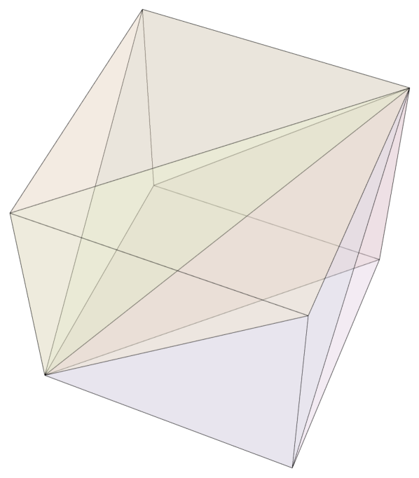
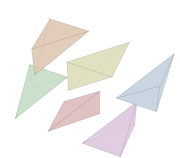
Figure 2: Dissection of $C_{3}$ by the braid hyperplane arrangement, $\mathcal{B}_{3}$, to yield $\mathcal{D}_{\mathcal{B}_{3}}$; an exploded view depicts the individual simplexes more clearly. See Lemma 4.

Fig. 2 also illustrates a property of $\mathcal{D}_{\mathcal{B}_{n}}$ that is crucial to establish ii) in Lemma 4: note that each face is split into two triangles, and each of those triangles is a single-coordinate translation of a triangle on the opposite face. This fact is considered in the proof of Lemma 4 in Section A.1.

Remark 6.

Property ii) of Lemma 4 can also be interpreted as a consequence of the following observation: the braid dissection of a hypercube results in “symmetric” dissections on opposite $n-1$-dimensional faces (c.f. Fig. 2). Thus, dissecting each individual interpolation hypercube this way yields a collection of simplexes that “tile” their union; i.e. a full-dimensional face of any simplex is shared exactly by one and only one other simplex – hence the desired continuity.

Remark 7.

The braid arrangement dissection is a particular dissection by Schäfli orthoschema. [37]

Now we can finally state the proof of Lemma 2.

Proof.

(Lemma 2) The proof will proceed as suggested above. First, we will define the function $\Upsilon_{\omega}$ on the elements of $X_{\eta}$ using the parameter vector $\omega$. Then we will extend $\Upsilon_{\omega}$ to the corners of all the interpolation hypercubes associated with $X_{\eta}$; i.e. we will define $\Upsilon_{\omega}$ on the extra corners of the aforementioned interpolation hypercubes, again in terms of $\omega$ only (see Definition 17). Then we will employ Lemma 3 and Lemma 4 to define a CPWA within each interpolation hypercube that interpolates between the values on its corners – those values being derived exclusively from $\omega$ by the construction above. Finally, Lemma 4 can be used to show that this interpolation scheme is consistent from one interpolation hypercube to the next, thus making it a viable CPWA defined over the entirety of $X$. Moreover, it will also lead to the claimed bound on the number of linear regions needed.

To this end, first define $\Upsilon_{\omega}$ on $X_{\eta}$ as follows. For each $\mathbf{x}_{i}\in X_{\eta}=\{\mathbf{x}_{i}\}_{i=0}^{\scriptscriptstyle|X_{\eta}|-1}$, define: $\Upsilon_{\omega}(\mathbf{x}_{i})\triangleq\pi_{i}(\omega)$. Now, we have to define $\Upsilon_{\omega}$ to the extra corners associated with the interpolation hypercubes of $X_{\eta}$, i.e. $\Delta_{X_{\eta}}$ (see Definition 17). In particular, we extend $\Upsilon_{\omega}$ to $\Delta_{X_{\eta}}$ using the following definition:

$$\forall x\in\Delta_{X_{\eta}}\;.\;\Upsilon_{\omega}(x)\triangleq\min_{\mathbf{x}\in B(x;\eta)\cap X_{\eta}}\Upsilon_{\omega}(\mathbf{x}).$$ (73)

Note that (73) is well defined, since $x\in\Delta_{X_{\eta}}$ is the corner of an interpolation hypercube – which has edge length $\eta$ – and each interpolation hypercube has at least one corner that belongs to $X_{\eta}$; see Fig. 3. Moreover, we have just defined $\Upsilon_{\omega}$ for any such $\mathbf{x}\in X_{\eta}$ in terms of $\omega$ only, so this scheme for defining $\Upsilon_{\omega}$ on $\Delta_{X_{\eta}}$ likewise depends only on $\omega$.

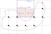
Figure 3: Interpolation Hypercubes. Solid dots denote members of $X_{\eta}$; red dotted lines denote interpolation hypercubes; and $x\in\Delta_{X_{\eta}}$ is an extra corner (see Definition 17).

The previous construction ensures that $\Upsilon_{\omega}$ is defined on the corners of each interpolation hypercube associated with $X_{\eta}$, and thus Lemma 3 and Lemma 4 may be applied to obtain a number of CPWAs, each of whose domains is a single interpolation hypercube. Crucially, however, if these CPWAs are continuous from one interpolation hypercube to any adjacent one, then they may together be considered to define a CPWA whose domain is the union of all such interpolation hypercubes (simply switching between them as appropriate). The result is a CPWA that contains $X$ in its domain. Then, since each individual CPWA requires at most $n!$ linear regions (by Lemma 4), this construction leads to the bound in claim ii) of the Lemma simply by using Proposition 3.

Thus, it remains to show that the CPWAs defined on each interpolation hypercube are consistent (continuous) from one to the next. However, this follows more or less directly from property ii) of Lemma 4. To see this, let $C_{\mathbf{x}\rho}$ be an interpolation hypercube, and let $C_{\mathbf{x}^{\prime}\rho^{\prime}}$ be any other interpolation hypercube that shares an $n-1$-dimensional face, $F_{i}^{k}$, with $C_{\mathbf{x}\rho}$. In particular, both $\Upsilon_{\omega}|_{C_{\mathbf{x}\rho}}$ and $\Upsilon_{\omega}|_{C_{\mathbf{x}^{\prime}\rho^{\prime}}}$ can be regarded as inducing separate functions on the unit hypercube $C_{n}$ (by translation), and because $\Upsilon_{\omega}$ is defined on the corners of all such interpolation hypercubes, these functions satisfy the condition of property ii) of Lemma 4. Thus, their interpolations are identical on opposite faces, which yields the claimed continuity under translation back to domains $C_{\mathbf{x}\rho}$ and $C_{\mathbf{x}^{\prime}\rho^{\prime}}$.∎

4.4 Proof of Theorem 2

Using the consequences of Step 1 (see Section 4.2) and Step 2 (see Section 4.3), we can now prove Theorem 2.

Proof.

By Corollary 2, there is an $\Upsilon_{\omega_{\Psi}}$ that:

• approximates any controller $\Psi$ to the desired accuracy via $\lVert\cdot\rVert_{X}$ merely by changing its parameter values;

• requires no more than the claimed number of linear regions on $X$, given this accuracy, independent of $\Psi$; and

• has a Lipschitz constant at most ${3}\cdot K_{\text{cont}}$ on $X$, also independent of $\Psi$.

By Corollary 1 (a consequence of [2, Theorem 2]) we can find a TLL NN architecture to implement the CPWA $\Upsilon_{\omega_{\Psi}}$. Moreover, if such a TLL is implemented using only linear functions whose Lipschitz constants are bounded by ${3}\cdot K_{\text{cont}}$, as is the case to implement $\Upsilon_{\omega_{\Psi}}$ exactly on $X$, then that TLL will likewise have a global Lipschitz constant of at most ${3}\cdot K_{\text{cont}}$. Thus, Lemma 1 applies, and that completes the proof. ∎

5 Extension: ReLU Architectures for System Identification

The methodology of the previous section can be summarized in the following way: determine the amount of (instantaneous) controller error that can be tolerated relative to a robust controller (Step 1), and design an architecture that can achieve that error for an arbitrary robust controller (Step 2). In particular, though, the methodology of Step 1 – chiefly the Grönwall inequality – only recognizes instantaneous controller error as an error in the (controlled) vector field. As a result, essentially the same calculations can be recycled when the source of error comes not from a different controller, but an alternate, erroneous vector field under the same controller.

Indeed, this is almost a complete program to repurpose the results of Section 4 to obtain assured architectures for system identification. In this context, we treat the instantaneous error as coming from the fact that the identified vector field – a NN in this case – can’t exactly replicate the vector field on which it is trained. Nevertheless, from Step 2, we can find a sufficiently large NN system architecture that can be trained to a proscribed uniform approximation accuracy (relative to the unknown system). This architecture leads to closed-loop assurances under system identification, since a Grönwall calculation – like Proposition 2 of Step 1 – connects training error to a controller robustness margin (and conversely).

In fact, this proposed architecture will lead to something like the following assurance: assuming the architecture has been trained adequately, then an appropriately robust controller designed for the identified system will also control the original, unknown system. In this way, the proposed system identification architecture comes with both a (uniform) training accuracy requirement and a robustness requirement for controllers designed to meet a specification. If these requirements can be met by the identified architecture and a controller designed for said identified architecture, then the very same controller is assured to control the original, unknown system.

This section begins with Section 5.1, in which we formulate an assured NN architecture design problem for system identification. Then, in Section 5.2, we present Theorem 3, which provides just such an assured NN architecture.

5.1 Problem Formulation: NN Architectures for System Identification

As suggested, we will formulate the problem of designing assured architectures for system identification in roughly the reverse way as the controller architecture problem, 2. That is we start from a given accuracy to which the identified dynamics can be learned relative to the original, unknown dynamics; this accuracy will be denoted by the suggestive symbol $\mu>0$. Then the problem will be to find an identified architecture and robustness requirements $\delta$ and $\tau$ such that: if the identified architecture is learned to a uniform error of $\mu$, then any $\delta$-robust controller designed on the identified system will satisfy the same specification on the original system (non-robustly). Hence, we have the following problem of designing assured ReLU architectures for system identification.

Problem 3 (ReLU Architectures for System Identification).

Let $\mu\negthinspace>\negthinspace 0$ and $K_{\text{cont}}\negthinspace>\negthinspace 0$ be given. Let $\Sigma$ be a feedback controllable Lipschitz control system, and let $S_{\text{spec}}\negthinspace=\negthinspace(X_{\text{spec}},U_{\text{spec}},\overset{~{}}{{}_{\scriptscriptstyle S_{\text{spec}}\negthickspace\negthickspace\vphantom{\scriptstyle(}}\negthickspace\negthickspace\negthinspace\longrightarrow})$ be a transition system specification on $\Sigma$.

Then the problem is to find $\tau=\tau(K_{x},K_{u},K_{\text{cont}},\mu)$ and $\delta=\delta(K_{x},K_{u},K_{\text{cont}},\mu)$ together with a ReLU architecture, $\text{Arch}(\Theta)$, which corresponds to an identified system

$$\Sigma^{\Theta}=(X,U,\mathcal{U},{\mathscr{N}\negthickspace\negthickspace\negthinspace\mathscr{N}}\negthinspace_{\Theta}),$$ (74)

where $X$, $U$ and $\mathcal{U}$ are as in $\Sigma$, and ${\mathscr{N}\negthickspace\negthickspace\negthinspace\mathscr{N}}\negthinspace_{\theta}:X\times U\rightarrow X$. The identified system, $\Sigma^{\Theta}$, must further have the properties that:

1. there exists values of $\Theta$ s.t.

   $$\lVert f-{\mathscr{N}\negthickspace\negthickspace\negthinspace\mathscr{N}}\negthinspace_{\Theta}\rVert\leq\mu$$ (75)

   i.e. the architecture is able to learn the vector field $f$ to the proscribed accuracy; and

2. for $\Theta$ as in (75), if $\Psi:X\rightarrow U$ is a $\delta$-$\tau$ invariant Lipschitz-continuous controller with $K_{\Psi}\leq K_{\text{cont}}$ s.t.

   $$S_{\tau}(\Sigma^{\Theta}_{\Psi})\preceq_{\mathcal{AD}_{\delta}}S_{\text{spec}},$$ (76)

   then

   $$S_{\tau}(\Sigma_{\Psi})\preceq_{\mathcal{AD}_{0}}S_{\text{spec}}$$ (77)

   i.e. if $\Psi$ controls the identified system to meet the specification robustly, then $\Psi$ also controls the original system, $S(\Sigma_{\Psi})$, to the same specification (albeit non-robustly).

5.2 ReLU Architectures for Nonlinear-System Identification

Now we have the following theorem, which solves 3 with the claimed guarantees for system identification.

Theorem 3.

Let $\mu>0$ and $K_{\text{cont}}>0$ be given, and let $\Sigma$ and $S_{\text{spec}}$ be as in 3. Furthermore, let $\delta,\tau>0$ be s.t.

$$K_{u}\cdot\mu\cdot\tau\cdot e^{(K_{x}+K_{u}K_{\text{cont}})\tau}<\delta.$$ (78)

If $\eta\leq\tfrac{\mu}{{3}\cdot K_{\text{cont}}}$ is such that there exists an $\eta$-grid of $X\times U$, then an $n$-fold TLL NN architecture $\text{Arch}(\Theta^{\overset{\text{\tiny TLL}\parallel}{~{}}}_{{}^{n+m}_{n}\negthinspace N})$ of size:

$$N\geq(n+m)!\cdot\left\lceil\frac{\text{ext}(X\times U)}{\eta}+2\right\rceil^{n+m}$$ (79)

defines an identified system as in (74) of 3, which has the following properties:

1. there exist values for $\Theta^{\overset{\text{\tiny TLL}\parallel}{~{}}}_{{}^{n+m}_{n}\negthinspace N}$ such that

   $$\lVert f-{\mathscr{N}\negthickspace\negthickspace\negthinspace\mathscr{N}}\negthinspace{\scriptstyle\Theta^{\overset{\text{\tiny TLL}\parallel}{~{}}}_{{}^{n+m}_{n}\negthinspace N}}\rVert_{X\times U}<\mu;\text{ and}$$ (80)

2. for this $\Theta^{\overset{\text{\tiny TLL}\parallel}{~{}}}_{{}^{n+m}_{n}\negthinspace N}$ and $\Psi:X\rightarrow U$ $\delta$-$\tau$ positive invariant w.r.t to $X$ and Lipschitz continuous with $K_{\Psi}\leq K_{\text{cont}}$,

   $$S_{\tau}(\Sigma_{\Psi}\negthinspace\negthinspace\negthinspace{{\scriptstyle\Theta^{\overset{\text{\tiny TLL}\parallel}{~{}}}_{{}^{n+m}_{n}\negthinspace N}}\atop\vphantom{{1\atop 2}}}\negthinspace)\preceq_{\mathcal{AD}_{\delta}}\negthinspace S_{\text{spec}}\negthinspace\negthinspace\implies\negthinspace\negthinspace S_{\tau}(\Sigma_{\Psi}\negthinspace)\preceq_{\mathcal{AD}_{0}}\negthinspace S_{\text{spec}}.$$ (81)

For convenience, denote a trajectory of $\Sigma_{\Psi}\negthinspace\negthinspace\negthinspace{{\scriptstyle\Theta^{\overset{\text{\tiny TLL}\parallel}{~{}}}_{{}^{n+m}_{n}\negthinspace N}}\atop\vphantom{{1\atop 2}}}$ by $\zeta_{x\Psi}^{{\mathscr{N}\negthickspace\negthickspace\negthinspace\mathscr{N}}\negthinspace}$, and
the corresponding vector field by $f^{{\mathscr{N}\negthickspace\negthickspace\negthinspace\mathscr{N}}\negthinspace}$.

Proof.

From the results in Section 4.3, particularly Corollary 2, we know that a parallel TLL architecture of size determined by (79) can indeed approximate the unknown dynamics as required by conclusion i) above. Thus, it remains to show that if this NN is trained to that accuracy with respect to (unknown) $f$, then conclusion ii) holds for a controller, $\Psi$.

To this end, let $\Psi$ be such a controller that is $\delta$-$\tau$ positive invariant, and where $\delta$ and $\tau$ are selected according to the assumptions of the Theorem. Moreover, suppose that $f^{{\mathscr{N}\negthickspace\negthickspace\negthinspace\mathscr{N}}\negthinspace}$ has been trained so that $\lVert f-f^{{\mathscr{N}\negthickspace\negthickspace\negthinspace\mathscr{N}}\negthinspace}\rVert\leq\mu$ for $\mu$ as specified.

Thus, we can proceed as in the proof of Lemma 1. In particular, we seek to bound the difference

$$\lVert\zeta_{x\Psi}(\tau)-\zeta_{x\Psi}^{{\mathscr{N}\negthickspace\negthickspace\negthinspace\mathscr{N}}\negthinspace}(\tau)\rVert<\delta$$ (82)

so that we can construct the appropriate simulation relations. To prove this bound, observe that:

$$\lVert\zeta_{x\Psi}(t)-\zeta_{x\Psi}^{{\mathscr{N}\negthickspace\negthickspace\negthinspace\mathscr{N}}\negthinspace}(t)\rVert$$

$$\negthinspace\negthinspace\leq\negthinspace\negthinspace\negthinspace\int_{0}^{t}\lVert f(\zeta_{x\Psi}(\sigma),\Psi(\zeta_{x\Psi}(\sigma)))-f(\zeta_{x\Psi}^{{\mathscr{N}\negthickspace\negthickspace\negthinspace\mathscr{N}}\negthinspace}(\sigma),\Psi(\zeta_{x\Psi}^{{\mathscr{N}\negthickspace\negthickspace\negthinspace\mathscr{N}}\negthinspace}(\sigma)))\rVert$$

$$\negthinspace+\lVert f(\zeta_{x\Psi}^{{\mathscr{N}\negthickspace\negthickspace\negthinspace\mathscr{N}}\negthinspace}(\sigma),\Psi(\zeta_{x\Psi}^{{\mathscr{N}\negthickspace\negthickspace\negthinspace\mathscr{N}}\negthinspace}(\sigma)))-f^{{\mathscr{N}\negthickspace\negthickspace\negthinspace\mathscr{N}}\negthinspace}(\zeta_{x\Psi}^{{\mathscr{N}\negthickspace\negthickspace\negthinspace\mathscr{N}}\negthinspace}(\sigma),\Psi(\zeta_{x\Psi}^{{\mathscr{N}\negthickspace\negthickspace\negthinspace\mathscr{N}}\negthinspace}(\sigma)))\rVert d\sigma$$

$$\negthinspace\negthinspace\leq\negthinspace\negthinspace\negthinspace\negthinspace\int_{0}^{t}(K_{x}+K_{u}K_{\text{cont}})\cdot\lVert\zeta_{x\Psi}(\sigma)-\zeta_{x\Psi}^{{\mathscr{N}\negthickspace\negthickspace\negthinspace\mathscr{N}}\negthinspace}(\sigma)\rVert+\lVert f-f^{{\mathscr{N}\negthickspace\negthickspace\negthinspace\mathscr{N}}\negthinspace}\rVert_{\scriptscriptstyle X\times U}d\sigma$$ (83)

where the last inequality follows from the fact that $\Psi$ was assumed to be designed such that it is $\delta$-$\tau$ positive invariant with respect to $X$ (and by construction $\Psi$ has codomain $U$). Of course the Grönwall inequality applies to (83) when we use the assumed training error bound $\lVert f-f^{{\mathscr{N}\negthickspace\negthickspace\negthinspace\mathscr{N}}\negthinspace}\rVert\leq\mu$. Since $\delta$ and $\tau$ were chosen according to (78) – which has exactly the form of the Grönwall bound obtained in (83) – we conclude that (82) holds. Hence, the conclusion of the Theorem follows by way of arguments already discussed in Section 4. ∎

6 Conclusion

In this paper, we considered the problem of automatically designing assured ReLU NN architectures for both control and system identification of nonlinear control systems. To the best of our knowledge, our approach uniquely leverages the flexible TLL architecture and a generic specification paradigm via ADS in order to do automatic, assured NN architecture design for incompletely known nonlinear systems. We thus expect this work to serve as a starting point for further work on the problem of automatic NN architecture design, particularly with closed-loop dynamical specifications in mind. In conclusion, we offer two observations that present opportunities for generalization.

First, we note that in this paper, we have constructed CPWA functions in terms of their linear regions (see Step 2 of the proof of Theorem 2: Section 4.3). This construction by linear regions is ideally suited for conversion to TLL NNs using Theorem 1. However, in this paper, we have obtained these linear regions by a specific construction: first by setting down a regular grid of interpolation hypercubes and then subdividing those hypercubes into simplexes using the braid hyperplane arrangement. This scheme works because grid of hypercubes controls the size of the resulting simplexes, and the braid arrangement ensures that any full-dimensional face of one simplex is exactly shared by one and only one other simplex – i.e. it constitutes a “tiling”, which leads to a continuous piecewise function. However, this specific construction is not needed to employ Theorem 1 to obtain a TLL network: any other “tiling” by sufficiently small simplexes could be converted to a TLL approximate controller just as easily. Thus, a direction of future work would be to find a more efficient (or even minimal) “tiling” by simplexes, which would lead to smaller architectures.

Second, we make a similar observation but in the other direction. In particular, we have chosen to convert the above-described approximate CPWA controller specifically to a TLL NN, but a TLL may not be the most neuron-efficient NN representation. In other words, there may be other architectures that can represent the same, approximate CPWA controller using considerably fewer neurons. Thus, another compelling direction of future research would be to seek more compact assured architectures by exploring classes of NN architectures other than TLL NNs.

7 Acknowledgments

The authors wish to thank Xiaowu Sun (University of California, Irvine) for noting by example that a function defined on the corners of a hypercube can be extended by a CPWA that uses fewer regions than in Lemma 4 of [3].

Appendix A Appendix

A.1 Proof of Lemma 4

To prove Lemma 4, we need a few preliminary results.

Proposition 4 (Coordinate Orderings and Braid Arrangements Regions [36]).

Let $\mathcal{B}_{n}$ be the braid arrangement defined in Lemma 4. Then for each (open) region $R$ of $\mathcal{B}_{n}$ there is a unique permutation $\sigma_{R}:\{1,\dots,n\}\rightarrow\{1,\dots,n\}$ such that

$$\forall x\in R\;.\;\sigma_{R}(i)<\sigma_{R}(j)\implies\pi_{\sigma_{R}(i)}(x)<\pi_{\sigma_{R}(j)}(x).$$ (84)

In other words, the coordinates of any point in $R$ can be sorted into ascending order using a single, common permutation, and this permutation is unique to $R$.

Proof.

See [36]. ∎

Lemma 5.

Let $\mathcal{B}_{n}$ be the braid arrangement, and let $\mathcal{D}_{\mathcal{B}_{n}}$ be the braid dissection of $C_{n}$ (both as defined in Lemma 4).

Then any region $R$ of $\mathcal{B}_{n}$ intersects exactly one $n-1$-dimensional face not containing the origin, i.e.

$$\mathsf{F}_{i}^{R}\triangleq R\cap F_{i}^{1}$$ (85)

is nonempty for exactly one $i=i_{R}\in\{1,\dots,n\}$. Moreover, for any two distinct regions $R$ and $R^{\prime}$ of $\mathcal{B}_{n}$,

$$\mathsf{F}_{R}\cap\mathsf{F}_{{R^{\prime}}}=\emptyset,$$ (86)

where the notation $\mathsf{F}_{i_{R}}^{R}$ is simplified to $\mathsf{F}_{R}$ by the above claim.

Finally, for each $R$, the closure $\overline{\mathsf{F}_{R}}$ is isomorphic to a region $P$ of the braid dissection $\mathcal{D}_{\mathcal{B}_{n-1}}$ by means of the projection and embedding ($e_{i}$ is a column of the $(n\times n)$ identity matrix):

$$\pi_{\neg i} :\mathbb{R}^{\scriptscriptstyle n}\rightarrow\mathbb{R}^{\scriptscriptstyle n-1},\;\pi_{\neg i}:x\mapsto\left(\begin{smallmatrix}e_{1}&\dots&e_{i-1}&e_{i+1}&\dots e_{n}\end{smallmatrix}\right)^{\scriptscriptstyle\text{T}}x$$ (87)

$$\mathscr{I}_{i}^{k} :\mathbb{R}^{\scriptscriptstyle n-1}\rightarrow\mathbb{R}^{\scriptscriptstyle n},\;\mathscr{I}_{i}^{k}:x\mapsto(\begin{smallmatrix}e_{1}&\dots&e_{i-1}&e_{i+1}&\dots e_{n}\end{smallmatrix})x+k\cdot e_{i}$$ (88)

i.e. $\pi_{\neg i}:\mathsf{F}_{R}\rightarrow P$ is a bijection that maps corners of $C_{n}$ to corners of $C_{n-1}$; its inverse is $\mathscr{I}_{i}^{1}:P\rightarrow\mathsf{F}_{R}$.

Proof.

First, we claim that the any region $R$ of $\mathcal{B}_{n}$ intersects the exactly one $F_{i}^{1}$. This follows because each point in (the open set) $R$ necessarily has the same unique maximal coordinate by Proposition 4; identify this maximal coordinate as $i_{R}$. Hence, $R$ intersects $F_{i_{R}}^{1}$, since every element $x\in\text{int}(F_{i}^{1})$ likewise has the same unique maximal coordinate of $\pi_{i}(x)=1$. Indeed, consider the point

$$x^{\prime}=(\tfrac{\sigma_{R}(1)}{\sigma_{R}(1)+1}\hskip 0.85358pt\dots\hskip 0.85358pt\tfrac{\sigma_{R}(i_{R}-1)}{\sigma_{R}(i_{R}-1)+1}\hskip 1.42262pt\;1\;\hskip 1.42262pt\tfrac{\sigma_{R}(i_{R}+1)}{\sigma_{R}(i_{R}+1)+1}\hskip 0.85358pt\dots\hskip 0.85358pt\tfrac{\sigma_{R}(n)}{\sigma_{R}(n)+1})$$ (89)

which lies in: $F_{i_{R}}^{1}$ because of its $i_{R}^{\text{th}}$ coordinate; and in $R$ because its coordinates respect the sorting associated with $R$. To show the second claim, merely note that the regions of $\mathcal{B}_{n}$ are disjoint by definition (they are regions of a hyperplane arrangement), so $R\neq R^{\prime}$ implies that $F_{R}\cap F_{R^{\prime}}=\emptyset$.

Finally, consider $\overline{\mathsf{F}_{R}}$ for $R$ in $\mathcal{B}_{n}$. We claim $\overline{\mathsf{F}_{R}}$ is isomorphic to the region in $\mathcal{D}_{\mathcal{B}_{n-1}}$ given by $P=\overline{R^{\prime}\cap\text{int}(C_{n-1})}$, where $R^{\prime}$ is the region of $\mathcal{B}_{n-1}$ associated with:

$$\sigma_{R^{\prime}}:i\mapsto\begin{cases}\sigma_{R}(i)&i<i_{R}\\ \sigma_{R}(i+1)&i\geq i_{R}\end{cases}$$ (90)

which is in effect the ordering $\sigma_{R}$ with its maximal element excluded. Thus, any point $x\in R$ maps to a point in $P$ so defined, since it trivially maps to a point in $R^{\prime}$ via $\pi_{\neg i}$. Likewise, any point in $P\cap R^{\prime}$ maps to a point in $R\cap F_{i_{R}}^{1}$ by the inclusion of the additional coordinate specified by $\mathscr{I}_{i_{R}}^{1}$. Furthermore, these mappings extend to the closed sets specified by continuity. It follows that corners of one set are mapped to corners of the other and vice versa, since $\pi_{\neg i}$ and $\mathscr{I}_{i_{R}}^{1}$ either remove or include a coordinate with value 1. ∎

Now we can state formally state the proof of Lemma 4.

Proof.

We claim that the dissection $\mathcal{D}_{\mathcal{B}}$ (see (71)) consists of exactly $n!$ simplexes, each of whose vertices are in $\mathcal{F}_{0}(C)$. Thus, $\Xi_{\alpha}^{\mathcal{B}_{n}}$ has at most $n!$ linear regions, one for each simplex.

First, note that the interior of each region of $\mathcal{B}$ intersects $\text{int}(C_{n})$; this is because all possible coordinate orderings of the point $(\tfrac{1}{2},\tfrac{1}{3},\dots,\tfrac{1}{n+1})$ are contained in $\text{int}(C_{n})$. Hence, each region of $\mathcal{B}_{n}$ contributes one region to $\mathcal{D}_{\mathcal{B}_{n}}$, so $|\mathcal{D}_{\mathcal{B}_{n}}|=n!$.

Thus, it remains to show that the intersection of $C_{n}$ with each region in $\mathcal{B}$ is in fact an $n$-simplex, and we show this by induction on dimension. As the base case, consider $n=2$. In particular, $\mathcal{B}_{2}$ has only one hyperplane, and it dissects $C_{2}$ into two triangles (i.e. $2$-simplexes), each of whose vertices are vertices of the square $C_{2}$. Hence, suppose that $\mathcal{B}_{n}$ divides $C_{n}$ into $n$-simplexes with vertices from $\mathscr{F}_{0}(C_{n})$; we will show that this implies that $\mathcal{B}_{n+1}$ divides $C_{n+1}$ into $n+1$-simplexes, each of whose vertices are from $\mathscr{F}_{0}(C_{n+1})$.

To complete the proof of the induction step, let $R$ be a region from $\mathcal{B}_{n+1}$, and observe that for any $x\in R\cap\text{int}(C_{n+1})$ and any $t>0$, $t\cdot x$ remains in $R$, since multiplication by a non-negative scalar doesn’t change the ordering of the coordinates of $x$. For a similar reason, there is a $t_{\text{max}}(x)\in\mathbb{R}$ such that

$$t_{\text{max}}(x)\triangleq\sup_{t\cdot x\in C_{n+1}}t=\sup_{t\cdot\max_{i}\pi_{i}(x)<1}t.$$ (91)

Thus, we conclude that $R\cap\text{int}(C_{n+1})$ is the interior of a cone that extends from the origin, and it has a (convex) base contained entirely in some $F_{i_{R}}^{1}$ by Lemma 5; indeed, that base is isomorphic to $\overline{C_{n}\cap R^{\prime}}$ where $R^{\prime}$ is a region from $\mathcal{B}_{n}$. Of course, by the induction hypothesis, $\overline{C_{n}\cap R^{\prime}}$ is an $n$-simplex whose vertices are contained in $\mathscr{F}_{0}(C_{n})$, so the base of the cone $\overline{R\cap C_{n+1}}$ is necessarily an $n$-simplex whose vertices lie in $F_{i_{R}}^{k}\cap\mathscr{F}_{0}(C_{n+1})$, again by Lemma 5. Thus, those vertices, together with the origin, constitute the $n+2$ vertices of $\overline{R\cap\text{int}(C_{n+1})}$, and each vertex is a corner of $C_{n+1}$ by construction. Hence, $\overline{R\cap\text{int}(C_{n+1})}$ is an $n+1$ simplex whose vertices are in $\mathscr{F}_{0}(C_{n+1})$ as claimed.

It remains to show that this $\Xi_{\alpha}^{\mathcal{B}_{n}}$ satisfies ii). To wit, let $\alpha,\alpha^{\prime}\negthinspace:\negthinspace\mathscr{F}_{0}(C)\negthinspace\rightarrow\negthinspace\mathbb{R}$, and assume without loss of generality that $k=1$ so that

$$\forall x\in F_{i}^{1}\cap\mathscr{F}_{0}(C)\;.\;\alpha(x)=\alpha^{\prime}(|x-e_{i}|).$$ (92)

Now let $R$ be a region of $\mathcal{B}_{n}$ with $R\cap F_{i_{R}}^{1}\neq\emptyset$. It suffices to show that there is a region $R^{\prime}$ with $R^{\prime}\cap\text{int}(F_{i}^{0})\neq\emptyset$ such that $\overline{R\cap F_{i}^{1}}$ and $\overline{R^{\prime}\cap F_{i}^{0}}$ are isomorphic under the (self-inverse) translation map $\mathcal{T}_{i}:x\mapsto|x-e_{i}|$. This is because $\Xi_{\alpha}^{\mathcal{B}_{n}}$ and $\Xi_{\alpha^{\prime}}$ linearly interpolate between the values of $\alpha$ and $\alpha^{\prime}$ on $\overline{R\cap F_{i}^{1}}$ and $\overline{R^{\prime}\cap F_{i}^{0}}$, respectively, and $\alpha$ and $\alpha^{\prime}$ agree on translates of these points in their domains. For example, consider the illustration of $\mathcal{D}_{\mathcal{B}_{3}}$ shown in Fig. 2: note that any triangle (2-simplex) created by $\mathcal{D}_{\mathcal{B}_{3}}$ on one face is the single-coordinate translate of a triangle created by $\mathcal{D}_{\mathcal{B}_{3}}$ on the opposite face.

However, this follows as a more or less direct consequence of Lemma 5. Indeed, we note that $\overline{R\cap F_{i_{R}}^{1}}$ is isomorphic to some $P\in\mathcal{D}_{\mathcal{B}_{n-1}}$ derived from a region $R^{\prime}_{n-1}$ in $\mathcal{B}_{n-1}$. But it is easy to see that this $P$ is isomorphic to a set of the claimed form $\overline{R^{\prime}\cap F_{i_{R}}^{0}}$, by using the inclusion map $\mathscr{I}_{i_{R}}^{0}$ instead of $\mathscr{I}_{i_{R}}^{1}$ – and with the usual inverse $\pi_{\neg i_{R}}$ (see Lemma 5). ∎

[]James Ferlez received a B.S. and M.S. in Electrical Engineering from the Pennsylvania State University, University Park, PA in 2008 and 2009, respectively, and earned a PhD in Electrical Engineering from the University of Maryland, College Park in 2019.

He is currently a Postdoctoral Researcher at the University of California, Irvine in the Resilient Cyber-Physical Systems Laboratory. His research interests include formal methods for control, neural networks, machine learning and stochastic control.

[]Yasser Shoukry (Member, IEEE) is an Assistant Professor in the Department of Electrical Engineering and Computer Science at the University of California, Irvine. He received his Ph.D. in Electrical Engineering from the University of California, Los Angeles in 2015. He received the M.Sc. and the B.Sc. degrees (with distinction and honors) in Computer and Systems engineering from Ain Shams University, Cairo, Egypt in 2010 and 2007, respectively. Between September 2015 and July 2017, Yasser was a joint post-doctoral associate at UC Berkeley, UCLA, and UPenn. Before pursuing his Ph.D. at UCLA, he spent four years as an R&D engineer in the industry of automotive embedded systems. Yasser’s research interests include the design and implementation of resilient Cyber–Physical Systems (CPS) and Internet-of-Things (IoT) by drawing on tools from embedded systems, formal methods, control theory, and machine learning.

Prof. Shoukry is the recipient of the IEEE TC-CPS Early Career Award in 2021, the NSF CAREER award in 2019, the Best Demo Award from the ACM/IEEE IPSN conference in 2017, the Best Paper Award from the ACM/IEEE ICCPS in 2016 and the Distinguished Dissertation Award from UCLA EE department in 2016. In 2015, he led the UCLA/Caltech/CMU team to win the NSF Early Career Investigators (NSF-ECI) research challenge. His team represented the NSF-ECI in the NIST Global Cities Technology Challenge, an initiative designed to advance the deployment of Internet of Things (IoT) technologies within a smart city. He is also the recipient of the 2019 George Corcoran Memorial Award for his contributions to teaching and educational leadership in the field of CPS and IoT.

References

- [1] M. Bojarski, D. Del Testa, D. Dworakowski, B. Firner, B. Flepp, P. Goyal, L. D. Jackel, M. Monfort, U. Muller, J. Zhang, et al., “End to end learning for self-driving cars,” arXiv:1604.07316, 2016.
- [2] J. Ferlez and Y. Shoukry, “AReN: Assured ReLU NN Architecture for Model Predictive Control of LTI Systems,” in Hybrid Systems: Computation and Control 2020 (HSCC’20), ACM, New York, 2020.
- [3] J. Ferlez, X. Sun, and Y. Shoukry, “Two-Level Lattice Neural Network Architectures for Control of Nonlinear Systems,” in 2020 59th IEEE Conference on Decision and Control (CDC), pp. 2198–2203, 2020.
- [4] T. Elsken, J. H. Metzen, and F. Hutter, “Neural Architecture Search: A Survey,” Journal of Machine Learning Research, vol. 20, no. 55, pp. 1–21, 2019.
- [5] H. Mendoza, A. Klein, M. Feurer, J. T. Springenberg, and F. Hutter, “Towards Automatically-Tuned Neural Networks,” in Workshop on Automatic Machine Learning, pp. 58–65, PMLR, 2016.
- [6] B. Baker, O. Gupta, R. Raskar, and N. Naik, “Accelerating Neural Architecture Search using Performance Prediction,” in Workshop on Meta-Learning (MetaLearn), p. 7, 2017.
- [7] H. Cai, T. Chen, W. Zhang, Y. Yu, and J. Wang, “Efficient Architecture Search by Network Transformation,” 2017.
- [8] B. Zoph, V. Vasudevan, J. Shlens, and Q. V. Le, “Learning Transferable Architectures for Scalable Image Recognition,” in 2018 IEEE/CVF Conference on Computer Vision and Pattern Recognition, pp. 8697–8710, IEEE, 2018.
- [9] B. Baker, O. Gupta, N. Naik, and R. Raskar, “Designing neural network architectures using reinforcement learning,” arXiv:1611.02167, 2016.
- [10] B. Zoph and Q. Le, “Neural Architecture Search with Reinforcement Learning,” in International Conference on Learning Representations (ICLR), 2017.
- [11] J. Bergstra and Y. Bengio, “Random search for hyper-parameter optimization,” Journal of Machine Learning Research, vol. 13, no. Feb, pp. 281–305, 2012.
- [12] T. Elsken, J. H. Metzen, and F. Hutter, “Efficient Multi-Objective Neural Architecture Search via Lamarckian Evolution,” 2018.
- [13] E. Real, A. Aggarwal, Y. Huang, and Q. V. Le, “Regularized Evolution for Image Classifier Architecture Search,” Proceedings of the AAAI Conference on Artificial Intelligence, vol. 33, no. 01, pp. 4780–4789, 2019.
- [14] S. Xie, H. Zheng, C. Liu, and L. Lin, “SNAS: Stochastic neural architecture search,” 2018.
- [15] Y. Zhang, S. Chen, C. Diao, and B. Xian, “A direct NN-approximation control for uncertain nonaffine systems with unknown control direction,” International Journal of Robust and Nonlinear Control, vol. 30, no. 3, pp. 864–881, 2020.
- [16] C. Wang, M. Wang, T. Liu, and D. J. Hill, “Learning From ISS-Modular Adaptive NN Control of Nonlinear Strict-Feedback Systems,” IEEE Transactions on Neural Networks and Learning Systems, vol. 23, no. 10, pp. 1539–1550, 2012.
- [17] S. Ge and C. Wang, “Direct adaptive NN control of a class of nonlinear systems,” IEEE Transactions on Neural Networks, vol. 13, no. 1, pp. 214–221, 2002.
- [18] T. Hayakawa, W. M. Haddad, and K. Y. Volyanskyy, “Neural network hybrid adaptive control for nonlinear uncertain impulsive dynamical systems,” Nonlinear Analysis: Hybrid Systems, vol. 2, no. 3, pp. 862–874, 2008.
- [19] A. Aydinoglu, M. Fazlyab, M. Morari, and M. Posa, “Stability analysis of complementarity systems with neural network controllers,” in Proceedings of the 24th International Conference on Hybrid Systems: Computation and Control, no. 19, pp. 1–10, Association for Computing Machinery, 2021.
- [20] Q. Zhao, X. Chen, Y. Zhang, M. Sha, Z. Yang, W. Lin, E. Tang, Q. Chen, and X. Li, “Synthesizing ReLU neural networks with two hidden layers as barrier certificates for hybrid systems,” in Proceedings of the 24th International Conference on Hybrid Systems: Computation and Control, no. 17, pp. 1–11, Association for Computing Machinery, 2021.
- [21] Y.-S. Wang, L. Weng, and L. Daniel, “Neural Network Control Policy Verification With Persistent Adversarial Perturbation,” in International Conference on Machine Learning, pp. 10050–10059, PMLR, 2020.
- [22] S. S. Pon Kumar, A. Tulsyan, B. Gopaluni, and P. Loewen, “A Deep Learning Architecture for Predictive Control,” IFAC-PapersOnLine, vol. 51, no. 18, pp. 512–517, 2018.
- [23] Y. Chen, Y. Shi, and B. Zhang, “Optimal Control Via Neural Networks: A Convex Approach,” 2018.
- [24] S. CHEN, S. A. BILLINGS, and P. M. GRANT, “Non-linear system identification using neural networks,” International Journal of Control, vol. 51, no. 6, pp. 1191–1214, 1990.
- [25] O. Ogunmolu, X. Gu, S. Jiang, and N. Gans, “Nonlinear Systems Identification Using Deep Dynamic Neural Networks,” 2016.
- [26] M. Fält and P. Giselsson, “System Identification for Hybrid Systems using Neural Networks,” 2019.
- [27] J. Velázquez-Velázquez, R. Galván-Guerra, and I. Baruch, “Hybrid Recurrent Neural Network for Nonlinear Hybrid Dynamical Systems Identification,” in 2011 8th International Conference on Electrical Engineering, Computing Science and Automatic Control, pp. 1–6, 2011.
- [28] W. Sun and T. Winn, “A General Lattice Representation for Explicit Model Predictive Control,” 2011.
- [29] J. He, L. Li, J. Xu, and C. Zheng, “ReLU deep neural networks and linear finite elements,” Journal of Computational Mathematics, vol. 38, no. 3, pp. 502–527, 2020.
- [30] H. K. Khalil, Nonlinear Systems. Pearson, Third ed., 2001.
- [31] M. Zamani, G. Pola, M. Mazo, and P. Tabuada, “Symbolic Models for Nonlinear Control Systems Without Stability Assumptions,” IEEE Transactions on Automatic Control, vol. 57, no. 7, 2012.
- [32] P. Tabuada, Verification and Control of Hybrid Systems: A Symbolic Approach. Springer US, 2009.
- [33] V. Kurtz, P. M. Wensing, and H. Lin, “Robust Approximate Simulation for Hierarchical Control of Linear Systems under Disturbances,” 2020.
- [34] K. Mallik, A.-K. Schmuck, S. Soudjani, and R. Majumdar, “Compositional Synthesis of Finite-State Abstractions,” IEEE Transactions on Automatic Control, vol. 64, no. 6, pp. 2629–2636, 2019.
- [35] G. Pola, A. Girard, and P. Tabuada, “Approximately bisimilar symbolic models for nonlinear control systems,” Automatica, vol. 44, no. 10, pp. 2508–2516, 2008.
- [36] R. P. Stanley, “An Introduction to Hyperplane Arrangements,” p. 90.
- [37] H. S. M. Coxeter, Regular Polytopes. Courier Corporation, 1973.