A Multivariate Spline based Collocation Method for
Numerical Solution of Partial Differential Equations

Abstract

We propose a collocation method based on multivariate polynomial splines over triangulation or tetrahedralization for numerical solution of partial differential equations. We start with a detailed explanation of the method for the Poisson equation and then extend the study to the second order elliptic PDE in non-divergence form. We shall establish the convergence of our method and show that the numerical solution can approximate the exact PDE solution very well. Then we present a large amount of numerical experimental results to demonstrate the performance of the method over the 2D and 3D settings. In addition, we present a comparison with the existing multivariate spline methods in [2] and [12] to show that the new method produces a similar and sometimes more accurate approximation in a more efficient fashion.

1 Introduction

In this paper, we propose and study a new collocation method based on multivariate splines for numerical solution of partial differential equations over polygonal domain in $\mathbb{R}^{d}$ for $d\geq 2$. Instead of using a second order elliptic equation in divergence form:

$$\left\{\begin{array}[]{cl}-\sum_{i,j=1}^{d}\frac{\partial}{\partial x_{i}}(a^{ij}(x)\frac{\partial}{\partial x_{j}}u)+\sum_{i=1}^{d}b^{i}(x)\frac{\partial}{\partial x_{i}}u+c^{1}(x)u&=f,\quad x\in\Omega\subset\mathbb{R}^{d},\cr u&=g,\quad\hbox{ on }\partial\Omega\end{array}\right.$$ (1)

which is often used for various finite element methods, we discuss in this paper a more general form of second order elliptic PDE in non-divergence form:

$$\left\{\begin{array}[]{cl}\sum_{i,j=1}^{d}a^{ij}(x)\frac{\partial}{\partial x_{i}}\frac{\partial}{\partial x_{j}}u+\sum_{i=1}^{d}b^{i}(x)\frac{\partial}{\partial x_{i}}u+c(x)u&=f,\quad x\in\Omega\subset\mathbb{R}^{d},\cr u&=g,\quad\hbox{ on }\partial\Omega,\end{array}\right.$$ (2)

where the PDE coefficient functions $a^{ij}(x),i,j=1,\cdots,d$ are in $L^{\infty}(\Omega)$ and satisfy the standard elliptic condition. In addition, when $d\geq 2$, we shall assume the so-called Cordés condition, see (28) in a later section or see [19].

Numerical solutions to the 2nd order PDE in the non-divergence form have been studied extensively recently. See some studies in [19], [12], [16], [20], [18], and etc.. The method in this paper provides a new and more effective approach. In this paper, we mainly use the Sobolev space $H^{2}(\Omega)$. It is known when $\Omega$ is convex (cf. [6]), the solution to the Poisson equation with zero boundary condition, i.e. $g=0$ will be in $H^{2}(\Omega)$. Recently, the researchers in [5] showed that when $\Omega$ has an uniformly positive reach, the solution of (2) with zero boundary condition will be in $H^{2}(\Omega)$. Various domains of uniformly positive reach, e.g. star-shaped domain and domains with holes are shown in [5]. See more examples in the next preliminary section. Many more domains other than convex domains can have $H^{2}$ solution. For any $u\in H^{2}(\Omega)$, we use the standard $H^{2}$ norm

$$\|u\|_{H^{2}}=\|u\|_{L^{2}(\Omega)}+\|\nabla u\|_{L^{2}(\Omega)}+\sum_{i,j=1}^{d}\|\frac{\partial}{\partial x_{i}}\frac{\partial}{\partial x_{j}}u\|_{L^{2}(\Omega)}$$ (3)

for all $u$ on $H^{2}(\Omega)$ and the semi-norm

$$|u|_{H^{2}}=\sum_{i,j=1}^{d}\|\frac{\partial}{\partial x_{i}}\frac{\partial}{\partial x_{j}}u\|_{L^{2}(\Omega)}.$$ (4)

Since we will use multivariate spline functions to approximate the solution $u\in H^{2}(\Omega)$, we use $C^{r}$ smooth spline functions with $r\geq 1$ and the degree $D$ of splines sufficiently large satisfying $D\geq 3r+2$ in $\mathbb{R}^{2}$ and $D\geq 6r+3$ in $\mathbb{R}^{3}$. Let $S^{r}_{D}(\triangle)$ be the spline space of degree $D$ and smoothness $r$ over triangulation or tetrahedralization $\triangle$ of $\Omega$. How to use such spline functions has been explained in [14], [2], [17], and [18], and etc.. For convenience, we shall give a preliminary on multivariate splines in the next section.

We now explain our spline based collocation method. For simplicity, we use the standard Poisson equation which is a special case of the PDE (2).

$$\left\{\begin{array}[]{cl}-\Delta u&=f,\quad{\hbox{ in }}\Omega\subset\mathbb{R}^{d},\cr u&=g,\quad\hbox{ on }\partial\Omega.\end{array}\right.$$ (5)

When $\Omega$ has a uniform positive reach, the solution to the Poisson equation will be in $H^{2}(\Omega)$. We shall use $C^{r}$ spline functions with $r\geq 2$ to approximate the solution $u$. In addition, we shall use the so-called domain points (cf. [10] or the next section) to be the collocation points. Letting $\xi_{i},i=1,\cdots,N$ be the domain points of $\triangle$ and degree $D^{\prime}>0$, where $D^{\prime}$ will be different from $D$, our multivariate spline based collocation method is to seek a spline function $s\in S^{r}_{D}(\triangle)$ satisfying

$$\left\{\begin{array}[]{cl}-\Delta s(\xi_{i})&=f(\xi_{i}),\quad\forall\xi_{i}\in\Omega\subset\mathbb{R}^{d},\cr s(\xi_{i})&=g(\xi_{i}),\quad\forall\xi_{i}\in\partial\Omega,\end{array}\right.$$ (6)

where $i=1,\cdots,N$. It is known a multivariate spline space is a linear vector space which is spanned by a set of basis functions. However, it is difficult to construct locally supported basis functions in $C^{r}(\Omega)$ with $r\geq 1$ due to the complication of the smoothness conditions over $\triangle$. Typically, any small perturbation of a vertex in $\triangle$ may change the dimension of $S^{r}_{D}(\triangle)$. On the other hand, the smoothness conditions can be written as a system of linear equations, i.e. $H{{\bf c}}=0$, where ${\bf c}$ is the coefficient vector of spline function $s\in S^{r}_{D}(\triangle)$ and $H$ is the matrix consisting of all smoothness condition across each interior edge of $\triangle$ (cf. [10] or the next section). To overcome this difficulty of constructing locally supported basis spline functions, we will begin with a discontinuous spline space $s\in S^{-1}_{D}(\triangle)$ and then add the smoothness conditions $H{\bf c}=0$ as constraints in addition to the constraint of boundary condition. One of the key ideas is to let a computer decide how to choose ${\bf c}$ to satisfy $H{\bf c}=0$ and (6) above simultaneously. Clearly, (6) leads to a linear system which may not have a unique solution. It may be an over-determined linear system if $D^{\prime}>D$ or an under-determined linear system if $D^{\prime}<D$. Our method is to use a least squares solution if the system is overdetermined or a sparse solution if the system is under-determined (cf. [13]).

To establish the convergence of the spline based collocation solution as the size of $\triangle$ goes to zero, we define a new norm $\|u\|_{L}$ on $H^{2}(\Omega)\cap H^{1}_{0}(\Omega)$ for the Poisson equation as follows.

$$\|u\|_{L}=\|\Delta u\|_{L^{2}(\Omega)}.$$ (7)

We will show that the new norm is equivalent to the standard norm on Banach space $H^{2}(\Omega)\cap H^{1}_{0}(\Omega)$. That is,

Theorem 1

Suppose $\Omega\subset\mathbb{R}^{d}$ be a bounded domain and the closure of $\Omega$ is of uniformly positive reach $r_{\Omega}>0$. Then there exist two positive constants $A$ and $B$ such that

$$A\|u\|_{H^{2}}\leq\|u\|_{L}\leq B\|u\|_{H^{2}},\quad\forall u\in H^{2}(\Omega)\cap H^{1}_{0}(\Omega).$$ (8)

See the proof of Theorem 4 in a later section. Letting $u\in H^{2}(\Omega)\cap H^{1}_{0}(\Omega)$ be the solution of (5) with $g=0$ and $u_{s}$ be the spline solution of (6), we use the first inequality above to have

$$A\|u-u_{s}\|_{H^{2}}\leq\|u-u_{s}\|_{L}.$$

It can be seen from (6) that the first equation can be written as

$$\Delta(u_{s}(\xi_{i})-u(\xi_{i}))=0,i=1,\cdots,N$$ (9)

which is a discretization of $\|u-u_{s}\|_{L}^{2}$. Let $|\triangle|$ be the size of triangulation or tetrahedralization $\triangle$. Since we can use a spline function to approximate $u$ if $u$ is sufficiently smooth when the size $|\triangle|$ goes to zero (cf. [10]), we seek the minimizer $u_{s}$ of a minimization to be explained in a later section. Then the root mean square error (RMSE) will be small for a sufficiently large amount of collocation points and distributed evenly when the size $|\triangle|$ of $\triangle$ is small. Then our Theorem 1 implies that $\|u-u_{s}\|_{H^{2}}$ is small. Furthermore, we will show

$$\|u-u_{s}\|_{L^{2}(\Omega)}\leq C|\triangle|^{2}\|u-u_{s}\|_{L}\hbox{ and }\|\nabla(u-u_{s})\|_{L^{2}(\Omega)}\leq C|\triangle|\|u-u_{s}\|_{L}$$ (10)

for a positive constant $C$, under the assumption that $u-u_{s}=0$ on $\partial\Omega$. These will establish the multivariate spline based collocation method for the Poisson equation.

In general, we let ${\cal L}$ be the PDE operator in (11). Note that we begin with the second order term of the PDE just for convenience.

$$\left\{\begin{array}[]{cl}\displaystyle\sum_{i,j=1}^{d}a^{ij}(x)\frac{\partial}{\partial x_{i}}\frac{\partial}{\partial x_{j}}u&=f,\quad x\in\Omega\subset\mathbb{R}^{d},\cr u&=g,\quad\hbox{ on }\partial\Omega,\end{array}\right.$$ (11)

We shall similarly define a new norm associated with the PDE (11):

$$\|u\|_{\cal L}=\|{\cal L}(u)\|_{L^{2}(\Omega)}.$$ (12)

Similarly we will show the following.

Theorem 2

Suppose $\Omega\subset\mathbb{R}^{d}$ be a bounded domain and the closure of $\Omega$ is of uniformly positive reach $r_{\Omega}>0$. Suppose that the second order partial differential equation in (11) is elliptic, i.e. satisfying (27) and satisfies the Cordés condition if $d\geq 2$. There exist two positive constants $A_{1}$ and $B_{1}$ such that

$$A_{1}\|u\|_{H^{2}}\leq\|u\|_{\cal L}\leq B_{1}\|u\|_{H^{2}},\quad\forall u\in H^{2}(\Omega)\cap H^{1}_{0}(\Omega).$$ (13)

See a proof in a section later. Similar to the Poisson equation setting, this result will enable us to establish the convergence of the spline based collocation method for the second order elliptic PDE in non-divergence form. Also, we will have the improved convergence similar to (10).

In addition to the major advantages of spline functions: the flexibility of the degree, the tailorable smoothness of splines, the property of partition of the unity of Bernstein-Bézier polynomials, there are a few more advantages of the spline based collocation methods over the traditional finite element methods, discontinuous Galerkin methods, virtual element methods, and etc.. For example, no weak formulation of the PDE solution is required and hence, no numerical quadrature is needed for the computation. For another example, it is more flexible to deal with the discontinuity arising from the PDE coefficients as one may easily adjust the locations of some collocation points close to the both sides of discontinuous curves/surfaces. In addition, the multivariate spline based collocation method allows one to increase the accuracy of the approximation by increasing the number of collocation points which can be cheaper than finding the solution over a uniform refinement of the underlying triangulation or tetrahedralization within the memory budget of a computer. Besides, our spline collocation method possesses tuning parameters to control the accuracy and the smoothness of the spline solution.

We shall provide many numerical results in 2D and 3D to demonstrate how well the spline based collocation methods can perform. Mainly, we would like to show the performance of solutions under the various settings: (1) the PDE coefficients are smooth or not very smooth, (2) the PDE solutions are smooth or not very smooth, (3) the domain of interest may not be uniformly positive reach, even very complicated domain such such the human head used in the numerical experiment in this paper, and (4) the dimension $d$ can be $2$ or $3$. In addition, we shall compare with the existing methods in [2] and [12] to demonstrate that the multivariate spline based collocation method can be better in the sense that it is more accurate and more efficient under the assumption that the associated collocation matrices are generated beforehand. Finally, we remark that we have extended our study to the biharmonic equation, i.e. Navier-Stokes equations and the Monge-Ampére equation. These will leave to a near future publication, e.g. [15].

2 Preliminaries on Domains of Positive Reach and Multivariate Splines

2.1 Domains with positive reach

Let us introduce a concept on domains of interest explained in [5].

Definition 1

Let $K\subseteq\mathbb{R}^{d}$ be a non-empty set. Let $r_{K}$ be the supremum of the number $r$ such that every point in

$$P=\{x\in\mathbb{R}^{d}:\text{dist}(x,K)<r\}$$

has a unique projection in $K.$ The set $K$ is said to have a positive reach if $r_{K}>0.$

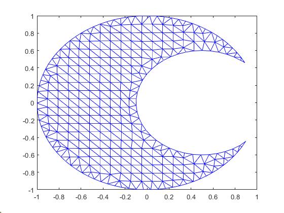
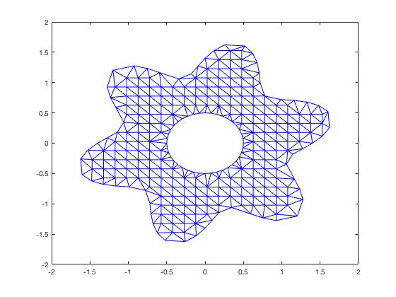
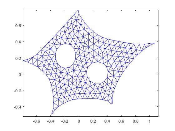
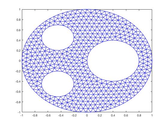
Figure 1: Domains with positive reach

A domain with $C^{2}$ boundary has a positive reach. As Figure 1 illustrates, the domains with positive reach are much more general than convex domains. See Figure 2 for domains with positive reach in the 3D setting. Let $B(0,\epsilon)$ be the closed ball centering at 0 with radius $\epsilon>0,$ and let $K^{c}$ stand for the complement of the set $K\in\mathbb{R}^{d}.$ For any $\epsilon>0,$ the set

$$E_{\epsilon}(K):=(K^{c}+B(0,\epsilon))^{c}\subseteq K$$

is called an $\epsilon$-erosion of $K.$

Definition 2

A set $K\subseteq\mathbb{R}^{d}$ is said to have a uniformly positive reach $r_{0}$ if there exists some $\epsilon_{0}>0$ such that for all $\epsilon\in[0,\epsilon_{0}],E_{\epsilon}(K)$ has a positive reach at least $r_{0}.$

And we have the following property about these domains

Lemma 1

If $\Omega\subset\mathbb{R}^{d}$ is of positive reach $r_{0}$, then for any $0<\epsilon<r_{0}$, the boundary of $\Omega_{\epsilon}:=\Omega+B(0,\epsilon)$ containing $\Omega$ is of $C^{1,1}$. Furthermore, $\Omega_{\epsilon}$ has a positive reach $\geq r_{0}-\epsilon.$

In [5], Gao and Lai proved the following regularity theorem which will be used to prove Theorem 1 in the next section.

Theorem 3

Let $\Omega$ be a bounded domain. Suppose the closure of $\Omega$ is of uniformly positive reach $r_{\Omega}$. For any $f\in L^{2}(\Omega),$ let $u\in H^{1}_{0}(\Omega)$ be the unique weak solution of the Dirichlet problem:

$$\begin{cases}-\Delta u&=f~{}~{}in~{}\Omega\\ u&=0~{}~{}on~{}\partial\Omega\end{cases}$$

Then $u\in H^{2}(\Omega)$ in the sense that

$$\sum_{i,j=1}^{n}\int_{\Omega}(\frac{\partial^{2}u}{\partial x_{i}\partial x_{j}})^{2}\leq C_{0}\int_{\Omega}f^{2}dx$$ (14)

for a positive constant $C_{0}$ depending only on $r_{\Omega}$.

2.2 Multivariate Splines

Next we quickly summarize the essentials of multivariate splines in this subsection. We introduce bivariate spline functions first. Before we start, we first review some facts about triangles. Given a triangle $T$, we write $|T|$ for the length of its longest edge, and $\rho_{T}$ for the radius of the largest disk that can be inscribed in $T$. For any polygonal domain $\Omega\subset\mathbb{R}^{d}$ with $d=2$, let $\triangle:=\{T_{1},\cdots,T_{n}\}$ be a triangulation of $\Omega$ which is a collection of triangles and $\mathcal{V}$ be the set of vertices of $\triangle$. We called a triangulation as a quasi-uniform triangulation if all triangles $T$ in $\triangle$ have comparable sizes in the sense that

$$\frac{|T|}{\rho_{T}}\leq C<\infty,~{}~{}~{}~{}\text{for all triangles}~{}T\in\triangle,$$

where $\rho_{T}$ is the inradius of $T$. Let $|\triangle|$ be the length of the longest edge in $\triangle.$ For a triangle $T=(v_{1},v_{2},v_{3})\in\Omega,$ we define the barycentric coordinates $(b_{1},b_{2},b_{3})$ of a point $(x,y)\in\Omega$. These coordinates are the solution to the following system of equations

$$b_{1}+b_{2}+b_{3}=1$$

$$b_{1}v_{1,x}+b_{2}v_{2,x}+b_{3}v_{3,x}=x$$

$$b_{1}v_{1,y}+b_{2}v_{2,y}+b_{3}v_{3,y}=y$$

where the vertices $v_{i}=(v_{i,x},v_{i,y})$ for $i=1,2,3$ and are nonnegative if $(x,y)\in T.$ We use the barycentric coordinates to define the Bernstein polynomials of degree $D$:

$$B^{T}_{i,j,k}(x,y):=\frac{{D}!}{i!j!k!}b_{1}^{i}b_{2}^{j}b_{3}^{k},~{}i+j+k=D,$$

which form a basis for the space $\mathcal{P}_{D}$ of polynomials of degree $D$. Therefore, we can represent all $s\in S^{-1}_{D}(\triangle)$ in B-form:

$$s|_{T}=\sum_{i+j+k=D}c_{ijk}B^{T}_{ijk},\quad\forall T\in\triangle,$$

where the B-coefficients $c_{i,j,k}$ are uniquely determined by $s$.

Moreover, for given $T=(v_{1},v_{2},v_{3})\in\triangle$, we define the associated set of domain points to be

$$\mathcal{D}_{D,T}:=\{\frac{iv_{1}+jv_{2}+kv_{3}}{D}\}_{i+j+k=D}.$$ (15)

Let $\mathcal{D}_{D,\triangle}=\cup_{T\in\triangle}\mathcal{D}_{D,T}$ be the domain points of triangulation $\triangle$ and degree $D$.

We use the discontinuous spline space $S^{-1}_{D}(\triangle):=\{s|_{T}\in\mathcal{P}_{D},T\in\triangle\}$ as a base. Then we add the smoothness conditions to define the space $\mathcal{S}^{r}_{D}(\triangle):=C^{r}(\Omega)\cap S^{-1}_{D}(\triangle).$ The smoothness conditions are explained in [10]. They are linear equations as seen in Theorems 2.28 and 15.31 in [10]. Let ${\bf c}$ be the coefficient vector of $s\in S^{-1}_{D}(\triangle)$ and $H$ be the matrix which consists of the smoothness conditions across each interior edge of $\triangle$. Then it is known that $H{{\bf c}}=0$ if and only if $s\in C^{r}(\Omega)$ (cf. [10]).

Computations involving splines written in B-form can be performed easily according to [14], [2] and [12]. In fact, these spline functions have numerically stable, closed-form formulas for differentiation, integration, and inner products. If $D\geq 3r+2$, spline functions on quasi-uniform triangulations have optimal approximation power.

Lemma 2

([Lai and Schumaker, 2007[10]]) Let $k\geq 3r+2$ with $r\geq 1$. Suppose $\triangle$ is a quasi-uniform triangulation of $\Omega$. Then for every $u\in W_{q}^{k+1}(\Omega),$ there exists a quasi-interpolatory spline $s_{u}\in\mathcal{S}^{r}_{k}(\triangle)$ such that

$$\|D^{\alpha}_{x}D^{\beta}_{y}(u-s_{u})\|_{q,\Omega}\leq C|\triangle|^{k+1-\alpha-\beta}|u|_{k+1,q,\Omega}$$

for a positive constant $C$ dependent on $u,r,k$ and the smallest angle of $\triangle$, and for all $0\leq\alpha+\beta\leq k$ with

$$|u|_{k,q,\Omega}:=(\sum_{a+b=k}\|D_{x}^{a}D_{y}^{b}u\|^{q}_{L^{q}(\Omega)})^{\frac{1}{q}}.$$

Similarly, for trivariate splines, let $\Omega\subset\mathbb{R}^{3}$ and $\triangle$ be a tetrahedralization of $\Omega$. We define a trivariate spline just like bivariate splines by using Bernstein-Bézier polynomials defined on each tetrahedron $t\in\triangle$. Letting

$$\mathcal{S}^{r}_{D}(\triangle)=\{s\in C^{r}(\Omega):s|_{t}\in\mathbb{P}_{D},t\in\triangle\}=C^{r}(\Omega)\cap S^{-1}_{D}(\triangle)$$

be the spline space of degree $D$ and smoothness $r\geq 0$, each $s\in\mathcal{S}^{r}_{D}(\triangle)$ can be rewritten as

$$s|_{t}=\sum_{i+j+k+\ell=D}c^{t}_{ijk\ell}B^{t}_{ijk\ell},\quad\forall t\in\triangle,$$

where $B^{t}_{ijk\ell}$ are Bernstein-Bézier polynomials (cf. [2], [10], [17] ) which are nonzero on $t$ and zero otherwise. Approximation properties of trivariate splines can be found in [11] and [8].

How to use them to numerically solve partial differential equations based on the weak formulation like the finite element method has been discussed in [2], [17], [12].

3 A Spline Based Collocation Method for the Poisson Equation

For convenience, we simply explain our method when $d=2$ in this section. Numerical results in the settings of $d=2$ and $d=3$ will be given in later sections.

For a given triangulation $\triangle$, we use a spline space $S^{r}_{D}(\triangle)$ to find the coefficient vector c of spline function $\displaystyle s=\sum_{t\in\triangle}\sum_{i+j+k=D}c^{t}_{ijk}B^{t}_{ijk}\in S^{r}_{D}(\triangle)$ satisfying the following equations

$$\left\{\begin{array}[]{cl}\displaystyle-\sum_{t\in\triangle}\sum_{i+j+k=D}c^{t}_{ijk}\Delta B^{t}_{ijk}(\xi_{i})&=f(\xi_{i}),\quad\xi_{i}\in\Omega\subset\mathbb{R}^{2}\cr s(\xi_{i})&=g(\xi_{i}),\quad\hbox{ on }\partial\Omega,\end{array}\right.$$ (16)

where $\{{\xi_{i}}\}_{i=1,\cdots,N}\in\mathcal{D}_{D^{\prime},\triangle}$ are the domain points of $\triangle$ of degree $D^{\prime}$ as explained in (15) in the previous section and $D^{\prime}>D$. Using these points, we have the following matrix equation:

$$-K\textbf{c}:=\begin{bmatrix}-\Delta(B^{t}_{ijk}(\xi_{i}))\end{bmatrix}\textbf{c}=[f(\xi_{i})]=\textbf{f},$$

where c is the vector consisting of all spline coefficients $c^{t}_{ijk},i+j+k=D,t\in\triangle$. In general, the spline $s$ with coefficients in $\bf{c}$ is a discontinuous function. In order to make $s\in\mathcal{S}^{r}_{D}(\triangle)$, its coefficient vector c must satisfy the constraints $H\textbf{c}=0$ for the smoothness conditions that the $\mathcal{S}^{r}_{D}(\triangle)$ functions possess (cf. [10]).

Based on the smoothness conditions (cf. Theorem 2.28 or Theorem 15.38 in [10]), we can construct matrices $H_{0}$ for the $C^{0}$ smoothness conditions of spline functions and $H_{r}$ for the $C^{r}$ smoothness conditions for $r\geq 2$, respectively. Our collocation method is to find ${\bf c}^{*}$ by solving the following constrained minimization:

$$\min_{\bf c}J(c)=\frac{1}{2}(\alpha\|B{\bf c}-{\bf g}\|^{2}+\beta\|H_{r}{\bf c}\|^{2}+\gamma\|H_{0}{\bf c}\|^{2})\quad\text{subject to }\|K{\bf c}+{\bf f}\|\leq\epsilon_{1},$$ (17)

where $B,{\bf g}$ are associated with the boundary condition, $H_{r}$ is associated with the smoothness condition with $r=2$ and $H_{0}$ is associated with the smoothness condition with $r=0$, $\alpha>0,\beta>0,\gamma>0$ are fixed parameters, and $\epsilon_{1}>0$ is a given tolerance. It is easy to see that the minimization (17) is a convex minimization problem over a convex feasible set. The problem (17) will have a unique solution if the feasible set is not empty. We shall use the following iterative method to solve the minimization problem (17). See Appendix for a derivation and a proof of the convergence of Algorithm 1.

Let $I$ be the identity matrix of $\mathbb{R}^{m}$. Fix $\epsilon>0.$ Given an initial guess $\lambda^{(0)}\in\text{Im}(K)$, we first compute

$${\bf z}^{(1)}=(\alpha B^{\top}B+\beta H_{r}^{\top}H_{r}+\gamma H_{0}^{\top}H_{0}+\frac{1}{\epsilon}K^{\top}K)^{-1}(\alpha B^{\top}G+\frac{1}{\epsilon}K^{\top}{\bf f}-K^{\top}\lambda^{(0)})$$

and iteratively compute

$$(\alpha B^{\top}B+\beta H_{r}^{\top}H_{r}+\gamma H_{0}^{\top}H_{0}+\frac{1}{\epsilon}K^{\top}K){\bf z}^{(k+1)}=(\alpha B^{\top}B+\beta H^{\top}H+\gamma H_{0}^{\top}H_{0}){\bf z}^{(k)}+\frac{1}{\epsilon}K^{\top}{\bf f}$$

for $k=1,2,\cdots,$ where $\text{Im}(K)$ is the range of $K.$

Algorithm 1 Iterative Method

Let $u_{s}$ be the solution of Algorithm 1. We would like to show

$$\|u-u_{s}\|_{L^{2}(\Omega)}\leq C|\triangle|^{2}\epsilon_{1}$$ (18)

for some constant $C>0$, where $|\triangle|$ is the size of the underlying triangulation or tetrahedralization $\triangle$ of the domain $\Omega$. To do so, we first show

Lemma 3

Suppose that $\Omega$ is a polygonal domain. Suppose that $u\in H^{3}(\Omega)$. Then there exists a positive constant $\hat{C}$ depending on $D\geq 1$ and $D^{\prime}>D$ such that

$$\|\Delta u(x,y)-\Delta u_{s}(x,y)\|_{L^{2}(\Omega)}\leq\epsilon_{1}\hat{C}.$$

• Proof. Indeed, by Lemma 2, we have a quasi-interpolatory spline $s_{u}$ satisfying

  $$|\Delta u(x,y)-\Delta s_{u}(x,y)|\leq\epsilon,\forall(x,y)\in\Omega$$

  for a triangulation $\triangle$ with $|\triangle|$ small enough. Since $\Delta u(x,y)=-f(x,y)$, we have

  $$\|\Delta s_{u}+{\bf f}\|\leq\epsilon_{1}$$ (19)

  if $\epsilon$ small enough. That is, the feasible set is not empty.

  Next we use the minimization (17) to have the minimizer $u_{s}$ satisfying

  $$|\Delta u(x_{i},y_{i})-\Delta u_{s}(x_{i},y_{i})|\leq\epsilon_{1}$$

  with sufficiently small $|\triangle|$ for any domain points $(x_{i},y_{i})$ which construct the collocation matrix $K$. Now, these two inequalities imply that

  $$|\Delta u_{s}(x_{i},y_{i})-\Delta s_{u}(x_{i},y_{i})|\leq\epsilon_{1}+\epsilon_{1}.$$

  Note that $\Delta u_{s}-\Delta s_{u}$ is a polynomial over each triangle $t\in\triangle$ which has small values at the domain points. This implies that the polynomial $\Delta u_{s}-\Delta s_{u}$ is small over $t$. That is,

  $$|\Delta u_{s}(x,y)-\Delta s_{u}(x,y)|\leq C(\epsilon_{1}+\epsilon_{1})=2C\epsilon_{1}$$ (20)

  by using Theorem 2.27 in [10]. Finally, we can use (20) to prove

  $$|\Delta u(x,y)-\Delta u_{s}(x,y)|=|\Delta u(x,y)-\Delta s_{u}(x,y)+\Delta s_{u}(x,y)-\Delta u_{s}(x,y)|\leq\epsilon_{1}+2C\epsilon_{1}.$$

  and then

  $$\|\Delta u(x,y)-\Delta u_{s}(x,y)\|_{L^{2}(\Omega)}\leq\epsilon_{1}\hat{C}$$

  for a constant $\hat{C}$ depending on the bounded domain $\Omega$ and $D,D^{\prime}$, but independent of $|\triangle|$. $\Box$

Now, let us consider the convergence of our method. Without loss of generality, we may assume $g=0$. Indeed, for any general $g$, let $u_{g}\in H^{2}(\Omega)$ be a function satisfying the boundary condition, i.e. $u_{g}|_{\partial\Omega}=g$ and we consider the Poisson equation with solution $w=u-u_{g}$ and the new right-hand side $f_{w}=f+\Delta u_{g}$. Recall the standard norm on $H^{2}(\Omega)$ defined in (3). It is also a norm of $H^{2}(\Omega)\cap H^{1}_{0}(\Omega)$. It is easy to see that the space $H^{2}(\Omega)\cap H^{1}_{0}(\Omega)$ is a Banach space with the norm $\|\cdot\|_{H^{2}(\Omega)}$. In addition, let us define a new norm $\|u\|_{L}$ on $H^{2}(\Omega)\cap H^{1}_{0}(\Omega)$ as follows.

$$\|u\|_{L}=\|\Delta u\|_{L^{2}(\Omega)}$$ (21)

We can easily show that $\|\cdot\|_{L}$ is a norm on $H^{2}(\Omega)\cap H^{1}_{0}(\Omega)$ as follows: Indeed, if $\|u\|_{L}=0$, then $\Delta u=0$ in $\Omega$ and $u=0$ on the boundary $\partial\Omega$. By the Green theorem, we get

$$\int_{\Omega}|\nabla u|^{2}=-\int_{\Omega}u\Delta u+\int_{\partial\Omega}u\frac{\partial u}{\partial n}=0.$$

By Poincaré’s inequality, we get

$$\|u\|_{L^{2}(\Omega)}\leq C\|\nabla u\|_{L^{2}(\Omega)}=0.$$

Hence, we know that $u=0.$ Next for any scalar $a$, it is trivial to have

$$\|au\|_{L}=\|\Delta(au)\|_{L^{2}(\Omega)}=|a|\|\Delta u\|_{L^{2}(\Omega)}=|a|\|u\|_{L}.$$

Finally, the triangular inequality is also trivial.

$$\|u+v\|_{L} = \|\Delta(u+v)\|_{L^{2}(\Omega)}\leq\|\Delta u\|_{L^{2}(\Omega)}+\|\Delta v\|_{L^{2}(\Omega)}=\|u\|_{L}+\|v\|_{L}$$

by linearity of the Laplacian operator.

We now show that the new norm is equivalent to the standard norm on $H^{2}(\Omega)\cap H^{1}_{0}(\Omega)$. We are now ready to establish the following

Theorem 4

Suppose $\Omega\subset\mathbb{R}^{d}$ is a bounded domain and the closure of $\Omega$ is of uniformly positive reach $r_{\Omega}>0$. There exist two positive constants $A$ and $B$ such that

$$A\|u\|_{H^{2}}\leq\|u\|_{L}\leq B\|u\|_{H^{2}},\quad\forall u\in H^{2}(\Omega)\cap H^{1}_{0}(\Omega).$$ (22)

• Proof. We first show that $H^{2}(\Omega)\cap H^{1}_{0}(\Omega)$ is the Banach space with the norm $\|u\|_{L}$. Assume that $\{u_{n}\}$ is the Cauchy sequence in $H^{2}(\Omega)\cap H^{1}_{0}(\Omega)$. We know that $\{\Delta u_{n}\}$ is a Cauchy sequence in $L^{2}(\Omega)$. Then there exists $U^{*}\in L^{2}(\Omega)$ such that $\Delta u_{n}$ converges to $U^{*}.$ It is known there exist a unique $u^{*}$ satisfying the Dirichlet problem:

  $$\begin{cases}\Delta u&=U^{*}\\ u&=0.\end{cases}$$

  By Theorem 3, we know $u^{*}\in H^{2}(\Omega)\cap H^{1}_{0}(\Omega)$. Thus, we can say that there exist the unique $u^{*}$ satisfying $\|u_{n}-u^{*}\|_{L}\rightarrow 0$ as $n\rightarrow\infty$. It is easy to get the following inequality

  $$\|u\|_{L} = \|\Delta u\|_{L^{2}(\Omega)}\leq\sum_{i,j=1}^{d}\|\frac{\partial^{2}}{\partial x_{i}\partial x_{j}}u\|_{L^{2}(\Omega)}\leq\|u\|_{H^{2}}$$ (23)

  for all $u\in H^{2}(\Omega)\cap H^{1}_{0}(\Omega)$.

  Next, by Theorem 3, more precisely, by (14), we have

  $$\|u\|_{H^{2}}\leq C\|\Delta u\|_{L^{2}(\Omega)}=C\|u\|_{L}$$

  for a constant $C$ dependent on $C_{0}$ in (14). Therefore, we choose $A=\frac{1}{C}$ to finish the proof. $\Box$

Using Theorem 4, we immediately obtain the following theorem

Theorem 5

Suppose $f$ and $g$ are continuous over bounded domain $\Omega\subseteq\mathbb{R}^{d}$ for $d\geq 2$. Suppose $\Omega\subset\mathbb{R}^{d}$ be a bounded domain and the closure of $\Omega$ is of uniformly positive reach $r_{\Omega}>0$. Suppose that $u\in H^{3}(\Omega)$ and $(u-u_{s})|_{\partial\Omega}=0$. We have the following inequality

$$\|u-u_{s}\|_{L^{2}(\Omega)}\leq C\epsilon_{1},\|\nabla(u-u_{s})\|_{L^{2}(\Omega)}\leq C\epsilon_{1}$$

and

$$\sum_{i+j=2}\|\frac{\partial^{2}}{\partial x^{i}\partial y^{j}}u\|_{L^{2}(\Omega)}\leq C\epsilon_{1}$$

for a positive constant $C$ depending on $A$ and $\Omega$, where $A$ is one of the constants in Theorem 4.

• Proof. Using Lemma 3 and the assumption on the approximation on the boundary, we have

  $$\|u-u_{s}\|_{H^{2}(\Omega)} \leq\frac{1}{A}\|\Delta(u-u_{s})\|_{L^{2}(\Omega)}\leq\frac{1}{A}\epsilon_{1}\hat{C}.$$

  We choose $C=\frac{\hat{C}}{A}$ to finish the proof. $\Box$

Finally we show that the convergence of $\|u-u_{s}\|_{L^{2}(\Omega)}$ and $\|\nabla(u-u_{s})\|_{L^{2}(\Omega)}$ can be better.

Theorem 6

Suppose that $(u-u_{s})|_{\partial\Omega}=0$. Under the assumptions in Theorem 5, we have the following inequality

$$\|u-u_{s}\|_{L^{2}(\Omega)}\leq C|\triangle|^{2}\epsilon_{1}\hbox{ and }\|\nabla(u-u_{s})\|_{L^{2}(\Omega)}\leq C|\triangle|\epsilon_{1}$$

for a positive constant $C=1/A$, where $A$ is one of the constants in Theorem 4 and $|\triangle|$ is the size of the underlying triangulation $\triangle$.

• Proof. First of all, it is known for any $w\in H^{2}(\Omega)\cap H^{1}_{0}(\Omega)$, there is a continuous linear spline $L_{w}$ over the triangulation $\triangle$ such that

  $$\|D_{x}^{\alpha}D_{y}^{\beta}(w-L_{w})\|_{L^{2}(\Omega)}\leq C|\triangle|^{2-\alpha-\beta}|w|_{H^{2}(\Omega)}$$ (24)

  for nonnegative integers $\alpha\geq 0,\beta\geq 0$ and $\alpha+\beta\leq 2$, where $|w|_{H^{2}(\Omega)}$ is the semi-norm of $w$ in $H^{2}(\Omega)$. Indeed, we can use the same construction method for quasi-interpolatory splines used for the proof of Lemma 2 to establish the above estimate. The above estimate will be used twice below.

  By the assumption that $u-u_{s}=0$ on $\partial\Omega$, it is easy to see

  $$\|\nabla(u-u_{s})\|^{2}_{L^{2}(\Omega)}=-\int_{\Omega}\Delta(u-u_{s})(u-u_{s})=-\int_{\Omega}\Delta(u-u_{s}-L_{u-u_{s}})(u-u_{s})$$

  $$= \int_{\Omega}\nabla(u-u_{s}-L_{u-u_{s}})\nabla(u-u_{s})\leq\|\nabla(u-u_{s})\|_{L^{2}(\Omega)}\|\nabla(u-u_{s}-L_{u-u_{s}})\|_{L^{2}(\Omega)}$$

  $$\leq \|\nabla(u-u_{s})\|_{L^{2}(\Omega)}C|\triangle|\cdot|u-u_{s}|_{H^{2}(\Omega)}$$

  $$\leq \|\nabla(u-u_{s})\|_{L^{2}(\Omega)}|\triangle|\frac{C}{A}\|\Delta(u-u_{s})\|_{L^{2}(\Omega)}.$$

  where we have used the first inequality in Theorem 4. It follows that $\|\nabla(u-u_{s})\|_{L^{2}(\Omega)}\leq|\triangle|\frac{C}{A}\epsilon_{1}$.

  Next we let $w\in H^{2}(\Omega)\cap H^{1}_{0}(\Omega)$ be the solution to the following Poisson equation:

  $$\left\{\begin{array}[]{cl}-\Delta w&=u-u_{s}~{}~{}~{}\text{in}~{}\Omega\subset\mathbb{R}^{d}\\ w&=0~{}~{}~{}\text{on}~{}\partial\Omega,\end{array}\right.$$ (25)

  Then we use the continuous linear spline $L_{w}$ to have

  $$\|u-u_{s}\|^{2}_{L^{2}(\Omega)} = -\int_{\Omega}\Delta w(u-u_{s})=-\int_{\Omega}\Delta(w-L_{w})(u-u_{s})$$

  $$= \int_{\Omega}\nabla(w-L_{w})\nabla(u-u_{s})\leq\|\nabla(u-u_{s})\|_{L^{2}(\Omega)}\|\nabla(w-L_{w})\|_{L^{2}(\Omega)}$$

  $$\leq \|\nabla(u-u_{s})\|_{L^{2}(\Omega)}C|\triangle|\cdot|w|_{H^{2}(\Omega)}\leq\frac{C}{A}|\triangle|\epsilon_{1}|\triangle|\frac{C}{A}\|\Delta w\|_{L^{2}(\Omega)}$$

  $$= \frac{C}{A}|\triangle|\epsilon_{1}|\triangle|\frac{C}{A}\|u-u_{s}\|_{L^{2}(\Omega)}.$$

  where we have used the first inequality in Theorem 4 and the estimate of $\|\nabla(u-u_{s})\|_{L^{2}(\Omega)}$ above. Hence, we have $\|u-u_{s}\|_{L^{2}(\Omega)}\leq\frac{C^{2}}{A^{2}}|\triangle|^{2}\epsilon_{1}$ as $|\triangle|\to 0$. $\Box$

4 General Second Order Elliptic Equations

In this section we consider a collocation method based on bivariate/trivariate splines for a solution of the general second order elliptic equation in (2). For the PDE coefficient functions $a^{ij},b^{i},c^{1}\in L^{\infty}(\Omega)$, we assume that

$$a_{ij}=a_{ji}\in L^{\infty}(\Omega)~{}~{}\forall i,j=1,\cdots,d$$ (26)

and there exist $\lambda,\Lambda$ such that

$$\lambda\sum_{i=1}^{d}\eta_{i}^{2}\leq\sum_{i,j}^{d}a^{ij}(x)\eta_{i}\eta_{j}\leq\Lambda\sum_{i=1}^{d}\eta_{i}^{2},\forall\eta\in\mathbb{R}^{d}\backslash\{0\}$$ (27)

for all $i,j$ and $x\in\Omega$. For convenience, we first assume that $b^{i}{=}0$ and $c^{1}=0$ in this section. In addition to the elliptic condition, we add the Cordés condition for well-posedness of the problem. We assume that there is an $\epsilon\in(0,1]$ such that

$$\frac{\sum_{i,j=1}^{d}(a^{i,j})^{2}}{(\sum_{i=1}^{d}a^{ii})^{2}}\leq\frac{1}{d-1+\epsilon}~{}~{}a.e.~{}in~{}\Omega$$ (28)

Next let $\theta\in L^{\infty}(\Omega)$ be defined by

$$\theta:=\frac{\sum_{i=1}^{d}a^{ii}}{\sum_{i,j=1}^{d}(a^{i,j})^{2}}.$$

Under these conditions, the researchers in [19] proved the following lemma

Lemma 4

Let the operator $\mathcal{L}(u):=\sum_{i,j=1}^{d}a^{ij}(x)\frac{\partial^{2}}{\partial x_{i}\partial x_{j}}u$ satisfy (26), (27) and (28). Then for any open set $U\subseteq\Omega$ and $v\in H^{2}(U)$, we have

$$|\theta\mathcal{L}v-\Delta v|\leq\sqrt{1-\epsilon}|D^{2}v|~{}~{}a.e.~{}in~{}U,$$ (29)

where $\epsilon\in(0,1]$ is as in (28).

Instead of using the convexity to ensure the existence of the strong solution of (2) in [19], we shall use the concept of uniformly positive reach in [5]. The following is just the restatement of Theorem 3.3 in [5].

Theorem 7

Suppose that $\Omega\subset\mathbb{R}^{d}$ with $d\geq 2$ is a bounded domain with uniformly positive reach. Then the second order elliptic PDE in (2) satisfying (28) has a unique strong solution in $H^{2}(\Omega)$.

We now extend the collocation method in the previous section to find a numerical solution of (2). Similar to the discussion in the previous section, we can construct the following matrix for the PDE in (2):

$$\mathcal{K}:=\begin{bmatrix}\sum_{i,j=1}^{d}a^{ij}(\xi_{i})\frac{\partial^{2}}{\partial x_{i}\partial x_{j}}(B^{t}_{ijk}(\xi_{i}))\end{bmatrix}.$$

Similar to (17), consider the following minimization problem:

$$\min_{\bf c}J(c)=\frac{1}{2}(\alpha\|B{\bf c}-{\bf g}\|^{2}+\beta\|H{\bf c}\|^{2}+\gamma\|H_{0}{\bf c}\|^{2})\quad\text{subject to }-\mathcal{K}{\bf c}={\bf f},$$ (30)

Again we will solve a nearby minimization problem as in the previous section. Like the Poisson equation, we let $\epsilon_{1}=\|\mathcal{K}{\bf c}+{\bf f}\|$ for the minimizer ${\bf c}$ of (30). To study the convergence, we may assume that $g=0$ as in the previous section so that the solution $u_{s}$ with the coefficient vector ${\bf c}$ which is the minimizer of (30) satisfies $u_{s}=0$ on $\partial\Omega$ and hence, $\|u-u_{s}\|_{L^{2}(\partial\Omega)}=0$. Also, we have that $\|\mathcal{L}u_{s}+f\|_{L^{2}(\Omega)}\leq\epsilon_{1}$.

To show $u_{s}$ approximate $u$ over $\Omega$, let us define a new norm $\|u\|_{\mathcal{L}}$ on $H^{2}(\Omega)\cap H^{1}_{0}(\Omega)$ as follows.

$$\|u\|_{\mathcal{L}}=\|\mathcal{L}u\|_{L^{2}(\Omega)}$$ (31)

We can show that $\|\cdot\|_{\mathcal{L}}$ is a norm on $H^{2}(\Omega)\cap H^{1}_{0}(\Omega)$ as follows if $\epsilon\in(0,1]$ is large enough. Indeed, if $\|u\|_{\mathcal{L}}=0$, then $\mathcal{L}u=0$ in $\Omega$ and $u=0$ on the boundary $\partial\Omega$. Using this Lemma 4 and Theorem 4, we get

$$\int_{\Omega}\Delta u\Delta u-\int_{\Omega}(\Delta-\theta\mathcal{L})u\Delta u=\int_{\Omega}\theta\mathcal{L}(u)\Delta u=0$$ (32)

and

$$\int_{\Omega}\Delta u\Delta u-\int_{\Omega}(\Delta-\theta\mathcal{L})u\Delta u\geq\int_{\Omega}|\Delta u|^{2}-\int_{\Omega}\sqrt{1-\epsilon}|D^{2}u|\cdot|\Delta u|$$

$$=\int_{\Omega}|\Delta u|^{2}-\int_{\Omega}\sqrt{1-\epsilon}|D^{2}u|\cdot|\Delta u|\geq\|\Delta u\|^{2}-\frac{\sqrt{1-\epsilon}}{A}\|\Delta u\|\|\Delta u\|.$$

Therefore, if $\epsilon>1-A^{2}$, then

$$(1-\frac{\sqrt{1-\epsilon}}{A})\|\Delta u\|\leq 0.$$

Hence, we know that $u=0.$ The other two properties of the norm can be proved easily.

We mainly show that the above norm is equivalent to the standard norm on $H^{2}(\Omega)\cap H^{1}_{0}(\Omega)$. Indeed, recall a well-known property about the norm equivalence.

Lemma 5

([Brezis, 2011 [3]]) Let $E$ be a vector space equipped with two norms, $\|\cdot\|_{1}$ and $\|\cdot\|_{2}$. Assume that $E$ is a Banach space for both norms and that there exists a constant $C>0$ such that

$$\|x\|_{2}\leq C\|x\|_{1},~{}\forall x\in E.$$ (33)

Then the two norms are equivalent, i.e., there is a constant $c>0$ such that

$$\|x\|_{1}\leq c_{1}\|x\|_{2},~{}\forall x\in E.$$

• Proof. We define $E_{1}=(E,\|\cdot\|_{1})$ and $E_{2}=(E,\|\cdot\|_{2})$ be two spaces equipped with two different norms. It is easy to see that $E_{1}$ and $E_{2}$ are Banach spaces. Let $I$ be the identity operator which maps any u in $E_{1}$ to $u$ in $E_{2}$. Clearly, it is an injection and onto because of the identity mapping and hence, it is a surjection. Because of (33), the mapping $I$ is a continuous operator. Now we can use the well-known open mapping theorem. Let $B_{1}(0,1)=\{u\in E_{1},\|u\|_{1}\leq 1\}$ be an open ball. The open mapping theorem says that $I(B_{1}(0,1))$ is open and hence, it contains a ball $B_{2}(0,c)=\{u\in E_{2},\|u\|_{2}<c\}$. That is, $B_{2}(0,c)\subset I(B_{1}(0,1))$. Let us claim that $c\|u\|_{1}\leq\|I(u)\|_{2}$ for all $u\in E_{1}$. Otherwise, there exists a $u^{*}$ such that $c\|u^{*}\|_{1}>\|I(u^{*})\|_{2}$. That is, $c>\|I(u^{*}/\|u^{*}\|_{1})\|_{2}$. So $I(u^{*}/\|u^{*}\|_{1})\in B_{2}(0,c)$. There is a $u^{**}\in B_{1}(0,1)$ such that $Iu^{**}=I(u^{*}/\|u^{*}\|_{1})$. Since $I$ is an injection, $u^{**}=I(u^{*}/\|u^{*}\|_{1}$. Since $u^{**}\in B_{1}(0,1)$, we have $1>\|u^{**}\|_{1}=\|(u^{*}/\|u^{*}\|_{1}))\|=1$ which is a contradiction. This shows that the claim is correct. we have thus $c\|u\|_{1}\leq\|I(u)\|_{2}=\|u\|_{2}$ for all $u\in E_{1}$. We choose $c_{1}=1/c$ to finish the proof. $\Box$

Using Lemma 5, we can prove the following theorem

Theorem 8

Suppose that $\Omega$ is bounded and has uniformly positive reach $r_{\Omega}>0$ . Then there exist two positive constants $A_{1}$ and $B_{1}$ such that

$$A_{1}\|u\|_{H^{2}(\Omega)}\leq\|u\|_{\mathcal{L}}\leq B_{1}\|u\|_{H^{2}(\Omega)},\quad\forall u\in H^{2}(\Omega)\cap H^{1}_{0}(\Omega).$$ (34)

• Proof. It follows that

  $$\|u\|_{\mathcal{L}} \leq \max_{i,j=1\cdots,d}\|a^{ij}\|_{\infty}\sum_{i,j=1}^{d}\|\frac{\partial^{2}}{\partial x_{i}\partial x_{j}}u\|_{L^{2}(\Omega)}\leq B_{1}\|u\|_{H^{2}(\Omega)}$$

  for all $u\in H^{2}(\Omega)\cap H^{1}_{0}(\Omega)$, where $B_{1}$ depending on $d,\Lambda$ and $C$. Using Lemma 4 and the above inequality, there exist $\alpha_{1}>0$ satisfying

  $$\|u\|_{H^{2}}\leq\alpha_{1}\|u\|_{\mathcal{L}}.$$

  Therefore, we choose $A_{1}=\frac{1}{\alpha_{1}}$ to finish the proof. $\Box$

Theorem 9

Let $\Omega$ be a bounded and closed set satisfying the uniformly positive reach condition. Assume that $a^{ij}\in L^{\infty}(\Omega)$ satisfy (26), (27) and (28) and $\epsilon>1-A^{2}$. Suppose that $u\in H^{3}(\Omega)$ and $u-u_{s}=0$ on $\partial\Omega$. For the solution $u$ of equation (11) and the corresponding minimizer $u_{s}$, we have the following inequality

$$\|u-u_{s}\|_{L^{2}(\Omega)}\leq C\epsilon_{1}$$

for a positive constant $C$ depending on $\Omega$ and $A_{1}$ which is one of the constants in Theorem 8. Similar for $\|\nabla(u-u_{s})\|_{L^{2}(\Omega)}$ and $|u-u_{s}|_{H^{2}}$.

Next we consider the case that $b^{i}$ and $c^{1}$ are not zero. Assume that $\|a^{ij}\|_{\infty}$, $\|b^{i}\|_{\infty}$, $\|c^{1}\|_{\infty}\leq\Lambda_{1}$ and we denote that $\mathcal{L}_{1}(u):=\sum_{i,j=1}^{d}a^{ij}(x)\frac{\partial^{2}}{\partial x_{i}\partial x_{j}}u+\sum_{i=1}^{d}b^{i}(x)\frac{\partial}{\partial x_{i}}u+c^{1}(x)u$ and define a new norm $\|u\|_{\mathcal{L}_{1}}$ on $H^{2}(\Omega)\cap H^{1}_{0}(\Omega)$ as follows.

$$\|u\|_{\mathcal{L}_{1}}=\|\mathcal{L}_{1}u\|_{L^{2}(\Omega)}.$$ (35)

Assume that $\|u\|_{\mathcal{L}_{1}}=0$, i.e., $\mathcal{L}_{1}u=0$ over $\Omega$ and $u=0$ on $\partial\Omega$. From (29), we have

$$\int_{\Omega}\theta\mathcal{L}(u)\Delta u\geq\|\Delta u\|^{2}-\frac{\sqrt{1-\epsilon}}{A}\|\Delta u\|^{2}.$$

Then by the above inequality we get

$$0 = \int_{\Omega}\theta\mathcal{L}_{1}(u)\Delta u=\int_{\Omega}\theta\mathcal{L}(u)\Delta u+\sum_{i=1}^{d}\theta b^{i}(x)\frac{\partial}{\partial x_{i}}u\Delta u+\theta c^{1}(x)u\Delta u$$

$$\geq \|\Delta u\|^{2}-\frac{\sqrt{1-\epsilon}}{A}\|\Delta u\|^{2}+\int_{\Omega}\sum_{i=1}^{d}\theta b^{i}(x)\frac{\partial}{\partial x_{i}}u\Delta u+\theta c^{1}(x)u\Delta u$$

$$\geq \|\Delta u\|_{L^{2}(\Omega)}^{2}-\frac{\sqrt{1-\epsilon}}{A}\|\Delta u\|_{L^{2}(\Omega)}^{2}-\|\theta\|_{\infty}\max_{i}\|b^{i}\|_{\infty}\sqrt{d}\|\nabla u\|_{L^{2}(\Omega)}\|\Delta u\|_{L^{2}(\Omega)}$$

$$-\|\theta\|_{\infty}\|c^{1}\|_{\infty}\|u\|_{L^{2}(\Omega)}\|\Delta u\|_{L^{2}(\Omega)}$$

$$= \|\Delta u\|_{L^{2}(\Omega)}^{2}-\frac{\sqrt{1-\epsilon}}{A}\|\Delta u\|_{L^{2}(\Omega)}^{2}-C_{m}(\|\nabla u\|_{L^{2}(\Omega)}\|\Delta u\|_{L^{2}(\Omega)}+\|u\|_{L^{2}(\Omega)}\|\Delta u\|_{L^{2}(\Omega)}),$$

where $C_{m}=\max\{\|\theta\|_{\infty}\max_{i}\|b^{i}\|_{\infty}\sqrt{d},\|\theta\|_{\infty}\|c^{1}\|_{\infty}\}$. Dividing $\|\Delta u\|_{L^{2}(\Omega)}$ both sides of the inequality above and using Theorem 1, it is followed that

$$0 \geq \|\Delta u\|_{L^{2}(\Omega)}-\frac{\sqrt{1-\epsilon}}{A}\|\Delta u\|_{L^{2}(\Omega)}-C_{m}(\|\nabla u\|_{L^{2}(\Omega)}+\|u\|_{L^{2}(\Omega)})$$

$$\geq \|\Delta u\|_{L^{2}(\Omega)}-\frac{\sqrt{1-\epsilon}}{A}\|\Delta u\|_{L^{2}(\Omega)}-C_{m}\|u\|_{H^{2}(\Omega)}$$

$$\geq \|\Delta u\|_{L^{2}(\Omega)}-\frac{\sqrt{1-\epsilon}}{A}\|\Delta u\|_{L^{2}(\Omega)}-\frac{C_{m}}{A}\|\Delta u\|_{L^{2}(\Omega)}$$

$$= \|\Delta u\|_{L^{2}(\Omega)}(1-\frac{\sqrt{1-\epsilon}}{A}-\frac{C_{m}}{A}).$$

If the constant $(1-\frac{\sqrt{1-\epsilon}}{A}-\frac{C_{m}}{A})$ is positive, then we can conclude that $\Delta u=0$. Together with the fact $u=0$ on $\partial\Omega$, we know $u=0$. The other properties $\|u+v\|_{\mathcal{L}_{1}}\leq\|u\|_{\mathcal{L}_{1}}+\|v\|_{\mathcal{L}_{1}}$ and $\|au\|_{\mathcal{L}_{1}}=|a|\|u\|_{\mathcal{L}_{1}}$ can be easily proved. The detail is omitted.

Theorem 10

Assume that $(1-\frac{\sqrt{1-\epsilon}}{A}-\frac{C_{m}}{A})>0$. There exist two positive constants $A_{2}$ and $B_{2}$ such that

$$A_{2}\|u\|_{H^{2}(\Omega)}\leq\|u\|_{\mathcal{L}_{1}}\leq B_{2}\|u\|_{H^{2}(\Omega)},\quad\forall u\in H^{2}(\Omega)\cap H^{1}_{0}(\Omega).$$ (36)

• Proof. The proof can be done by using Lemma 5. We leave it to the interested reader. $\Box$

Therefore, we can get the following theorem for the general elliptic PDE:

Theorem 11

Suppose $\Omega\subset\mathbb{R}^{d}$ be a bounded domain and the closure of $\Omega$ is of uniformly positive reach $r_{\Omega}>0$. Assume that $a^{ij},b^{i},c^{1}\in L^{\infty}(\Omega)$ satisfy (26), (27), (28) and $(1-\frac{\sqrt{1-\epsilon}}{A}-\frac{C_{m}}{A})>0$. Suppose that $u\in H^{3}(\Omega)$ and $u-u_{s}=0$ on $\partial\Omega$. For the solution $u$ of equation (2) and the corresponding minimizer $u_{s}$, we have the following inequality

$$\|u-u_{s}\|_{L^{2}(\Omega)}\leq C\epsilon_{1}$$

for a positive constant $C$ depending on $\Omega$ and a constant $A_{2}$ in Theorem 10.

Finally we show that the convergence of $\|u-u_{s}\|_{L^{2}(\Omega)}$ and $\|\nabla(u-u_{s})\|_{L^{2}(\Omega)}$ can be better

Theorem 12

Suppose that the bounded domain $\Omega$ has an uniformly positive reach. Suppose $f$ and $g$ are continuous over bounded domain $\Omega\subseteq\mathbb{R}^{d}$ for $d=2,3$. Let $u$ be the solution of the general second order PDE (2) with differential operator ${\cal L}$. Suppose that $u\in H^{3}(\Omega)$. If $u-u_{s}|_{\partial\Omega}=0$, we further have the following inequality

$$\|u-u_{s}\|_{L^{2}(\Omega)}\leq C|\triangle|^{2}\epsilon_{1}\hbox{ and }\|\nabla(u-u_{s})\|_{L^{2}(\Omega)}\leq C|\triangle|\epsilon_{1}$$

for a positive constant $C=1/A_{2}$, where $A_{2}$ is one of the constants in Theorem 4 and $|\triangle|$ is the size of the underlying triangulation $\triangle$.

• Proof. The proof is similar to Theorem 6. We leave the detail to the interested reader. $\Box$

5 Implementation of the Spline based Collocation Method

Before we present our computational results for Poisson equation and general second order elliptic equations, let us first explain the implementation of our spline based collocation method. We divide the implementation into two parts. The first part of the implementation is to construct the collocation matrices $K$ associated with the Poisson equation and $\mathcal{K}$ associated with the general second order PDE in the non-divergence form over triangulation/tetrahedralization, based the degree $D$ of spline functions and the smoothness $r\geq 1$ as well as the domain points ${\cal D}_{D^{\prime},\triangle}$ associated with the triangulation/tetrahedralization. This part also generates the smoothness matrix $H_{r},H_{0}$. More precisely, for the Poisson equation, we construct collocation matrices

$$MxxV:=[(B_{ijk}^{t}({\bf x})_{xx}|_{{\bf x}=\xi_{\ell}},\xi_{\ell}\in{\cal D}_{D^{\prime},\triangle}]\hbox{ and }MyyV:=[(B_{ijk}^{t}({\bf x})_{yy}|_{{\bf x}=\xi_{\ell}},\xi_{\ell}\in{\cal D}_{D^{\prime},\triangle}].$$ (37)

In fact we choose many other points which are in addition to the domain points to build these $MxxV$ and $MyyV$ to get better accuracy. For example, we choose $D^{\prime}=D+3$ to generate domain points. Then $K=MxxV+MyyV$ is a size of $M\times m$ for the Poisson equation, where $m=\dim(S^{-1}_{D}(\triangle))$ and $M=\dim(S^{-1}_{D^{\prime}}(\triangle))$. After generating matrices, we save our matrices which will be used later for solution of the Poisson equation for various right-hand side functions and various boundary conditions.

For the general elliptic equations, we also generate all the related matrices $MxxV$, $MxyV$, $MyyV$, $MxV,MyV,\cdots$ similar to the matrices $MxxV,MyyV$ for the Poisson equation. Then we generate the collocation matrix $\mathcal{K}$ associated with the PDE coefficients at the same domain points from all the related matrices $MxxV,MxyV,MyyV,MxV,MyV,\cdots$ which are just generated before. This part is the most time consuming step. See Tables 1 and  2 for the 2D and 3D settings.

The second part, Part 2 is to construct the right-hand side vector ${\bf f}$ for each given PDE problem and the matrix $B$ and vector $G$ associated with the boundary condition and use Algorithm 1 to solve the minimization problem (17) and (30). We shall use the four different domains in 2D shown in Fig. 1 and four different domains in 3D shown in Fig. 2 to test the performance of our collocation method. In addition, the spline based collocation method has been tested over many more domains of interest. In particular, many domains which may not be of positive reach are used for testing and their numerical results can be found in [15].

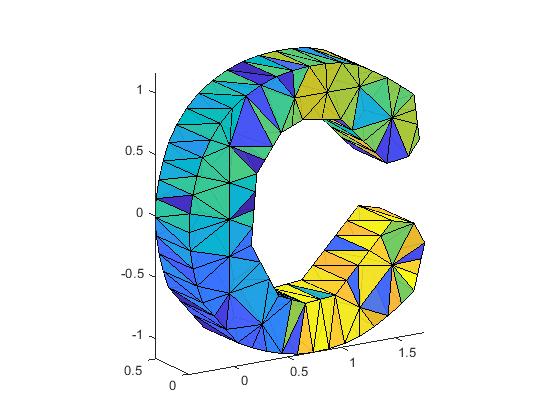
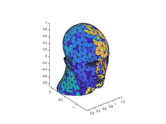
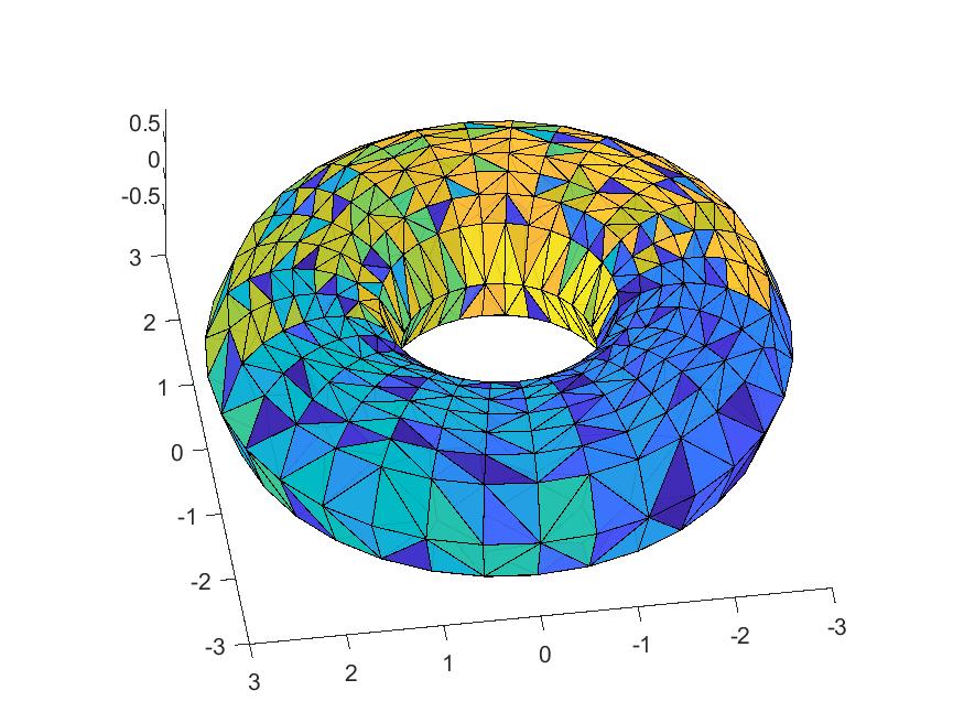
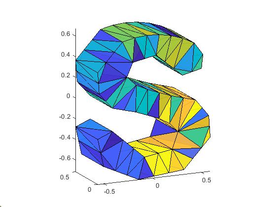
Figure 2: Several 3D domains used for Numerical Experiments

In our computational experiments, we use a cluster computer at University of Georgia to generate the related collocation matrices for various degree of splines and domain points as described in Part I. We use multiple CPUs in the computer so that multiple operations can be done simultaneously. For the 2D case, we use 10 processors on a parallel computer equipped with a 12th Gen Intel(R) Core(TM) i7-12650H processor running at 2.30 GHz and 16.0 GB of installed RAM for both Part 1 and Part 2. And we also use a high memory (512GB) node from the Sapelo 2 cluster at University of Georgia, which has four AMD Opteron 6344 2.6 GHz processors. Using 48 processors on the UGA cluster, we can generate our necessary matrices and the computational times for Part 1 are listed in Table 1. For 3D case, we use 48 processors for Part 1 and 12 processors for Part 2 to do the computation. Tables 2 and  3 show the computational times for generating collocation matrices, where (P), (UGA P) indicates the time for the Poisson equation with 10 processors and 48 processors respectively and (G), (UGA G) for the general second order PDE using 10 processors and 48 processors, respectively.

Domains	Number of	Number of	degree	Time	Time	Time	Time
	vertices	triangles		(P)	(G)	(UGA P)	(UGA G)
Moon	325	531	8	0.48	4.51	1.23	1.80
Flower	297	494	8	0.38	2.47	0.28	0.72
Star	231	366	8	0.30	1.49	0.30	0.71
Circle	525	895	8	0.85	5.83	0.32	1.86

Table 1: Times in seconds for generating necessary matrices for each 2D domain in Figure 1.

Domains	Number of	Number of	Degree of	Time	Time	Time	Time
	vertices	tetrahedron	splines	(P)	(G)	(UGA P)	(UGA G)
Letter C	190	431	9	5.9	69.0	3.17	15.8
Letter S	115	171	9	2.4	25.8	0.72	5.37
Torus	773	2911	9	41.0	451.0	8.39	82.0
Human head	913	1588	9	21.9	243.3	4.53	44.7

Table 2: Times in seconds for generating necessary matrices for each 3D domain in Figure 2.

Domain	Time	Time	Time	Time
	(P)	(SG)	(NSG1)	(NSG2)
Letter C	3.71	6.04	6.07	5.88
Letter S	2.10	2.41	2.33	2.44
Torus	402.13	595.74	285.42	181.83
Human head	27.21	48.10	48.96	48.96

Table 3: Times in seconds for finding solutions of 3D Poisson equation(P), general second order elliptic equation with smooth PDE coefficients (SG) or with non-smooth PDE coefficients (NSG1, NSG2) for each domain in Figure 2.

Another issue of our computation is how to choose $\alpha,\beta,$ and $\gamma$ in our Algorithm 1. As there are many numerical solutions, we need to decide which one to choose. That is, if we are interested more in the accuracy of numerical solutions than the smoothness of the spline solutions, we use $\alpha\geq 100$ while $\beta=\gamma=1$. On the other hand, if we are interested more in the smoothness of spline solutions, e.g. in the computer aided geometric design, we use $\alpha=1$ while $\beta=\gamma\geq 10^{5}$ or $\beta=1$ and $\gamma=10^{5}$. Let us present Figure 3 and 4 to show these phenomena. The numerical results in Figure 3 and 4 are based on spline functions of degree $D=8$ and smoothness $r=2$ over one of four domains in Figure 1 for all the testing functions listed in the next subsection. In this sections, the errors are computed based on $NI=1001\times 1001$ equally-spaced points $\{(\eta_{i})\}_{i=1}^{NI}$ fell inside the different domains. Considered the errors have been calculated according to the norms

$$\begin{cases}|u|_{l_{2}}&=\sqrt{\frac{\sum_{i=1}^{NI}(u(i))^{2}}{NI}}\cr|u|_{h_{1}}&=\sqrt{\frac{\sum_{i=1}^{NI}(u(i))^{2}+(u_{x}(i))^{2}+(u_{y}(i))^{2}}{NI}}\cr|u|_{l_{\infty}}&=\max|u(i)|,\end{cases}$$

where $u(i):=u(\eta_{i}),u_{x}(i):=u_{x}(\eta_{i}),u_{y}(i):=u_{y}(\eta_{i})$ for given functions $u,u_{x},u_{y}.$ The rooted mean square(RMS) of vectors $e_{s}=u-u_{s}$ and the maximum error of $e_{s},H_{0}{\bf c},H_{r}{\bf c}$, is computed based on those $1001^{2}$ equally-spaced points over the bounding box of the domain which fall into the domain. When $\beta$ increases from 1 to $10^{5}$, the accuracies of the smoothness $|H_{0}c|_{l_{\infty}}$ and $|Hc|_{l_{\infty}}$ decrease, i.e., the smoothness relations can be enforced exactly. However, the errors $|e_{s}|_{l_{2}}$ and $|e_{s}|_{h}$ increase. Figure 4 shows that we get the better numerical solutions when $\alpha=100>1=\beta=\gamma$ for some testing functions, but get a worse approximation for other testing functions. Our method offers an advantage to have a control for producing a more smooth looking, but less accurate numerical solution or a more accurate, but slightly bumpy solution. In this paper, we emphasize the accuracy of spline solutions when reporting our numerical results which can be compared with the standard FEM or DC methods. For the numerical experiments in the subsequent sections, we choose $\alpha=10^{2},\beta=1$ and $\gamma=1$ to get the better $l_{2},h_{1}$ errors.

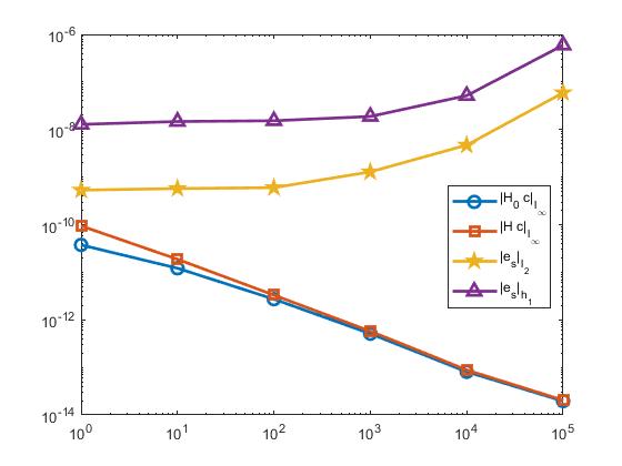
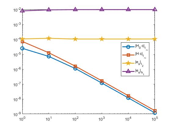
Figure 3: The accuracies of the solutions $|e_{s}|_{l_{2}},|e_{s}|_{h}$ and the smoothness $|H_{0}c|_{l_{\infty}},|Hc|_{l_{\infty}}$ based on testing functions $u^{s5}$(left) and $u^{s8}$(right) with $\alpha=\gamma=1$ for various $\beta$

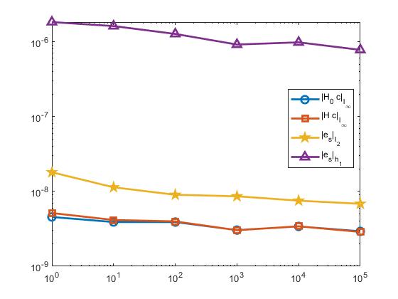
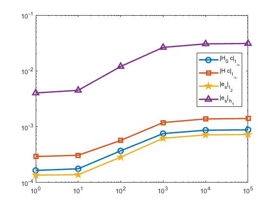
Figure 4: The accuracies of the solutions $|e_{s}|_{l_{2}},|e_{s}|_{h}$ and the smoothness $|H_{0}c|_{l_{\infty}},|Hc|_{l_{\infty}}$ based on testing functions $u^{s5}$(left) and $u^{s8}$(right) with $\beta=\gamma=1$ for various $\alpha$

6 Numerical results for the Poisson Equation

We shall present computational results for 2D Poisson equation and 3D Poisson equations separately in the following two subsections. In each section, we first present the computational results from the spline based collocation method to demonstrate the accuracy the method can achieve. Then we present a comparison of our collocation method with the numerical method proposed in [2] which uses multivariate splines to find the weak solution like finite element method. For convenience, we shall call our spline based collocation method the LL method and the numerical method in [2] the AWL method.

6.1 Numerical examples for 2D Poisson equations

We have used various triangulations over various bounded domains to experiment the performance of our Algorithm  1 in [15] and tested many solutions to the Poisson equation to see the accuracy that the LL method can do. For convenience, we shall only present a few of the computational results based on the domains in Figure 1. The following is a list of 10 testing functions (8 smooth solutions and 2 not very smooth)

$$u^{s1} = e^{\frac{(x^{2}+y^{2})}{2}},$$

$$u^{s2} = \cos(xy)+\cos(\pi(x^{2}+y^{2})),$$

$$u^{s3} = \frac{1}{1+x^{2}+y^{2}},$$

$$u^{s4} = \sin(\pi(x^{2}+y^{2}))+1,$$

$$u^{s5} = \sin(3\pi x)\sin(3\pi y),$$

$$u^{s6} = \arctan(x^{2}-y^{2}),$$

$$u^{s7} = -\cos(x)\cos(y)e^{-(x-\pi)^{2}-(y-\pi)^{2}}$$

$$u^{s8} = \tanh(20y-20x^{2})-\tanh(20x-20y^{2}),$$

$$u^{ns1} = |x^{2}+y^{2}|^{0.8}\hbox{ and }$$

$$u^{ns2} = (xe^{1-|x|}-x)(ye^{1-|y|}-y).$$

Note that the testing function in $u^{s8}$ is notoriously difficult to solve. One has to use a good adaptive triangulation method (cf. [9]). The rooted mean square (RMS) of $u-u_{s}$ and $\nabla(u-u_{s})$ of approximate spline solution $u_{s}$ against the exact solution $u$ are given in Table 4. These errors are computed based on $1001\times 1001$ equally-spaced points of the bounding box of a domain in in Figure 1 which fell inside the domain. We chose collocation points to create $M\times m$ matrix $K$, where $m$ is the number of Bernstein basis functions (the dimension of spline space $S^{-1}_{D}(\triangle)$) and Algorithm 1 is used to find the numerical solutions.

	Moon		Flower with a hole		Star with 2 holes		Circle with 3 holes
Solution	$u-u_{s}$	$\nabla(u-u_{s})$	$u-u_{s}$	$\nabla(u-u_{s})$	$u-u_{s}$	$\nabla(u-u_{s})$	$u-u_{s}$	$\nabla(u-u_{s})$
$u^{s1}$	6.95e-11	4.15e-10	1.23e-11	1.54e-10	1.67e-12	6.57e-11	1.63e-11	1.68e-10
$u^{s2}$	3.53e-10	4.81e-09	1.83e-11	8.79e-10	2.46e-12	9.77e-11	2.65e-11	2.55e-10
$u^{s3}$	2.58e-11	1.81e-10	6.96e-12	9.48e-11	1.48e-12	5.66e-11	8.03e-12	8.73e-11
$u^{s4}$	2.53e-10	3.57e-09	2.19e-11	6.80e-10	1.45e-12	8.41e-11	1.92e-11	2.00e-10
$u^{s5}$	6.16e-08	1.44e-06	7.73e-09	2.57e-07	3.02e-10	1.36e-08	5.33e-10	1.87e-08
$u^{s6}$	1.75e-11	2.86e-10	3.23e-12	8.71e-11	2.97e-13	7.23e-12	7.51e-12	7.85e-11
$u^{s7}$	3.07e-12	2.27e-11	1.15e-12	1.51e-11	2.81e-13	6.69e-12	1.10e-12	1.28e-11
$u^{s8}$	1.06e-03	9.32e-02	8.65e-04	8.38e-02	4.84e-05	3.36e-03	5.21e-04	2.09e-02
$u^{ns1}$	7.31e-10	3.68e-08	5.18e-06	4.94e-04	2.62e-06	3.89e-04	1.80e-05	3.22e-04
$u^{ns2}$	3.16e-04	2.61e-03	7.39e-05	1.51e-03	2.75e-05	9.76e-04	1.91e-05	6.25e-04

Table 4: The RMS of errors $u-u_{s}$ and $\nabla u-\nabla u_{s}$ for Poisson equations for four domains showed in Figure 1 when $r=2$ and $D=8$.

From Table 4, we can see that the performance of our method is excellent. Next let us compare with the numerical method in [2] for the same degree, the same smoothness, and the same triangulation. The comparison results are shown in Table 5. One can see that both methods perform very well. Our method can achieve a better accuracy due to the reason the more number of collocation points is used than the dimension of spline space $S^{-1}_{D}(\triangle)$.

	Moon		Flower with a hole		Star with 2 holes		Circle with 3 holes
Sol’n	AWL	LL	AWL	LL	AWL	LL	AWL	LL
$u^{s1}$	1.51e-07	6.95e-11	1.14e-07	1.23e-11	2.08e-07	1.67e-12	5.22e-08	1.63e-11
$u^{s2}$	1.33e-07	3.53e-10	3.79e-07	1.83e-11	8.93e-07	2.46e-12	2.35e-08	2.65e-11
$u^{s3}$	4.94e-08	2.58e-11	8.07e-08	6.96e-12	1.44e-07	1.48e-12	1.62e-08	8.03e-12
$u^{s4}$	5.77e-07	2.53e-10	3.89e-07	2.19e-11	4.51e-07	1.45e-12	2.02e-07	1.92e-11
$u^{s5}$	1.58e-06	6.16e-08	1.43e-06	7.73e-09	1.67e-06	3.02e-10	2.65e-07	5.33e-10
$u^{s6}$	5.00e-07	1.75e-11	1.44e-07	3.23e-12	4.03e-07	2.97e-13	9.47e-08	7.51e-12
$u^{s7}$	1.99e-08	3.07e-12	2.20e-08	1.15e-12	3.30e-08	2.81e-13	4.97e-09	1.10e-12
$u^{s8}$	1.31e-03	1.06e-03	1.19e-03	8.65e-04	1.49e-04	4.84e-05	7.96e-04	5.21e-04
$u^{ns1}$	1.50e-07	7.31e-10	2.39e-04	5.18e-06	2.26e-05	2.62e-06	1.43e-05	1.80e-05
$u^{ns2}$	1.38e-03	3.16e-04	4.55e-04	7.39e-05	9.87e-05	2.75e-05	8.57e-05	1.91e-05

Table 5: RMSE of spline solutions for the Poisson equation over the four domains in Figure 1 when $r=2$ and $D=8$ for both the AWL method and the LL method.

Finally, we summarize the computational times for both methods in Table 6. One can see the LL method can be more efficient if the collocation matrices are already generated. The LL method can be useful for time dependent PDE such as the heat equation. We only need to generate the collocation matrix once and use it repeatedly for many time step iterations.

Domain	Number of	Number of	Average time	Average time for
	vertices	triangles	for AWL method	LL method (part 2)
Moon	325	531	9.61e-01	6.28e-01
Flower with a hole	297	494	8.05e-01	5.39e-01
Star with 2 holes	231	366	5.53e-01	3.97e-01
Circle with 3 holes	525	895	1.44e+00	9.74e-01

Table 6: The number of vertices, triangles and the averaged time for solving the 2D Poisson equation for each domain in Figure 1.

6.2 Numerical results for the 3D Poisson equation

We have used our collocation method to solve the 3D Poisson equation and the tested 10 smooth and non-smooth solution over various domains. For convenience, we only show a few computational results to demonstrate that our collocation method works very well. More detail can be found in [15]. Our testing solutions are as follows:

$$u^{3ds1} = \sin(2x+2y)\tanh(\frac{xz}{2})$$

$$u^{3ds2} = e^{\frac{x^{2}+y^{2}+z^{2}}{2}}$$

$$u^{3ds3} = \cos(xyz)+\cos(\pi(x^{2}+y^{2}+z^{2}))$$

$$u^{3ds4} = \frac{1}{1+x^{2}+y^{2}+z^{2}}$$

$$u^{3ds5} = \sin(\pi(x^{2}+y^{2}+z^{2}))+1$$

$$u^{3ds6} = 10e^{-x^{2}-y^{2}-z^{2}}$$

$$u^{3ds7} = \sin(2\pi x)\sin(2\pi y)\sin(2\pi z)$$

$$u^{3ds8} = z\tanh((-\sin(x)+y^{2}))$$

$$u^{3dns1} = |x^{2}+y^{2}+z^{2}|^{0.8}$$

$$u^{3dns2} = (xe^{1-|x|}-x)(ye^{1-|y|}-y)(ze^{1-|z|}-z).$$

The rooted mean squared errors of approximate spline solutions against the exact solution are computed based on $501\times 501\times 501$ equally-spaced points of the bounding box of a domain shown in Figure 2 which fall into the domain.

	Letter C		Letter S		Torus		Human head
Solution	$u-u_{s}$	$\nabla(u-u_{s})$	$u-u_{s}$	$\nabla(u-u_{s})$	$u-u_{s}$	$\nabla(u-u_{s})$	$u-u_{s}$	$\nabla(u-u_{s})$
$u^{3ds1}$	2.31e-11	2.52e-10	3.01e-12	4.58e-11	7.87e-11	1.40e-09	4.12e-10	5.02e-09
$u^{3ds2}$	5.47e-10	4.86e-09	7.53e-12	7.31e-11	4.52e-09	3.24e-08	1.66e-08	1.29e-07
$u^{3ds3}$	5.49e-07	8.40e-06	8.87e-08	7.80e-07	3.32e-09	3.21e-08	9.96e-06	1.65e-04
$u^{3ds4}$	4.83e-09	5.09e-08	4.29e-09	3.85e-08	2.16e-09	1.61e-08	1.13e-08	2.21e-07
$u^{3ds5}$	6.49e-07	1.67e-05	1.17e-07	9.47e-07	7.07e-09	5.78e-08	3.62e-06	5.88e-05
$u^{3ds6}$	3.52e-09	3.99e-08	8.39e-10	6.53e-09	2.03e-08	1.72e-07	6.69e-08	6.90e-07
$u^{3ds7}$	9.14e-06	8.63e-05	3.20e-06	2.44e-05	1.40e-07	4.75e-06	4.31e-05	8.24e-04
$u^{3ds8}$	2.05e-08	2.79e-07	3.30e-09	3.35e-08	1.76e-10	2.98e-09	1.90e-08	3.94e-07
$u^{3dns1}$	8.80e-06	4.66e-04	3.17e-05	1.14e-03	2.23e-09	1.80e-08	8.28e-06	2.18e-03
$u^{3dns2}$	8.39e-05	1.20e-03	4.30e-05	4.65e-04	1.20e-04	2.49e-03	8.90e-04	5.18e-02

Table 7: RMS of error vectors $u-u_{s}$ and $\nabla u-\nabla u_{s}$ for the 3D Poisson equation over the four domains in Figure 2 based on trivariate spline functions of smoothness $r=1$ and degree $D=9$

We choose collocation points to create $M\times m$ matrix $K$, where $m$ is the dimension of spline space $S^{-1}_{D}(\triangle)$ and apply Algorithm 1 to find the numerical solutions. We tested 10 functions over the domains in Figure 2. Their root mean square errors are presented in Table 7. We also compare the AWL method with LL method for the numerical solution of the 3D Poisson equation. See numerical results in Table 8 which show that the LL method is more accurate than the AWL method when the solutions are smooth and is similar to the AWL method when the solutions are not very smooth.

	Torus				Human head
	AWL		LL		AWL		LL
Solution	$u-u_{s}$	$\nabla(u-u_{s})$	$u-u_{s}$	$\nabla(u-u_{s})$	$u-u_{s}$	$\nabla(u-u_{s})$	$u-u_{s}$	$\nabla(u-u_{s})$
$u^{3ds1}$	3.55e-09	5.74e-07	1.79e-10	2.04e-09	2.83e-09	7.56e-07	5.83e-12	6.45e-11
$u^{3ds2}$	2.92e-08	1.98e-06	1.14e-08	8.50e-08	5.21e-07	2.72e-06	3.45e-10	2.95e-09
$u^{3ds3}$	1.07e-07	8.90e-06	5.34e-09	3.31e-08	6.44e-08	1.21e-05	7.26e-10	8.21e-09
$u^{3ds4}$	1.88e-08	1.46e-06	3.57e-09	2.29e-08	1.83e-08	2.72e-06	2.68e-10	2.76e-09
$u^{3ds5}$	8.25e-08	5.50e-06	1.33e-08	8.95e-08	6.09e-08	8.43e-06	9.75e-10	5.78e-09
$u^{3ds6}$	2.50e-07	1.80e-05	3.39e-08	1.90e-07	1.31e-07	1.35e-05	2.35e-09	2.47e-08
$u^{3ds7}$	8.07e-08	5.83e-06	1.01e-07	2.34e-06	1.88e-08	2.72e-06	4.19e-08	5.21e-07
$u^{3ds8}$	8.16e-09	7.24e-07	6.42e-10	4.32e-09	8.16e-09	3.41e-07	2.69e-11	1.66e-10
$u^{3dns1}$	3.92e-08	2.67e-06	5.07e-09	3.22e-08	3.63e-08	2.67e-06	3.82e-06	6.23e-04
$u^{3dns2}$	6.30e-04	2.29e-03	1.09e-04	1.58e-03	3.42e-04	2.49e-03	2.30e-04	4.84e-03

Table 8: The RMSE of spline solutions for the 3D Poisson equation over the two domains in Figure 2 based on trivariate spline functions of smoothness $r=1$ and degree $D=9$ for the AWL method and LL method.

7 Numerical Results for General Second Order Elliptic PDE

We shall present computational results for 2D and 3D general second order PDEs separately in the following two subsections. In each section, we first present the computational results from the spline based collocation method to demonstrate the accuracy the method can achieve. Then we present a comparison of our collocation method with the numerical method based on [12]. For convenience, we shall call our spline based collocation method the LL method and the numerical method in [12] the LW method.

7.1 Numerical examples for 2D general second order equations

We have used the same triangulations over various bounded domains as shown in Figure 1 and tested the same solutions which we used for the Poisson equation for the general second order equation to see the accuracy that the LL method can have. The root mean squared error(RMSE) $u-u_{s}$ and $\nabla u-\nabla u_{s}$ of approximate spline solutions $u_{s},\nabla u_{s}$ against the exact solutions $u,\nabla u$ are given in Tables in this section. The RMSE are computed based on $1001\times 1001$ equally-spaced points of the bounding box of a domain in Figure 1 which fell inside the domain. We chose additional collocation points to create $M\times m$ matrix $\mathcal{K}$, where $m,M$ are the dimension of spline space $S^{-1}_{D}(\triangle)$ and $S^{-1}_{D^{\prime}}(\triangle)$, respectively.

7.1.1 2D general second order equations with smooth coefficients

Example 1

We first tested our computational method to solve the 2nd order elliptic equation with smooth PDE coefficients: $a_{11}=x^{2}+y^{2},a_{12}=\cos(xy),a_{21}=e^{xy},a_{22}=x^{3}+y^{2}-\sin(x^{2}+y^{2}),b_{1}=3\cos(x)y^{2},b_{2}=e^{-x^{2}-y^{2}},c=0$. Our testing functions are 2 non-smooth solutions $u^{ns1},u^{ns2}$, and 8 smooth solutions $u^{s1}$ — $u^{s8}$ given in the previous section. The RMS of error vectors $u-u_{s}$ and $\nabla(u-u_{s})$ over the four domains in Figure 1 is presented in Table 9. The numerical results show that the LL method works very well.

	Moon		Flower with a hole		Star with 2 holes		Circle with 3 holes
Solution	$u-u_{s}$	$\nabla(u-u_{s})$	$u-u_{s}$	$\nabla(u-u_{s})$	$u-u_{s}$	$\nabla(u-u_{s})$	$u-u_{s}$	$\nabla(u-u_{s})$
$u^{s1}$	3.11e-10	6.25e-09	1.63e-10	5.62e-09	4.96e-11	1.93e-09	4.05e-10	1.06e-08
$u^{s2}$	7.86e-10	1.51e-08	6.95e-10	2.98e-08	1.33e-10	4.04e-09	3.27e-10	1.18e-08
$u^{s3}$	2.90e-10	4.12e-09	1.72e-10	4.77e-09	4.07e-11	1.60e-09	1.78e-10	6.25e-09
$u^{s4}$	4.79e-10	1.51e-08	4.38e-10	1.59e-08	5.33e-11	2.41e-09	5.05e-10	1.26e-08
$u^{s5}$	5.35e-08	3.40e-06	5.90e-08	2.58e-06	8.84e-10	6.81e-08	3.04e-09	1.93e-07
$u^{s6}$	1.24e-10	2.52e-09	4.19e-11	1.83e-09	1.11e-11	3.56e-10	1.29e-10	2.44e-09
$u^{s7}$	2.65e-11	4.32e-10	3.02e-11	1.40e-09	7.06e-12	3.07e-10	5.81e-11	1.23e-09
$u^{s8}$	9.04e-03	2.61e-01	9.81e-03	3.63e-01	2.50e-04	1.35e-02	2.28e-03	1.29e-01
$u^{ns1}$	8.26e-10	6.54e-08	4.62e-06	6.85e-04	1.69e-06	4.87e-04	5.78e-05	6.17e-03
$u^{ns2}$	2.01e-04	3.24e-03	2.97e-04	6.88e-03	1.27e-04	5.80e-03	7.33e-05	2.84e-03

Table 9: RMSE of spline solutions for general second order elliptic equations with smooth coefficients over the four domains in Figure 1 when $r=2$ and $D=8$.

7.1.2 2D general second order equations with non-smooth coefficients

Example 2

In [19], the researchers experimented their numerical methods for the second order PDE as follows:

$$\sum^{2}_{i,j=1}(1+\delta_{ij})\frac{x_{i}}{|x_{i}|}\frac{x_{j}}{|x_{j}|}u_{x_{i}x_{j}}=f~{}~{}\hbox{ in }\Omega,\quad u=0~{}on~{}\partial\Omega,$$

where $\Omega=(-1,1)^{2}$ and the solution $u$ is $u(x,y)=(xe^{1-|x|}-x)(ye^{1-|y|}-y)$ which is one of our testing functions. It is easy to see those coefficients satisfy the Cordes condition

$$\frac{\sum_{i,j=1}^{d}(a_{i,j})^{2}}{(\sum_{i=1}^{2}a_{ii})^{2}}=\frac{2^{2}+1+1+2^{2}}{(2+2)^{2}}=\frac{10}{16}\leq\frac{1}{2-1+\epsilon}$$

when $\epsilon=\frac{3}{5}$. This equation was also numerically experimented in [12] and [20].

Let us test our method on this 2nd order elliptic equation with non-smooth coefficients for the 2 non-smooth solutions $u^{ns1},u^{ns2}$, and 8 smooth solutions $u^{s1}-u^{s8}$ over the four domains used in the previous section. We use bivariate splines of degree $D=8$ and smoothness $r=2$ for the experiment. And the RMSE of the solutions for the four domains in Figure 1 are reported in Table 10. It is clear to see that our method works very well.

	Moon		Flower with a hole		Star with 2 holes		Circle with 3 holes
Solution	$u-u_{s}$	$\nabla(u-u_{s})$	$u-u_{s}$	$\nabla(u-u_{s})$	$u-u_{s}$	$\nabla(u-u_{s})$	$u-u_{s}$	$\nabla(u-u_{s})$
$u^{s1}$	1.36e-10	1.24e-09	8.79e-11	1.34e-09	2.85e-11	3.73e-09	1.03e-11	1.14e-10
$u^{s2}$	1.95e-10	2.59e-09	1.16e-10	2.15e-09	2.97e-11	2.02e-09	1.66e-11	1.73e-10
$u^{s3}$	5.20e-11	4.91e-10	5.21e-11	8.99e-10	1.52e-11	1.07e-09	5.20e-12	5.85e-11
$u^{s4}$	2.16e-10	2.46e-09	9.81e-11	1.83e-09	2.68e-11	2.06e-09	1.61e-11	1.82e-10
$u^{s5}$	6.26e-08	1.27e-06	1.33e-08	3.24e-07	5.04e-10	2.02e-08	7.58e-10	1.64e-08
$u^{s6}$	3.92e-11	4.46e-10	1.61e-11	2.63e-10	4.77e-12	2.07e-10	3.25e-12	3.81e-11
$u^{s7}$	3.43e-12	3.26e-11	1.26e-11	2.00e-10	2.81e-12	2.45e-10	1.22e-12	1.20e-11
$u^{s8}$	1.44e-03	9.95e-02	2.86e-03	1.20e-01	1.11e-04	4.07e-03	1.87e-04	1.67e-02
$u^{ns1}$	2.00e-09	5.73e-08	1.57e-04	3.88e-03	2.59e-04	4.30e-03	1.50e-05	5.31e-04
$u^{ns2}$	1.60e-03	1.62e-02	1.03e-03	1.73e-02	8.84e-04	1.61e-02	2.56e-04	4.03e-03

Table 10: RMSE $u-u_{s}$ and $\nabla u-\nabla u_{s}$ for the general elliptic equation with the non-smooth coefficients in Example 2 over the four domains in Figure 1 when $r=2$ and $D=8$.

Example 3

The second example in the paper [19] is another second order PDE:

$$\sum^{2}_{i,j=1}(\delta_{ij}+\frac{x_{i}x_{j}}{|x|^{2}})u_{x_{i}x_{j}}=f~{}~{}in~{}\Omega,\quad u=0~{}on~{}\partial\Omega,$$

where $\Omega=(-1,1)^{2}$ and the solution $u$ is $u(x,y)=|x^{2}+y^{2}|^{\frac{\alpha}{2}}$ which is on the list of our testing functions. Then those coefficients satisfy the Cordes condition when $\epsilon=\frac{4}{5}$.

	Moon		Flower with a hole		Star with 2 holes		Circle with 3 holes
Solution	$u-u_{s}$	$\nabla(u-u_{s})$	$u-u_{s}$	$\nabla(u-u_{s})$	$u-u_{s}$	$\nabla(u-u_{s})$	$u-u_{s}$	$\nabla(u-u_{s})$
$u^{s1}$	2.20e-11	1.81e-10	2.26e-11	4.32e-10	1.04e-11	2.38e-09	6.64e-12	7.61e-11
$u^{s2}$	1.64e-10	2.67e-09	2.52e-11	1.03e-09	1.50e-11	2.49e-09	7.34e-12	1.04e-10
$u^{s3}$	1.41e-11	1.08e-10	1.72e-11	3.33e-10	9.64e-12	1.80e-09	4.03e-12	4.67e-11
$u^{s4}$	1.75e-10	2.14e-09	4.16e-11	9.44e-10	1.80e-11	3.92e-09	9.03e-12	1.22e-10
$u^{s5}$	3.71e-08	8.57e-07	6.13e-09	2.01e-07	3.78e-10	1.58e-08	5.95e-10	1.35e-08
$u^{s6}$	5.70e-12	2.31e-10	6.56e-12	1.31e-10	1.33e-12	2.73e-10	1.77e-12	2.38e-11
$u^{s7}$	1.42e-12	1.21e-11	3.23e-12	6.56e-11	1.24e-12	2.63e-10	4.61e-13	5.59e-12
$u^{s8}$	1.15e-03	8.63e-02	2.11e-03	8.77e-02	5.51e-05	3.41e-03	1.46e-04	1.61e-02
$u^{ns1}$	3.58e-10	4.08e-08	1.31e-04	3.45e-03	2.11e-04	4.12e-03	3.26e-05	1.01e-03
$u^{ns2}$	1.95e-04	1.97e-03	5.78e-05	1.35e-03	2.73e-05	9.06e-04	1.60e-05	5.25e-04

Table 11: The RMS of vectors $u-u_{s},\nabla u-\nabla u_{s}$ for general elliptic equations with non-smooth coefficients in Example 3 over the four domains when $r=2$ and $D=8$.

Similar to Example 2, we use the LL method to solve the PDE above using the 10 testing functions based on bivariate splines of degree $D=8$ and smoothness $r=2$. See Table 11 for the RMS of error vectors.

7.2 Comparison with Numerical Method in [12]

We first compare our LL method with the LW method in [12] when numerically solving three PDEs given in Examples 1, 2, and 3. The RMSEs from the two methods will be reported in Table 12. For simplicity, we only present the numerical results from the two computational methods over the Circle with 3 holes in Table 12. We get the similar results for other 2D domains in Figure 1. From Table 12, we see that the LL method produces more accurate results.

	PDE in Example 1		PDE in Example 2		PDE in Example 3
Method	LW	LL	LW	LL	LW	LL
$u^{s1}$	2.01e-09	1.49e-10	2.15e-06	1.03e-11	7.47e-09	6.64e-12
$u^{s2}$	2.22e-08	4.31e-11	2.97e-05	1.66e-11	3.86e-08	7.34e-12
$u^{s3}$	1.70e-09	8.85e-11	4.96e-06	5.20e-12	2.97e-09	4.03e-12
$u^{s4}$	2.29e-08	2.12e-10	6.13e-05	1.61e-11	7.66e-08	9.03e-12
$u^{s5}$	8.24e-08	3.37e-09	4.19e-04	7.58e-10	1.20e-06	5.95e-10
$u^{s6}$	2.63e-09	3.72e-11	4.11e-06	3.25e-12	3.15e-09	1.77e-12
$u^{s7}$	3.06e-14	1.05e-11	2.10e-11	1.22e-12	2.66e-14	4.61e-13
$u^{s8}$	8.50e-04	2.26e-03	2.54e-03	1.87e-04	1.78e-04	1.46e-04
$u^{ns1}$	1.35e-05	4.83e-05	3.57e-05	1.50e-05	1.52e-05	3.26e-05
$u^{ns2}$	2.45e-04	4.56e-05	1.60e-04	2.56e-04	5.92e-05	1.60e-05

Table 12: The RMSE of spline solutions for general elliptic equations in Example 1, PDE with non-smooth coefficients in Example 2 and in Example 3 over the Circle with 3 holes when $r=2$ and $D=8$ for the LW method and the LL method, respectively.

Next Table 13 shows the averaged computational time for the LL method is shorter than the LW method.

Domain	Number of	Number of	Average time	Average time
	vertices	triangles	for LW method	for Part 2 of LL method
Flower with a hole	297	494	1.3236e+02	3.521e-01
Circle with 3 holes	525	895	4.4387e+03	8.313e-01

Table 13: The number of vertices, triangles and the averaged time in seconds for solving 2D general second order equations over the four domains in Figure 1 by the LW and LL methods.

Combining the computational results in Table 13 and computational times in Table 12, we conclude that the LL method is more effective and efficient than the LW method.

8 The Rate of Convergence of the LL method

Finally, we discuss the rate of convergence of the LL method. First in Example 4, we conduct an experiment on the rate of convergence based on numerical solutions of the 2D general elliptic PDEs in Example 1 over $[0,1]^{2}$. The rate of convergence with respect to the size $h=|\triangle|$ of triangulation $\triangle$ is shown in Figure 5. In addition we show the rate of convergence with respect to the DOF which is presented in Figure 6. Similarly in Example 5, we first present the rate of convergence based on the numerical solutions of the 3D general elliptic PDE with smooth coefficients with respect to the size $h$ of triangulations in Figure 7 and then we present the rate of convergence with respect to the DOFs.

Example 4

We numerically solved the general elliptic equations in Example 1 with $D=8,r=2$ for testing functions $u^{s2}$ and $u^{s4}$ on different levels of the refinement to demonstrate the convergence behavior. The $L^{2},H^{1}$ error vectors $u-u_{s}$ based on $1001^{2}$ equally-spaced points over $[0,1]^{2}$ with respect to the size $h=|\triangle|$ are reported in Figure 5. We can see that the rate of convergence is about $O(h^{7})$. According to Theorem 6, the $\|u-u_{s}\|_{2}\leq Ch^{2}\epsilon$. This shows that the numerical computation agrees with and even better than the theory we have.

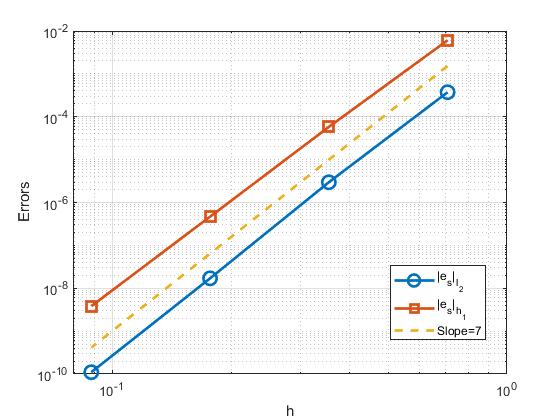
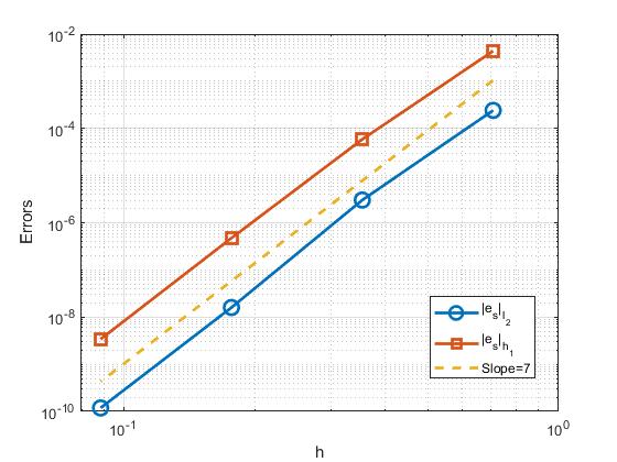
Figure 5: The RMSE in $L^{2}$ and $H^{1}$ norm of $u-u_{s}$ for testing functions $u^{s2}$(left) and $u^{s4}$(right) versus the size $h$ of triangulation with $D=8,r=2$ where $e_{s}:=u-u_{s}$

Next convergence results are shown in Figure 6 based on the DOF(=the number of triangles $\times\dfrac{(D+1)(D+2)}{2}$). The RMSEs between the numerical solution and exact solutions are asymptotically proportional to $(\text{DOF})^{-3.5}$. That is, the asymptotic rate is $(\text{DOF})^{-1/(d+1)}$, where $d=2$. See the next example when $d=3$.

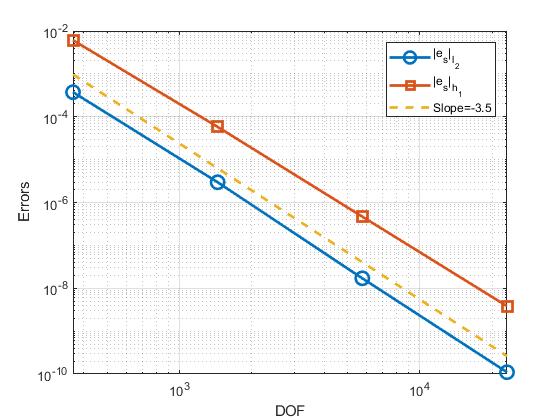
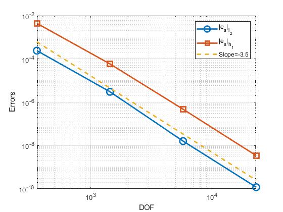
Figure 6: The RMSE in $L^{2}$ and $H^{1}$ norm of $u-u_{s}$ for testing functions $u^{s2}$(left) and $u^{s4}$(right) versus the DOFs with $D=8,r=2$ where $e_{s}:=u-u_{s}$

Example 5

We tested a 2nd order elliptic equation (2) with smooth PDE coefficients $a_{11}=x^{2}+y^{2},a^{22}=\cos(xy-z),a^{33}=\exp(\frac{1}{x^{2}+y^{2}+z^{2}+1}),a^{12}+a^{21}=x^{2}-y^{2}-z,a^{23}+a^{32}=\cos(xy-z)\sin(x-y),a^{13}+a^{31}=\frac{1}{y^{2}+z^{2}+1},b_{1}=0,b_{2}=-1,b_{3}=\tan^{-1}(x^{3}-y^{2}+\cos(z)),c=x+y+z$, where $a^{12}=a^{21},a^{32}=a^{23}$ and $a^{13}=a^{31}.$ The testing functions are the 2 smooth solutions $u^{3ds3},u^{3ds5}$ over the standard cube $[0,1]^{3}$. The $L^{2},H^{1}$ error vectors $u-u_{s}$ based on $501^{3}$ equally-spaced points over $[0,1]^{3}$ are reported in Figure 7. The errors between the numerical solution and exact solutions are asymptotically proportional to $\mathcal{O}(h^{7})$. We can see that the rate of convergence agrees with our theory for these smooth testing functions. Therefore, we conclude that the LL methods work very well.

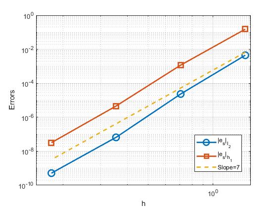
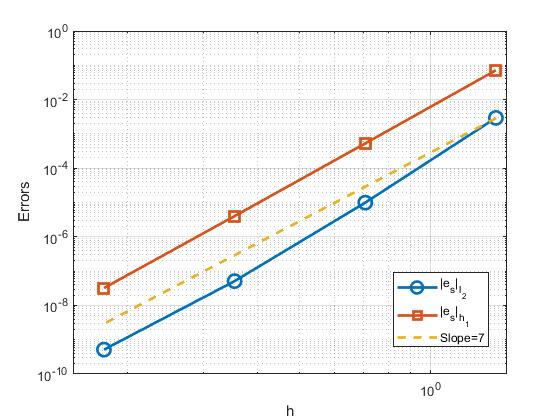
Figure 7: The RMSE in $L^{2}$ and $H^{1}$ norm of $u-u_{s}$ with $D=9,r=1$ for testing functions $u^{3ds3}\text{(left)}$ and $u^{3ds5}\text{(right)}$ versus the mesh size $h$

In addition, we show the rate of convergence with respect to the DOFs in Figure 8 based on the DOF(=the number of triangles $\times\dfrac{(D+1)(D+2)(D+3)}{6}$).

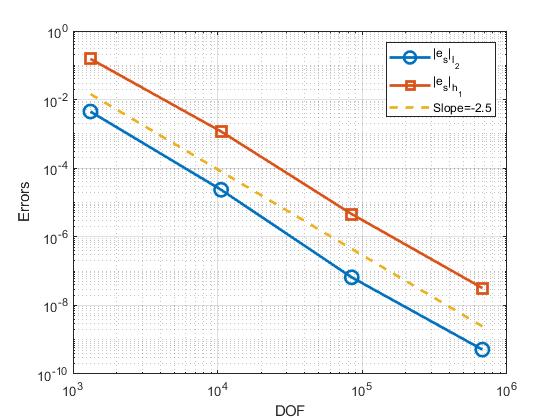
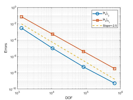
Figure 8: The RMSE in $L^{2}$ and $H^{1}$ norm of $u-u_{s}$ with $D=9,r=1$ for testing functions $u^{3ds3}\text{(left)}$ and $u^{3ds5}\text{(right)}$ versus the DOFs

9 Appendix: Convergence of Algorithm 1

In this section, we first explain Algorithm 1 which is used to solve the minimization problem (17). In fact, Algorithm 1 is derived based on the solution to the following minimization

$$\min_{\bf c}J(c)=\frac{1}{2}(\alpha\|B{\bf c}-{\bf g}\|^{2}+\beta\|H_{r}{\bf c}\|^{2}+\gamma\|H_{0}{\bf c}\|^{2})\quad\text{subject to }-K{\bf c}={\bf f},$$ (38)

where $B,{\bf g}$ are associated with the boundary condition, $H_{r}$ is associated with the smoothness condition $\alpha>0,\beta>0$ are fixed parameters. Let us give a reason why we use (38) to replace (17). By Lemma 2, we know spline functions can approximate the solution of the PDE very well when the solution $u$ is in $H^{3}(\Omega)$. When the size $|\triangle|$ is small enough, for the quasi-interpolatory spline $S_{u}$ can approximate $u$ such that $\|\Delta(u-S_{u})\|_{L^{2}(\Omega)}\leq\epsilon_{1}.$ That is, the feasible set of (17) is not empty. Thus, two minimization problems (17) and (38) are closely related to each other. Even though there is not ${\bf c}$ satisfying $-K{\bf c}={\bf f}$ exactly, a numerical computation in a computer will give a nearby solution ${\bf c}$ such that $\|K{\bf c}+{\bf f}\|\leq\epsilon_{1}$. We thus seek a spline solution $u_{s}$ satisfying (38).

We use the similar technique in [1] and [2]. For convenience, we first consider the problem

$$\min_{\bf c}J(c)=\frac{1}{2}(\alpha\|B{\bf z}-{\bf g}\|^{2}+\beta\|H{\bf z}\|^{2})\quad\text{subject to }-K{\bf z}={\bf f},$$ (39)

where $B,{\bf g}$ are from the boundary condition, $H$ is from the smoothness condition. By the theory of Lagrange multipliers, letting

$$\mathcal{U}(z,\lambda)=\frac{1}{2}(\alpha z^{\intercal}B^{\intercal}Bz-\alpha z^{\intercal}B^{\intercal}G-\alpha G^{\intercal}Bz+\alpha G^{\intercal}G+\beta z^{\intercal}H^{\intercal}Hz)+\lambda^{\intercal}(K{\bf z}+{\bf f}),$$

there exist $\lambda$ such that

$$\frac{\partial\mathcal{U}}{\partial z}=\alpha B^{\intercal}Bz-\alpha B^{\intercal}G+\beta H^{\intercal}Hz+K^{\intercal}\lambda=0$$ (40)

$$\frac{\partial\mathcal{U}}{\partial\lambda}=K{\bf z}+{\bf f}=0$$ (41)

We can rewrite above linear equations as follow:

$$\begin{bmatrix}K^{\intercal}&\alpha B^{\intercal}B+\beta H^{\intercal}H\\ O&K\end{bmatrix}\begin{bmatrix}\lambda\\ z\end{bmatrix}=\begin{bmatrix}\alpha B^{\intercal}G\\ -{\bf f}\end{bmatrix}$$ (42)

To solve (42), we consider the following sequence of problems for a fixed $\epsilon>0$:

$$\begin{bmatrix}K^{\intercal}&\alpha B^{\intercal}B+\beta H^{\intercal}H\\ -\epsilon I&K\end{bmatrix}\begin{bmatrix}\lambda^{(k+1)}\\ z^{(k+1)}\end{bmatrix}=\begin{bmatrix}\alpha B^{\intercal}G\\ -{\bf f}-\epsilon\lambda^{(k)}\end{bmatrix}$$ (43)

for $k=0,1,\cdots,$ with an initial guess $\lambda^{(0)}=0$. Note that (43) reads

$$(\alpha B^{\intercal}B+\beta H^{\intercal}H)z^{(k+1)}+K^{\intercal}\lambda^{(k+1)}=\alpha B^{\intercal}G$$

$$Kz^{(k+1)}-\epsilon\lambda^{(k+1)}=-{\bf f}-\epsilon\lambda^{(k)}$$

Multiplying on the both sides of the second equation in (43) by $K^{\intercal}$, we get

$$K^{\intercal}Kz^{(k+1)}-\epsilon K^{\intercal}\lambda^{(k+1)}=-K^{\intercal}{\bf f}-\epsilon K^{\intercal}\lambda^{(k)}$$

or

$$K^{\intercal}\lambda^{(k+1)}=\frac{1}{\epsilon}K^{\intercal}Kz^{(k+1)}-\frac{1}{\epsilon}K^{\intercal}{\bf f}+K^{\intercal}\lambda^{(k)}$$

and substitute it into the first equation in (43) to get

$$(\alpha B^{\intercal}B+\beta H^{\intercal}H)z^{(k+1)}+\frac{1}{\epsilon}K^{\intercal}Kz^{(k+1)}-\frac{1}{\epsilon}K^{\intercal}{\bf f}+K^{\intercal}\lambda^{(k)}=\alpha B^{\intercal}G.$$

Simplifying the above equation leads to

$$(\alpha B^{\intercal}B+\beta H^{\intercal}H+\frac{1}{\epsilon}K^{\intercal}K)z^{(k+1)}=\alpha B^{\intercal}G+\frac{1}{\epsilon}K^{\intercal}{\bf f}-K^{\intercal}\lambda^{(k)}$$ (44)

It follows that

$$z^{(1)}=(\alpha B^{\intercal}B+\beta H^{\intercal}H+\frac{1}{\epsilon}K^{\intercal}K)^{-1}(\alpha B^{\intercal}G+\frac{1}{\epsilon}K^{\intercal}{\bf f}-K^{\intercal}\lambda^{(0)})$$ (45)

Using the first equation in (43),i.e., $(\alpha B^{\intercal}B+\beta H^{\intercal}H)z^{(k+1)}=\alpha B^{\intercal}G-K^{\intercal}\lambda^{(k+1)}$ to replace $\alpha B^{\intercal}G$ in (44), we have

$$(\alpha B^{\intercal}B+\beta H^{\intercal}H+\frac{1}{\epsilon}K^{\intercal}K)z^{(k+1)}=(\alpha B^{\intercal}B+\beta H^{\intercal}H)z^{(k)}+\frac{1}{\epsilon}K^{\intercal}{\bf f}.$$ (46)

We get the minimizer using (45) and (46). These lead to Algorithm 1.

Next we show the convergence of the above iterative algorithm. Since the minimization problem (17) is convex over a convex feasible set, we know that the minimization has a unique solution. We may assume that the linear system from Lagrange multiplier method has a solution pair $(\lambda,z)$ with a unique solution $z$ if the size $|\triangle|$ of triangulation $\triangle$ is small enough and the spline space $S^{r}_{D}(\triangle)$ is dense enough in $H^{2}(\Omega)\cap H^{1}_{0}(\Omega)$.

Theorem 13

Suppose that the matrices $K,H,B$ satisfy the following consistent condition: if $Kz=0,Hz=0$, and $Bz=0$, one has $z=0.$ Then there exists a constant $\tilde{C}(\epsilon)$ depending on $\epsilon$ but independent of the iteration number $k$ such that

$$\|z^{(k+1)}-z\|\leq\|\tilde{K}^{-1}\|\|K^{\intercal}\|\Big{(}\frac{\tilde{C}\epsilon}{1+\tilde{C}\epsilon}\Big{)}^{k+1}$$

for $k\geq 1,$ where $\tilde{C}=\|K^{+}\|^{2}\|\alpha B^{\intercal}B+\beta H^{\intercal}H\|$ and $K^{+}$ stands for the pseudo inverse of $K$ and $\tilde{K}=\alpha B^{\intercal}B+\beta H^{\intercal}H+\frac{1}{\epsilon}K^{\intercal}K$.

• Proof. First, we show that $\tilde{K}$ is invertible for $\alpha,\beta>0$. If $\tilde{K}z=0,$ we have

  $$c^{\intercal}\tilde{K}c=\alpha\|Bc\|^{2}+\beta\|Hc\|^{2}+\frac{1}{\epsilon}\|Kc\|^{2}=0$$

  which implies that $Kz=0,Hz=0,Bz=0$. By the assumption, $z=0.$ Thus, $\tilde{K}$ is invertible and hence the sequence $\{z^{(k)}\}$ is well-defined. Let $\tilde{C}_{1}=\|\tilde{K}\|$ which depends on $\epsilon.$
  From (42) and (44) ,

  $$\tilde{K}z^{(k+1)} =\alpha B^{\intercal}G+\frac{1}{\epsilon}K^{\intercal}{\bf f}-K^{\intercal}\lambda^{(k)}$$

  $$\tilde{K}z =\alpha B^{\intercal}G+\frac{1}{\epsilon}K^{\intercal}{\bf f}-K^{\intercal}\lambda.$$

  Hence, we have

  $$z^{(k+1)}-z=\tilde{K}^{-1}K^{\intercal}(\lambda-\lambda^{(k)}).$$ (47)

  By using (43) and (44), we get

  $$-\epsilon(\lambda^{(k+1)}-\lambda)=-\epsilon(\lambda^{(k)}-\lambda)-\textbf{f}-Kz^{(k+1)}$$

  and

  $$z^{(k+1)}=\tilde{K}^{-1}(\alpha B^{\intercal}G+\frac{1}{\epsilon}K^{\intercal}\textbf{f}-K^{\intercal}\lambda^{(k)}).$$

  It follows that

  $$-\epsilon(\lambda^{(k+1)}-\lambda) =-\epsilon(\lambda^{(k)}-\lambda)-\textbf{f}-Kz^{(k+1)}$$

  $$=-\epsilon(\lambda^{(k)}-\lambda)-\textbf{f}-K\tilde{K}^{-1}(\alpha B^{\intercal}G+\frac{1}{\epsilon}K^{\intercal}\textbf{f}-K^{\intercal}\lambda^{(k)})$$

  $$=-\epsilon(\lambda^{(k)}-\lambda)-\textbf{f}-K\tilde{K}^{-1}(\tilde{K}z+K^{\intercal}\lambda-K^{\intercal}\lambda^{(k)})$$

  $$=-\epsilon(\lambda^{(k)}-\lambda)-\textbf{f}-Kz-K\tilde{K}^{-1}K^{\intercal}(\lambda-\lambda^{(k)}).$$

  As a result, we get

  $$(\lambda^{(k+1)}-\lambda)=(\lambda^{(k)}-\lambda)(I-\frac{1}{\epsilon}K\tilde{K}^{-1}K^{\intercal}).$$ (48)

  In order to show the next step, we use Lemma 7 in [2], i.e., $\mathbb{R}^{m}=\text{Ker}(K^{\intercal})\oplus\text{Im}(K)$ where $\text{Ker}(K^{\intercal})$ is the kernel of $K^{\intercal}$. Assume that $\lambda\in\text{Im}(K)$. By the second equation in (43) that

  $$K(z^{(k+1)}-z)=\epsilon(\lambda^{(k)}-\lambda^{(k+1)}).$$

  That is, $\lambda^{(k)}-\lambda^{(k+1)}$ is in the $\text{Im}(K)$ and therefore

  $$\lambda^{(k)}-\lambda=\sum_{j=1}^{k}(\lambda^{(j)}-\lambda^{(j-1)})+(\lambda^{(0)}-\lambda),$$

  we have $\lambda^{(k)}-\lambda\in\text{Im}(K)$ for each $k.$ From (48), we need to estimate the norm of $I-\frac{1}{\epsilon}K\tilde{K}^{-1}K^{\intercal}$ restricted to $\text{Im}(K)$ in order to estimate the norm of $\lambda^{(k+1)}-\lambda.$ We write $\|I-\frac{1}{\epsilon}K\tilde{K}^{-1}K^{\intercal}\|$ for $\|(I-\frac{1}{\epsilon}K\tilde{K}^{-1}K^{\intercal})|_{\text{Im}(K)}\|$ and we have:

  $$\|\lambda^{(k+1)}-\lambda\|\leq\|I-\frac{1}{\epsilon}K\tilde{K}^{-1}K^{\intercal}\|\|\lambda^{(k)}-\lambda\|.$$

  We claim that

  $$\|I-\frac{1}{\epsilon}K\tilde{K}^{-1}K^{\intercal}\|\leq\frac{\tilde{C}_{2}\epsilon}{1+\tilde{C}_{2}\epsilon},$$

  for some constant $\tilde{C}_{2}>0.$ Indeed, by the Rayleigh-Ritz quotient, we have

  $$\|\lambda^{(k+1)}-\lambda\|\leq\|I-\frac{1}{\epsilon}K\tilde{K}^{-1}K^{\intercal}\|=\max_{0\neq v\in\text{Im}(K)}(1-\frac{1}{\epsilon}\frac{v^{\intercal}K\tilde{K}^{-1}K^{\intercal}v}{v^{\intercal}v}).$$

  By using a technique from [2], we can get

  $$\frac{1}{\epsilon}\frac{v^{\intercal}K\tilde{K}^{-1}K^{\intercal}v}{v^{\intercal}v}>\frac{1}{1+\tilde{C}_{2}\epsilon},~{}~{}\forall v\in\text{Im}(K)$$

  where $\tilde{C}_{2}=\|K^{+}\|^{2}\|\alpha B^{\intercal}B+\beta H^{\intercal}H\|.$ It follows that

  $$\|I-\frac{1}{\epsilon}K\tilde{K}^{-1}K^{\intercal}\|\leq 1-\frac{1}{1+\tilde{C}_{2}\epsilon}=\frac{\tilde{C}_{2}\epsilon}{1+\tilde{C}_{2}\epsilon}.$$

  As a results, we obtain

  $$\|\lambda^{(k+1)}-\lambda\|\leq\frac{\tilde{C}_{2}\epsilon}{1+\tilde{C}_{2}\epsilon}\|\lambda^{(k)}-\lambda\|$$

  and from (47)

  $$\|z^{(k+1)}-z\|\leq\|\tilde{K}^{-1}\|\|K^{\intercal}\|\Big{(}\frac{\tilde{C}_{2}\epsilon}{1+\tilde{C}_{2}\epsilon}\Big{)}^{k+1}\|\lambda^{(0)}-\lambda\|.$$

  $\Box$

References

- [1] Awanou, G. and Lai, M. -J., On Convergence Rate of the Augmented Lagrangian Algorithm for Nonsymmetric Saddle Point Problems, Journal of Applied Numerical Mathematics, vol. 54 (2005) pp. 122–134.
- [2] G. Awanou, M. -J. Lai, and P. Wenston, The multivariate spline method for scattered data fitting and numerical solution of partial differential equations. In Wavelets and splines: Athens 2005, pages 24–74. Nashboro Press, Brentwood, TN, 2006.
- [3] H. Brezis, Functional analysis, Sobolev spaces and partial differential equations, Springer, 2011.
- [4] L. Evens, Partial Differential Equation. American Mathematical Society, Providence (1998)
- [5] F. Gao and M. -J. Lai, A new regularity condition of the solution to Dirichlet problem of the Poisson equation and its applications, Acta Mathematica Sinica, vol. 36 (2020) pp. 21–39.
- [6] P. Grisvard, Ellitpic Problems in Nonsmooth Domains, Pitman, 1985.
- [7] X.-L. Hu, D.-F. Han, and M.-J Lai, Bivariate Splines of Various Degrees for Numerical Solution of Partial Differential Equations, SIAM J. Sci. Comput., 29(3), 1338–1354. (2007)
- [8] M. -J. Lai, On Construction of Bivariate and Trivariate Vertex Splines on Arbitrary Mixed Grid Partitions, Dissertation, Texas A&M University, 1989.
- [9] M. -J. Lai and Mersmann, C., Adaptive Triangulation Methods for Bivariate Spline Solutions of PDEs, Approximation Theory XV: San Antonio, 2016, edited by G. Fasshauer and L. L. Schumaker, Springer Verlag, (2017), pp. 155–175.
- [10] M. -J. Lai and L. L. Schumaker, Spline Functions over Triangulations, Cambridge University Press, 2007.
- [11] M. -J. Lai and L. L. Schumaker, Trivariate polynomial macro-elements. Constr. Approx. 26 (2007), no. 1, 11–28.
- [12] M. -J. Lai and Wang, C. M., A bivariate spline method for 2nd order elliptic equations in non-divergence form, Journal of Scientific Computing , (2018) pp. 803–829.
- [13] M. -J. Lai and Y. Wang, Sparse Solutions to Underdetermined Linear Systems, Publication, Philadelphia (2021).
- [14] M. -J. Lai and Wenston, P., Bivariate Splines for Fluid Flows, Computers and Fluids, vol. 33 (2004) pp. 1047–1073.
- [15] J. Lee, A Multivariate Spline Method for Numerical Solution of Partial Differential Equations, Dissertation (under preparation), University of Georgia, 2023.
- [16] L. Mu and X. Ye, A simple finite element method for non-divergence form elliptic equations, International Journal of Numerical Analysis and Modeling 14(2)(2017), pp. 306–311.
- [17] L. L. Schumaker, Spline Functions: Computational Methods. SIAM Publication, Philadelphia (2015).
- [18] L. L. Schumaker, Solving elliptic PDE’s on domains with curved boundaries with an immersed penalized boundary method. J. Sci. Comput. 80 (2019), no. 3, 1369–1394.
- [19] I. Smears, and E. Süli, Discontinuous Galerkin finite element approximation of nondivergence form elliptic equations with Cordes coefficients. SIAM J. Numer. Anal. 51(4), 2088–2106 (2013).
- [20] C. Wang, J. Wang, A primal dual weak Galerkin finite element method for second order elliptic equations in non-divergence form, Math. Comp., 2019.