How to train your solver: A method of manufactured solutions for weakly-compressible smoothed particle hydrodynamics

Abstract

The Weakly-Compressible Smoothed Particle Hydrodynamics (WCSPH) method is a Lagrangian method that is typically used for the simulation of incompressible fluids. While developing an SPH-based scheme or solver, researchers often verify their code with exact solutions, solutions from other numerical techniques, or experimental data. This typically requires a significant amount of computational effort and does not test the full capabilities of the solver. Furthermore, often this does not yield insights on the convergence of the solver. In this paper we introduce the method of manufactured solutions (MMS) to comprehensively test a WCSPH-based solver in a robust and efficient manner. The MMS is well established in the context of mesh-based numerical solvers. We show how the method can be applied in the context of Lagrangian WCSPH solvers to test the convergence and accuracy of the solver in two and three dimensions, systematically identify any problems with the solver, and test the boundary conditions in an efficient way. We demonstrate this for both a traditional WCSPH scheme as well as for some recently proposed second order convergent WCSPH schemes. Our code is open source and the results of the manuscript are reproducible.

I Introduction

It has been more than four decades since the Smoothed Particle Hydrodynamics (SPH) was first introduced Gingold and Monaghan (1977); Lucy (1977). SPH is a meshless method and is typically implemented using Lagrangian particles. The method has been applied to a wide variety of problems Li, Yuan, and Zhang (2021); Ye et al. (2019); Adepu and Ramachandran (2021). However, convergence of the SPH schemes is still considered a grand challenge problem today Vacondio et al. (2020). This is in part because of the Lagrangian nature of the scheme. In this paper we introduce a powerful, systematic methodology called the method of manufactured solutions Roache (1998) to study the accuracy and convergence of the SPH method.

The method of manufactured solutions Roache (1998) is a well established method employed in the finite volume Waltz et al. (2014); Choudhary (2015); Choudhary et al. (2016a) and finite element Gfrerer and Schanz (2018) method communities to verify the accuracy of solvers. An important part of this involves the verification of order of convergence guarantees provided by the solver. Roache (1998) and thereafter Salari and Knupp (2000) formally introduced the idea of verification and validation in the context of computational solvers for PDEs. Verification is a mathematical exercise wherein we assess if the implementation of a numerical method is consistent with the chosen governing equations. For example, verification will allow us to check whether the numerical implementation of a second-order accurate method is indeed second-order. On the other hand, validation tests whether the chosen governing equations suitably model the given physics. This is often established by comparison with the results of experiments.

According to Roy (2005), verification can be classified into two categories namely, code verification, and solution verification. In code verification, the code is tested for its correctness, whereas in solution verification, we quantify the errors in the solution obtained from a simulation. For example, in solution verification we solve a specific problem and estimate the error through some means like a grid convergence study. Salari and Knupp (2000) proposed different methods for code verification viz. trend test, symmetry test, comparison test, method of exact solution (MES), and the method of manufactured solutions (MMS).

In the context of SPH, the comparison test and the method of exact solution are used widely to verify new schemes. In the comparison test, a solution obtained from an experiment or a well-established solver is compared with the solution obtained from the solver being tested. Many authors Ramachandran and Puri (2019); Adami, Hu, and Adams (2013); Oger et al. (2016); Huang et al. (2019) use the computational results for the lid-driven cavity and flow past a cylinder problems to demonstrate the accuracy of their respective solvers. On the other hand, some authors Damaziak and Malachowski (2019); Douillet-Grellier et al. (2019); Di Mascio et al. (2017) use solutions from established solvers to study the accuracy. In the MES, the exact solution of the governing equations is used to compare the accuracy as well as the order of convergence of the solver. For example, some authors Ramachandran and Puri (2019); Adami, Hu, and Adams (2013); Sun et al. (2017) use the Taylor-Green vortex problem whereas others Chaniotis, Poulikakos, and Koumoutsakos (2002); Nasar et al. (2019) use the Gresho-Chan vortex problem. We note that none of these studies have demonstrated formal second-order convergence for the Lagrangian Weakly-Compressible SPH (WCSPH) scheme. Recently, Negi and Ramachandran (2021a) propose a family of second-order convergent WCSPH schemes and employ the Taylor-Green problem to demonstrate the convergence.

Despite their extensive use, the comparison and MES tests have several shortcomings Salari and Knupp (2000). The comparison test often requires a significant amount of computation since a full simulation for some complex problem is usually undertaken requiring a reasonable resolution and a large number of timesteps to attain an appropriate solution. In the case of the MES, there are very few exact solutions that exercise the full capabilities of the solver. For example the Taylor-Green and Gresho-Chan vortex problems are usually simulated without any solid boundaries and are only available in two-dimensions. The problems are also fairly simple and are for incompressible fluids and this imposes additional constraints on WCSPH schemes which are not truly incompressible. For example, Negi and Ramachandran (2021a) show that the error of the WCSPH scheme is $O(M^{2})$, where $M$ is the Mach number of the flow, due to the artificial compressibility assumption. Thus, the verification process requires that the WCSPH solver be executed with significantly larger sound speeds than normally employed further increasing the execution time. Moreover, these methods cannot ensure that all the aspects of the solver are tested for example, it is difficult to find the order of convergence of the boundary condition implementation.

The method of manufactured solutions does not suffer from these shortcomings and is considered a state-of-the-art method for the verification of computational codes. However, this method has to our knowledge not been used in the context of the SPH thus far. In the MMS, a solution $u=\phi(x,y,z,t)$ is manufactured such that it is sufficiently complex and satisfies some desirable properties Salari and Knupp (2000). We discuss these properties in detail in a later section (see section IV). Let the governing equation be given by

$$\mathcal{F}u=g,$$ (1)

where $\mathcal{F}$ is the differential operator, $u$ is the variable and $g$ is the source term. We subject the Manufactured Solution (MS) $u=\phi(x,y,z,t)$ to the governing differential equation in eq. 1. Since $\phi$ may not be the solution of the governing equation, we obtain a residual,

$$r=\mathcal{F}\phi-g.$$ (2)

We add the residual $r$ as a source term to the governing equation therefore, the modified equation is given by

$$\mathcal{F}u=g+r.$$ (3)

We then solve the problem along with this additional source term added to the solver. If the solver is correct we should obtain the MS, $u$, as the solution. We add the source term to each particle directly and this does not change the solver in any other way. The convergence of the solver may be computed numerically by solving the problem at different resolutions and finding the error in the solution.

The MMS is therefore an elegant yet simple technique to test the accuracy of a solver without making changes to the solver or the scheme. The only requirement is that it be possible to add an arbitrary source term to a particular equation. It is easy to see that the method can be applied in arbitrary dimensions. Further, we may use this technique to also test boundary conditions. By employing a carefully chosen MS one may use the method to identify specific problems with certain discretizations. For example, one may choose an inviscid solution to test only the pressure gradient term in the momentum equation. This makes it easy to discover issues in the implementation.

In Feng et al. (2016) the authors use an MMS to verify their SPH implementation. However, the particles do not move and therefore it is no different than a traditional application of MMS in mesh-based methods. As mentioned earlier, the MMS has not to our knowledge been applied in the context of the Lagrangian SPH method in order to study its accuracy. It is not entirely clear why this is the case but we conjecture that this is because the SPH method is Lagrangian and the traditional MMS has been applied in the case of traditional finite volume and finite element methods. When the particles move, it becomes difficult to satisfy the boundary conditions and have the particles moving in an arbitrary fashion. However, these issues can be handled in the context of an SPH scheme since it is possible to add and remove particles into a simulation. The lack of second order convergent SPH schemes is also a possible reason for the lack of adoption of the MMS in the SPH community. In the present work we use the recently proposed second-order convergent Lagrangian SPH schemes Negi and Ramachandran (2021a) to demonstrate the method. We observe that in the present work, all the schemes we consider employ some form of particle shifting Xu, Stansby, and Laurence (2009); Lind et al. (2012); Adami, Hu, and Adams (2013); Huang et al. (2019). This is crucial since the particles can then be constrained inside a solid domain and even if the particles move, their motion is corrected by the particle shifting algorithm. We thus do not need to add or remove particles from any of our simulations.

Our major contribution in this work is to show how one can apply the MMS to carefully study the accuracy of a modern WCSPH implementation. We first obtain a suitable initial particle configuration to be used in the simulation. We then systematically show the method to construct a MS for established WCSPH schemes as well as the second-order schemes proposed by Negi and Ramachandran (2021a). We show how this can be applied to any specified shape of the domain. We show how to apply the MMS in the context of both Eulerian and Lagrangian SPH schemes. We then demonstrate how the MMS can be useful to debug a solver by deliberately changing one of the equations in the second-order convergent scheme and show the MS construction such that the change is highlighted in the order of convergence plot. We then study the convergence of some commonly used implementations for the Dirichlet and Neumann boundary conditions for solids. We demonstrate that the method can be used to study convergence for extreme resolutions as well as for three dimensional cases. The proposed method is very fast as we do not require a large number of iterations to verify the convergence. It is important to note that while we focus on verification, a validation study must be performed to ensure that the physics is accurately captured by the solver.

In summary, we present a simple, efficient, and powerful method to study convergence, and perform code verification of a WCSPH solver. This is very important given that the convergence of SPH schemes is still considered a grand-challenge problem Vacondio et al. (2020). We make our code available as open source (https://gitlab.com/pypr/mms_sph) and all the results shown in our work are fully automated in the interest of reproducibility. In the next section we briefly discuss the SPH method followed by the verification techniques used in SPH. Thereafter we discuss the MMS method and how it can be applied in the context of the WCSPH scheme. We then apply the method to a variety of problems.

II The SPH method

In the present work, we discretize the domain $\Omega$ into equally spaced points having mass $m$ and volume $\omega$. We may approximate a function $f$ at a point $\mathbf{x}_{i}$ in the domain $\Omega$ by,

$$\left<f(\mathbf{x}_{i})\right>=\sum_{j}f(\mathbf{x}_{j})W_{ij}\omega_{j},$$ (4)

where $W_{ij}=W(\mathbf{x}_{i}-\mathbf{x}_{j},h)$, where $W$ is the smoothing kernel and $h$ is its support radius, $\omega_{j}=m_{j}/\rho_{j}$, $\rho_{j}=\sum_{j}m_{j}W_{ij}$ and $m_{j}$ is the mass of the particle. The sum $j$ is over all the neighbor particles of the particle $i$. $\rho_{j}$ is commonly called the summation density in the SPH literature. The eq. 4 is $O(h^{2})$ accurate in a uniform domain with kernel having full support Quinlan, Basa, and Lastiwka (2006); Fatehi and Manzari (2011). In order to obtain the gradient of the function $f$ at $\mathbf{x}_{i}$ using the kernel having full support, one may use

$$\left<\nabla f(\mathbf{x}_{i})\right>=\sum_{j}(f(\mathbf{x}_{j})-f(\mathbf{x}_{i}))\tilde{\nabla}W_{ij}\omega_{j},$$ (5)

where $\tilde{\nabla}W_{ij}=B_{i}\nabla W_{ij}$, where $B_{i}$ is the Bonet-Lok correction matrix Bonet and Lok (1999) and where $\nabla W_{ij}$ is the gradient of $W_{ij}$ w.r.t. $\mathbf{x}_{i}$. In a similar manner, many authors Monaghan and Gingold (1983); Adami, Hu, and Adams (2013); Dilts (1999); Bonet and Lok (1999); Fatehi and Manzari (2011) propose various discretizations of the gradient, divergence, and Laplacian of a function; these various forms are summarized and compared in Negi and Ramachandran, 2021a.

The SPH method can be used to solve the Weakly-Compressible SPH equation given by

$$\begin{split}\frac{d\Varrho}{dt}&=-\Varrho\nabla\cdot\mathbf{u},\\ \frac{d\mathbf{u}}{dt}&=-\frac{\nabla p}{\Varrho}+\nu\nabla^{2}\mathbf{u},\\ \end{split}$$ (6)

where $\Varrho$, $\mathbf{u}$, and $p$ are the density, velocity, and pressure of the flow, respectively, and $\nu$ is the dynamic viscosity of the fluid. We note here that $\Varrho$ is different from the summation density $\rho$. We use $\rho_{j}$ to estimate the particle volume, $\omega_{j}$. The governing equations in eq. 6 are completed by linking the pressure $p$ to density $\Varrho$ using an equation of state. There are many different schemes Monaghan (1994); Adami, Hu, and Adams (2013); Ramachandran and Puri (2019); Sun et al. (2017); Oger et al. (2016) that solve eq. 6. However, they all fail to show second-order convergence. Recently, Negi and Ramachandran (2021a) performed a convergence study of various discretization operators, and propose a family of second-order convergent schemes. In this paper, we use these schemes to demonstrate the new method to study convergence of SPH schemes and compare it with the Entropically damped artificial compressibility (EDAC) scheme Ramachandran and Puri (2019). We summarize the schemes considered in this study as follows:

1. L-IPST-C (Lagrangian-Iterative PST-Coupled scheme), which is a second order scheme proposed in Negi and Ramachandran, 2021a, where we discretize the continuity equation as,

   $$\frac{d\Varrho_{i}}{dt}=-\Varrho_{i}\sum_{j}(\mathbf{u}_{j}-\mathbf{u}_{i})\cdot\tilde{\nabla}W_{ij}\omega_{j}.$$ (7)

   We discretize the momentum equation as,

   $$\begin{split}\frac{d\mathbf{u}_{i}}{dt}=&-\sum_{j}\frac{(p_{j}-p_{i})}{\Varrho_{i}}\tilde{\nabla}W_{ij}\omega_{j}+\\ ~{}&\nu\sum_{j}(\left<\nabla\mathbf{u}\right>_{j}-\left<\nabla\mathbf{u}\right>_{i})\cdot\tilde{\nabla}W_{ij}\omega_{j}\\ \end{split}$$ (8)

   where $\tilde{\nabla W_{ij}}=B_{i}\nabla W_{ij}$, where $B_{i}$ is the correction matrix Bonet and Lok (1999), and the $\left<\nabla\mathbf{u}\right>_{i}$ is the first order consistent gradient approximation given by

   $$\left<\nabla\mathbf{u}\right>_{i}=\sum_{j}(\mathbf{u}_{j}-\mathbf{u}_{i})\otimes\tilde{\nabla}W_{ij}\omega_{j}.$$ (9)

   In order to complete the system, we use a linear equation of state (EOS) where we link pressure with the fluid density $\Varrho$ given by

   $$p_{i}=c_{o}^{2}(\Varrho_{i}-\Varrho_{o}),$$ (10)

   where $c_{o}$ is the artificial speed of sound and $\Varrho_{o}$ is the reference density. We use the standard Runge-Kutta second order integrator for time stepping. The time step $\Delta t$ is set using the stability condition given by

   $$\begin{split}\Delta t_{cfl}=&0.25\frac{h}{c_{o}+U},\\ \Delta t_{viscous}=&0.25\frac{h^{2}}{\nu},\\ \Delta t_{force}=&0.25\sqrt{\frac{h}{|\mathbf{g}|}},\\ \Delta t=&\min(\Delta t_{cfl},\Delta t_{viscous},\Delta t_{force}),\end{split}$$ (11)

   where $U$ is the maximum velocity in the domain, $\mathbf{g}$ is the magnitude of the acceleration due to gravity. For all over testcase, we set $c_{o}=20m/s$ irrespective of the maximum velocity in the domain. After every ten time step, particle shifting is applied using iterative particle shifting technique (IPST) to redistribute the particle in order to obtain a uniform distribution. We perform first order Taylor-series correction for velocity, and density after shifting.

2. PE-IPST-C (Pressure Evolution-Iterative PST-Coupled scheme): This method is a variation of the L-IPST-C scheme where a pressure evolution equation is used instead of a continuity equation Negi and Ramachandran (2021a). The pressure evolution equation is given by

   $$\frac{dp}{dt}=-\Varrho c_{o}^{2}\nabla\cdot\mathbf{u}+\nu_{edac}\nabla^{2}p,$$ (12)

   where $\nu_{edac}=\alpha hc_{o}/8$ with $\alpha=0.5$. The SPH discretization of eq. 12 is given by

   $$\begin{split}\frac{dp}{dt}=&-\Varrho_{i}c_{o}^{2}\sum_{j}(\mathbf{u}_{j}-\mathbf{u}_{i})\cdot\tilde{\nabla}W_{ij}\omega_{j}+\\ ~{}&\nu_{edac}\sum_{j}(\left<\nabla p\right>_{j}-\left<\nabla p\right>_{i})\cdot\tilde{\nabla}W_{ij}\omega_{j},\end{split}$$ (13)

   where $\left<\nabla p\right>_{i}$ is evaluated using second-order consistent approximation. Since the pressure is linked with density, we evaluate the density by inverting the linear EOS given by

   $$\Varrho_{i}=\frac{p_{i}}{c_{o}^{2}}+\Varrho_{o}.$$ (14)

3. TV-C (Transport Velocity-Coupled): In this method, we start with the Arbitrary Eulerian Lagrangian SPH equation Oger et al. (2016); Sun et al. (2019) given by

   $$\begin{split}\frac{\tilde{d}\Varrho}{dt}&=-\Varrho\nabla\cdot(\mathbf{u+\delta u})+\nabla\cdot(\Varrho\delta\mathbf{u}),\\ \frac{\tilde{d}\mathbf{u}}{dt}&=-\frac{\nabla p}{\Varrho}+\nu\nabla^{2}\mathbf{u}+\nabla\cdot(\mathbf{u}\otimes\delta\mathbf{u})-\mathbf{u}\nabla(\delta\mathbf{u}),\\ \end{split}$$ (15)

   where $\frac{\tilde{d}(\cdot)}{dt}=\frac{\partial(\cdot)}{\partial t}+(\mathbf{u}+\delta\mathbf{u})\cdot\nabla(\cdot)$ and $\delta\mathbf{u}$ is the shifting velocity computed using

   $$\delta\mathbf{u}=-M(2h)c_{o}\sum_{j}\left[1+R\left(\frac{W_{ij}}{W(\Delta s)}\right)^{n}\right]\nabla W_{ij}\omega_{j},$$ (16)

   where $R=0.24$, and $n=4$ Monaghan (2000). We note that the density $\Varrho$ is treated as a fluid property independent of particle positions Negi and Ramachandran (2021a). The main idea is to redistribute the particles using a shifting force in the governing equations instead of performing shifting post step. All the terms in the eq. 15 are discretized using a second-order accurate formulation as done in case of the L-IPST-C scheme (for details refer to Negi and Ramachandran, 2021a).

4. E-C : This is an Eulerian method proposed by Negi and Ramachandran (2021a). The governing equations for the scheme is given by

   $$\begin{split}\frac{\partial\Varrho}{\partial t}=&-\Varrho\nabla\cdot\mathbf{u}-\mathbf{u}\cdot\nabla\Varrho,\\ \frac{\partial\mathbf{u}}{\partial t}=&-\frac{\nabla p}{\Varrho}+\nu\nabla^{2}\mathbf{u}-\mathbf{u}\cdot\nabla\mathbf{u}.\\ \end{split}$$ (17)

   A similar method was proposed by Nasar et al. (2019). However, unlike the E-C method they evaluate the density as a function of particle distribution. This assumption allowed them to set the last term in the continuity equation equal to zero. This results in an increased error in the pressure as shown in Negi and Ramachandran, 2021a. All the terms in the governing equations in the eq. 17 are discretized using a second order accurate formulation as done in case of L-IPST-C scheme.

5. EDAC: In this method, proposed by Ramachandran and Puri (2019), we employ the pressure evolution equation; however, density is evaluated using summation density formulation ($\Varrho=\rho$ in eq. 12). Unlike the other methods considered above, this is not a second order accurate method. The discretization of the pressure evolution in eq. 12 is given by

   $$\frac{dp_{i}}{dt}=\sum_{j}\frac{m_{j}\rho_{i}}{\rho_{j}}c_{o}^{2}(\mathbf{u}_{i}-\mathbf{u}_{j})\cdot\nabla W_{ij}.$$ (18)

   The momentum equation is discretized as

   $$\begin{split}\frac{du_{i}}{dt}=\frac{1}{m_{i}}\sum_{j}(V_{i}^{2}+V_{j}^{2})\left[\tilde{p}_{ij}\nabla W_{ij}+\tilde{\eta}_{ij}\frac{(\mathbf{u}_{i}-\mathbf{u}_{j})}{r_{ij}^{2}+\eta h_{ij}^{2}}\nabla W_{ij}\cdot\mathbf{r}_{ij}\right],\end{split}$$ (19)

   where $\tilde{p}_{ij}=\frac{\rho_{j}p_{i}+\rho_{i}p_{j}}{\rho_{i}+\rho_{j}}$, and $\tilde{\eta}_{ij}=\frac{2\eta_{i}\eta_{j}}{\eta_{i}+\eta_{j}}$, where $\eta_{i}=\rho_{i}\nu_{i}$.

In the next section, we consider the standard approach employed in most SPH literature where a code verification is performed to verify the SPH method.

III Code verification in SPH

Verification and validation of a numerical method are equally important. Verification of the accuracy and convergence of a solver is found using exact solutions, solutions from existing solvers, experimental results, or manufactured solutions. The verification can also be used to identify bugs in the solver. On the other hand, validation ensures that the governing equations are appropriate for the physics and often involves comparison with experimental results.

Verification is of two kinds: (i) code verification, where we test the code of the numerical solver for correctness and accuracy, and (ii) solution verification, where we quantify the error in a solution obtained. In this paper, we focus on the code verification techniques applied to SPH. The different techniques for code verification Salari and Knupp (2000) are:

• Trend test: Where we use an expert judgment to verify the solution obtained. For example, the velocity of the vortex in a viscous periodic domain should diminish with time. If the solver shows an increase of the velocity in the domain, then there is an error in the solver.

• Symmetry test: Where we ensure that the solution obtained does not change if the domain is rotated or translated. For example, if we implement an inlet assuming the flow in the $x$ direction, we will get an erroneous result on rotating the domain by $90$ degree.

• Comparison test: Where we compare the solution obtained from the solver with the solutions from an established solver or experiment. This method has been used widely by many authors in the SPH community Ramachandran and Puri (2019); Adami, Hu, and Adams (2013); Oger et al. (2016); Huang et al. (2019); Damaziak and Malachowski (2019); Douillet-Grellier et al. (2019) to show the correctness of their respective works.

• Method of exact solution (MES): Where we solve a problem for which the exact solution is known. For examples, in Negi and Ramachandran, 2021a this method is applied to the Taylor-Green problem for which an exact solution is known. Some authors Fatehi and Manzari (2011); Schwaiger (2008) use exact solution for 1D and 2D conduction problems to demonstrate convergence.

In the context of SPH, out of the above mentioned methods comparison test and MES are employed widely. We compare solutions for the Taylor-Green and lid-driven cavity problems which are the examples of MES and comparison test, respectively.

The Taylor-Green problem has an exact solution given by

$$\begin{split}u&=-Ue^{bt}\cos(2\pi x)\sin(2\pi y),\\ v&=Ue^{bt}\sin(2\pi x)\cos(2\pi y),\\ p&=-0.25U^{2}e^{2bt}(\cos(4\pi x)+\cos(4\pi y)),\\ \end{split}$$ (20)

where $b=-8\pi^{2}/Re$, where $Re$ is the Reynolds number of the flow. We consider $Re=100$ and $U=1m/s$. We solve this problem for three different resolutions viz. $50\times 50$, $100\times 100$, and $200\times 200$ for a two-dimensional domain of size $1m\times 1m$ for $2$ sec using L-IPST-C scheme. However, we discretize the pressure gradient using the formulation given by

$$\left<\frac{\nabla p}{\Varrho}\right>=\sum_{j}\frac{(p_{j}+p_{i})}{\Varrho_{i}}\tilde{\nabla}W_{ij}\omega_{j}$$ (21)

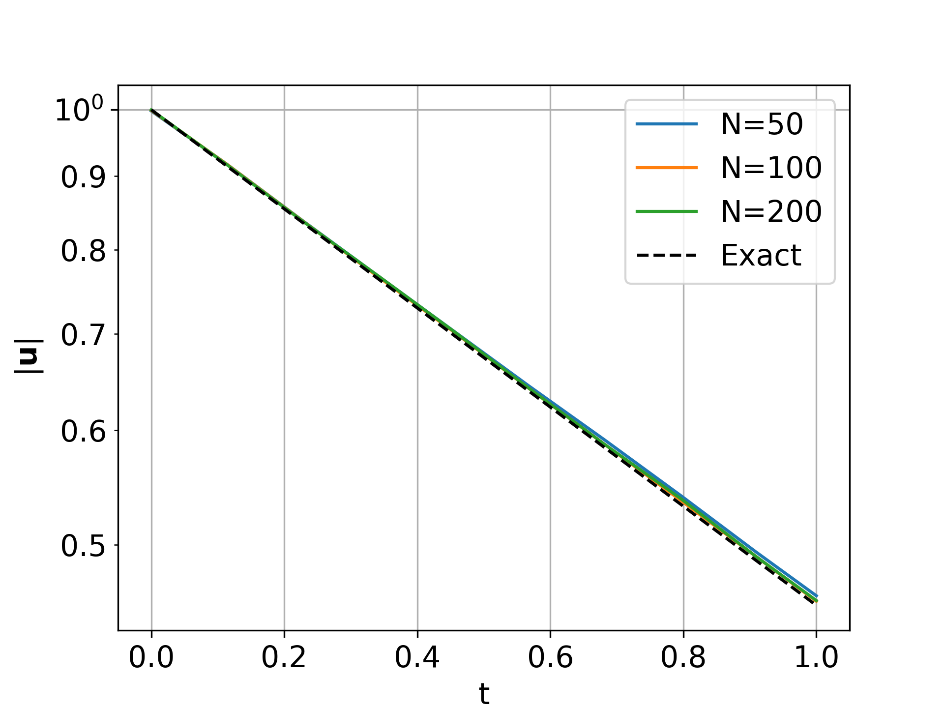
Figure 1: The decay in velocity magnitude for different resolutions compared with the exact solution for the Taylor-Green problem.

In fig. 1, we plot the decay in the velocity magnitude with time for different resolution compared with the exact solution. Clearly, the decay in the velocity magnitude is very close to the expected result.

In the lid-driven cavity problem, we consider a two-dimensional domain of size $1m\times 1m$ with 5 layers of ghost particles representing the solid particles. The top wall at $y=1m$ is given a velocity $u=1m/s$ along the x-direction. We solve the problem using the L-IPST-C scheme for different resolution for $10$ sec. However, we discretize the viscous term using the method given by Cleary and Monaghan (1999).

Figure 2: The velocity along $x$ and $y$ direction along the center line $x=0.5$ of the domain for the lid-driven cavity problem

In fig. 2, we plot the velocity along the centerline $x=0.5$ of the domain compared with the result of Ghia, Ghia, and Shin (1982). Clearly, the increase in resolution improves the accuracy.

We note that many researchers Ramachandran and Puri (2019); Adami, Hu, and Adams (2013); Oger et al. (2016); Huang et al. (2019); Damaziak and Malachowski (2019); Douillet-Grellier et al. (2019) use the above approach to verify their SPH schemes. Unfortunately, in both problems discussed above we used a discretization which is not second-order accurate. Evidently, these kind of verification techniques are unable to detect such issues. In addition, the simulations take a significant amount of time. For example, the $200\times 200$ resolution lid-driven cavity case took 150 minutes. In the case of the Taylor-Green problem since the exact solution is known one can evaluate the $L_{1}$ error in velocity or pressure.

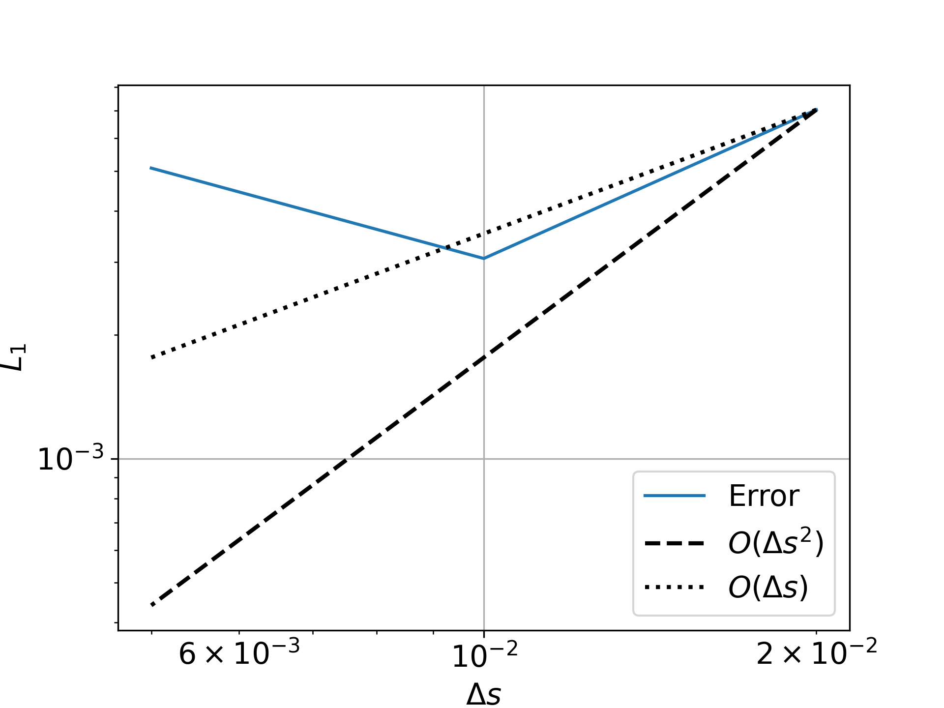
Figure 3: The $L_{1}$ error in velocity for the Taylor-Green problem.

In fig. 3, we plot the $L_{1}$ error in velocity as a function of particle spacing. The $L_{1}$ error is not second-order and diverges as we increase resolution from $100\times 100$ to $200\times 200$. However, this result does not suggest to us the exact reason for the error.

In general, one cannot exercise specific terms in the governing differential equation (GDE) in all the methods described above. Therefore, the source of error cannot be determined. For example, the solver may show convergence in the case of the Gresho-Chan vortex problem but fail for the Taylor-Green vortex problem due to an issue with the discretization of the viscous term. It is only recently Antuono (2020) that an analytic solution for three dimensional Navier-Stokes equations has been proposed. Other recent work Sharma and Sengupta (2019) has only focused on numerical investigation. It is therefore difficult to apply the MES in three dimensions. Furthermore, such studies require an even larger computational effort. Finally, we note that the Taylor-Green vortex problem is for an incompressible fluid making it difficult to test a WCSPH scheme.

Therefore, in the context of SPH, the comparison and MES techniques are insufficient and inefficient. We require a better method to verify the solver before proceeding to validation. The method of manufactured solutions offers exactly such a technique and this is described in the next section.

IV The Method of Manufactured Solutions

In conventional finite volume and finite element schemes, it is mandatory to demonstrate the order of convergence and the MMS has been used for this Choudhary et al. (2016b); Gfrerer and Schanz (2018); Waltz et al. (2014). For the SPH method, obtaining second-order convergence has itself been a challenge Vacondio et al. (2020) until recently Negi and Ramachandran (2021a). Moreover, to the best of our knowledge the MMS method has not been applied in the context of SPH. In this paper, we apply the principles of MMS to formally verify SPH solvers in a fast and reliable manner. The technique facilitates a careful investigation of the the various discretization operators, the boundary condition implementation, and time integrators.

In MMS, an artificial or manufactured solution is assumed. Let us assume the manufactured solution (MS) for $\Varrho$, $\mathbf{u}$, and $p$ in eq. 6 are $\tilde{\Varrho}$, $\tilde{\mathbf{u}}$, and $\tilde{p}$, respectively. Since the MS is not the solution of the eq. 6, we obtain a residue,

$$\begin{split}s_{\Varrho}&=\frac{d\tilde{\Varrho}}{dt}+\tilde{\Varrho}\nabla\cdot\mathbf{\tilde{u}},\\ \mathbf{s}_{\mathbf{u}}&=\frac{d\mathbf{\tilde{u}}}{dt}+\frac{\nabla\tilde{p}}{\tilde{\Varrho}}-\nu\nabla^{2}\mathbf{\tilde{u}},\\ \end{split}$$ (22)

where $s_{\Varrho}$ and $\mathbf{s}_{\mathbf{u}}$ are the residue term for continuity and momentum equation, respectively. Since, we have the closed form expression for all the terms in the RHS of the eq. 22, we may introduce the residue terms as source terms in the governing equations. We write the modified governing equations as

$$\begin{split}\frac{d\Varrho}{dt}&=-\Varrho\nabla\cdot\mathbf{u}+s_{\Varrho},\\ \frac{d\mathbf{u}}{dt}&=-\frac{\nabla p}{\Varrho}+\nu\nabla^{2}\mathbf{u}+\mathbf{s}_{\mathbf{u}}.\\ \end{split}$$ (23)

Finally, we solve the eq. 23. The addition of the source terms ensures that the solution is $\tilde{\Varrho}$, $\tilde{\mathbf{u}}$, and $\tilde{p}$.

One must take few precautions while employing the MMS Salari and Knupp (2000):

1. The MS must be $C^{n}$ smooth where $n$ is the order of the governing equations.

2. It must exercise all the terms i.e., for any evolution equation the MS cannot be time-independent.

3. The MS must be bounded in the domain of interest. For example, the MS $u=tan(x)$ in the domain $[-\pi,\pi]$ is not bounded thus, should not be used.

4. The MS should not prevent the successful completion of the code. For example, if the code assumes the solution to have positive pressure, then the MS must make sure that the pressure is not negative.

5. The MS should make sure that the solution satisfies the basic physics. For example, in a shear layer flow with discontinuous viscosity, the flux must be continuous.

We note that the MS may not be physically realistic.

We modify the basic steps for MMS proposed by Oberkampf and Roy (2010) for use in the context of WCSPH as follows:

1. Obtain the modified form of the governing equations as employed in the scheme. For example, in case of the $\delta$-SPH scheme Antuono et al. (2010), the continuity equation used is,

   $$\frac{d\Varrho}{dt}=-\Varrho\nabla\cdot\mathbf{u}+D\nabla^{2}\Varrho,$$ (24)

   where $D=\delta hc_{o}$ is the damping used, and $\delta$ is a numerical parameter. The additional diffusive term in eq. 24 must be retained while obtaining the source term.

2. Construct the MS using analytical functions. The general form of MS is given by

   $$f(x,y,t)=\phi_{o}+\phi(x,y,t),$$ (25)

   where $f$ is any property viz. $\Varrho$, $\mathbf{u}$, or $p$; $\phi_{o}$ is a constant, and $\phi(x,y,t)$ is a function chosen such that the five precautions listed above are satisfied.

3. Obtain the source term as done in eq. 22.

4. Add the source term in the solver appropriately. In SPH, the source term $s=s(x,y,z,t)$, is discretized as $s_{i}=s(x_{i},y_{i},z_{i},t)$ where subscript $i$ denotes the $i$^th particle.

5. Solve the modified equations using the solver for different particle spacings/smoothing length ($h$). The properties on the boundary particles are updated using the MS. We note that in the context of WCSPH schemes, one should not evaluate the derived quantities like gradient of velocity using the MS on the solid boundary.

6. Evaluate the discretization error for each resolution. We evaluate the error using

   $$L_{1}(h)=\sum_{j}\sum_{i}\frac{|f(\mathbf{x}_{i},t_{j})-f_{o}(\mathbf{x}_{i},t_{j})|}{N}\Delta t,$$ (26)

   where $f$ is the property of interest, $N$ is the total number of particles and $\Delta t$ is the time interval between consecutive solution instances.

7. Compute the order of accuracy and determine whether the desired order is achieved.

The solver involves discretization of the governing equations and appropriate implementation of the boundary conditions. The MMS can be used to determine the accuracy of both. However, to obtain the accuracy of boundary conditions, the order of convergence of the governing equations should be at least as large as that of the boundary conditionsChoudhary et al. (2016a). Bond et al. (2007) and Choudhary (2015) proposed a method to construct MS for boundary condition verification. In order to obtain a MS for a boundary surface given as $F(x,y,z)=C$, we multiply the original MS with $(C-F(x,y,z))^{m}$. We write the new MS as

$$f_{BC}(x,y,t)=\phi_{o}+(C-F(x,y,z))^{m}\phi(x,y,t),$$ (27)

where $m$ is the order of the boundary condition. For example, for the Dirichlet boundary $m=1$ and for Neumann boundary $m=2$.

In the next section, we demonstrate the application of MMS to obtain the order of convergence for the schemes listed in section II.

V Results

In this section, we apply the MMS to obtain the order of convergence of various schemes along with their boundary conditions. We first determine the initial particle configuration viz. unperturbed, perturbed, or packed Negi and Ramachandran (2021b) required for the MMS. We then demonstrate that one can apply the MMS to arbitrarily-shaped domains. We then compare the EDAC and PE-IPST-C schemes which differ in the treatment of the density. We next apply the MMS to E-C and TV-C schemes as they employ different governing equations compared to standard WCSPH in eq. 6. We also demonstrate the application of the MMS method as a technique to identify mistakes in the implementation. Finally, we employ the MMS to obtain the order of convergence of solid wall boundary conditions. We consider the boundary condition proposed by Maciá et al. (2011) for the demonstration.

In all our test cases, we use the quintic spline kernel with $h_{\Delta s}=h/{\Delta s}=1.2$, where $\Delta s$ is the initial inter-particle spacing. We consider a domain of size $1m\times 1m$. We simulate all the test cases for $50\times 50$, $100\times 100$, $200\times 200$, $250\times 250$, $400\times 400$, $500\times 500$, and $1000\times 1000$ resolutions to obtain the order of convergence plots. In all our simulations, we initialize the particles properties using the MS. We then solve eq. 23 and set the properties on any solid particle using the MS before every timestep. We set a fixed time step corresponding to the highest resolution for all the other resolutions. The appropriate time step is chosen using the criteria in eq. 11. We evaluate the $L_{1}$ error using eq. 26 in the solution.

The implementation of the code for the source terms (as shown in eq. 22) due to the MS are automatically generated using the sympy Meurer et al. (2017) and makoBayer et al. (06) packages. We recommend this approach to avoid mistakes during implementation. Salari and Knupp (2000) used a similar approach to automatically generate the source term for their solvers. We use the PySPH Ramachandran et al. (2020) framework for the implementation of the schemes described in this manuscript. All the figures and plots in this manuscript are reproducible with a single command through the use of the automan Ramachandran (2018) framework. The source code is available at https://gitlab.com/pypr/mms_sph.

V.1 The effect of initial particle configuration

The initial particle configuration plays a significant role in the error estimation since the divergence of the velocity is captured accurately when the particles are uniformly arranged Negi and Ramachandran (2021a). In this test case, we consider three different initial configurations of particles, widely used in SPH literature viz. unperturbed, perturbed, and packed. The unperturbed configuration is the one where we place the particles on a Cartesian grid such that the particles are at a constant distance along the grid lines. In the perturbed configuration, we perturb the particles initially placed on a Cartesian grid by adding a uniformly distributed random displacement as a fraction of the inter-particle spacing $\Delta s$. For the packed configuration, we use the method proposed in Colagrossi et al. (2012); Negi and Ramachandran (2021a) to resettle the particles from a randomly perturbed distribution to a new configuration such that the number density of the particles is nearly constant. In fig. 4, we show all the initial particle distributions with the solid boundary particles in orange.

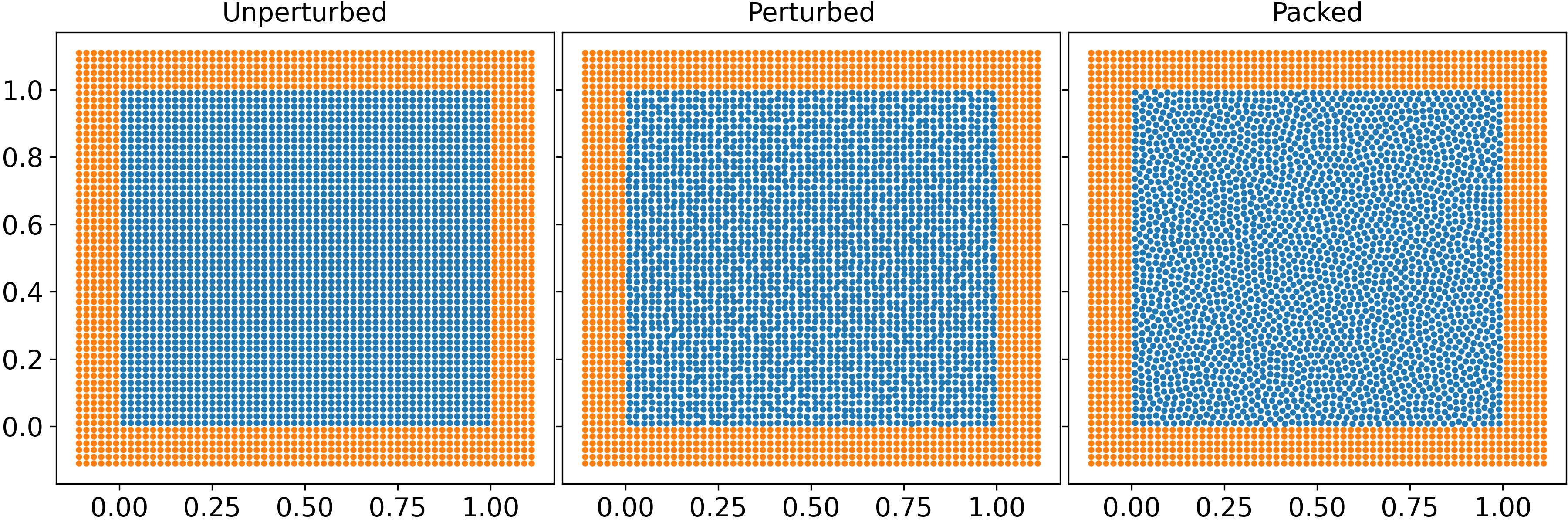
Figure 4: The different initial particle arrangements in blue with the solid boundary in orange.

We consider the MS of the form

$$\begin{split}u(x,y,t)=&e^{-10t}\sin{\left(2\pi x\right)}\cos{\left(2\pi y\right)}\\ v(x,y,t)=&-e^{-10t}\sin{\left(2\pi y\right)}\cos{\left(2\pi x\right)}\\ p(x,y,t)=&e^{-10t}\left(\cos{\left(4\pi x\right)}+\cos{\left(4\pi y\right)}\right)\\ \Varrho(x,y,t)=&\frac{p}{c_{o}^{2}}+\Varrho_{o}\\ \end{split}$$ (28)

where, we set $c_{o}=20m/s$ for all our testcases. The MS complies with all the required conditions discussed in section IV. We note that the MS chosen resembles the exact solution of the Taylor-Green problem. However, since the solver simulates the NS equation using a weakly compressible formulation, we obtain additional source terms when we substitute the MS to eq. 6 with $\nu=0.01m^{2}/s$. We obtain the source terms from the symbolic framework, sympy as,

$$\begin{split}s_{u}(x,y,t)=&2\pi ue^{-10t}\cos{\left(2\pi x\right)}\cos{\left(2\pi y\right)}-2\pi ve^{-10t}\sin{\left(2\pi x\right)}\sin{\left(2\pi y\right)}-10e^{-10t}\sin{\left(2\pi x\right)}\cos{\left(2\pi y\right)}+\\ ~{}&0.08\pi^{2}e^{-10t}\sin{\left(2\pi x\right)}\cos{\left(2\pi y\right)}-\frac{4\pi e^{-10t}\sin{\left(4\pi x\right)}}{\Varrho},\\ s_{v}(x,y,t)=&2\pi ue^{-10t}\sin{\left(2\pi x\right)}\sin{\left(2\pi y\right)}-2\pi ve^{-10t}\cos{\left(2\pi x\right)}\cos{\left(2\pi y\right)}-0.08\pi^{2}e^{-10t}\sin{\left(2\pi y\right)}\cos{\left(2\pi x\right)}+\\ ~{}&10e^{-10t}\sin{\left(2\pi y\right)}\cos{\left(2\pi x\right)}-\frac{4\pi e^{-10t}\sin{\left(4\pi y\right)}}{\Varrho},\\ s_{\Varrho}(x,y,t)=&-\frac{4\pi ue^{-10t}\sin{\left(4\pi x\right)}}{c_{0}^{2}}-\frac{4\pi ve^{-10t}\sin{\left(4\pi y\right)}}{c_{0}^{2}}-\frac{10\left(\cos{\left(4\pi x\right)}+\cos{\left(4\pi y\right)}\right)e^{-10t}}{c_{0}^{2}}.\\ \end{split}$$ (29)

We add $\mathbf{s}_{\mathbf{u}}=s_{u}\hat{\mathbf{i}}+s_{v}\hat{\mathbf{j}}$ to the momentum equation and $s_{\Varrho}$ to the continuity equation as shown in eq. 23. We solve the modified WCSPH equations in eq. 23 using the L-IPST-C method for 100 timesteps where we initialize the domain using eq. 28. The values of the properties $\mathbf{u}$, $p$, and $\Varrho$ on the (orange) solid particles are set using eq. 28 at the start of every time step.

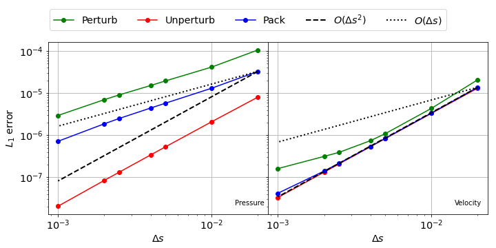
Figure 5: The error in pressure (left) and velocity (right) with fluid particles initialized using the MS in eq. 28 and the source term in eq. 29 after 10 timesteps for the different configurations.

In fig. 5, we plot the $L_{1}$ error in pressure and velocity after 10 timesteps as a function of resolution for different initial particle distributions. Clearly, the difference in initial configuration affects the error in pressure by a large amount. However, in velocity, the error is large in the case of the perturbed configuration only. The unperturbed configuration has zero divergence error at $t=0$ Negi and Ramachandran (2021a). Whereas, the perturbed configuration has high error due to the random initialization. Over the course of a few iterations, there is no significant difference between the distribution of particles for the unperturbed and the packed configurations. Therefore, we simulate the problems for 100 timesteps for a fair comparison.

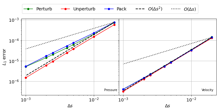
Figure 6: The error in pressure (left) and velocity (right) with fluid particles initialized using the MS in eq. 28 and the source term in eq. 29 after 100 timesteps for all the configurations.

In fig. 6, we plot the $L_{1}$ error in pressure and velocity after 100 timesteps as a function of resolution for the cases considered. Clearly, the difference in error is reduced. However, the order of convergence is not captured accurately. This is because the initial divergence is not captured accurately by the packed and perturbed configurations. This difference can be avoided through the use of a non-solenoidal velocity field. Therefore we consider the following modified MS,

$$\begin{split}u(x,y,t)=&y^{2}e^{-10t}\sin{\left(2\pi x\right)}\cos{\left(2\pi y\right)}\\ v(x,y,t=&-e^{-10t}\sin{\left(2\pi y\right)}\cos{\left(2\pi x\right)}\\ p(x,y,t)=&\left(\cos{\left(4\pi x\right)}+\cos{\left(4\pi y\right)}\right)e^{-10t}\\ \end{split}$$ (30)

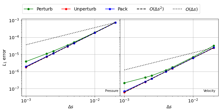
Figure 7: The error in pressure (left) and velocity (right) with fluid particles initialized using the MS in eq. 30 and the corresponding source terms after 100 timesteps for all the configurations.

We note that the new MS velocity field is not divergence-free. We obtain the source term with $\nu=0.01m^{2}/s$ as done in eq. 29. We simulate the problem by initializing the domain using MS in eq. 30. We also update the solid boundary properties using this MS before every timestep. In fig. 7, we plot the $L_{1}$ error for pressure and velocity as a function of resolution. Clearly, both the packed and unperturbed domain show second-order convergence. Whereas, the perturbed configuration fails to show second-order convergence. Therefore, in the context of WCSPH schemes, one should not use a divergence-free field in the MS. Furthermore, one should use either a packed or unperturbed configuration for the convergence study.

It is important to note that in stark contrast the Taylor-Green vortex problem the method shows second-order convergence irrespective of the value of $c_{o}$. In Negi and Ramachandran (2021b) a much higher $c_{o}=80m/s$ was necessary in order to demonstrate second-order convergence. Furthermore, the convergence is independent of the initial configuration after 100 steps; therefore, we recommend simulating all the testcases for at least 100 timesteps to obtain the true order of convergence. It is important to note that some discretizations are second-order accurate when an unperturbed configuration is used Negi and Ramachandran (2021a). In order to test the robustness of the discretization we recommend using a packed configuration.

V.2 The selection of the domain shape

We now show the effect of the shape of the domain on the convergence of a scheme. We consider a square-shaped and a butterfly-shaped domain as shown in fig. 8.

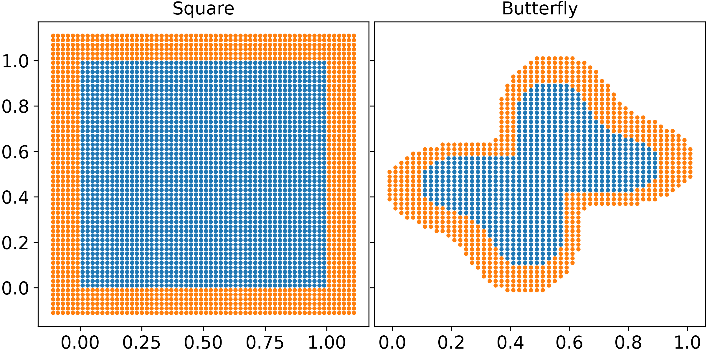
Figure 8: The different domain shapes with solid particles in orange and fluid particles in blue.

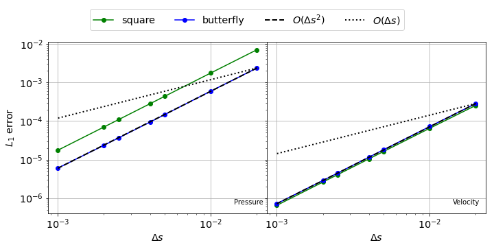
Figure 9: The $L_{1}$ error in pressure (left) and velocity (right) with increase in resolution for different shapes of the domain.

We consider the MS with the non-solenoidal velocity field in eq. 30 as used in the previous testcase. The source terms obtained remains same as before, where we consider $\nu=0.01m^{2}/s$. We solve the modified equations using the L-IPST-C scheme for 100 time step for each domain. We initialize the fluid and solid particles using the MS in eq. 30. We update the properties of the solid particles before every timestep using the same MS.

In fig. 9, we show the convergence of $L_{1}$ error after 100 timesteps in pressure and velocity as a function of resolution for both the domain considered. Clearly, both the domains considered show second-order convergence. Hence, one can consider any shape of the domain for the convergence study of WCSPH schemes using MMS. However, we only use square-shaped domain for all our test cases.

V.3 Comparison of EDAC and PE-IPST-C

In this testcase, we compare the convergence of EDAC Ramachandran and Puri (2019) and PE-IPST-C Negi and Ramachandran (2021a) schemes. These two schemes have two major differences. First, the discretizations used in PE-IPST-C method are all second-order accurate in contrast to the EDAC scheme. Second, the volume of the fluid given by

$$V_{i}=\frac{1}{\sum_{j}W_{ij}},$$ (31)

is used in the discretization of the term $\frac{\nabla p}{\Varrho}$ whereas, in PE-IPST-C the density $\Varrho$ is independent of neighbor particle positions. We evaluate $\Varrho$ using a linear equation of state, eq. 14

In the EDAC scheme the initial configuration of particles affects the results. Therefore, we consider an unperturbed configuration as shown in fig. 4. In order to reduce the complexity, we consider an inviscid MS given by

$$\begin{split}u(x,y)=&\sin{\left(2\pi x\right)}\cos{\left(2\pi y\right)}\\ v(x,y)=&-\sin{\left(2\pi y\right)}\cos{\left(2\pi x\right)}\\ p(x,y)=&\cos{\left(4\pi x\right)}+\cos{\left(4\pi y\right)}.\\ \end{split}$$ (32)

Thus, the solver must maintain the pressure and velocity fields in the absence of the viscosity. The source term for the EDAC scheme is given by

$$\begin{split}s_{u}(x,y)=&2\pi u\cos{\left(2\pi x\right)}\cos{\left(2\pi y\right)}-2\pi v\sin{\left(2\pi x\right)}\sin{\left(2\pi y\right)}-\frac{4\pi\sin{\left(4\pi x\right)}}{\rho}\\ s_{v}(x,y)=&2\pi u\sin{\left(2\pi x\right)}\sin{\left(2\pi y\right)}-2\pi v\cos{\left(2\pi x\right)}\cos{\left(2\pi y\right)}-\frac{4\pi\sin{\left(4\pi y\right)}}{\rho}\\ s_{p}(x,y)=&-1.25h\left(-16\pi^{2}\cos{\left(4\pi x\right)}-16\pi^{2}\cos{\left(4\pi y\right)}\right)-4\pi u\sin{\left(4\pi x\right)}-4\pi v\sin{\left(4\pi y\right)}.\\ \end{split}$$ (33)

We note that the source term employs density $\rho$ which is a function of particle position given by $\frac{m_{i}}{V_{i}}$, where $m_{i}$ is the mass of the particle. In the case of the PE-IPST-C scheme, the source term is given by

$$\begin{split}s_{u}(x,y)=&2\pi u\cos{\left(2\pi x\right)}\cos{\left(2\pi y\right)}-2\pi v\sin{\left(2\pi x\right)}\sin{\left(2\pi y\right)}-\frac{4\pi\sin{\left(4\pi x\right)}}{\Varrho}\\ s_{v}(x,y)=&2\pi u\sin{\left(2\pi x\right)}\sin{\left(2\pi y\right)}-2\pi v\cos{\left(2\pi x\right)}\cos{\left(2\pi y\right)}-\frac{4\pi\sin{\left(4\pi y\right)}}{\Varrho}\\ s_{p}(x,y)=&-1.25h\left(-16\pi^{2}\cos{\left(4\pi x\right)}-16\pi^{2}\cos{\left(4\pi y\right)}\right)-4\pi u\sin{\left(4\pi x\right)}-4\pi v\sin{\left(4\pi y\right)}.\\ \end{split}$$ (34)

We note that the source term $s_{p}$ in eq. 33 and eq. 34 are same. We simulate the problem with the MS in eq. 32. The (orange) solid boundary properties are reset using this MS before every time step.

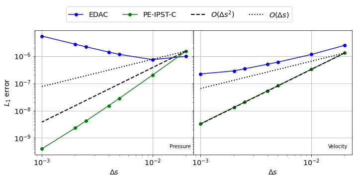
Figure 10: The error in pressure (left) and velocity (right) with fluid particles initialized using the MS in eq. 32, and the source term in eq. 33 for EDAC and eq. 34 for PE-IPST-C after 1 timestep.

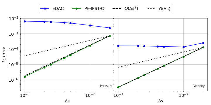
Figure 11: The error in pressure (left) and velocity (right) with fluid particles initialized using the MS in eq. 32, and the source term in eq. 33 for EDAC and eq. 34 for PE-IPST-C after 100 timestep.

In fig. 10, we plot the $L_{1}$ error in pressure and velocity after one timestep for both the schemes. Clearly, the EDAC case diverges in the case of pressure, whereas we observe a reduced order of convergence in velocity. In contrast, the PE-IPST-C scheme shows second-order convergence in velocity and higher in case of pressure. We observe this increased order only for the first iteration. In fig. 11, we plot the $L_{1}$ error in pressure and velocity after 100 timesteps for both the schemes. In the case of the EDAC scheme, the order of convergence in the velocity does not remains first-order whereas, the L-IPST-C scheme shows second-order convergence in both pressure and velocity.

We note that, we use an unperturbed mesh therefore we must obtain second-order convergence to the level of discretization error for 1 timestep in the case of the EDAC scheme as well. We observe this behavior since $\rho$ (a function of neighbor particle positions) is present in the source term which comes from the governing differential equation. Therefore, as mentioned in Negi and Ramachandran, 2021a, we should treat $\rho$ as a separate property as we do in the case of the PE-IPST-C scheme.

V.4 Comparison of E-C and TV-C

In this test case, we apply MMS to E-C and TV-C schemes introduced in section II. The governing equations for E-C scheme is given in eq. 17 whereas for TV-C in eq. 15. The expression for the source terms turns out to be same for both eq. 17 and eq. 15 governing equations given by

$$\begin{split}s_{\Varrho}=&\frac{\partial\Varrho}{\partial t}+\Varrho\nabla\cdot\mathbf{u}+\mathbf{u}\cdot\nabla\Varrho,\\ s_{\mathbf{u}}=&\frac{\partial\mathbf{u}}{\partial t}+\frac{\nabla p}{\Varrho}-\nu\nabla^{2}\mathbf{u}+\mathbf{u}\cdot\nabla\mathbf{u}.\\ \end{split}$$ (35)

These source terms are the same as obtained in the case of the L-IPST-C scheme as well. In E-C scheme, we fix the grid and add the convective term as the correction, whereas in TV-C scheme, we add the shifting velocity in the LHS of the governing equations.

In order to show the convergence of the scheme, we consider the inviscid MS in eq. 32 with the linear EOS. We do not consider the viscous term since the term introduces similar error in both the schemes. We write the source term as

$$\begin{split}s_{u}(x,y)=&2\pi u\cos{\left(2\pi x\right)}\cos{\left(2\pi y\right)}-2\pi v\sin{\left(2\pi x\right)}\sin{\left(2\pi y\right)}-\frac{4\pi\sin{\left(4\pi x\right)}}{\Varrho},\\ s_{v}(x,y)=&2\pi u\sin{\left(2\pi x\right)}\sin{\left(2\pi y\right)}-2\pi v\cos{\left(2\pi x\right)}\cos{\left(2\pi y\right)}-\frac{4\pi\sin{\left(4\pi y\right)}}{\Varrho},\\ s_{\Varrho}(x,y)=&-\frac{4\pi u\sin{\left(4\pi x\right)}}{c_{0}^{2}}-\frac{4\pi v\sin{\left(4\pi y\right)}}{c_{0}^{2}},\\ \end{split}$$ (36)

where $\mathbf{s}_{\mathbf{u}}=s_{u}\hat{\mathbf{i}}+s_{u}\hat{\mathbf{j}}$ is the source term for the momentum equation in both the schemes. We consider an unperturbed initial particle distribution and run the simulation for 100 timesteps. The particles are initialized with the MS in eq. 32 and solid boundary are reset using the MS before every time step.

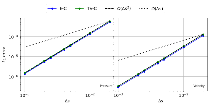
Figure 12: The error in pressure (left) and velocity (right) with fluid particles initialized using the MS in eq. 32 and the source term in eq. 36 after 100 timesteps for the different schemes.

In fig. 12, we plot the $L_{1}$ error in pressure and velocity as a function of resolution for both the schemes. Since we use second-order accurate discretization in both the schemes, they show second-order convergence in both pressure and velocity as expected. Thus, we see that the modified governing equations (eq. 15 and eq. 17) must be considered to obtain the source term for the schemes.

V.5 Identification of mistakes in the implementation

In this section, we demonstrate the use of MS as a technique to identify mistakes in the implementation. We use the L-IPST-C scheme, and introduce either erroneous or lower order discretization for a single term in the governing equations. We then use the proposed MMS to identify the problem.

V.5.1 Wrong divergence estimation

We introduce an error in the discretized form of the continuity equation used in the L-IPST-C scheme. We refer to this modified scheme as incorrect CE. We write the incorrect discretization for the divergence of velocity as

$$\left<\nabla\cdot\mathbf{u}\right>=\sum_{j}(\mathbf{u}_{j}{\color[rgb]{1,0,0}+}\mathbf{u}_{i})\cdot\tilde{\nabla}W_{ij}\omega_{j},$$ (37)

where the error is shown in red. Since only the continuity equation is involved, we use the inviscid MS given by

$$\begin{split}u(x,y)=&\left(y-1\right)^{2}\sin{\left(2\pi x\right)}\cos{\left(2\pi y\right)}\\ v(x,y)=&-\sin{\left(2\pi y\right)}\cos{\left(2\pi x\right)}\\ p(x,y)=&\left(y-1\right)\left(\cos{\left(4\pi x\right)}+\cos{\left(4\pi y\right)}\right)\\ \end{split}$$ (38)

The source terms can be determined by subjecting the above MS to eq. 6. We simulate the problem for 1 timestep with a packed domain (see fig. 4). In order to test erroneous or lower order discretization in the scheme, we recommend the simulation of only one timestep with a packed initial particle distribution.

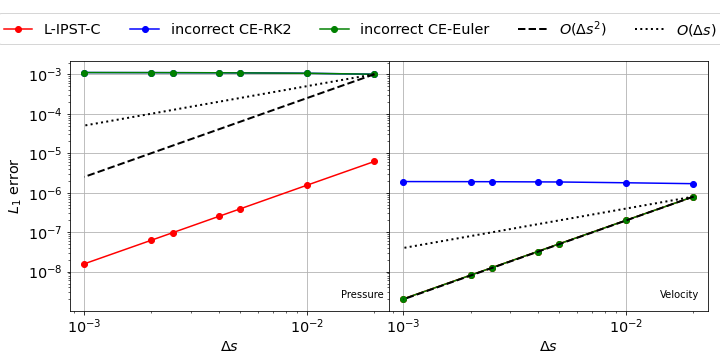
Figure 13: The error in pressure (left) and velocity (right) with fluid particles initialized using the MS in eq. 32 and the source term in eq. 36 after 1 timestep for L-IPST-C and the scheme with the divergence computed using the incorrect eq. 37.

In fig. 13, we plot the $L_{1}$ error in pressure and velocity as a function of the resolution for the L-IPST-C scheme and its variant incorrect CE with two time integrators, Euler and RK2. Clearly, the error in pressure increases by a significant amount and the order of convergence is zero for incorrect CE. However, the error in pressure propagates to velocity in case of the RK2 integrator. Therefore, we recommend that one use single stage integrators while using MMS as a technique to identify mistakes. By looking at incorrect CE-Euler plot in fig. 13 we can immediately infer that there is an error in either the continuity equation or the equation of state.

V.5.2 Using a symmetric pressure gradient discretization

In this testcase, we use a symmetric formulation as used by Monaghan, 2005; Sun et al., 2017; Negi and Ramachandran, 2021a for the pressure gradient term in the L-IPST-C scheme. We refer to this method as sym. Since only the pressure gradient is involved, we use the same MS as in the previous case.

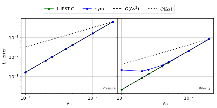
Figure 14: The error in pressure (left) and velocity (right) with fluid particles initialized using the MS in eq. 32 and the source term in eq. 36 after 1 timestep for L-IPST-C and the scheme with pressure gradient computed using symmetric formulation.

In fig. 14, we plot the $L_{1}$ error after 1 timestep in pressure and velocity as a function of resolution for L-IPST-C and sym schemes. Clearly, the order of convergence is affected in the velocity only. Therefore, it is evident that a inconsistent pressure gradient discretization is used.

V.5.3 Using inconsistent discrete viscous operator

In this testcase, we use the formulation proposed by Cleary and Monaghan (1999) to approximate the viscous term in the L-IPST-C scheme. We refer to this method as Cleary. Since viscosity is involved, we use the MS involving viscous effect given by eq. 30. While testing the viscous term we use a high value of $\nu=.25m^{2}/s$ such that the error due to viscosity dominates the error in the momentum equation. We simulate the problem with a packed configuration of particles for 1 timestep using the MS in eq. 30 and with the corresponding source terms. We fix the timestep using eq. 11 such that we satisfy the stability condition.

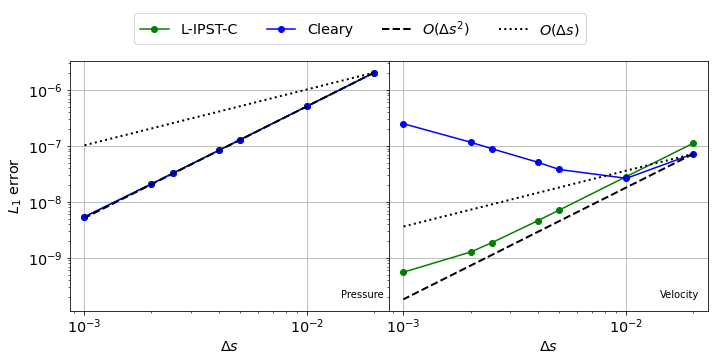
Figure 15: The error in pressure (left) and velocity (right) with fluid particles initialized using the MS in eq. 30 and the corresponding source term after 1 timestep for L-IPST-C and the scheme with viscous term discretized using formulation given by Cleary and Monaghan (1999).

In fig. 15, we plot the $L_{1}$ error in pressure and velocity as a function of resolution for L-IPST-C and Cleary schemes. Since the viscous formulation by Cleary and Monaghan (1999) does not converge in the perturbed domain Negi and Ramachandran (2021a), we observe divergence in the velocity. Therefore, we infer that there is an error in the viscous term.

V.6 MMS applied to boundary condition

In this section, we use MMS to verify the convergence of boundary conditions in SPH. In order to do this, the scheme used must converge at least as fast as the boundary conditions. Therefore, we consider the second-order convergent L-IPST-C scheme. We study the Dirichlet boundary conditions for pressure and velocity, no-slip and slip velocity boundary conditions, and the Neumann pressure boundary condition. We consider an unperturbed domain as shown in fig. 16, where we solve the fluid equations using the L-IPST-C scheme for the blue particles and set the MS before every time step for the green particles. We set the properties in the orange particles using the appropriate boundary condition we intend to test. For example, if we set the pressure Dirichlet boundary condition in SPH then we set velocity and density using the MS.

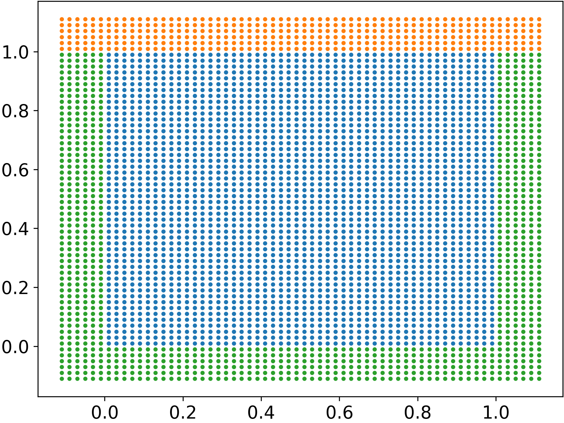
Figure 16: Different particle used for testing the boundary condition with fluid in blue, MS solid boundary in green, and SPH solid boundary in orange.

In order to obtain rate of convergence, we evaluate $L_{\infty}$ error using,

$$L_{\infty}(N)=max\{|f(\mathbf{x}_{i})-f(\mathbf{x}_{o})|,i=1,\dots,N\},$$ (39)

where N is the total number of fluid particles for which $y>0.9$, and $f(\mathbf{x}_{i})$ and $f(\mathbf{x}_{o})$ are the computed and exact value of the property of interest, respectively. We consider only a portion near the boundary since only that region is affected the most by the boundary implementation. In the following sections, we test the different boundary conditions in SPH using MMS.

V.6.1 Dirichlet boundary condition

In this testcase, we construct the MS for boundary condition as discussed in section IV. In order to set the homogenous boundary condition at $y=1$, we modify the MS in eq. 32 as

$$\begin{split}u=&\left(y-1\right)\sin{\left(2\pi x\right)}\cos{\left(2\pi y\right)}\\ v=&-\left(y-1\right)\sin{\left(2\pi y\right)}\cos{\left(2\pi x\right)}\\ p=&\left(y-1\right)\left(\cos{\left(4\pi x\right)}+\cos{\left(4\pi y\right)}\right)\\ \end{split}$$ (40)

Clearly, at $y=1$ we have boundary values $u=v=p=0$. In SPH, the Dirichlet boundary may be applied by setting the desired value of the property on the ghost layer shown in orange in fig. 16. We set homogenous velocity and pressure boundary conditions in two separate testcases and refer to them as velocity BC and pressure BC, respectively. We set the pressure/velocity on the solid using the MS when we set velocity/pressure using the SPH method. We simulate the problem for 100 timesteps with the MS in eq. 40.

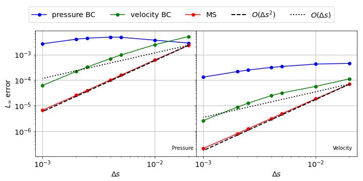
Figure 17: The error in pressure (left) and velocity (right) with fluid particles initialized using the MS in eq. 40 100 timesteps for L-IPST-C and velocity BC and pressure BC applied at the orange boundary in fig. 16.

In fig. 17, we plot the $L_{\infty}$ error in pressure and velocity as a function of resolution for L-IPST-C, velocity BC, and pressure BC. Clearly, both the boundary conditions introduce error in the solution. The error introduced due to Velocity BC remains around second-order in pressure and first-order in velocity. The pressure BC is rarely used in SPH and introduces a significant amount of error with almost zero order convergence.

V.6.2 Slip boundary condition

In the SPH method, the slip boundary condition can be applied using the method proposed by Maciá et al. (2011). First, we extrapolate the velocity of the fluid to the solid using

$$\mathbf{u}_{s}=\frac{\sum\mathbf{u}_{f}W_{sf}}{\sum_{j}W_{sf}},$$ (41)

where $\mathbf{u}_{s}$ and $\mathbf{u}_{f}$ denotes the velocity of wall and fluid particles, respectively. Then, we reverse the component of the velocity normal to the wall. This method ensures that the divergence of velocity is captured accurately near the slip wall. Therefore, we consider the inviscid MS given by

$$\begin{split}u(x,y)=&\left(y-1\right)^{2}\sin{\left(2\pi x\right)}\cos{\left(2\pi y\right)}\\ v(x,y)=&-\sin{\left(2\pi y\right)}\cos{\left(2\pi x\right)}\\ p(x,y)=&\left(y-1\right)\left(\cos{\left(4\pi x\right)}+\cos{\left(4\pi y\right)}\right)\\ \end{split}$$ (42)

We note that the $u$ velocity is symmetric across $y=1$ and $v$ velocity is asymmetric. We consider the domain as shown in fig. 16 and apply the free slip boundary condition on the solid boundary shown in orange color for the L-IPST-C scheme. We refer to this method as slip BC. We note that the pressure and density on the solid is set using the MS. We simulate the problem for 100 timesteps.

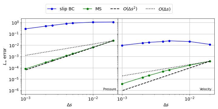
Figure 18: The error in pressure (left) and velocity (right) with fluid particles initialized using the MS in eq. 42 after 100 timesteps for L-IPST-C and slip BC applied on the orange boundary in fig. 16.

In fig. 18, we plot the $L_{1}$ error in pressure and velocity as a function of resolution for L-IPST-C and slip BC schemes. Clearly, the application of slip boundary condition increases the error and the order of convergence is less than one. In the case of the L-IPST-C scheme, the lower resolutions show first order convergence but as the resolution increases approaches second-order. We note that the fig. 18 shows the $L_{\infty}$ error, however convergence of the $L_{1}$ error is close to second-order for all resolutions. In summary, the slip boundary condition as proposed in Maciá et al., 2011 is accurate in velocity but reduces the accuracy of the pressure.

V.6.3 Pressure boundary condition

In the pressure boundary condition proposed by Maciá et al. (2011), we ensure that the pressure gradient normal to the boundary is zero. We apply the boundary condition by setting the pressure of the solid boundary particles using

$$p_{s}=\frac{\sum p_{f}W_{sf}}{\sum_{j}W_{sf}},$$ (43)

where $p_{s}$ and $p_{f}$ denotes the pressure of wall and fluid particles, respectively. For simplicity, we ignore the acceleration due to gravity and motion of the solid body. We consider the MS of the form

$$\begin{split}u(x,y)=&y^{2}\sin{\left(2\pi x\right)}\cos{\left(2\pi y\right)}\\ v(x,y)=&-\sin{\left(2\pi y\right)}\cos{\left(2\pi x\right)}\\ p(x,y)=&\left(y-1\right)^{2}\left(\cos{\left(4\pi x\right)}+\cos{\left(4\pi y\right)}\right)\\ \end{split}$$ (44)

Clearly, the MS satisfies $\frac{\partial p}{\partial y}=0$ at $y=1$. We consider the domain as shown in fig. 16 and apply the pressure boundary condition on the solid boundary shown in orange color for L-IPST-C scheme. We refer to this method as Neumann BC. We simulate the problem for 100 timesteps.

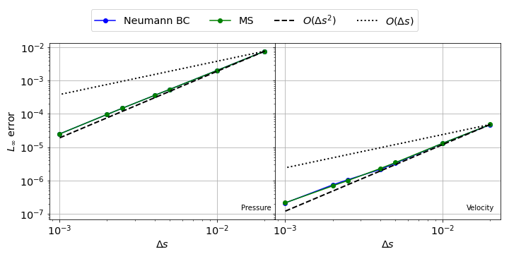
Figure 19: The error in pressure (left) and velocity (right) with fluid particles initialized using the MS in eq. 44 after 100 timesteps for L-IPST-C and Neumann BC applied on the orange boundary in fig. 16.

In fig. 19, we plot the $L_{\infty}$ error in pressure and velocity for L-IPST-C and Neumann BC. The results show that the pressure boundary condition is second order convergent.

V.6.4 No-slip boundary condition

Maciá et al. (2011) proposed the no-slip boundary condition for SPH where we set the wall velocity as

$$\mathbf{u}_{s}=2\mathbf{u}_{w}-\mathbf{\tilde{u}}_{s},$$ (45)

where $\mathbf{u}_{w}$ is velocity of the wall and $\mathbf{\tilde{u}}_{s}$ is the Shepard interpolated velocity (see eq. 41). In the no-slip boundary, we ensure that $\frac{\partial u}{\partial y}=0$ at $y=1$ therefore, we use the MS for viscous flow given by

$$\begin{split}u(x,y,t)=&\left(y-1\right)^{2}e^{-10t}\sin{\left(2\pi x\right)}\cos{\left(2\pi y\right)}\\ v(x,y,t)=&-\left(y-1\right)^{2}e^{-10t}\sin{\left(2\pi y\right)}\cos{\left(2\pi x\right)}\\ p(x,y,t)=&\left(\cos{\left(4\pi x\right)}+\cos{\left(4\pi y\right)}\right)e^{-10t}\\ \end{split}$$ (46)

We consider the domain as shown in fig. 16 and apply the pressure boundary condition on the solid boundary shown in orange color for the L-IPST-C scheme. We refer to this method as no-slip BC. We simulate the problem for 100 timesteps with $\nu=1.0m^{2}/s$.

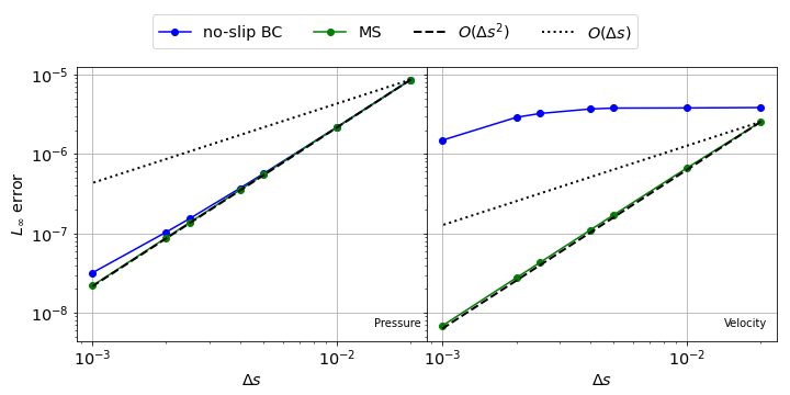
Figure 20: The error in pressure (left) and velocity (right) with fluid particles initialized using the MS in eq. 44 after 100 timesteps for L-IPST-C and no-slip BC applied on the orange boundary in fig. 16.

In fig. 20, we plot the $L_{\infty}$ error in pressure and velocity for 100 timesteps. Clearly, the no-slip BC shows increased error and a zero-order convergence. However, it does not introduce error in the pressure.

Thus in this section, we have demonstrated the MMS for obtaining the order of convergence of boundary condition implementations in SPH.

V.7 Convergence and extreme resolutions

Thus far we have used particle resolutions in the range $10^{-3}\leq\Delta s\leq 2\times 10^{-2}$. We wish to study the convergence of the scheme when much higher resolutions are considered. We consider a domain of size $1\times 1$ with uniformly distributed particles as shown in fig. 21. In order to reduce computation, we reduce the size of the domain by half if the number of particles crosses $1M$. In the fig. 21, the red box shows the domain considered for the computation which one million particles with $\Delta s=1.25\times 10^{-4}$. In order to obtain an unbiased error estimate we consider same MS and the domain shown by black box in fig. 21 to evaluate $L_{\infty}$ error using eq. 39.

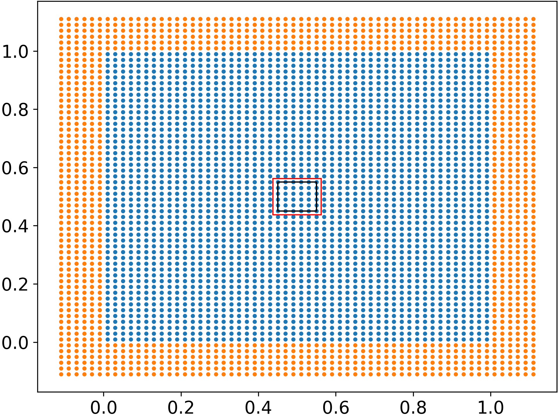
Figure 21: The domain filled by blue fluid particles. The red box shows the smallest domain considered for the highest resolution of $8000\times 8000$ and the black box shows the area which is considered to evaluate error for all the resolutions.

We first consider the MS given in eq. 30. We solve the eq. 23 using the L-IPST-C scheme for all the resolutions with $\nu=.01m^{2}/s$. We consider the case where we do not correct the kernel gradient in the discretization of eq. 23 in the L-IPST-C scheme.

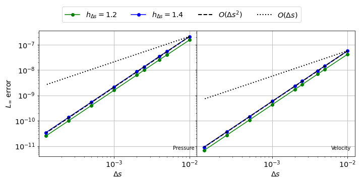
Figure 22: The error in pressure (left) and velocity (right) as a function of resolution for two different $h_{\Delta s}$ values with the MS in eq. 30. All cases are solved using L-IPST-C scheme with kernel gradient correction.

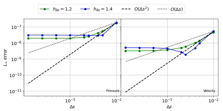
Figure 23: The error in pressure (left) and velocity (right) as a function of resolution for two different $h_{\Delta s}$ values with the MS in eq. 30. All cases are solved using L-IPST-C scheme with no kernel gradient correction.

In fig. 22, we plot the error in pressure and velocity solved using L-IPST-C scheme with kernel gradient corrected, after 100 timesteps as a function of resolution for $h_{\Delta s}=1.2$ and $h_{\Delta s}=1.4$. Clearly, We obtain second order convergence. In fig. 23, we plot the error for the case where we do not employ kernel gradient correction. Clearly, the discretization error dominates.

We also consider the MS containing a range of frequencies given by

$$\begin{split}u(x,y,t)=&y^{2}e^{-10t}\sum_{j=1}^{10}\sin{\left(2j\pi x\right)}\cos{\left(2j\pi y\right)}\\ v(x,y,t)=&-e^{-10t}\sum_{j=1}^{10}\sin{\left(2j\pi y\right)}\cos{\left(2j\pi x\right)}\\ p(x,y,t)=&e^{-10t}\sum_{j=1}^{10}\cos{\left(4j\pi x\right)}+\cos{\left(4j\pi y\right)}.\\ \end{split}$$ (47)

We simulate the eq. 6 using L-IPST-C scheme for the above MS. As before, we also consider the case where we do not employ kernel correction.

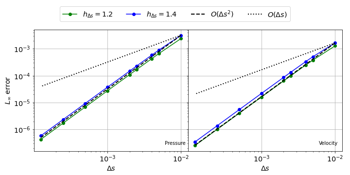
Figure 24: The error in pressure (left) and velocity (right) as a function of resolution for two different $h_{\Delta s}$ values with the MS in eq. 47. All cases are solved using L-IPST-C scheme with kernel gradient correction.

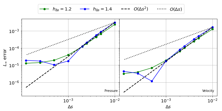
Figure 25: The error in pressure (left) and velocity (right) as a function of resolution for two different $h_{\Delta s}$ values with the MS in eq. 47. All cases are solved using L-IPST-C scheme with no kernel gradient correction.

In fig. 24, we plot the error in pressure and velocity solved using L-IPST-C scheme with kernel gradient correction for 100 timesteps as a function of resolutions. Clearly, both the cases shows second-order convergence. In fig. 25, we plot the error in pressure and velocity for the solution obtained using L-IPST-C scheme with no kernel correction. As can be seen the kernel correction is essential in order to obtain second-order convergence at high resolutions.

We have therefore shown that we can consider very high resolutions using the MMS technique. This enables us to find flaws in the scheme which may not converge at very high resolution. These are hard to test using traditional methods where an actual problem is solved.

V.8 Verification in 3D

We now use the MMS to verify a three dimensional solver. Since the number of particles in three-dimensions increase much faster than in two-dimensions, we can reduce the domain size with resolution as done while dealing with extreme resolutions. We consider a unit cube domain size with 1 million particles. As we increase the resolution, we decrease the size of the domain such that the number of particles in the domain remains at 1 million. We consider the MS given by

$$\begin{split}u(x,y,z,t)=&y^{2}e^{-10t}\sin{\left(\pi\left(2x+2z\right)\right)}\cos{\left(\pi\left(2x+2y\right)\right)}\\ v(x,y,z,t)=&-e^{-10t}\sin{\left(\pi\left(2y+2z\right)\right)}\cos{\left(\pi\left(2x+2y\right)\right)}\\ w(x,y,z,t)=&-e^{-10t}\sin{\left(\pi\left(2x+2z\right)\right)}\cos{\left(\pi\left(2y+2z\right)\right)}\\ p(x,y,z,t)=&\left(\cos{\left(\pi\left(4x+4y\right)\right)}+\cos{\left(\pi\left(4x+4z\right)\right)}\right)e^{-10t}.\\ \end{split}$$ (48)

We obtain the source term by subjecting the MS in eq. 48 to the governing equation in eq. 6 with $\nu=0.01m^{2}/s$. We simulate the problem for 10 timesteps.

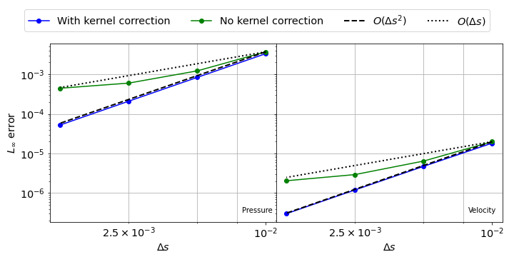
Figure 26: The $L_{\infty}$ error in pressure (left) and velocity (right) after 10 timesteps as a function of resolution solved using L-IPST-C scheme with and without kernel correction. The source term are calculated using the MS in eq. 48.

In fig. 26, we plot the $L_{\infty}$ error in pressure and velocity as a function of resolution for L-IPST-C scheme with and without kernel correction. As expected, the case with no kernel correction gradually flatten due dominance of discretization error. The case with kernel correction shows second order convergence in both pressure and velocity. Thus we see that we can easily test the SPH method in a three-dimensional domain using the MMS.

VI Discussion

We have used the MMS to verify the convergence of different WCSPH schemes. Thus far, most of the numerical studies of the accuracy and convergence of the WCSPH method have used either an exact solution like the Taylor-Green vortex problem, or with an established solver, or experimental result. These methods are therefore limited in their ability to detect specific problems in an SPH implementation. This is true even in the recent work of Negi and Ramachandran (2021a) where a Taylor-Green problem and a Gresho-Chan vortex problem is used. These are complex problems and obtaining a solution to these involves a significant amount of computation. Moreover, if the results do not produce the expected accuracy or convergence, the researcher does not obtain much insight into the origin of the problem. Furthermore, the established approaches do not offer any means to study the accuracy of boundary condition implementations.

In this context, the proposed approach offers a multitude of advantages listed and discussed below:

• The method is highly efficient in terms of execution time. We are able to detect problems in the implementations of specific discretization operators in less than 100 iterations. Even for our most challenging cases with a million particles, the typical run time for a single computation on a multi-core CPU does not exceed a few minutes. On the other hand, the comparison study for the lid-driven cavity case in section III took 150 minutes for the $200\times 200$ resolution.

• The method easily works in three dimensions and we demonstrate its applicability for a simple three-dimensional case. This is significant because traditional SPH verifications only use two-dimensional problems.

• We can effectively test the boundary condition implementations through this method. In this work we have demonstrated this for Dirichlet and Neumann boundary conditions in both pressure and velocity.

• The method allows us to identify very specific problems with a solver. Through a judicious choice of MS and time integrator, we can identify if the implementation of a specific governing equation is the source of a problem. We have demonstrated this with several examples in the preceding sections.

• We are able to verify the order of convergence efficiently even for very high resolutions and thereby test if the scheme is truly second order convergent as the resolution increases. In the present work we have demonstrated this for extremely high resolutions (involving $8000\times 8000$ particles) without needing to simulate the problem for a long duration and also limiting the number of computational particles to a smaller number.

• The method will work on any manufactured solution and this allows us to test the scheme with functions involving a large range of frequencies. In contrast, many exact solutions involve simple functional forms. Therefore by using the MMS the solver can be tested with a more challenging class of problems.

As a result of these significant advantages, the proposed method offers a robust, efficient, and powerful method to verify the accuracy and convergence of SPH schemes.

VII Conclusions

In this paper we propose the use of the method of manufactured solutions (MMS) in order to verify an SPH solver. While the MMS technique is well established in the context of mesh-based methods Roache (1998), to the best of our knowledge it does not appear to have been employed in the context of Lagrangian SPH schemes thus far. The application of MMS to Lagrangian SPH method is non-trivial as the particles move.

In the present work we show for the first time how the method can be employed to verify the accuracy of any modern weakly-compressible SPH scheme. Specifically, we note that for successful application of the MMS, quantities like gradient of velocity should be evaluated using the scheme and not with the gradient of the MS. In this paper, we apply PST to restrict the particles to remain inside the domain boundaries allowing us to apply MMS to arbitrary shaped boundaries without the need for addition and deletion of particles. We compare different initial particle distributions used in SPH to obtain a minimum number of iterations required for a result independent of initial distribution. We also show that one should not use a divergence free velocity field while using MMS in SPH for verification. We compare the EDAC and the PE-IPST-C schemes and show that the density should be used as a property independent of the neighbor particle distribution. We show that the method works in arbitrary number of dimensions, allows us to systematically identify problems quickly in specific discretizations employed by the scheme, and makes it possible to verify the accuracy of boundary condition implementations as well. We also demonstrate that the recently proposed family of second order convergent WCSPH schemes Negi and Ramachandran (2021a) are indeed second order accurate. Finally, our implementation is open source (https://gitlab.com/pypr/mms_sph) and our numerical experiments and results presented are fully automated in the interest of reproducibility. Given that convergence and accuracy of SPH schemes is a grand-challenge problem in the SPH community Vacondio et al. (2020), the present work offers a valuable contribution.

In the future, we propose to use this method to study the accuracy and convergence of the method in the context of the various solid boundary conditions proposed in SPH. Using the method in the context of inlet and outlet boundary conditions and for free-surfaces may prove challenging and remain to be explored. The method may also be applied in the context of incompressible SPH, compressible SPH, and multi-phase SPH schemes. We plan to explore these problems in the future.

References

- Gingold and Monaghan (1977) R. A. Gingold and J. J. Monaghan, “Smoothed particle hydrodynamics: Theory and application to non-spherical stars,” Monthly Notices of the Royal Astronomical Society 181, 375–389 (1977).
- Lucy (1977) L. B. Lucy, “A numerical approach to testing the fission hypothesis,” The Astronomical Journal 82, 1013–1024 (1977).
- Li, Yuan, and Zhang (2021) X. Li, D. Yuan, and Z. Zhang, “Multiphase smoothed particle hydrodynamics modeling of diffusive flow through porous media,” Physics of Fluids 33, 106603 (2021).
- Ye et al. (2019) T. Ye, D. Pan, C. Huang, and M. Liu, “Smoothed particle hydrodynamics (SPH) for complex fluid flows: Recent developments in methodology and applications,” Physics of Fluids 31, 011301 (2019).
- Adepu and Ramachandran (2021) D. Adepu and P. Ramachandran, “A corrected transport-velocity formulation for fluid and structural mechanics with SPH,” arXiv:2106.00756 [physics] (2021), 2106.00756 [physics] .
- Vacondio et al. (2020) R. Vacondio, C. Altomare, M. De Leffe, X. Hu, D. Le Touzé, S. Lind, J.-C. Marongiu, S. Marrone, B. D. Rogers, and A. Souto-Iglesias, “Grand challenges for Smoothed Particle Hydrodynamics numerical schemes,” Computational Particle Mechanics (2020), 10.1007/s40571-020-00354-1.
- Roache (1998) P. J. Roache, Verification and validation in computational science and engineering, Vol. 895 (Hermosa Albuquerque, NM, 1998).
- Waltz et al. (2014) J. Waltz, T. Canfield, N. Morgan, L. Risinger, and J. Wohlbier, “Manufactured solutions for the three-dimensional Euler equations with relevance to Inertial Confinement Fusion,” Journal of Computational Physics 267, 196–209 (2014).
- Choudhary (2015) A. Choudhary, Verification of Compressible and Incompressible Computational Fluid Dynamics Codes and Residual-Based Mesh Adaptation, Ph.D. thesis, Virginia Polytechnic Institute and State University (2015).
- Choudhary et al. (2016a) A. Choudhary, C. J. Roy, J.-F. Dietiker, M. Shahnam, R. Garg, and J. Musser, “Code verification for multiphase flows using the method of manufactured solutions,” International Journal of Multiphase Flow 80, 150–163 (2016a).
- Gfrerer and Schanz (2018) M. H. Gfrerer and M. Schanz, “Code verification examples based on the method of manufactured solutions for Kirchhoff–Love and Reissner–Mindlin shell analysis,” Engineering with Computers 34, 775–785 (2018).
- Salari and Knupp (2000) K. Salari and P. Knupp, “Code Verification by the Method of Manufactured Solutions,” (2000).
- Roy (2005) C. J. Roy, “Review of code and solution verification procedures for computational simulation,” Journal of Computational Physics 205, 131–156 (2005).
- Ramachandran and Puri (2019) P. Ramachandran and K. Puri, “Entropically damped artificial compressibility for SPH,” Computers and Fluids 179, 579–594 (2019).
- Adami, Hu, and Adams (2013) S. Adami, X. Hu, and N. Adams, “A transport-velocity formulation for smoothed particle hydrodynamics,” Journal of Computational Physics 241, 292–307 (2013).
- Oger et al. (2016) G. Oger, S. Marrone, D. Le Touzé, and M. de Leffe, “SPH accuracy improvement through the combination of a quasi-Lagrangian shifting transport velocity and consistent ALE formalisms,” Journal of Computational Physics 313, 76–98 (2016).
- Huang et al. (2019) C. Huang, T. Long, S. M. Li, and M. B. Liu, “A kernel gradient-free SPH method with iterative particle shifting technology for modeling low-Reynolds flows around airfoils,” Engineering Analysis with Boundary Elements 106, 571–587 (2019).
- Damaziak and Malachowski (2019) K. Damaziak and J. Malachowski, “Comparison of SPH and FEM in thermomechanical coupled problems,” AIP Conference Proceedings 2078, 020063 (2019).
- Douillet-Grellier et al. (2019) T. Douillet-Grellier, S. Leclaire, D. Vidal, F. Bertrand, and F. De Vuyst, “Comparison of multiphase SPH and LBM approaches for the simulation of intermittent flows,” Computational Particle Mechanics 6, 695–720 (2019).
- Di Mascio et al. (2017) A. Di Mascio, M. Antuono, A. Colagrossi, and S. Marrone, “Smoothed particle hydrodynamics method from a large eddy simulation perspective,” Physics of Fluids 29, 035102 (2017).
- Sun et al. (2017) P. Sun, A. Colagrossi, S. Marrone, and A. Zhang, “The plus-SPH model: Simple procedures for a further improvement of the sph scheme,” Computer Methods in Applied Mechanics and Engineering 315, 25–49 (2017).
- Chaniotis, Poulikakos, and Koumoutsakos (2002) A. Chaniotis, D. Poulikakos, and P. Koumoutsakos, “Remeshed smoothed particle hydrodynamics for the simulation of viscous and heat conducting flows,” Journal of Computational Physics 182, 67–90 (2002).
- Nasar et al. (2019) A. Nasar, B. Rogers, A. Revell, P. Stansby, and S. Lind, “Eulerian weakly compressible smoothed particle hydrodynamics (SPH) with the immersed boundary method for thin slender bodies,” Journal of Fluids and Structures 84, 263–282 (2019).
- Negi and Ramachandran (2021a) P. Negi and P. Ramachandran, “A new family of second order convergent weakly-compressible SPH schemes,” (2021a), arXiv:2107.11859 [math.NA] .
- Feng et al. (2016) H. Feng, M. Andreev, E. Pilyugina, and J. D. Schieber, “Smoothed particle hydrodynamics simulation of viscoelastic flows with the slip-link model,” Molecular Systems Design & Engineering 1, 99–108 (2016).
- Xu, Stansby, and Laurence (2009) R. Xu, P. Stansby, and D. Laurence, “Accuracy and stability in incompressible sph (ISPH) based on the projection method and a new approach,” Journal of Computational Physics 228, 6703–6725 (2009).
- Lind et al. (2012) S. J. Lind, R. Xu, P. K. Stansby, and B. D. Rogers, “Incompressible smoothed particle hydrodynamics for free-surface flows: A generalised diffusion-based algorithm for stability and validations for impulsive flows and propagating waves,” Journal of Computational Physics 231, 1499–1523 (2012).
- Quinlan, Basa, and Lastiwka (2006) N. J. Quinlan, M. Basa, and M. Lastiwka, “Truncation error in mesh-free particle methods,” International Journal for Numerical Methods in Engineering 66, 2064–2085 (2006).
- Fatehi and Manzari (2011) R. Fatehi and M. Manzari, “Error estimation in smoothed particle hydrodynamics and a new scheme for second derivatives,” Computers & Mathematics with Applications 61, 482–498 (2011).
- Bonet and Lok (1999) J. Bonet and T.-S. Lok, “Variational and momentum preservation aspects of smooth particle hydrodynamic formulations,” Computer Methods in Applied Mechanics and Engineering 180, 97 – 115 (1999).
- Monaghan and Gingold (1983) J. J. Monaghan and R. A. Gingold, “Shock simulation by the particle method SPH,” Journal of computational physics 52, 374–389 (1983).
- Dilts (1999) G. A. Dilts, “Moving-least-squares-particle hydrodynamics—I. consistency and stability,” International Journal for Numerical Methods in Engineering 44, 1115–1155 (1999).
- Monaghan (1994) J. J. Monaghan, “Simulating free surface flows with SPH,” Journal of Computational Physics 110, 399–406 (1994).
- Sun et al. (2019) P. Sun, A. Colagrossi, S. Marrone, M. Antuono, and A.-M. Zhang, “A consistent approach to particle shifting in the -plus-sph model,” Computer Methods in Applied Mechanics and Engineering 348, 912–934 (2019).
- Monaghan (2000) J. J. Monaghan, “SPH without a tensile instability,” Journal of Computational Physics 159, 290–311 (2000).
- Schwaiger (2008) H. F. Schwaiger, “An implicit corrected SPH formulation for thermal diffusion with linear free surface boundary conditions,” International Journal for Numerical Methods in Engineering 75, 647–671 (2008).
- Cleary and Monaghan (1999) P. W. Cleary and J. J. Monaghan, “Conduction modelling using smoothed particle hydrodynamics,” Journal of Computational Physics 148, 227–264 (1999).
- Ghia, Ghia, and Shin (1982) U. Ghia, K. N. Ghia, and C. T. Shin, “High-Re solutions for incompressible flow using the Navier-Stokes equations and a multigrid method,” Journal of Computational Physics 48, 387–411 (1982).
- Antuono (2020) M. Antuono, “Tri-periodic fully three-dimensional analytic solutions for the Navier–Stokes equations,” Journal of Fluid Mechanics 890 (2020), 10.1017/jfm.2020.126.
- Sharma and Sengupta (2019) N. Sharma and T. K. Sengupta, “Vorticity dynamics of the three-dimensional Taylor-Green vortex problem,” Physics of Fluids 31, 035106 (2019).
- Choudhary et al. (2016b) A. Choudhary, C. J. Roy, E. A. Luke, and S. P. Veluri, “Code verification of boundary conditions for compressible and incompressible computational fluid dynamics codes,” Computers & Fluids 126, 153–169 (2016b).
- Oberkampf and Roy (2010) W. L. Oberkampf and C. J. Roy, Verification and validation in scientific computing (Cambridge University Press, 2010).
- Antuono et al. (2010) M. Antuono, A. Colagrossi, S. Marrone, and D. Molteni, “Free-surface flows solved by means of SPH schemes with numerical diffusive terms,” Computer Physics Communications 181, 532 – 549 (2010).
- Bond et al. (2007) R. B. Bond, C. C. Ober, P. M. Knupp, and S. W. Bova, “Manufactured solution for computational fluid dynamics boundary condition verification,” AIAA journal 45, 2224–2236 (2007).
- Negi and Ramachandran (2021b) P. Negi and P. Ramachandran, “Algorithms for uniform particle initialization in domains with complex boundaries,” Computer Physics Communications 265, 108008 (2021b).
- Maciá et al. (2011) F. Maciá, M. Antuono, L. M. González, and A. Colagrossi, “Theoretical Analysis of the No-Slip Boundary Condition Enforcement in SPH Methods,” Progress of Theoretical Physics 125, 1091–1121 (2011).
- Meurer et al. (2017) A. Meurer, C. P. Smith, M. Paprocki, O. Čertík, S. B. Kirpichev, M. Rocklin, A. Kumar, S. Ivanov, J. K. Moore, S. Singh, T. Rathnayake, S. Vig, B. E. Granger, R. P. Muller, F. Bonazzi, H. Gupta, S. Vats, F. Johansson, F. Pedregosa, M. J. Curry, A. R. Terrel, v. Roučka, A. Saboo, I. Fernando, S. Kulal, R. Cimrman, and A. Scopatz, “Sympy: symbolic computing in python,” PeerJ Computer Science 3, e103 (2017).
- Bayer et al. (06 ) M. Bayer et al., “Mako templates,” (2006–), https://www.makotemplates.org/.
- Ramachandran et al. (2020) P. Ramachandran, A. Bhosale, K. Puri, P. Negi, A. Muta, D. Adepu, D. Menon, R. Govind, S. Sanka, A. S. Sebastian, A. Sen, R. Kaushik, A. Kumar, V. Kurapati, M. Patil, D. Tavker, P. Pandey, C. Kaushik, A. Dutt, and A. Agarwal, “PySPH: a Python-based framework for smoothed particle hydrodynamics,” arXiv preprint arXiv:1909.04504 (2020).
- Ramachandran (2018) P. Ramachandran, “automan: A python-based automation framework for numerical computing,” Computing in Science & Engineering 20, 81–97 (2018).
- Colagrossi et al. (2012) A. Colagrossi, B. Bouscasse, M. Antuono, and S. Marrone, “Particle packing algorithm for SPH schemes,” Computer Physics Communications 183, 1641–1653 (2012).
- Monaghan (2005) J. J. Monaghan, “Smoothed Particle Hydrodynamics,” Reports on Progress in Physics 68, 1703–1759 (2005).