Diffusion Spreadability as a Probe of the Microstructure of Complex Media Across Length Scales

Abstract

Understanding time-dependent diffusion processes in multiphase media is of great importance in physics, chemistry, materials science, petroleum engineering and biology. Consider the time-dependent problem of mass transfer of a solute between two phases and assume that the solute is initially distributed in one phase (phase 2) and absent from the other (phase 1). We desire the fraction of total solute present in phase 1 as a function of time, ${\cal S}(t)$, which we call the spreadability, since it is a measure of the spreadability of diffusion information as a function of time. We derive exact direct-space formulas for ${\cal S}(t)$ in any Euclidean space dimension $d$ in terms of the autocovariance function as well as corresponding Fourier representations of ${\cal S}(t)$ in terms of the spectral density, which are especially useful when scattering information is available experimentally or theoretically. These are singular results because they are rare examples of mass transport problems where exact solutions are possible. We derive closed-form general formulas for the short- and long-time behaviors of the spreadability in terms of crucial small- and large-scale microstructural information, respectively. The long-time behavior of ${\cal S}(t)$ enables one to distinguish the entire spectrum of microstructures that span from hyperuniform to nonhyperuniform media. For hyperuniform media, disordered or not, we show that the “excess” spreadability, ${\cal S}(\infty)-{\cal S}(t)$, decays to its long-time behavior exponentially faster than that of any nonhyperuniform two-phase medium, the “slowest” being antihyperuniform media. The stealthy hyperuniform class is characterized by an excess spreadability with the fastest decay rate among all translationally invariant microstructures. We obtain exact results for ${\cal S}(t)$ for a variety of specific ordered and disordered model microstructures across dimensions that span from hyperuniform to antihyperuniform media. Moreover, we establish a remarkable connection between the spreadability and an outstanding problem in discrete geometry, namely, microstructures with “fast” spreadabilities are also those that can be derived from efficient “coverings” of space. We also identify heretofore unnoticed remarkable links between the spreadability ${\cal S}(t)$ and NMR pulsed field gradient spin-echo amplitude as well as diffusion MRI measurements. This investigation reveals that the time-dependent spreadability is a powerful, new dynamic-based figure of merit to probe and classify the spectrum of possible microstructures of two-phase media across length scales.

I Introduction

Interphase diffusion processes in heterogeneous media are ubiquitous in a variety of contexts and applications, including magnetic resonance imaging (MRI) Wedeen et al. (2005), geological media Torquato (2002); Sahimi (2003); Dandekar (2013); Tahmasebi (2018), biological cells Brownstein and Tarr (1979); Höfling and Franosch (2013), and controlled drug delivery Langer and Peppas (1981). In an unheralded paper published in 1963, Prager considered the time-dependent problem of mass transfer of solute between two phases of a heterogeneous medium in three-dimensional Euclidean space $\mathbb{R}^{3}$ Prager (1963). Phases 1 and 2 occupy volume fractions $\phi_{1}$ and $\phi_{2}$, respectively. He assumed that a solute that is being transferred from one phase to the other has the same diffusion coefficient $D$ in each phase. At $t=0$, the solute is uniformly distributed throughout phase 2, and completely absent from phase 1. Prager desired to calculate the fraction of the total amount of solute present that has diffused into phase 1 at time $t$, which we denote by ${\cal S}(t)$; see Fig. 1 for a schematic illustrating the spreadability phenomena for a special microstructure. For two different microstructures at a given time $t$, the one with the larger value of ${\cal S}(t)$ spreads diffusion information more rapidly. For this reason, we henceforth call the time-dependent function ${\cal S}(t)$ the spreadability. Prager recognized that this problem can be solved exactly and found the following exact direct-space solution in three dimensions:

$${\cal S}(t)=\frac{1}{(4\pi Dt)^{3/2}\,\phi_{2}}\int_{\mathbb{R}^{3}}[\phi_{2}-S_{2}({\bf r})]\exp[-r^{2}/(4Dt)]d{\bf r},$$ (1)

where $S_{2}({\bf r})$ is the two-point probability function of phase 2 (defined in Sec. II). This is a singular result because it represents one of the rare examples of interphase mass transfer in two-phase random media where an exact solution is possible only in terms of $\phi_{2}$ and $S_{2}$. Generally, the effective properties of heterogeneous media are determined not only by $\phi_{2}$ and $S_{2}$ but all of the corresponding high-order correlation functions, which constitutes a countably infinite set Torquato (2002).

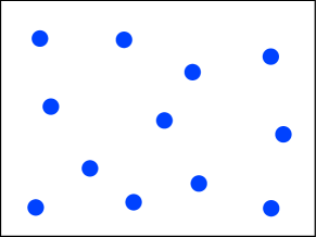
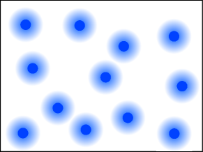
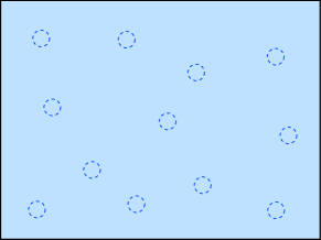
Figure 1: For purposes of illustration, this schematic shows diffusion spreadability at different times for the special case in which phase 2 is comprised of a spatial distribution of particles. The left panel depicts the uniform concentration of the solute species within phase 2 (dark blue regions) at time $t=0$. The middle panel depicts the spreading of diffusion information at short times. The right panel depicts the uniform concentration of the solute species throughout both phases (light blue region) in the infinite-time limit. The behavior of the spreadability ${\cal S}(t)$ as a function of time is intimately related to the underlying microstructure. Section V.2 describes remarkable links between the spreadability ${\cal S}(t)$, covering problem of discrete geometry, and nuclear magnetic resonance (NMR) measurements.

Remarkably, the consequences of Prager’s result are unknown because it has yet to be understood fundamentally or applied in any meaningful way. The purpose of this investigation is to explore the fundamental theoretical and practical implications of the spreadability ${\cal S}(t)$. We begin by generalizing Prager’s formula (1) to all space dimensions (Sec. III.1). We then obtain a new Fourier representation of the spreadability ${\cal S}(t)$ (Sec. III.2) in terms of the spectral density ${\tilde{\chi}_{{}_{V}}}({\bf k})$ (defined in Sec. II), which is obtainable from scattering experiments. There are many fundamental questions that we will explore. For example, what microstructural information is reflected by the spreadability ${\cal S}(t)$? What microstructures maximize spreadability up to time $t$? We determine microstructures for which the “spreadability” is “fast” or “slow,” thereby gaining an understanding of how the microstructure affects such time-dependent diffusion processes.

Using the exact direct- and Fourier-space representations of the spreadability (Sec. III), we derive closed-form general asymptotic expansions of the spreadability for any $d$ that apply at short times and long times in terms of crucial small- and large-scale microstructural information, respectively. We show that the small-time behavior of ${\cal S}(t)$ is determined by the derivatives of $S_{2}({\bf r})$ at the origin, the leading order term of order $t^{1/2}$ being proportional to the specific surface $s$ (interface area per unit volume). By contrast, the corresponding long-time behavior is determined by the form of the spectral density ${\tilde{\chi}_{{}_{V}}}({\bf k})$ at small wavenumbers.

We obtain exact results for ${\cal S}(t)$ for a variety of specific ordered and disordered model microstructures across dimensions that span from hyperuniform to antihyperuniform media (Secs. IV and V). Hyperuniform two-phase media are characterized by an anomalous suppression of volume-fraction fluctuations relative to garden-variety disordered media Zachary and Torquato (2009); Torquato (2018a) and can be endowed with novel physical properties Torquato (2018a); see Sec. II for precise mathematical definitions. For hyperuniform media, disordered or not, we show that the excess spreadability, ${\cal S}(\infty)-{\cal S}(t)$, decays to its long-time behavior exponentially faster than that of any non-hyperuniform two-phase medium, the ‘slowest” being antihyperuniform media (Sec. III.4). The stealthy hyperuniform class (see Sec. II) is characterized by an excess spreadability with the fastest decay rate among all hyperuniform media and hence all translationally invariant microstructures. Specifically, ${\cal S}(t)$ for stealthy hyperuniform media decays faster than any inverse power law (Sec. V), the latter of which applies to any nonstealthy disordered hyperuniform medium (Sec. III.4). Thus, the spreadability provides a new dynamic-based figure of merit to probe and classify the spectrum of possible microstructures that span between hyperuniform and nonhyperuniform media.

We establish that the microstructures with “fast” spreadabilities are also those that can be derived from efficient “coverings” of Euclidean space $\mathbb{R}^{d}$ (Sec. V.3). Moreover, in Sec. VI, we identify a heretofore unnoticed fascinating connection between the spreadability ${\cal S}(t)$ and noninvasive nuclear magnetic resonance (NMR) relaxation measurements in physical and biological porous media Brownstein and Tarr (1979); Mitra et al. (1992, 1993); Sen and Hürlimann (1994); Øren et al. (2002); Wedeen et al. (2005); Novikov et al. (2014). We close with concluding remarks (Sec. VII), including a “phase diagram” that schematically shows the spectrum of spreadability regimes and its relationship to the spectrum of microstructures.

II Background

II.1 Correlation Functions

A two-phase medium is fully statistically characterized by the $n$-point correlation functions Torquato (2002), defined by

$$S_{n}^{(i)}\left(\mathbf{x}_{1},...,\mathbf{x}_{n}\right)\equiv\left\langle{\cal I}^{(i)}(\mathbf{x}_{1})\ldots{\cal I}^{(i)}(\mathbf{x}_{n})\right\rangle,$$ (2)

where ${\cal I}^{(i)}({\bf x})$ is the indicator function for phase $i=1,2$, $n=1,2,3,\ldots$, and angular brackets denote an ensemble average. The function $S_{n}^{(i)}({\bf x}_{1},\ldots,{\bf x}_{n})$ also has a probabilistic interpretation, namely, it is the probability that the vertices of a polyhedron located at ${\bf x}_{1},\ldots,{\bf x}_{n}$ all lie in phase $i$. For statistically homogeneous media, $S_{n}^{(i)}\left(\mathbf{x}_{1},...,\mathbf{x}_{n}\right)$ is translationally invariant and hence depends only on the relative displacements of the points.

The autocovariance function $\chi_{{}_{V}}({\bf r})$, which is directly related to the two-point function $S_{2}^{(i)}({\bf r})$ and plays a central role in this paper, is defined by

$$\chi_{{}_{V}}({\bf r})\equiv S_{2}^{(1)}({\bf r})-\phi_{1}^{2}=S_{2}^{(2)}({\bf r})-\phi_{2}^{2}.$$ (3)

Here, we have assumed statistical homogeneity. At the extreme limits of its argument, $\chi_{{}_{V}}({\bf r})$ has the following asymptotic behavior: $\chi_{{}_{V}}({\bf r}=0)=\phi_{1}\phi_{2}$ and $\lim_{|{\bf r}|\rightarrow\infty}\chi_{{}_{V}}({\bf r})=0$ if the medium possesses no long-range order. If the medium is statistically homogeneous and isotropic, then the autocovariance function ${\chi_{{}_{V}}}({\bf r})$ depends only on the magnitude of its argument $r=|\bf r|$, and hence is a radial function. In such instances, its slope at the origin is directly related to the specific surface $s$, which is the interface area per unit volume. In particular, the well-known three-dimensional asymptotic result Debye et al. (1957) is easily obtained in any space dimension $d$:

$$\chi_{{}_{V}}({\bf r})=\phi_{1}\phi_{2}-\kappa(d)s\;|{\bf r}|+{\cal O}(|{\bf r}|^{2}),$$ (4)

where

$$\kappa(d)=\frac{\Gamma(d/2)}{2\sqrt{\pi}\Gamma((d+1)/2)}.$$ (5)

The nonnegative spectral density ${\tilde{\chi}}_{{}_{V}}({\bf k})$, which can be obtained from scattering experiments Debye and Bueche (1949); Debye et al. (1957), is the Fourier transform of $\chi_{{}_{V}}({\bf r})$ at wave vector $\bf k$, i.e.,

$${\tilde{\chi}}_{{}_{V}}({\bf k})=\int_{\mathbb{R}^{d}}\chi_{{}_{V}}({\bf r})e^{-i{\bf k\cdot r}}{\rm d}{\bf r}\geq 0,\qquad\mbox{for all}\;{\bf k}.$$ (6)

For isotropic media, the spectral density only depends on the wavenumber $k=|{\bf k}|$ and, as a consequence of (4), its decay in the large-$k$ limit is controlled by the exact following power-law form:

$${\tilde{\chi}}_{{}_{V}}({\bf k})\sim\frac{\gamma(d)\,s}{k^{d+1}},\qquad k\rightarrow\infty,$$ (7)

where

$$\gamma(d)=2^{d}\,\pi^{(d-1)/2}\,\Gamma((d+1)/2).$$ (8)

II.2 Hyperuniformity

The hyperuniformity concept generalizes the traditional notion of long-range order in many-particle systems to not only include all perfect crystals and perfect quasicrystals, but also exotic amorphous states of matter according to Torquato and Stillinger (2003); Torquato (2018a). For two-phase heterogeneous media in $d$-dimensional Euclidean space $\mathbb{R}^{d}$, which include cellular solids, composites, and porous media, hyperuniformity is defined by the following infinite-wavelength condition on the spectral density ${\tilde{\chi}}_{{}_{V}}({\bf k})$Zachary and Torquato (2009); Torquato (2018a), i.e.,

$$\lim_{|{\bf k}|\to 0}{\tilde{\chi}}_{{}_{V}}({\bf k})=0.$$ (9)

An equivalent definition of hyperuniformity is based on the local volume-fraction variance $\sigma^{2}_{{}_{V}}(R)$ associated with a $d$-dimensional spherical observation window of radius $R$. A two-phase medium in $\mathbb{R}^{d}$ is hyperuniform if its variance grows in the large-$R$ limit faster than $R^{d}$. This behavior is to be contrasted with those of typical disordered two-phase media for which the variance decays like the inverse of the volume $v_{1}(R)$ of the spherical observation window, which is given by

$$v_{1}(R)=\frac{\pi^{d/2}R^{d}}{\Gamma(1+d/2)}.$$ (10)

The hyperuniformity condition (9) dictates that the direct-space autocovariance function $\chi_{{}_{V}}({\bf r})$ exhibits both positive and negative correlations such that its volume integral over all space is exactly zero Torquato (2016), i.e.,

$$\int_{\mathbb{R}^{d}}\chi_{{}_{V}}({\bf r})d{\bf r}=0,$$ (11)

which is a direct-space sum rule for hyperuniformity.

II.3 Classification of Hyperuniform and Nonhyperuniform Media

The hyperuniformity concept has led to a unified means to classify equilibrium and nonequilibrium states of matter, whether hyperuniform or not, according to their large-scale fluctuation characteristics. In the case of hyperuniform two-phase media Zachary and Torquato (2009); Torquato (2018a), there are three different scaling regimes (classes) that describe the associated large-$R$ behaviors of the volume-fraction variance when the spectral density goes to zero as a power-law scaling ${\tilde{\chi}}_{{}_{V}}({\bf k})\sim|{\bf k}|^{\alpha}$ as $|\bf k|$ tends to zero:

$$\sigma^{2}_{{}_{V}}(R)\sim\begin{cases}R^{-(d+1)},\quad\quad\quad\alpha>1\qquad&\text{(Class I)}\\ R^{-(d+1)}\ln R,\quad\alpha=1\qquad&\text{(Class II)}\\ R^{-(d+\alpha)},\quad 0<\alpha<1\qquad&\text{(Class III).}\end{cases}$$ (12)

Classes I and III are the strongest and weakest forms of hyperuniformity, respectively. Class I media include all crystal structures, many quasicrystal structures and exotic disordered media Zachary and Torquato (2009); Torquato (2018a). Stealthy hyperuniform media are also of class I and are defined to be those that possess zero-scattering intensity for a set of wavevectors around the origin Torquato (2016), i.e.,

$${\tilde{\chi}}_{{}_{V}}({\bf k})=0\qquad\mbox{for}\;0\leq|{\bf k}|\leq K.$$ (13)

Examples of such media are periodic packings of spheres as well as unusual disordered sphere packings derived from stealthy point patterns Torquato (2016); Zhang et al. (2016).

By contrast, for any nonhyperuniform two-phase system, it is straightforward to show, using a similar analysis as for point configurations Torquato (2021), that the local variance has the following large-$R$ scaling behaviors:

$$\sigma^{2}_{{}_{V}}(R)\sim\begin{cases}R^{-d},&\alpha=0\quad\text{(typical nonhyperuniform)}\\ R^{-(d+\alpha)},&-d<\alpha<0\quad\text{(antihyperuniform)}.\\ \end{cases}$$ (14)

For a “typical” nonhyperuniform system, ${\tilde{\chi}}_{{}_{V}}(0)$ is bounded Torquato (2018a). In antihyperuniform systems, ${\tilde{\chi}}_{{}_{V}}(0)$ is unbounded, i.e.,

$$\lim_{|{\bf k}|\to 0}{\tilde{\chi}}_{{}_{V}}({\bf k})=+\infty,$$ (15)

and hence are diametrically opposite to hyperuniform systems. Antihyperuniform systems include systems at thermal critical points (e.g., liquid-vapor and magnetic critical points) Stanley (1987); Binney et al. (1992), fractals Mandelbrot (1982), disordered non-fractals Torquato et al. (2021), and certain substitution tilings Oğuz et al. (2019).

III Theory

III.1 Generalization of Prager’s formula for All Dimensions

Using the $d$-dimensional Green’s function for the time-dependent diffusion equation, it is straightforward to generalize Prager’s three-dimensional result for the spreadability ${\cal S}(t)$, given by (1), to any Euclidean space dimension $d$. After rearranging terms, we find that

$${\cal S}(t)=\frac{1}{(4\pi Dt)^{d/2}\,\phi_{2}}\int_{\mathbb{R}^{d}}[\phi_{2}-S_{2}({\bf r})]\exp[-r^{2}/(4Dt)]d{\bf r},$$ (16)

where it is to be noted that ${\cal S}(\infty)=\phi_{1}$, i.e., the infinite-time value of ${\cal S}(t)$. We note the identities

$$\frac{1}{(4\pi Dt)^{d/2}}\int_{\mathbb{R}^{d}}\exp[-r^{2}/(4Dt)]d{\bf r}=1$$ (17)

and

$$\frac{1}{(4\pi Dt)^{d/2}}\int_{\mathbb{R}^{d}}r^{2}\exp[-r^{2}/(4Dt)]d{\bf r}=2\,dD\,t.$$ (18)

The second identity is nothing more than the mean-square displacement of a freely diffusing particle in the long-time limit. Use of the first identity in (16) yields the difference ${\cal S}(\infty)-{\cal S}(t)$, which we call the excess spreadability, to be given by

$${\cal S}(\infty)-{\cal S}(t) = \frac{1}{(4\pi Dt)^{d/2}\,\phi_{2}}\int_{\mathbb{R}^{d}}\chi_{{}_{V}}({\bf r})\exp[-r^{2}/(4Dt)]d{\bf r}$$

$$= \frac{d\,\omega_{d}}{(4\pi Dt)^{d/2}\,\phi_{2}}\int_{0}^{\infty}r^{d-1}\chi_{{}_{V}}(r)\exp[-r^{2}/(4Dt)]dr,$$

where

$$\omega_{d}=\frac{\pi^{d/2}}{\Gamma(1+d/2)}$$ (20)

is the volume of a $d$-dimensional sphere of unit radius and $\chi_{{}_{V}}({\bf r})$ is the autocovariance function, defined by (3). In the second line of (LABEL:2), the autocovariance $\chi_{{}_{V}}(r)$ is the radial function that depends on the distance $r\equiv|{\bf r}|$, which results from averaging the vector-dependent quantity $\chi_{{}_{V}}({\bf r})$ over all angles, i.e.,

$$\chi_{{}_{V}}(r)=\frac{1}{\Omega}\int_{\Omega}\chi_{{}_{V}}({\bf r})\,d\Omega,$$ (21)

where $d\Omega$ is the differential solid angle and

$$\Omega=\frac{d\pi^{d/2}}{\Gamma(1+d/2)}$$ (22)

is the total solid angle contained in a $d$-dimensional sphere. It is important to stress that relation (LABEL:2) applies to all translationally invariant two-media, including periodic media.

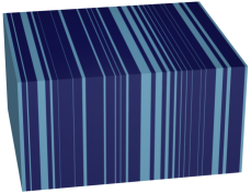
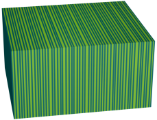
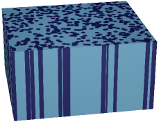
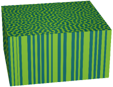
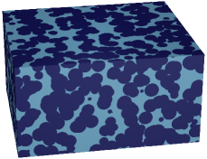
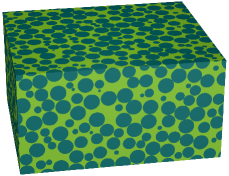
Figure 2: Models of nonhyperuniform and hyperuniform two-phase media with different symmetries are shown in blue (left) and green (right) colors, respectively. In each row, the spreadability is larger for the hyperuniform medium than that of the corresponding nonhyperuniform medium, as proved in Sec. III.4. Top row: 3D anisotropic stratified two-phase media consisting of infinite parallel slabs of phases 1 and 2 ($\phi_{2}=0.5$) whose thicknesses are derived from nonhyperuniform overlapping rods Torquato (2002) (left) and hyperuniform perturbed 1D integer lattice point patterns Klatt et al. (2020) (right). Formulas (LABEL:2) and (LABEL:3) with $d=1$ for ${\cal S}(t)$ apply rigorously for these 3D anisotropic structures. Middle row: 3D anisotropic two-phase media ($\phi_{2}=0.5$) with cylindrical symmetry obtained from nonhyperuniform oriented overlapping circular cylinders Torquato (2002) (left) and stealthy and hyperuniform oriented nonoverlapping circular cylinders Zhang et al. (2016); Torquato and Kim (2021) (right). Formulas (LABEL:2) and (LABEL:3) with $d=2$ for ${\cal S}(t)$ apply rigorously for these 3D anisotropic structures. Bottom row: 3D isotropic two-phase media ($\phi_{2}=0.636$) of overlapping spheres Torquato (2002) (left) and hyperuniform maximally random jammed spheres Klatt and Torquato (2014); Torquato (2018b) (right).

Figure 2 shows examples of three-dimensional (3D) nonhyperuniform and hyperuniform media with different symmetries for which formula (LABEL:2) for the spreadability rigorously applies. It is noteworthy that the formula (LABEL:2), as well as formula (LABEL:3) below, for one-dimensional (1D) cases (i.e., $d=1$) are also rigorously exact for the idealized three-dimensional (3D) statistically anisotropic stratified two-phase media of parallel slabs of phases 1 and 2, as illustrated in the top row of Fig. 2. This fact is easily proved by employing the first line of formula (LABEL:2), for example, with $d=3$ using Cartesian coordinates, and then recognizing that the vector-dependent quantity $\chi_{{}_{V}}({\bf r})$ is independent of the components of $\bf r$ in the directions orthogonal to the slab normal. Similarly, formulas (LABEL:2) and (LABEL:3) for two-dimensional (2D) cases (i.e., $d=2$) are rigorously exact for the idealized three-dimensional (3D) anisotropic media that possess transverse isotropy with respect to an axis of symmetry, as illustrated in the middle row of Fig. 2. The bottom row of Fig. 2 shows examples of 3D statistically isotropic disordered nonhyperuniform and hyperuniform media.

III.2 Fourier Representation of the Spreadability

Here, we obtain a Fourier representation of the spreadability, which is useful when scattering information is available. By Parseval’s theorem, the direct-space relation (LABEL:2) for the spreadability can be re-expressed in Fourier space as

$${\cal S}(\infty)-{\cal S}(t) = \frac{1}{(2\pi)^{d}\,\phi_{2}}\int_{\mathbb{R}^{d}}{\tilde{\chi}}_{{}_{V}}({\bf k})\exp[-k^{2}Dt]d{\bf k}$$

$$= \frac{d\,\omega_{d}}{(2\pi)^{d}\,\phi_{2}}\int_{0}^{\infty}k^{d-1}{\tilde{\chi}}(k)\exp[-k^{2}Dt]dk,$$

where ${\tilde{\chi}}_{{}_{V}}({\bf k})$ is the spectral density, which is the Fourier transform of $\chi_{{}_{V}}({\bf r})$, and $\bf k$ is the wave vector. In the second line of (LABEL:3), the spectral density ${\tilde{\chi}}_{{}_{V}}(k)$ is the radial function that depends on the wavenumber $k\equiv|{\bf k}|$, which results from averaging the vector-dependent quantity ${\tilde{\chi}}_{{}_{V}}({\bf k})$ over all angles, i.e.,

$${\tilde{\chi}}_{{}_{V}}(k)=\frac{1}{\Omega}\int_{\Omega}{\tilde{\chi}}_{{}_{V}}({\bf k})\,d\Omega,$$ (24)

$d\Omega$ is the differential solid angle. Now, since ${\tilde{\chi}}_{{}_{V}}({\bf k})$ is nonnegative for all $\bf k$, the integrand of (LABEL:3) is nonnegative and decreases with increasing $t$. Thus, the excess spreadability is a monotonically decreasing function of time and is itself nonnegative, i.e.,

$${\cal S}(\infty)-{\cal S}(t)\geq 0\qquad\mbox{for all}\;t$$ (25)

or, equivalently,

$${\cal S}(t)\leq\phi_{1}\qquad\mbox{for all}\;t.$$ (26)

In summary, we can ascertain the spreadability exactly for any microstructure across spatial dimensions using knowledge of the corresponding autocovariance via relation (LABEL:2) or the spectral density via (LABEL:3).

III.3 Small-Scale Structure via Short-Time Behavior of ${\cal S}(t)$

To obtain the short-time asymptotic behavior of ${\cal S}(t)$ for statistically homogeneous media, we recognize that the Gaussian term $\exp[-r^{2}/(4Dt)]$ in the direct-space representation of the spreadability (LABEL:2) is nonnegligibly small for short times for distances only near the spatial origin ($r=0$). Therefore, the short-time behavior of the integral in (LABEL:2) is determined by the small-$r$ expansion of $\chi_{{}_{V}}(r)$ about $r=0$:

$$\chi_{{}_{V}}(r)=\phi_{1}\phi_{2}-\frac{\omega_{d-1}}{\omega_{d}\,d}\,s\,r+\sum_{n=2}^{N}s_{n}r^{n},$$ (27)

where $s$ is the specific surface and the coefficient $s_{n}=(d^{n}\chi_{{}_{V}}(r)/dr^{n})_{r=0}$ is the $n$th order derivative at the origin. Substitution of (27) into (LABEL:2) yields the following exact asymptotic expansion of ${\cal S}(t)$ for any $d$:

$${\cal S}(t)=\frac{s}{\phi_{2}}\left(\frac{Dt}{\pi}\right)^{1/2}+\frac{d\,\omega_{d}}{\pi^{d/2}\phi_{2}}\sum_{n=2}^{N}2^{n-1}\,s_{n}\,\Gamma((n+d)/2)\,(Dt)^{n/2}\quad(t\to 0),$$ (28)

where we have employed the integral identity

$$\frac{1}{(4\pi Dt)^{d/2}} \int_{0}^{\infty}r^{m}\exp[-r^{2}/(4Dt)]dr$$

$$= 2^{m-d}\,{\pi^{-d/2}\Gamma((m+1)/2)}\,(Dt)^{(m+1-d)/2},$$

and $m$ is a nonnegative integer. It is noteworthy that if the upper limit $N$ in the sum (28) is infinite, i.e., the $s_{n}$ exist for all $n\geq 2$, formula (28) is an exact convergent series representation of the spreadability for all times. The first two terms of the short-time asymptotic expansion (28) are explicitly given by

$${\cal S}(t)=\frac{s}{\phi_{2}}\left(\frac{Dt}{\pi}\right)^{1/2}-\frac{2\,d\,s_{2}}{\phi_{2}}\,(Dt)+{\cal O}(Dt/a^{2})^{3/2},$$ (30)

where $a$ is some characteristic heterogeneity length scale. Note that the leading term is of order $t^{1/2}$, independent of the space dimension, and proportional to the specific surface $s$, which is intuitively clear, since the solute species is only just emerging from phase 2 in the immediate vicinity of the two-phase interface. The term of order $t$ is determined by the curvature of $\chi_{{}_{V}}(r)$ at the origin due to the presence of the coefficient $s_{2}$.

III.4 Large-Scale Structure via Long-Time Behavior of ${\cal S}(t)$

The long-time behavior of the spreadability ${\cal S}(t)$ is determined by the large-scale structural characteristics of the two-phase medium. Specifically, we see that the integrand of the Fourier representation (LABEL:3) of the spreadability is nonnegligibly small at long times for wavenumbers in the vicinity of the origin, i.e., the behavior of the spectral density ${\tilde{\chi}}_{{}_{V}}(k)$ in the infinite-wavelength limit. In the special situation in which ${\tilde{\chi}}_{{}_{V}}(k)$ is an analytic function at the origin, the spectral density admits a Taylor series expansion in only even powers of $k$ and whose coefficients depend on certain moments of the autocovariance function $\chi_{{}_{V}}(r)$, all of which must exist. Specifically, using (LABEL:3), we find the following exact series representation of the excess spreadability ${\cal S}(\infty)-{\cal S}(t)$:

$${\cal S}(\infty)-{\cal S}(t) = \frac{d\,\omega_{d}}{(4\pi Dt)^{d/2}\,\phi_{2}}\sum_{n=0}^{\infty}\frac{(-1)^{n}M_{2n+d-1}(\chi_{{}_{V}})}{n!(4Dt)^{n}},$$ (31)

where

$$M_{n}(\chi_{{}_{V}})=\int_{0}^{\infty}r^{n}\chi_{{}_{V}}(r)dr$$ (32)

is the $n$th moment of $\chi_{{}_{V}}(r)$. Observe now that truncation of the infinite series (31) yields the long-time asymptotic expansion of the excess spreadability. The first few terms of this asymptotic expansion are explicitly given by

$${\cal S}(\infty)-{\cal S}(t) = \frac{d\,\omega_{d}}{(4\pi Dt)^{d/2}\,\phi_{2}}\left[M_{d-1}(\chi_{{}_{V}})-\frac{M_{d+1}(\chi_{{}_{V}})}{4Dt}+\frac{M_{d+3}(\chi_{{}_{V}})}{32(Dt)^{2}}-\cdots\right]\quad(t\to\infty).$$ (33)

Note that since the moment $M_{d-1}(\chi_{{}_{V}})$ is nonnegative, then the leading-order term of the sum is of order $t^{-d/2}$ whenever the system is nonhyperuniform, i.e., $M_{d-1}(\chi_{{}_{V}})$ does not vanish, and all moments exist.

Now we recognize that if this type of two-phase media is hyperuniform, then $M_{d-1}(\chi_{{}_{V}})$ in (33) vanishes, implying that the leading-order term of the sum that involves the moment $M_{d+1}(\chi_{{}_{V}})$ is of order $t^{-(d+2)/2}$, i.e.,

$${\cal S}(\infty)-{\cal S}(t) = \frac{d\,\omega_{d}}{4(4\pi)^{d/2}(Dt)^{d/2+1}\,\phi_{2}}\left[-M_{d+1}(\chi_{{}_{V}})+\frac{M_{d+3}(\chi_{{}_{V}})}{8Dt}+\cdots\right]\quad(t\to\infty).$$ (34)

In light of the nonnegativity condition (25), the moment $M_{d+1}(\chi_{{}_{V}})$ must be negative for a hyperuniform medium. Moreover, since the spectral density ${\tilde{\chi}}_{{}_{V}}(k)$ is analytic at $k=0$ [i.e, all moments of $\chi_{{}_{V}}(r)$ exist], then it follows that ${\tilde{\chi}}_{{}_{V}}(k)\propto-M_{d+1}(\chi_{{}_{V}})k^{2}$ in the limit $k\to 0$, and hence the two-phase medium is hyperuniform of class I. Thus, we see that for such hyperuniform media, disordered or not, ${\cal S}(\infty)-{\cal S}(t)$ decays to its long-time behavior exponentially faster than that of any non-hyperuniform two-phase medium.

Now we consider the more general class of two-phase media in which the spectral density may be a nonanalytic function at the origin such that it obeys the following power-law scaling in the infinite-wavelength limit:

$$\lim_{|{\bf k}|\to{\bf 0}}{\tilde{\chi}}_{{}_{V}}({\bf k})=B|{\bf k}a|^{\alpha},$$ (35)

where $B$ is a positive dimensionless constant, $\alpha$ is an exponent that lies in the interval $(-d,\infty)$, and $a$ represents some characteristic heterogeneity length scale. Antihyperuniform media constitute cases in which $-d<\alpha<0$. The case $\alpha=0$ corresponds to nonhyperuniform media, while the cases $\alpha>0$ correspond to hyperuniform media that may belong to class I, II or III (see Sec. II.3). This small-wavenumber behavior enables us to determine the more general long-time asymptotic behavior of ${\cal S}(t)$ using the Fourier representation (LABEL:3). Specifically, we find the following general asymptotic expansion:

$${\cal S}(\infty)-{\cal S}(t)=\frac{B\,\Gamma((d+\alpha)/2)\,\phi_{2}}{2^{d}\,{\pi}^{d/2}\,\Gamma(d/2)\,(Dt/a^{2})^{(d+\alpha)/2}}+{o}\left((Dt/a^{2})^{-(d+\alpha)/2}\right)\quad(Dt/a^{2}\gg 1),$$ (36)

where ${o}(x)$ signifies all terms of order less than $x$. Thus, we see that the long-time asymptotic behavior of ${\cal S}(t)$ is determined by the exponent $\alpha$ and the space dimension $d$, i.e., at long times, ${\cal S}(t)$ approaches the value $\phi_{1}$ with a power-law decay $1/t^{(d+\alpha)/2}$, implying a faster decay as $\alpha$ increases for some dimension $d$. When $\alpha$ is bounded and positive, this result means that class I hyperuniform media has the fastest decay, followed by class II and then class III, which has the slowest decay among hyperuniform media. Of course, antihyperuniform media with $\alpha\to-d$ has the slowest decay among all translationally invariant media. In the stealthy limit in which $\alpha\to\infty$, the predicted infinitely-fast inverse-power decay rate implies that the infinite-time aysmptote is approached exponentially fast. This result will be demonstrated explicitly in the case of periodic media, which are stealthy, as well as disordered stealthy hyperuniform media.

IV Applications to Nonhyperuniform, Hyperuniform and Antihyperuniform Media

IV.1 Standard Nonhyperuniform Media

It is instructive to first consider the spreadability ${\cal S}(t)$ for models of typical nonhyperuniform two-phase media. Prototypical examples are Debye random media Yeong and Torquato (1998), which are defined entirely by the following monotonic radial autocovariance function:

$$\chi_{{}_{V}}(r)=\phi_{1}\phi_{2}\exp(-r/a).$$ (37)

Such media can never be hyperuniform because the sum rule (11) requires both positive and negative correlations Torquato (2016). Debye et al. Debye et al. (1957) hypothesized the simple exponential form (37) to model three-dimensional media with phases of “fully random shape, size, and distribution.” It was many years after their 1957 study that such autocovariance functions were shown to be realizable in two Yeong and Torquato (1998); Chiu et al. (2013); Ma and Torquato (2020) and three Jiao et al. (2007); Torquato (2020) dimensions. The corresponding spectral density is given by

$${\tilde{\chi}}_{{}_{V}}(k)=\frac{\phi_{1}\phi_{2}\,2^{d}\,\pi^{d-1}\,a^{d}}{\omega_{d-1}\,[1+(ka)^{2}]^{(d+1)/2}}.$$ (38)

Therefore, for small wavenumbers,

$${\tilde{\chi}}_{{}_{V}}(k)=\phi_{1}\phi_{2}\frac{2^{d}\pi^{d-1}\,a^{d}}{\omega_{d-1}}[1-\frac{(d+1)}{2}(ka)^{2}+{\cal O}((ka)^{4})]$$ (39)

so that ${\tilde{\chi}}_{{}_{V}}(0)=\phi_{1}\phi_{2}2^{d}\pi^{d-1}\,a^{d}/\omega_{d-1}$. The spectral density is plotted in Fig. 3 for the first three space dimensions. We observe that Debye random media departs from hyperuniformity superexponentially fast as the space dimension increases; specifically, ${\tilde{\chi}}_{{}_{V}}(0)/(\phi_{1}\phi_{2}a^{d})\sim\sqrt{2}[2\pi d/\exp(1)]^{d/2}$ for large $d$.

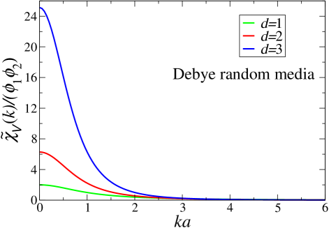
Figure 3: The scaled spectral density ${\tilde{\chi}}_{{}_{V}}(k)/(\phi_{1}\phi_{2})$ versus wavenumber $k$ for Debye random media for the first three space dimensions, as obtained from (38).

It is convenient to rewrite the direct-space representation of the spreadability ${\cal S}(t)$, given by (LABEL:2), as follows:

$${\cal S}(\infty)-{\cal S}(t)=\frac{d\omega_{d}\phi_{1}}{(4\pi Dt/a^{2})^{d/2}}I_{d}(t),$$ (40)

where

$$I_{d}(t)=\frac{1}{a^{d}}\int_{0}^{\infty}r^{d-1}\exp(-r/a)\exp[-r^{2}/(4Dt)]dr.$$ (41)

We can obtain a closed-form exact expression for ${\cal S}(t)$ for Debye random media for any $d$ using the recurrence relation

$$I_{d+2}(t)=\frac{2Dt}{a^{2}}\left[d\,I_{d}-I_{d+1}\right].$$ (42)

Specifically, the explicit expressions

$$I_{1}(t)=\exp(Dt/a^{2})\,\sqrt{\pi Dt/a^{2}}\,\left[1-\mbox{erf}(\sqrt{Dt/a^{2}})\right]$$ (43)

and

$$I_{2}(t)=\frac{2Dt}{a^{2}}\left\{1-\exp(Dt/a^{2})\,\sqrt{\pi Dt/a^{2}}\,\left[1-\mbox{erf}(\sqrt{Dt/a^{2}})\right]\right\},$$ (44)

for the first two dimensions combined with the recurrence relation (42) enables one to obtain $I_{d}$ for any $d\geq 3$. For example, for $d=3$, we have

$$I_{3}(t)=\frac{2Dt}{a^{2}}\Big{\{}\exp(Dt/a^{2})\,\sqrt{\pi Dt/a^{2}}\,\left[1-\mbox{erf}(\sqrt{Dt/a^{2}})\right]\left[1+2Dt/a^{2}\right]-2Dt/a^{2}\Big{\}}.$$ (45)

We also note that the $n$th moment of the autocovariance of Debye random media for any $d$ is given by

$$M_{n}(\chi_{{}_{V}})=\phi_{1}\phi_{2}\,n!\,a^{n+1}.$$ (46)

This result enables us to obtain another exact representation of the spreadability via the infinite series (31).

For any space dimension $d$, the short-time behavior of the ${\cal S}(t)$ is given by

$${\cal S}(t)=\frac{s}{\phi_{2}}\left(\frac{Dt/a^{2}}{\pi}\right)^{1/2}-\frac{d}{\phi_{2}}\left(\frac{Dt}{a^{2}}\right)+{\cal O}((Dt/a^{2})^{3/2}),$$ (47)

where

$$s=\frac{\phi_{1}\phi_{2}\omega_{d}d}{\omega_{d-1}\,a}$$ (48)

is the specific surface for a Debye random medium and we have used (30). Employing (31) and (46), we see that the first two terms of the long-time asymptotic expansion of the spreadability are given by

$${\cal S}(\infty)-{\cal S}(t)=\frac{(d-1)!\,d\omega_{d}\phi_{2}}{(4\pi Dt/a^{2})^{d/2}}-\frac{(d+1)!\,d\omega_{d}\phi_{2}}{(4\pi Dt/a^{2})^{(d+2)/2}}+{\cal O}\left((Dt/a^{2})^{-(d+4)/2}\right).$$ (49)

Figure 4 shows the small- and intermediate-time behaviors of the spreadability for Debye random media in the first three space dimensions. It is seen that the effect of increasing dimensionality is to increase the spreadability for a fixed time for almost all times, namely, for dimensionless times $Dt/a^{2}>1$.

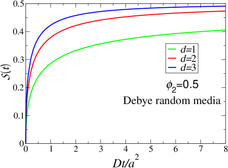
Figure 4: The spreadability ${\cal S}(t)$ versus dimensionless time $Dt/a^{2}$ for small to intermediate times for Debye random media in the first three space dimensions.

IV.2 Disordered Hyperuniform Media

To model hyperuniform two-phase media in $\mathbb{R}^{d}$, Torquato Torquato (2016) considered the following family of autocovariance functions:

$$\frac{\chi_{{}_{V}}(r)}{\phi_{1}\phi_{2}}=c\,e^{-r/a}\cos(qr+\theta),$$ (50)

where the parameters $q$ and $\theta$ are the wavenumber and phase associated with the oscillations of $\chi_{{}_{V}}(r)$, respectively, $a$ is a correlation length and $c$ is a normalization constant to be chosen so that the right-hand side of (50) is unity for $r=0$. In the special case in which $\theta=0$ and $c=1$, Torquato showed that the corresponding autocovariance function satisfies all of the necessary realizability conditions and hyperuniformity constraint (11) for $d=2$ if $(qa)^{2}=1$ and for $d=3$ if $(qa)^{2}=1/3$. Thus, the spectral densities for $d=2$ and $d=3$ are respectively given by

$$\frac{{\tilde{\chi}}_{{}_{V}}(k)}{\phi_{1}\phi_{2}}=\frac{2\pi(ka)^{2}[A(k)+B(k)]+4\pi[A(k)-B(k)]\,a^{2}}{[(ka)^{4}+4][A^{2}(k)+B^{2}(k)]},$$ (51)

and

$$\frac{{\tilde{\chi}}_{{}_{V}}(k)}{\phi_{1}\phi_{2}}=\frac{216\pi\,[3(ka)^{2}+8](ka)^{2}\,a^{3}}{81(ka)^{8}+216(ka)^{6}+432(ka)^{4}+384(ka)^{2}+256},$$ (52)

where

$$A(k)=\sqrt{(ka)^{2}/2+\sqrt{(ka)^{4}+4}/2},\qquad B(k)=A^{-1}(k).$$ (53)

It was shown that for the special case $\theta=0$ and $d=1$, the function (50) does not satisfy the hyperuniformity constraint for any values of the parameters $q$ and $\theta$. However, we note here that (50) meets all of the known realizability conditions and the hyperuniformity constraint for $d=1$, provided that the phase is given by $\theta=\tan^{-1}\left(1/(qa)\right)$, implying that the normalization constant is $c=[1+(qa)^{2}]^{1/2}/(qa)$. For concreteness, we set $qa=1$, and hence $c=2$ and $\theta=\pi/4$. Taking the Fourier transform of (50) with these parameters yields the spectral density to be given by

$$\frac{{\tilde{\chi}}_{{}_{V}}(k)}{\phi_{1}\phi_{2}}=\frac{4\,(ka)^{2}\,a}{(ka)^{4}+4}.$$ (54)

Substitution of this expression into (LABEL:3) yields the following exact formula for the spreadability

$${\cal S}(\infty)-{\cal S}(t)=\frac{4\phi_{1}\,\sqrt{t}}{\sqrt{\pi}}[s_{1,1/2}(2t)-1],$$ (55)

where $s_{\mu,\nu}(x)$ is the Lommel function of the second kind Abramowitz and Stegun (1972).

Figure 5 depicts the scaled spectral densities for the aforementioned disordered hyperuniform models in the first three space dimensions. It is seen that the peak values increase substantially with increasing dimension.

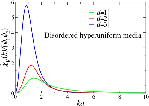
Figure 5: The scaled spectral density ${\tilde{\chi}}_{{}_{V}}(k)/(\phi_{1}\phi_{2})$ versus wavenumber $k$ for disordered hyperuniform media for the first three space dimensions, as obtained from relations (51), (52) and (54).

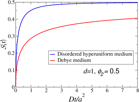
Figure 6: Comparison of the spreadabilities for Debye random media and disordered hyperuniform media for $d=1$ and $\phi_{2}=0.5$.

The $n$th moment $M_{n}(\chi_{{}_{V}})$ of the autocovariance function (50) for any $n$ is given exactly by

$$M_{n}(\chi_{{}_{V}})=c\phi_{1}\phi_{2}\frac{n!a^{n+1}}{[1+(qa)^{2}]^{n+1}}\left[\cos(\beta)\cos(\theta)-\sin(\beta)\sin(\theta)\right],$$ (56)

where $\beta=(n+1)\arctan(qa)$. The specific expressions for the moments for the parameters used above for the first three space dimensions are given in Appendix A, which yield corresponding exact representations of the spreadability ${\cal S}(t)$ via the infinite series (31). Using these results and (34) yields the corresponding long-time asymptotic expansions of ${\cal S}(t)$ for the first three space dimensions:

$${\cal S}(\infty)-{\cal S}(t)=\frac{\phi_{1}}{4\sqrt{\pi}\,(Dt/a)^{3/2}}+{\cal O}\left((Dt/a)^{-5/2}\right)\quad(d=1),$$ (57)

$${\cal S}(\infty)-{\cal S}(t)=\frac{3\phi_{1}}{16\,(Dt/a)^{2}}+{\cal O}\left((Dt/a)^{-3}\right)\quad(d=2),$$ (58)

and

$${\cal S}(\infty)-{\cal S}(t)=\frac{81\phi_{1}}{64\,\sqrt{\pi}(Dt/a)^{5/2}}+{\cal O}\left((Dt/a)^{-7/2}\right)\quad(d=3).$$ (59)

For fixed dimension, we have already noted that the spreadability for disordered hyperuniform media will be substantially larger than that of nonhyperuniform media. Figure 6 specifically demonstrates this distinction in one dimension by comparing the spreadabilities for Debye random media and disordered hyperuniform media.

IV.3 Antihyperuniform Media

As a model of antihyperuniform media in three dimensions, we consider here the following autocovariance function

$$\frac{\chi_{{}_{V}}(r)}{\phi_{1}\phi_{2}}=\frac{1}{1+2(r/a)+(r/a)^{2}}.$$ (60)

This monotonic functional form meets all of the known necessary realizability conditions on a valid autocovariance function Torquato (2016). It is clear that any $n$th order moment $M_{n}(\chi_{{}_{V}})$ for $n\geq 1$ is unbounded. The corresponding spectral density is given by

$${\tilde{\chi}}_{{}_{V}}(k)=\frac{4\pi a^{2}}{ka}\Big{[}\mbox{Ci}(ka)[ka\cos(ka)+\sin(ka)]+\mbox{Ssi}(ka)[ka\sin(ka)-\cos(ka)\Big{]},$$ (61)

where $\mbox{Ci}(x)\equiv\int_{0}^{x}dt\cos(t)/t$ is the cosine integral, $\mbox{Ssi}(x)\equiv\mbox{Si}(x)-\pi/2$ is the shifted sine integral and $\mbox{Si}(x)\equiv\int_{0}^{x}dt\sin(t)/t$ is the sine integral. We see that ${\tilde{\chi}}_{{}_{V}}(k)\sim 2\pi^{2}/k$ in the limit $k\to 0$, which is consistent with the power-law decay $1/r^{2}$ of the $\chi_{{}_{V}}(r)$ in the limit $r\to\infty$. The spectral density is plotted in Fig. 7.

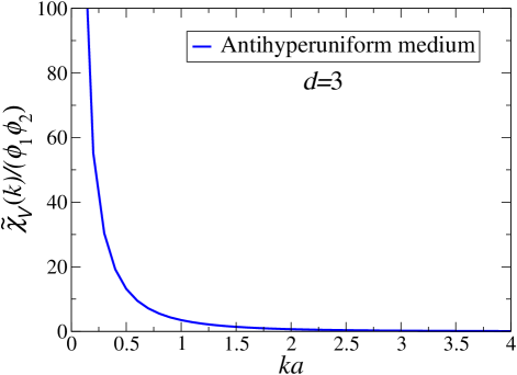
Figure 7: The scaled spectral density ${\tilde{\chi}}_{{}_{V}}(k)/(\phi_{1}\phi_{2})$ versus wavenumber $k$ for antihyperuniform media in three dimensions, as obtained from (61).

We have already observed that the excess spreadability for antihyperuniform media will have the slowest decay to its infinite-time behavior relative to that of disordered hyperuniform media or even to nonhyperuniform media in which the spectral density is bounded at the origin. These distinguished behaviors are clearly exhibited in Figure 6 where the excess spreadabilities are compared for these three different cases in three dimensions. The long-time inverse power-law scalings of ${\cal S}(\infty)-{\cal S}(t)$ for the hyperuniform, nonhyperuniform and antihyperuniform three-dimensional models are $1/t^{5/2}$, $1/t^{3/2}$ and $1/t$, respectively, as obtained from (36).

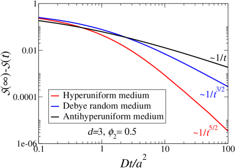
Figure 8: Comparison of the excess spreadabilities for Debye random media, disordered hyperuniform media and antihyperuniform media for $d=3$ and $\phi_{2}=0.5$. The long-time inverse power-law scalings of ${\cal S}(\infty)-{\cal S}(t)$ for each of these models is indicated.

V Applications to Stealthy Hyperuniform Media

In Sec. III.4, we indicated that that the infinite-time aysmptotes of the spreadability of stealthy hyperuniform media are approached exponentially fast and hence faster than any inverse power-law, which applies to nonhyperuniform and nonstealthy hyperuniform media. In this section, we explicitly demonstrate such long-time behaviors of both stealthy disordered and ordered media. We also describe how the speadability of stealthy hyperuniform media is linked to the covering problem of discrete geometry Conway and Sloane (1998); Torquato (2010).

V.1 Disordered Stealthy Hyperuniform Sphere Packings

Consider a packing of identical spheres of radius $a$, which we take to be phase 2. The packing fraction is $\phi_{2}=\rho v_{1}(a)$, where $\rho$ is the number density and $v_{1}(a)$ is the volume of a sphere [cf. (10)]. The spectral density of such a packing, hyperuniform or not, can be expressed in terms of the structure factor $S({\bf k})$ according to Torquato and Stell (1985); Torquato (2002, 2016)

$${\tilde{\chi}}_{{}_{V}}({\bf k}){\tilde{\chi}}({\bf k}) = \rho\,{\tilde{m}}^{2}(k;a)S({\bf k})$$ (62)

$$= \phi_{2}\,{\tilde{\alpha}}_{2}(k;a)S({\bf k})$$

where ${\tilde{m}}(k;a)$ is the Fourier transform of the sphere indicator function,

$${\tilde{\alpha}}(ka) = \frac{1}{v_{1}(a)}{\tilde{m}}^{2}(k;a)$$ (63)

$$= \frac{1}{v_{1}(a)}\left(\frac{2\pi a}{k}\right)^{d}J_{d/2}^{2}(ka)$$

$$= 2^{d}\pi^{d/2}\Gamma(d/2+1)\frac{J_{d/2}^{2}(ka)}{k^{d}}.$$

$${\tilde{\alpha}}_{2}(k;a)=2^{d}\pi^{d/2}\Gamma(d/2+1)\frac{J_{d/2}^{2}(ka)}{k^{d}}$$ (64)

is the Fourier transform of the scaled intersection volume of two spherical windows Torquato and Stillinger (2003). The zero-$k$ and large-$k$ of this function are given respectively by

$${\tilde{\alpha}}_{2}(0;a)=v_{1}(a)$$ (65)

and

$${\tilde{\alpha}}_{2}(k;a)\sim 2^{d+1}\pi^{d/2-1}\Gamma(1+d/2)\frac{\cos^{2}[ka-(d+1)/4]}{ak^{d+1}}\quad(ka\to\infty).$$ (66)

Moreover, we have the following integral condition:

$$\frac{1}{(2\pi)^{d}}\int_{\mathbb{R}^{d}}{\tilde{\alpha}}_{2}(k;a)d{\bf k}=1.$$ (67)

If the point configuration specified by the sphere centers is hyperuniform, then $\lim_{|{\bf k}|\to 0}S({\bf k})=0$, and hence the dispersion or packing is hyperuniform, since it immediately follows from (62) that the stealthy hyperuniformity condition (9) on the spectral density is obeyed. Moreover, if the sphere centers constitute a stealthy and hyperuniform point configuration, $S({\bf k})=0$ for $0\leq|{\bf k}|\leq K$, and hence it follows that the spectral density is also identically zero up to the cut-off value $K$, i.e., it obeys relation (13).

Disordered stealthy hyperuniform packings have been generated using the collective-coordinate optimization procedure Torquato et al. (2015) by decorating the resulting ground-state point configurations by nonoverlapping spheres Zhang et al. (2016); Kim and Torquato (2020). The degree of order of such ground states depends on a tuning parameter $\chi$, which measures the extent to which the ground states are constrained by the size of the cut-off value $K$ relative to the number of degrees of freedom. For $\chi<1/2$, the ground states are typically disordered and uncountably infinitely degenerate in the infinite-volume limit Torquato et al. (2015). Using the fact that $\rho\chi=v_{1}(K)/[2d(2\pi)^{d}]$ Torquato et al. (2015), it immediately follows that for identical nonoverlapping spheres of radius $a$ that the dimensionless stealthy cut-off value $Ka$ in terms of the packing fraction $\phi_{2}$ for any space dimension $d$ is given by

$$(Ka)^{d}=d2^{d+1}\Gamma^{2}(1+d/2)\phi_{2}\chi.$$ (68)

Given the specific stealthy form obtained from (62), one can compute the spreadability from formula (LABEL:3). Our main interest here is to determine from this formula the exact long-time asymptotic form for disordered stealthy packings. Noting that at long times, the spectral density can be replaced with its constant value at $k=K$, we find

$${\cal S}(\infty)-{\cal S}(t)\sim\frac{d\omega_{d}}{(2\pi)^{d}}{\tilde{\alpha}}_{2}(Ka)S(K)\int_{K}^{\infty}k^{d-1}\exp(-k^{2}Dt)dk=\frac{d\omega_{d}}{2(2\pi)^{d}}{\tilde{\alpha}}_{2}(Ka)S(K)\frac{\exp(-K^{2}Dt)}{K^{2}Dt}\;(Dt/a^{2}\gg 1).$$ (69)

We see that the decay of the excess spreadability of a disordered stealthy hyperuniform two-phase medium is exponentially faster than that of any class I hyperuniform system in which the exponent $\alpha>1$, specified by (35), is bounded.

V.2 Ordered Stealthy Hyperuniform Sphere Packings

It is instructive to compare and contrast the spreadability of disordered stealthy hyperuniform packings to that of their ordered stealthy hyperuniform counterparts. For this purpose, we consider identical nonverlapping spheres of radius $a$ centered on the sites of a periodic lattice, which are stealthy and hyperuniform up to the first Bragg peak Torquato et al. (2015). We begin by noting that the structure factor of the sites of a Bravais lattice in $\mathbb{R}^{d}$, excluding forward scattering, is given by

$$S({\bf k})=\frac{(2\pi)^{d}}{v_{c}}\sum_{{\bf Q}\neq{\bf 0}}\delta({\bf k}-{\bf Q}),$$ (70)

where $v_{c}$ is the volume of a fundamental cell in direct space and $\bf Q$ denotes a reciprocal lattice (Bragg) vector. Substitution of (62) and (70) into (LABEL:3) yields

$${\cal S}(\infty)-{\cal S}(t)=\phi_{2}\sum_{{\bf Q}\neq{\bf 0}}\frac{{\tilde{\alpha}}_{2}(|{\bf Q}|a)}{v_{1}(a)}\exp[-|{\bf Q}|^{2}Dt].$$ (71)

Alternatively, we can recast this equation by employing the angular-averaged structure factor $S(k)$, which is given by

$$S(k)=\frac{(2\pi)^{d}}{v_{c}}\sum_{n=1}\frac{Z(Q_{n})}{s_{1}(Q_{n})}\delta(k-Q_{n}),$$ (72)

where $Z(Q_{n})$ is the coordination number at radial distance $Q_{n}$, $s_{1}(R)=d\pi^{d/2}R^{d-1}/\Gamma(1+d/2)$ is the surface area of $d$-dimensional sphere of radius $R$, and $\delta(k)$ is a radial Dirac-delta function.

Table 1: The scaled first Bragg peak $Q_{1}a$ for one-dimensional periodic packings of spheres (rods) of radius $a$ derived from common crystal structures in terms of the packing fraction $\phi_{2}$. The corresponding maximal packing fraction $\phi_{2}^{max}$ for each structure is also listed. In the case of a periodic packing with a an $n$-particle basis, $\eta$ is the dimensionless length of the fundamental cell in terms of the minimal nearest-neighbor distance and hence the maximal packing fraction $n/\eta$ is always less than or equal to unity. The packing with the largest value of $Q_{1}a$ is the one derived from the integer lattice $\mathbb{Z}$.

Crystal Structure	$Q_{1}a$	$\phi_{2}^{max}$
Integer lattice ($\mathbb{Z}$)	$\pi\phi_{2}$	1
Periodic with $n$-particle basis	$\pi\phi_{2}/n$	$n/\eta$

Table 2: The scaled first Bragg peak $Q_{1}a$ (raised to the power 2) for two-dimensional periodic packings of spheres (circular disks) of radius $a$ derived from common crystal structures in terms of the packing fraction $\phi_{2}$. The corresponding maximal packing fraction $\phi_{2}^{max}$ for each structure is also listed. The packing with the largest value of $Q_{1}a$ is the one derived from the triangular lattice $A_{2}\equiv A_{2}^{*}$.

Crystal Structure	$(Q_{1}a)^{2}$	$\phi_{2}^{max}$
Triangular lattice ($A_{2}\equiv A_{2}^{*}$)	$(8\pi/\sqrt{3})\phi_{2}=(14.5103\ldots)\phi_{2}$	$\pi/\sqrt{12}=0.9068\ldots$
Square lattice ($\mathbb{Z}^{2}=\mathbb{Z}^{2}_{*}$)	$(4\pi)\phi_{2}=(12.5663\ldots)\phi_{2}$	$\pi/4=0.7853\ldots$
Honeycomb crystal ($\mbox{Dia}_{2}$)	$(4\pi/\sqrt{3})\phi_{2}=(7.2551\ldots)\phi_{2}$	$\pi/(3\sqrt{3})=0.6045\ldots$
Kagomé crystal ($\mbox{Kag}_{2}$)	$[8\pi/(3\sqrt{3})]\phi_{2}=4.8367\ldots)\phi_{2}$	$3\pi/(8\sqrt{3})=0.6801\ldots$

Table 3: The scaled first Bragg peak $Q_{1}a$ (raised to the power 3) for three-dimensional periodic packings of spheres of radius $a$ derived from common crystal structures in terms of the packing fraction $\phi_{2}$. The corresponding maximal packing fraction $\phi_{2}^{max}$ for each structure is also listed. The packing with the largest value of $Q_{1}a$ is the one derived from the BCC lattice $D_{3}^{*}$.

Crystal Structure	$(Q_{1}a)^{3}$	$\phi_{2}^{max}$
BCC lattice ($D_{3}^{*}$)	$(6\sqrt{2}\pi^{2})\phi_{2}=(83.7463\ldots)\phi_{2}$	$\sqrt{3}\pi/8=0.6801\ldots$
FCC lattice ($D_{3}\equiv A_{3}$)	$(9\sqrt{3}\pi^{2}/2)\phi_{2}=(76.9259\ldots)\phi_{2}$	$\pi/\sqrt{18}=0.7408\ldots$
HCP crystal	$(8\sqrt{6}\pi^{2}/3)\phi_{2}=(64.4679\ldots)\phi_{2}$	$\pi/\sqrt{18}=0.7408\ldots$
SC lattice ($Z_{3}\equiv Z_{3}^{*}$)	$6\pi^{2}\phi_{2}=(59.2176\ldots)\phi_{2}$	$\pi/6=0.5235\ldots$
Simple hexagonal lattice	$3\sqrt{3}\pi^{2}\phi_{2}=(51.2839\ldots)\phi_{2}$	$\pi/(3\sqrt{3})=0.6045\ldots$
Diamond crystal ($\mbox{Dia}_{3}$)	$(9\sqrt{3}\pi^{2}/4)\phi_{2}=(38.4629\ldots)\phi_{2}$	$\sqrt{3}\pi/16=0.3400\ldots$
Pyrochlore crystal ($\mbox{Kag}_{3}$)	$(9\sqrt{3}\pi^{2}/8)\phi_{2}=(19.2314\ldots)\phi_{2}$	$\sqrt{2}\pi/12=0.3702\ldots$

Table 4: The scaled first Bragg peak $Q_{1}a$ (raised to the power 4) for four-dimensional periodic packings of spheres of radius $a$ derived from common crystal structures in terms of the packing fraction $\phi_{2}$. The corresponding maximal packing fraction $\phi_{2}^{max}$ for each structure is also listed. The packing with the largest value of $Q_{1}a$ is the one derived from the four-dimensional checkerboard lattice $D_{4}\equiv D_{4}^{*}$.

Crystal Structure	$(Q_{1}a)^{4}$	$\phi_{2}^{max}$
$D_{4}$ lattice	$64\pi^{2}\phi_{2}$	$\pi^{2}/16=0.6168\ldots$
$\mathbb{Z}^{4}$ lattice	$32\pi^{2}\phi_{2}$	$\pi^{2}/16=0.3084\ldots$
$\mbox{Dia}_{4}$ crystal	$32\pi^{2}\phi_{2}$	$\sqrt{5}\pi^{2}/125=0.1765\ldots$
$\mbox{Kag}_{4}$ crystal	$(64\pi^{2}/5)\phi_{2}$	$\sqrt{5}\pi^{2}/128=0.1724\ldots$

Now we recognize that expression (72) for $S(k)$ applies more generally to periodic packings in which there are $N$ particles per fundamental cell, provided that $Z(Q_{n})$ is interpreted to be the expected coordination number at radial distance $Q_{n}$. Thus, for periodic packings, we have

$${\cal S}(\infty)-{\cal S}(t)=\phi_{2}\sum_{n=1}Z(Q_{n})\frac{{\tilde{\alpha}}_{2}(Q_{n}\,a)}{v_{1}(a)}\exp[-Q_{n}^{2}Dt],$$ (73)

where the packing fraction is given by

$$\phi_{2}=\frac{Nv_{1}(a)}{v_{c}}.$$ (74)

At large times, the first term in the sum of (73) is the dominant contribution and so

$${\cal S}(\infty)-{\cal S}(t)\sim\frac{\phi_{2}Z(Q_{1})\,{\tilde{\alpha}}_{2}(Q_{1}\,a)}{v_{1}(a)}\exp[-Q_{1}^{2}Dt]\qquad(Dt/a^{2}\gg 1),$$ (75)

where $Q_{1}$ is the first (smallest positive) Bragg wavenumber. Result (75), which is also a lower bound for all times, means that among all periodic packings of identical spheres in $\mathbb{R}^{d}$ at a fixed packing fraction $\phi_{2}$, the one with the largest first Bragg peak will have the fastest approach to the infinite-time behavior in space dimension $d$. In dimensions one, two, three and four, these optimal packings for the spreadability correspond to the integer lattice $\mathbb{Z}$, triangular lattice $A_{2}$, body-centered cubic (BCC) lattice $D_{3}^{*}$ (dual to the face-centered cubic (FCC) or checkerboard lattice $D_{3}$), and the four-dimensional checkerboard lattice $D_{4}$ Torquato et al. (2015), respectively. Tables I-IV list the scaled first Bragg peak $Q_{1}a$ raised to the power $d$ for some periodic sphere packings derived from commonly known periodic (crystal) point patterns in one, two, three, and four dimensions, respectively; see Appendix B for mathematical definitions. An exact expression for the spreadability for all times for 1D integer lattice packings is given in Appendix C and compared to spreadabilities of 1D models of disordered media.

We see that both long-time relations (69) and (75) for disordered and ordered stealthy packings, respectively, involve exponential decay rates that are determined by the size of the stealthy cut-off value $Ka$, which equals $Q_{1}a$ in the ordered case. Now, since stealthy disordered ground states must have values of $\chi$ less than 1/2, any periodic packing with $\chi>1/2$ (see Ref. Torquato et al. (2015)) will have a larger cut-off value $Ka=Q_{1}a$, according to (68) and hence faster spreadabilities. By the same token, the spreadability is slower for any periodic packing with a value of $\chi$ smaller than that of a disordered stealthy packing. For example, the pyrochlore crystal in three dimensions has a maximum $\chi$ value of $\chi=\pi/(4/\sqrt{12})=0.2267\ldots$ Torquato et al. (2015) and hence any disordered stealthy packing with $\chi$ greater than the pyrochlore value has a faster spreadability. This is to be contrasted with the optimal BCC structure with a maximal value of $\chi=2\sqrt{2}\pi/9=0.9873\ldots$ Torquato et al. (2015).

V.3 Link to Covering Problem of Discrete Geometry

It should not go unnoticed that the point configurations corresponding to the optimal sphere packings for the spreadability are also the best coverings in the first four space dimensions Torquato (2010). The covering problem asks for the point configuration that minimizes the radius of overlapping spheres circumscribed around each of the points required to cover $d$-dimensional Euclidean space $\mathbb{R}^{d}$ Conway and Sloane (1998). While the spreadability involves the “covering” of space by non-uniform concentration fields (as illustrated schematically in Fig. 1), it is intuitively reasonable to conclude that decorations of the points of good coverings by identical nonoverlapping spheres correspond to media with large spreadabilities. Furthermore, it is interesting to note that the best coverings in the first four space dimensions are also the best quantizers and minimizers of large-scale density fluctuations Torquato (2010).

V.4 Optimal Particle Shape for Spreadability

Would a decoration of a stealthy and hyperuniform point configuration in $\mathbb{R}^{d}$ by nonoverlapping identical nonspherical particles yield spreadabilities that are larger than that of their spherical counterparts? We conjecture that the decoration of such an infinite point configuration by identical spheres possesses the largest spreadability among all identical convex particles. While proving this conjecture is beyond the scope of the present paper, the key arguments to support it rest on the fact that the $d$-dimensional sphere is perfectly isotropic (i.e., possesses infinite-fold rotational symmetry) and is the closed set with the minimal surface area to volume ratio, a consequence of the isoperimetric inequality.

VI Link of the Spreadability to NMR and Diffusion MRI Measurements

NMR techniques provide noninvasive means to characterize the microstructure of fluid-saturated porous media Brownstein and Tarr (1979); Mitra et al. (1992, 1993); Sen and Hürlimann (1994); Øren et al. (2002); Wedeen et al. (2005); Novikov et al. (2014). Here we identify a heretofore unknown relationship between the spreadability ${\cal S}(t)$ and the NMR pulsed field gradient spin-echo (PFGSE) amplitude ${\cal M}({\bf k},t)$ Mitra et al. (1992) as well as MRI-measured water diffusion in biological media Novikov et al. (2014).

Consider a fluid-saturated porous medium, which invariably contains paramagnetic impurities at the interface. In particular, one can extract microstructural information of the porous medium from the PFGSE amplitude ${\cal M}({\bf q},t)$, which depends on the wave vector $\bf q$ and time $t$ Mitra et al. (1992, 1993); Sen and Hürlimann (1994); Øren et al. (2002). The PFGSE amplitude contains information on both the spectrum (eigenvalues) and eigenfunctions of the diffusion operator, which are determined by the microstructure of the porous medium. For statistically isotropic media, the time-dependent diffusion coefficient $D(t)$ is directly obtained from the first derivative of the logarithm of ${\cal M}(q,t)$ with respect to the square of the wavenumber $q\equiv|\bf q|$, namely,

$$\lim_{q\to 0}-\frac{\partial\ln{\cal M}(q,t)}{\partial q^{2}}={\cal D}(t)\,t,$$ (76)

where ${\cal D}(t)$ is the effective time-dependent diffusion coefficient of the porous medium. The long-time limit of ${\cal D}(t)$ is the static effective diffusion coefficient ${\cal D}_{e}$ Torquato (2002).

Mitra et al. Mitra et al. (1992) proposed a simple phenomenological ansatz, based on an effective diffusion propagator, that relates the PFGSE amplitude ${\cal M}({\bf k},t)$ to the spectral density of the porous medium. They showed that this approximation provides accurate estimates of ${\cal M}({\bf k},t)$ for both periodic and disordered microstructures. Now we observe that setting the wave vector $\bf k$ to zero in their formula (7) (up to a normalization parameter) gives, after simplification, the total magnetization as a function of time, i.e.,

$${\cal M}({\bf q=0},t)-\phi_{2}=\frac{1}{(2\pi)^{d}\phi_{2}}\int{\tilde{\chi}}_{{}_{V}}({\bf k})\exp[-k^{2}{\cal D}(t)t]\;d{\bf k},$$ (77)

where $\phi_{2}$ here is the porosity and ${\cal M}({\bf q}=0,t=0)=1$. Comparing this infinite-wavelength formula to relation (LABEL:3) for the excess spreadability ${\cal S}(\infty)-{\cal S}(t)$ reveals that they are very similar to one another in functional form, except for the fact that the diffusion coefficient appearing in (77) is the effective time-dependent one. One can map the former to the latter problem via the transformations ${\cal S}(\infty)-{\cal S}(t)\rightarrow{\cal M}({\bf q=0},t)-\phi_{2}$ and $D\rightarrow{\cal D}(t)$. Indeed, the total magnetization ${\cal M}({\bf q=0},t)$ shares many qualitative and quantitative features with the spreadability function ${\cal S}(t)$. For example, it is known that for porous media with perfectly absorbing interfaces, the short-time behavior of ${\cal M}({\bf q=0},t)$ is of order $t^{1/2}$ and proportional to the specific surface $s$ Mitra et al. (1993), which, as we noted in Sec. III.3, is exactly the case in the small-$t$ behavior of the spreadability ${\cal S}(t)$. At long times, formula (77) for the power-law scaling (35) of the spectral density has the following asymptotic behavior:

$${\cal M}({\bf q}=0,t)-\phi_{2}=\frac{B\,\Gamma((d+\alpha)/2)\,\phi_{2}}{2^{d}\,{\pi}^{d/2}\,\Gamma(d/2)\,({\cal D}_{e}t/a^{2})^{(d+\alpha)/2}}+{o}\left(({\cal D}_{e}t/a^{2})^{-(d+\alpha)/2}\right)\quad({\cal D}_{e}t/a^{2}\gg 1).$$ (78)

This formula is identical to long-time formula (36) for the excess spreadability when $D$ is replaced by the static effective diffusion coefficient ${\cal D}_{e}$. This remarkable link between the two problems indicates that ${\cal S}(t)$ itself may serve as a simple figure of merit to gauge time-dependent diffusion processes in complex media and hence infer salient microstructural information about heterogeneous media.

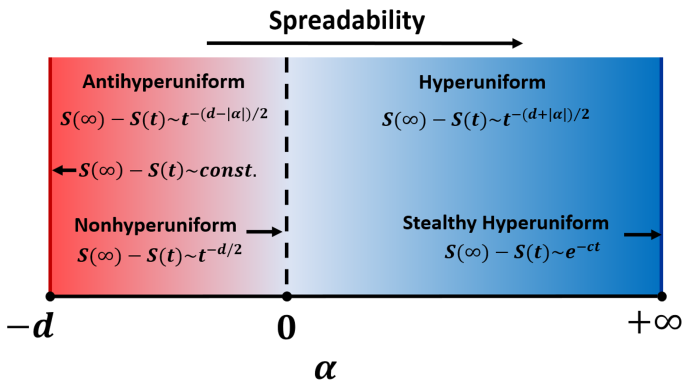
Figure 9: “Phase diagram” that schematically shows the spectrum spreadability regimes in terms of the exponent $\alpha$. As $\alpha$ increases from the extreme antihyperuniform limit of $\alpha\to-d$, the spreadability decay rate gets faster, i.e., the excess spreadability follows the inverse power law $1/t^{(d+\alpha)/2}$, except when $\alpha\to+\infty$, which corresponds to stealthy hyperuniform media with a decay rate that is exponentially fast.

Diffusion-weighted magnetic resonance imaging (dMRI) has become a powerful tool for imaging water-saturated biological media Wedeen et al. (2005). For the purpose of modeling water diffusion in muscles and brain tissue, Novikov et al. Novikov et al. (2014) considered various one-dimensional models in which diffusion is hindered by permeable barriers and estimated the corresponding long-time behaviors of the time-dependent diffusion coefficient ${\cal D}(t)$. Based on this one-dimensional analysis, they were able to extend their findings to any space dimension and found the following long-time scaling behavior of $D(t)$:

$${\cal D}(t)-{\cal D}_{e}\sim\frac{\mbox{C}}{t^{\varphi}},$$ (79)

where $C$ is an undetermined structure-dependent constant and the exponent $\varphi=(d+\alpha)/2$. Remarkably, we see that the long-time behavior of ${\cal D}(t)-{\cal D}_{e}$ is identical to the excess spreadability ${\cal S}(\infty)-{\cal S}(t)$, as specified by the explicit scaling law (36). While the spreadability problem is substantially simpler than the determination of the effective time-dependent diffusion, it is seen that, apart from constants, one can map the former to the latter problem at long times via the transformations ${\cal S}(t)\rightarrow D(t)$ and ${\cal S}(\infty)\rightarrow{\cal D}_{e}={\cal D}(\infty)$.

VII Discussion

Our investigation has demonstrated that the spreadability of diffusion information ${\cal S}(t)$ across time scales has the potential to serve as a powerful dynamic figure of merit to probe and classify all translationally invariant two-phase microstructures across length scales. We established that the small-time behavior of ${\cal S}(t)$ is determined by the derivatives of the autocovariance function $\chi_{{}_{V}}({\bf r})$ at the origin, the leading term of order $t^{1/2}$ being proportional to the specific surface $s$. We proved that the corresponding long-time behavior is determined by the form of the spectral density ${\tilde{\chi}_{{}_{V}}}({\bf k})$ at small wavenumbers, which enables one to ascertain the class of hyperuniform and nonhyperuniform media.

In instances in which the spectral density has the power-law form ${\tilde{\chi}_{{}_{V}}}({\bf k})\sim|{\bf k}|^{\alpha}$ in the limit $|{\bf k}|\to 0$, the long-time excess spreadability for two-phase media in $\mathbb{R}^{d}$ is given by the following inverse power-law decay:

$${\cal S}(\infty)-{\cal S}(t)\sim\frac{1}{t^{(d+\alpha)/2}}.$$ (80)

Observe that this formula can distinguish among the possible strongest forms of hyperuniformity, i.e., class I, according to the value of the exponent for any $\alpha>1$; the larger the value of $\alpha$ for such media, the faster the decay rate the spreadability. The limit $\alpha\to+\infty$ corresponds to media in which the decay rate of ${\cal S}$ is faster than any inverse power law, which we showed is the case for stealthy hyperuniform media. A measured long-time decay rate of ${\cal S}(\infty)-{\cal S}(t)\sim t^{-d/2}$, i.e., the case $\alpha=0$ in (80), would reveal a nonhyperuniform medium in which the spectral density is a bounded positive number at the origin. On the other hand, antihyperuniform media (with $-d<\alpha<0$) have the slowest decay among all translationally invariant media, the slowest being when ${\cal S}(\infty)-{\cal S}(t)$ approaches a constant value (i.e., $\alpha\to-d$), independent of time. The stealthy hyperuniform class is characterized by an excess spreadability with the fastest decay rate (exponentially fast) among all hyperuniform media and hence all translationally invariant microstructures. In short, the spreadability provides a dynamic means to classify the spectrum of possible microstructures that span between hyperuniform and nonhyperuniform media, which is schematically illustrated in Figure 9. Thus, in addition to the usual structure-based methods to ascertain the hyperuniformity/nonhyperuniformity of two-phase media discussed in Sec. II.3, the spreadability at long times provides an alternative dynamic probe of such large-scale structural characteristics.

We obtained exact results for ${\cal S}(t)$ as a function of time for a variety of specific ordered and disordered model microstructures across dimensions, including antihyperuniform media, nonhyperuniform Debye random media, nonstealthy hyperuniform media, disordered stealthy media and periodic media. We also demonstrated that the microstructures with “fast” spreadabilities are also those that can be derived from efficient “coverings” of Euclidean space $\mathbb{R}^{d}$. Finally, we identified a remarkable connection between the spreadability ${\cal S}(t)$ and noninvasive nuclear magnetic resonance (NMR) relaxation measurements in physical and biological porous media Brownstein and Tarr (1979); Mitra et al. (1992, 1993); Sen and Hürlimann (1994); Øren et al. (2002); Wedeen et al. (2005); Novikov et al. (2014).

An interesting avenue for future work is the generalization of the spreadability problem by relaxing Prager’s assumption that the diffusion coefficients of both phases are identical. This more general situation will involve expressions for ${\cal S}(t)$ that now will not only involve the volume fractions and $S_{2}^{(i)}$, but all higher-order correlation functions $S_{3}^{(i)},S_{4}^{(i)},\ldots$ as well as the ratio of the phase diffusion coefficients. The solution of this general problem could be approached using a similar formalism as the “strong-contrast” methodology that has been developed to derive exact expressions for the effective conductivity of two-phase media in terms of this infinite set of correlation functions and phase contrast ratio Sen and Torquato (1989); Torquato (2002).

Appendix A Moments of the Autocovariance Function for the Disordered Hyperuniform Model

Here we provide simplified closed-form expressions obtained from the general formula (56) for the $n$th-order moment of the autocovariance function (50) for the special cases in the first three space dimensions considered in Sec. IV.2. Specifically, for $d=1$ with $qa=1$, and $c=\sqrt{2}$ and $\theta=\pi/4$, we find

$$M_{n}(\chi_{{}_{V}})=-\phi_{1}\phi_{2}\frac{n!}{2^{n/2}}\sin(n\pi/4)\quad(d=1).$$ (81)

Similarly, with $\theta=0$, $c=1$, we have for $d=2$ with $qa=1$,

$$M_{n}(\chi_{{}_{V}})=\phi_{1}\phi_{2}\frac{n!}{2^{(n+1)/2}}\cos[(n+1)\pi/4]\quad(d=2)$$ (82)

and for $d=3$ with $(qa)^{2}=1/3$,

$$M_{n}(\chi_{{}_{V}})=\phi_{1}\phi_{2}\frac{n!3^{(n+1)/2}}{2^{n+1}}\cos[(n+1)\pi/6)]\quad(d=3).$$ (83)

Appendix B Some $d$-Dimensional Crystal Structures

Here, we define some well-known crystal structures, including (Bravais) lattices as well as lattices with a basis, what we generally call periodic point configurations Torquato (2010). Some commonly known $d$-dimensional lattices include the hypercubic $\mathbb{Z}^{d}$, checkerboard $D_{d}$, and root $A_{d}$ lattices, defined, respectively, by

$${\mathbb{Z}^{d}=\{(x_{1},\ldots,x_{d}):x_{i}\in}{{\mathbb{Z}}}{\}\quad\mbox{for}\;d\geq 1}$$ (84)

$${D_{d}=\{(x_{1},\ldots,x_{d})\in\mathbb{Z}^{d}:x_{1}+\cdots+x_{d}~{}~{}\mbox{even}\}\quad\mbox{for}\;d\geq 3}$$ (85)

$$A_{d} = \{(x_{0},x_{1},\ldots,x_{d})\in\mathbb{Z}^{d+1}:x_{0}+x_{1}+\cdots+x_{d}=0\}$$ (86)

$$\quad\mbox{for}\;d\geq 1,$$

where $\mathbb{Z}$ is the set of integers ($\ldots-3,-2,-1,0,1,2,3\ldots$); $x_{1},\ldots,x_{d}$ denote the components of a lattice vector of either $\mathbb{Z}^{d}$ or $D_{d}$; and $x_{0},x_{1},\ldots,x_{d}$ denote a lattice vector of $A_{d}$. The $d$-dimensional lattices $\mathbb{Z}^{d}_{*}$, $D_{d}^{*}$ and $A_{d}^{*}$ are the corresponding dual (or reciprocal) lattices. Following Conway and Sloane Conway and Sloane (1998) , we say that two lattices are equivalent or similar if one becomes identical to the other possibly by a rotation, reflection, and change of scale, for which we use the symbol $\equiv$. The $A_{d}$ and $D_{d}$ lattices can be regarded as $d$-dimensional generalizations of the face-centered-cubic (FCC) lattice defined by $A_{3}\equiv D_{3}$; however, for $d\geq 4$, they are no longer equivalent. In two dimensions, $A_{2}\equiv A_{2}^{*}$ defines the triangular lattice with a dual lattice that is equivalent. In three dimensions, $A_{3}^{*}\equiv D_{3}^{*}$ defines the body-centered-cubic (BCC) lattice. In four dimensions, the checkerboard lattice and its dual are equivalent, i.e., $D_{4}\equiv D_{4}^{*}$. The hypercubic lattice $\mathbb{Z}^{d}\equiv\mathbb{Z}^{d}_{*}$ and its dual lattice are equivalent for all $d$.

We denote by $\mbox{Dia}_{d}$ and $\mbox{Kag}_{d}$ the crystals that are $d$-dimensional generalizations of the diamond and kagomé crystals, respectively, for $d\geq 2$ Zachary and Torquato (2011). While the crystal $\mbox{Dia}_{d}$ has a two-particle basis (independent of $d$), the crystal $\mbox{Kag}_{d}$ as a ($d+1$)-particle basis.

Appendix C Spreadability for 1D Integer Lattice Packings

Here we derive an exact expression for the spreadability for all times for the special case of one-dimensional packings of identical rods of radius $a$ (length $2a$) centered on the sites of the integer lattice $\mathbb{Z}$ with lattice spacing $L$, so that $Q_{n}=2\pi n/L$ and $\phi_{2}=2a/L$. Application of the general formula (73) in the case of the 1D integer lattice packing, where $Z(Q_{n})=2$ for all $n$, yields

$${\cal S}(\infty)-{\cal S}(t) = \phi_{2}\sum_{n=1}^{\infty}\frac{{\tilde{\alpha}}(2\pi na/L)}{a}\exp[-(2\pi n)^{2}Dt/L^{2}]$$

$$= \frac{2}{\,\phi_{2}\,\pi^{2}}\sum_{n=1}^{\infty}\frac{\sin^{2}(\pi n\phi_{2})}{n^{2}}\exp[-(2\pi n)^{2}Dt/L^{2}].$$

Note that because ${\cal S}(t=0)=0$, we have the identity

$$\frac{1}{\pi^{2}}\sum_{n=1}^{\infty}\frac{\sin^{2}(\pi n\phi_{2})}{n^{2}}=\frac{\phi_{1}\phi_{2}}{2}.$$ (88)

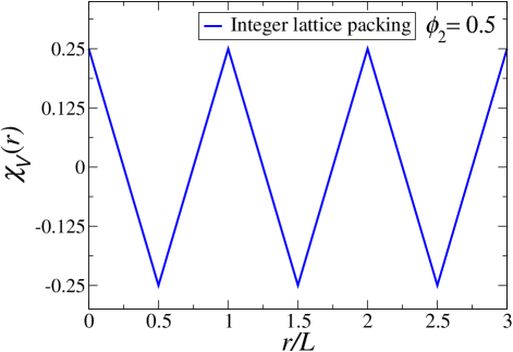
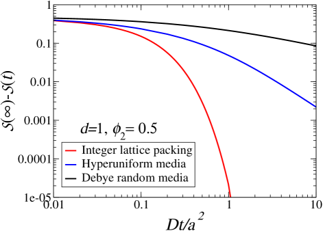
Figure 10: Top panel: The autocovariance function $\chi_{{}_{V}}(r)$ versus $r/L$ for the integer lattice packing for the instance $\phi_{2}=0.5$, where $L$ is the lattice spacing. Bottom panel: Excess spreadability ${\cal S}(\infty)-{\cal S}(t)$ versus dimensionless time $Dt/a^{2}$ for short times for three different models: integer lattice packing, nonstealthy disordered hyperuniform media and (nonhyperuniform) Debye random media, each with $\phi_{2}=0.5$.

The autocovariance function $\chi_{{}_{V}}(r)$ for the integer lattice packing for the instance $\phi_{2}$ and the corresponding excess spreadability for small times is shown in Fig. 1. The latter plot compares ${\cal S}(\infty)-{\cal S}(t)$ to those of the 1D models of (nonhyperuniform) Debye random media and nonstealthy disordered hyperuniform media, as discussed in Sec. IV.1 and Sec. IV.2, respectively. It is noteworthy that when $Dt/a^{2}=1$, the excess spreadability for periodic media is already about four orders of magnitude smaller than that of nonstealthy disordered hyperuniform media.