DeepStationing: Thoracic Lymph Node Station Parsing in CT Scans using Anatomical Context Encoding and Key Organ Auto-Search

Abstract

LNS delineation from CT scans is an indispensable step in radiation oncology workflow. High inter-user variabilities across oncologists and prohibitive laboring costs motivated the automated approach. Previous works exploit anatomical priors to infer LNS based on predefined ad-hoc margins. However, without the voxel-level supervision, the performance is severely limited. LNS is highly context-dependent—LNS boundaries are constrained by anatomical organs—we formulate it as a deep spatial and contextual parsing problem via encoded anatomical organs. This permits the deep network to better learn from both CT appearance and organ context. We develop a stratified referencing organ segmentation protocol that divides the organs into anchor and non-anchor categories and uses the former’s predictions to guide the later segmentation. We further develop an auto-search module to identify the key organs that opt for the optimal LNS parsing performance. Extensive four-fold cross-validation experiments on a dataset of $98$ esophageal cancer patients (with the most comprehensive set of 12 LNS + 22 organs in thoracic region to date) are conducted. Our LNS parsing model produces significant performance improvements, with an average Dice score of $81.1\%\pm 6.1\%$, which is $5.0\%$ and $19.2\%$ higher over the pure CT-based deep model and the previous representative approach, respectively.

1 Introduction

Cancers in thoracic region are the most common cancers worldwide [17] and significant proportions of patients are diagnosed at late stages involved with lymph node (LN) metastasis. The treatment protocol is a sophisticated combination of surgical resection and chemotherapy and/or radiotherapy [5]. Assessment of involved LNs [21, 1] and accurate labeling their corresponding stations are essential for the treatment selection and planning. For example, in radiation therapy, the delineation accuracy of gross tumor volume (GTV) and clinical target volume (CTV) are the two most critical factors impacting the patient outcome. For CTV delineation, areas containing metastasis LN should be included to sufficiently cover the sub-clinical disease regions [2]. One strategy to outline the sub-clinical disease region is to include the LNS that containing the metastasized LN [14, 19]. Thoracic LNS is determined according to the text definitions of IASLC [15]. The delineation of LNS in the current clinical workflow is predominantly a manual process using CT images. Visual assessment and manual delineation is a challenging and time-consuming task even for experienced physicians, since converting text definitions of IASLC to precise 3D voxel-wise annotations can be error prone leading to large intra- and inter-user variability [2].

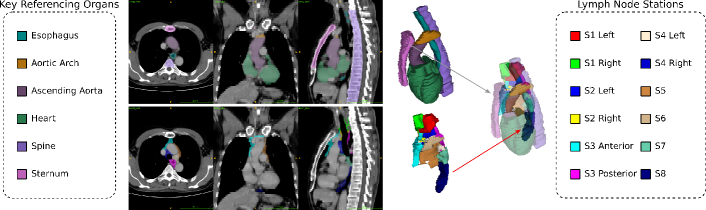
Figure 1: An illustration of LNS and key referencing organs. The top row illustrates the auto-searched top-6 key referencing organs; the bottom row depicts the 12 LNS.

Deep CNN have made remarkable progress in segmenting organs and tumors in medical imaging [18, 20, 7, 8, 4, 9]. Only a handful of non-deep learning studies have tackled the automated LNS segmentation [3, 13, 16, 11]. A LNS atlas was established using deformable registration [3]. Predefined margins from manually selected organs, such as the aorta, trachea, and vessels, were applied to infer LNS [11], which was not able to accurately adapt to individual subject. Other methods [13, 16] built fuzzy models to directly parse the LNS or learn the relative positions between LNS and some referencing organs. Average location errors ranging from $6.9$mm to $34.2$mm were reported using 22 test cases in [13], while an average Dice score (DSC) of $66.0\%$ for $10$ LNSs in 5 patients was observed in [16].

In this work, we propose the DeepStationing – an anatomical context encoded deep LNS parsing framework with key organ auto-search. We first segment a comprehensive set of 22 chest organs related to the description of LNS according to IASLC guideline. As inspired by [4], the 22 organs are stratified into the anchor or non-anchor categories. The predictions of the former category are exploited to guide and boost the segmentation performance of the later category. Next, CT image and referencing organ predictions are combined as different input channels to the LNS parsing module. The 22 referencing organs are identified by human experts. However, relevant but different from the human process, CNN may require a particular set of referencing organs (key organs) that can opt for optimal performance. Therefore, we automatically search for the key organs by applying a channel-weighting to the input organ prediction channels based on differentiable neural search [10]. The auto-searched final top-6 key organs, i.e., esophagus, aortic arch, ascending aorta, heart, spine and sternum (shown in Fig. 1), facilitate our DeepStationing method to achieve high LNS parsing accuracy. We adopt 3D nnU-Net [6] as our segmentation and parsing backbone. Extensive 4-fold cross-validation is conducted using a dataset of $98$ CT images with $12$ LNS + $22$ Organ labels each, as the first of its kind to date. Experimental results demonstrate that deep model encoded with the spatial context of auto-searched key organs significantly improves the LNS paring performance, resulting in an average DS of $81.1\%\pm 6.1\%$, which is $5.0\%$ and $19.2\%$ higher over the pure CT-based deep model and the most recent relevant work [11] (from our re-implementations), respectively.

2 Method

Fig. 2 depicts the overview of our DeepStationing framework, consisting of two major modularized components: (1) stratified chest organ segmentation; (2) context encoded LNS parsing with key organ auto-search.

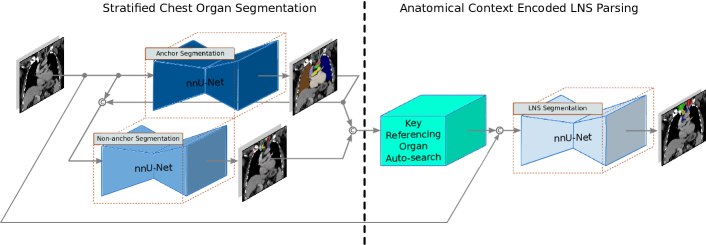
Figure 2: Overall workflow of our DeepStationing, which consists of stratified chest organ segmentation and anatomical context encoded LNS parsing with key organ auto-search.

2.1 Stratified Chest Organ Segmentation

To provide the spatial context for LNS parsing, we first segment a comprehensive set of 22 chest organs related to the description of LNS. Simultaneously segmenting a large number of organs increase optimization difficulty leading to sub-optimal performance. Motivated by  [4], we stratify 22 chest organs into the anchor and non-anchor categories. Anchor organs have high contrast, hence, it is relatively easy and robust to segment them directly using the deep appearance features. Anchor organs are first segmented, and their results serve as ideal candidates to support the segmentation of other difficult non-anchors. We use two CNN branches to stratify the anchor and non-anchor organ segmentation. With predicted anchor organs as additional input, the non-anchor organs are segmented. Assuming $N$ data instances, we denote the training data as $\mathbb{S}=\left\{X_{n},Y_{n}^{\mathrm{A}},Y_{n}^{\mathrm{\neg A}},Y_{n}^{\mathrm{L}},\right\}_{n=1}^{N}$, where $X_{n}$, $Y_{n}^{\mathrm{A}}$, $Y_{n}^{\mathrm{\neg A}}$ and $Y_{n}^{\mathrm{L}}$ denote the input CT and ground-truth masks for the anchor, non-anchor organs and LNS, respectively. Assuming there are $C_{\mathrm{A}}$ and $C_{\mathrm{\neg A}}$ classes for anchor and non-anchor organs and dropping $n$ for clarity, our organ segmentation module generate the anchor and non-anchor organ predictions at every voxel location, $j$, and every output class, $c$:

$$\hat{Y}^{\mathrm{A}}_{c}(j)=p^{\mathrm{A}}\left(Y^{\mathrm{A}}(j)=c\,|\,X;\mathbf{W}^{\mathrm{A}}\right)\mathrm{,} \quad\hat{\mathbf{Y}}^{\mathrm{A}}=\left[\hat{Y}^{\mathrm{A}}_{1}\ldots\hat{Y}^{\mathrm{A}}_{C_{\mathrm{A}}}\right]\mathrm{,}$$ (1)

$$\hat{Y}^{\mathrm{\neg A}}_{c}(j)=p^{\mathrm{\neg A}}\left(Y^{\mathrm{\neg A}}(j)=c\,|\,X,\hat{\mathbf{Y}}^{\mathrm{A}};\mathbf{W}^{\mathrm{\neg A}}\right)\mathrm{,} \quad\hat{\mathbf{Y}}^{\mathrm{\neg A}}=\left[\hat{Y}^{\mathrm{\neg A}}_{1}\ldots\hat{Y}^{\mathrm{\neg A}}_{C_{\mathrm{\neg A}}}\right]\mathrm{,}$$ (2)

where $p^{(\ast)}(.)$ denotes the CNN functions and and $\hat{Y}^{(\ast)}_{c}$ for the output segmentation maps. Here, we combine both anchor and non-anchor organ predictions into an overall prediction map $\hat{\mathbf{Y}}^{\mathfrak{A}}=\hat{\mathbf{Y}}^{\mathrm{A}}\cup\hat{\mathbf{Y}}^{\mathrm{\neg A}}$. Predictions are vector valued 3D masks as they provide a pseudo-probability for every class. $\mathbf{W}^{(\ast)}$ represents the corresponding CNN parameters.

2.2 Anatomical Context Encoded LNS Parsing

Segmenting LNS by only CT appearance can be error prone, since LNS highly relies on the spatial context of adjacent anatomical structures. Emulating the clinical practice of IASLC guidelines, we incorporate the referencing organs into the training process of LNS parsing. Given $C_{\mathrm{L}}$ classes of the LNS, as illustrated in Fig. 2, we combine the above organ predictions with CT images to create a multi-channel input: $\left[X,\,\,\hat{\mathbf{Y}}^{\mathfrak{A}}\right]$:

$$\hat{Y}^{\mathrm{L}}_{c}(j)=p^{\mathrm{L}}\left(Y^{\mathrm{L}}(j)=c\,|\,X,\hat{\mathbf{Y}}^{\mathfrak{A}};\mathbf{W}^{\mathrm{L}}\right)\mathrm{,}\quad\hat{\mathbf{Y}}^{\mathrm{L}}=\left[\hat{Y}^{\mathrm{L}}_{1}\ldots\hat{Y}^{\mathrm{L}}_{C_{\mathrm{L}}}\right]\mathrm{.}$$ (3)

Thereupon, the LNS parsing module leverages both the CT appearance and the predicted anatomical structures, implicitly encoding the spatial distributions of referencing organs during training. Similar to Eq. (1), we have the LNS prediction in its vector-valued form as $\hat{\mathbf{Y}}^{\mathrm{L}}$.

2.2.1 Key Organ Auto-search

The 22 referencing organs are previously selected according to the IASLC guideline. Nevertheless for deep learning based LNS model training, those manually selected organs might not lead to the optimal performance. Considering the potential variations in organ location and size distributions, and differences in automated organ segmentation accuracy, we hypothesize that the deep LNS parsing model would benefit from an automated reference organ selection process that are tailored to this purpose. Hence, we use the differentiable neural search [4] to search the key organs by applying a channel-weighting strategy to input organ masks. We make the search space continuous by relaxing the selection of the referencing organs to a Softmax function over the channel weights of the one-hot organ predictions $\hat{\mathbf{Y}}^{\mathfrak{A}}$. For $C_{\mathrm{L}}$ classes, we define a set of $C_{\mathrm{L}}$ learn-able logits for each channel, denoted as $\alpha_{c},\forall c\in\left[1\cdots C_{\mathrm{L}}\right]$. The channel weight $\phi_{c}$ for a referencing organ is defined as:

$$\phi_{c}=\dfrac{\text{exp}\left(\alpha_{c}\right)}{\sum_{m=1}^{C_{\mathrm{L}}}\text{exp}\left(\alpha_{m}\right)} \mathrm{,}\quad\Phi=\left[\phi_{1}\cdots\phi_{C_{\mathrm{L}}}\right]\mathrm{,}$$ (4)

$$F(\hat{Y}^{\mathfrak{A}}_{c},\phi_{c})=\phi_{c}\cdot\hat{Y}^{\mathfrak{A}}_{c} \mathrm{,}\quad F(\hat{\mathbf{Y}}^{\mathfrak{A}},\Phi)=\left[F(\hat{Y}^{\mathfrak{A}}_{1},\phi_{1})\cdots F(\hat{Y}^{\mathfrak{A}}_{C_{\mathrm{L}}},\phi_{C_{\mathrm{L}}})\right]$$ (5)

where $\Phi$ denotes the set of channel weights and $F(\phi_{c},\hat{Y}^{\mathfrak{A}}_{c})$ denotes the channel-wise multiplication between the scalar $\phi_{c}$ and the organ prediction $\hat{Y}^{\mathfrak{A}}_{c}$. The input of LNS parsing model becomes $\left[X,\,\,F(\hat{\mathbf{Y}}^{\mathfrak{A}},\Phi)\right]$. As the results of the key organ auto-search, we select the organs with the top-$n$ weights to be the searched $n$ key organs. In this paper, we heuristically select the $n=6$ based on the experimental results. Last, we train the LNS parsing model using the combination of original CT images and the auto-selected top-$6$ key organs’ segmentation predictions.

3 Experimental Results

Dataset. We collected $98$ contrast-enhanced venous-phase CT images of patients with esophageal cancers underwent surgery and/or radiotherapy treatments. A board-certified radiation oncologist with 15 years of experience annotated each patient with 3D masks of $12$ LNS, involved LN (if any), and $22$ referencing organs related to LNS according to IASLC guideline. The 12 annotated LN stations are: S1 (left + right), S2 (left + right), S3 (anterior + posterior), S4 (left + right), S5, S6, S7, S8. The average CT image size is $512\times 512\times 80$ voxels with an average resolution of $0.7\times 0.7\times 5.0$mm. Extensive four-fold cross-validation (CV), separated at the patient level, was conducted. We report the segmentation performance using DS in percentage, HD and ASD in mm.

Table 1: Mean DSCs, HDs, and ASDs, and their standard deviations of LNS parsing performance using: (1) only CT appearance; (2) CT$+$all 22 referencing organ ground-truth masks; (3) CT$+$all 22 referencing organ predicted masks; (4) CT$+$auto-searched 6 referencing organ predicted masks. The best performance scores are shown in bold.

LNS	CT Only	+22 Organ GT	+22 Organ Pred	+6 Searched Organ Pred
DSC
S1 Left	78.1 $\pm$ 6.8	84.3 $\pm$ 4.5	82.3 $\pm$ 4.6	85.1 $\pm$ 4.0
S1 Right	76.8 $\pm$ 5.0	84.3 $\pm$ 3.4	82.2 $\pm$ 3.4	85.0 $\pm$ 4.1
S2 Left	66.9 $\pm$ 11.4	75.8 $\pm$ 9.0	73.7 $\pm$ 8.9	76.1 $\pm$ 8.2
S2 Right	70.7 $\pm$ 8.5	74.8 $\pm$ 7.6	72.8 $\pm$ 7.6	77.5 $\pm$ 6.4
S3 Anterior	77.4 $\pm$ 4.9	79.8 $\pm$ 5.6	79.7 $\pm$ 5.6	81.5 $\pm$ 4.9
S3 Posterior	84.6 $\pm$ 3.1	87.9 $\pm$ 2.8	87.8 $\pm$ 2.9	88.6 $\pm$ 2.7
S4 Left	74.1 $\pm$ 8.2	77.0 $\pm$ 8.9	76.9 $\pm$ 8.9	77.9 $\pm$ 9.4
S4 Right	73.8 $\pm$ 8.9	74.9 $\pm$ 9.3	74.9 $\pm$ 9.4	76.7 $\pm$ 8.3
S5	72.6 $\pm$ 6.7	73.2 $\pm$ 7.4	73.2 $\pm$ 7.4	77.9 $\pm$ 8.0
S6	72.4 $\pm$ 5.7	74.9 $\pm$ 4.4	74.8 $\pm$ 4.5	75.7 $\pm$ 4.3
S7	85.0 $\pm$ 5.1	86.6 $\pm$ 5.8	86.6 $\pm$ 5.8	88.0 $\pm$ 6.1
S8	80.9 $\pm$ 6.1	84.0 $\pm$ 5.9	82.0 $\pm$ 5.9	84.3 $\pm$ 6.3
Average	76.1 $\pm$ 6.7	79.8 $\pm$ 6.2	78.9 $\pm$ 6.3	81.1 $\pm$ 6.1
HD
S1 Left	11.9 $\pm$ 3.2	12.3 $\pm$ 6.0	27.6 $\pm$ 38.8	10.3 $\pm$ 4.1
S1 Right	18.0 $\pm$ 29.3	10.6 $\pm$ 2.6	61.1 $\pm$ 97.6	9.7 $\pm$ 1.8
S2 Left	13.3 $\pm$ 9.2	9.7 $\pm$ 3.1	35.6 $\pm$ 76.9	9.2 $\pm$ 3.1
S2 Right	36.3 $\pm$ 61.7	10.8 $\pm$ 3.0	10.8 $\pm$ 3.0	9.5 $\pm$ 3.2
S3 Anterior	41.7 $\pm$ 62.4	13.5 $\pm$ 4.9	50.4 $\pm$ 79.1	12.2 $\pm$ 4.3
S3 Posterior	9.1 $\pm$ 3.3	8.0 $\pm$ 2.0	18.0 $\pm$ 30.9	7.6 $\pm$ 1.9
S4 Left	11.5 $\pm$ 4.9	14.7 $\pm$ 22.2	14.5 $\pm$ 22.2	9.8 $\pm$ 3.8
S4 Right	32.8 $\pm$ 69.7	9.8 $\pm$ 3.5	16.2 $\pm$ 21.5	9.8 $\pm$ 3.6
S5	36.4 $\pm$ 56.4	20.5 $\pm$ 35.2	38.1 $\pm$ 60.3	10.9 $\pm$ 4.0
S6	19.2 $\pm$ 30.6	8.6 $\pm$ 2.5	52.5 $\pm$ 85.3	8.5 $\pm$ 2.7
S7	26.3 $\pm$ 42.6	9.6 $\pm$ 3.7	9.6 $\pm$ 3.7	9.5 $\pm$ 3.5
S8	14.5 $\pm$ 6.0	13.6 $\pm$ 5.7	13.1 $\pm$ 5.8	12.2 $\pm$ 6.2
Average	22.6 $\pm$ 31.6	11.8 $\pm$ 7.9	28.9 $\pm$ 43.8	9.9 $\pm$ 3.5
ASD
S1 Left	1.6 $\pm$ 0.8	1.3 $\pm$ 0.6	1.4 $\pm$ 1.0	0.9 $\pm$ 0.5
S1 Right	1.8 $\pm$ 0.8	1.2 $\pm$ 0.5	1.6 $\pm$ 1.1	0.9 $\pm$ 0.5
S2 Left	1.4 $\pm$ 0.8	1.0 $\pm$ 0.6	1.3 $\pm$ 0.8	0.8 $\pm$ 0.6
S2 Right	1.5 $\pm$ 0.8	1.3 $\pm$ 0.7	1.3 $\pm$ 0.7	1.0 $\pm$ 0.7
S3 Anterior	1.0 $\pm$ 0.8	0.7 $\pm$ 0.4	0.9 $\pm$ 0.9	0.6 $\pm$ 0.4
S3 Posterior	0.9 $\pm$ 0.5	0.6 $\pm$ 0.3	0.8 $\pm$ 1.1	0.6 $\pm$ 0.4
S4 Left	1.0 $\pm$ 0.6	1.4 $\pm$ 2.7	1.2 $\pm$ 1.6	0.8 $\pm$ 0.6
S4 Right	1.5 $\pm$ 1.0	1.4 $\pm$ 1.0	1.5 $\pm$ 1.0	1.3 $\pm$ 1.0
S5	1.3 $\pm$ 0.6	1.9 $\pm$ 3.4	1.6 $\pm$ 1.8	1.0 $\pm$ 0.5
S6	0.8 $\pm$ 0.4	0.7 $\pm$ 0.3	1.0 $\pm$ 1.1	0.6 $\pm$ 0.3
S7	0.9 $\pm$ 0.7	0.8 $\pm$ 0.6	0.8 $\pm$ 0.6	0.7 $\pm$ 0.6
S8	1.7 $\pm$ 1.2	1.6 $\pm$ 1.1	1.6 $\pm$ 1.1	1.3 $\pm$ 1.3
Average	1.3 $\pm$ 0.7	1.1 $\pm$ 1.0	1.3 $\pm$ 1.1	0.9 $\pm$ 0.6

Implementation details. We adopt the nnU-Net [6] with DSC+CE losses as our backbone for all experiments due to its high accuracy on many medical image segmentation tasks. The nnU-Net has been proposed to automatically adapt different preprocessing strategies (i.e., the training image patch size, resolution, and learning rate) to a given 3D medical imaging dataset. We use the default nnU-Net settings for our model training. The total training epochs is 1000. For the organ auto-search parameter $\alpha_{c}$, we first fix the $\alpha_{c}$ for $200$ epochs and alternatively update the $\alpha_{c}$ and the network weights for another $800$ epochs. The rest settings are the same as the default nnU-Net setup. We implemented our DeepStationing method in PyTorch, and an NVIDIA Quadro RTX 8000 was used for training. The average training/inference time is 2.5 GPU days or 3 mins.

Quantitative Results.

We first evaluate the performance of our stratified referencing organ segmentation. The average DSC, HD and ASD for anchor and nonanchor organs are $90.0\pm 4.3\%$, $16.0\pm 18.0mm$, $1.2\pm 1.1mm$, and $82.1\pm 6.0\%$, $19.4\pm 15.0mm$, $1.2\pm 1.4mm$, respectively. We also train a model by segmenting all organs using only one nnUNet. The average DSCs of the anchor, non-anchor, and all organs are $86.4\pm 5.1\%$, $72.7\pm 8.7\%$, and $80.8\pm 7.06\%$, which are $3.6\%$, $9.4\%$, and $5.7\%$ less than the stratified version, respectively. The stratified organ segmentation demonstrates high accuracy, which provides robust organ predictions for the subsequent LNS parsing model.

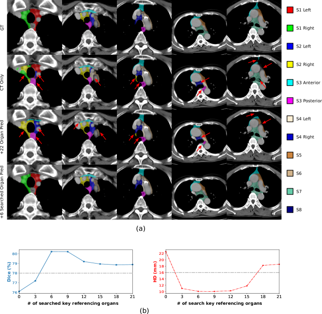
Figure 3: (a) Examples of LNS parsing results using different setups. For better comparison, red arrows are used to depict visual improvements. (b) The bottom charts demonstrate the performance using different numbers of searched referencing organs.

Table 1 outlines the quantitative comparisons on different deep LNS parsing setups. Columns 1 to 3 show the results using: 1) only CT images, 2) CT $+$ all $22$ ground-truth organ masks, and 3) CT $+$ all $22$ predicted organ masks. Using only CT images, LNS parsing exhibits lowest performance with an average DS of $76.1\%$ and HD of $22.6$mm. E.g., distant false predictions is observed in the first image $2^{nd}$ row of Fig. 3 and false-positive S3 posterior is predicted (in pink) between the S1 and S2. When adding $22$ ground-truth organ masks as spatial context, both DS and HD show remarked improvements: from $76.1\%$ to $79.8\%$ in DS and $22.6$mm to $11.8$mm in HD. This verifies the importance and effectiveness of referencing organs in inferring LNS boundaries. However, when predicted masks of the 22 organs are used (the real testing condition), it has a significant increase in HD from $11.8$mm to $28.9$mm as compared to that using ground truth organ masks. This shows the necessity to select the key organs suited for the deep parsing model. Finally, using the top-6 auto-searched referencing organs, our DeepStationing model achieves the best performance reaching 81.1 $\pm$ 6.1% DSC, 9.9 $\pm$ 3.5mm HD and 0.9 $\pm$ 0.6mm ASD. Qualitative examples are shown in Fig. 3 illustrating these performance improvements.

We auto-search for the organs that are tailored to optimize the LNS parsing performance. Using an interval of 3, we train 7 additional LNS parsing models, by including the top-3 up to top-21 organs. The auto-searched ranking of the 22 organs is listed as follows: esophagus, aortic arch, ascending aorta, heart, spine, sternum, V.BCV (R+L), V.pulmonary, descending aorta, V.IJV (R+L), A.CCA (R+L), V.SVC, A.pulmonary, V.azygos, bronchus (R+L), lung (R+L), trachea, where ‘A’ and ‘V’ denote the Artery and Vein. The quantitative LNS parsing results in selecting the top-n organs are illustrated in the bottom charts of Fig. 3. With more organs included gradually, the DS first improves, then slightly drops after having more than top-6 organs. The performance later witnesses a sharp drop after including more than top-9 organs, then becoming steady when we include more than top-15 organs. This demonstrates that deep LNS paring model does not need a complete set of referencing organs to capture the LNS boundaries. We choose the top-6 as our final key organs based on experimental results. We notice that the trachea, lungs, and bronchus are surprisingly ranked in the bottom-5 of the auto-search, although previous works [12, 11] manually selected them for the LNS parsing. The assumed reasons are that those organs are usually filled with air and have clear boundaries while LNS does not include air or air-filled organs. With the help of the other found key organs, it is relatively straightforward for the LNS parsing CNN to distinguish them and reject the false-positives located in those air-filled organs. We further include 6 ablation studies and segment LNS using: (1) randomly selected 6 organs; (2) top-6 organs with best organ segmentation accuracy; (3) anchor organs; (4) recommended 6 organs from the senior oncologists; (5) searched 6 organs predictions from less accurate non-stratified organ segmentor; (6) searched 6 organs GT. The randomly selected 6 organs are: V.BCV (L), V.pulmonary, V.IJV (R), heart, spine, trachea; The 6 organs with the best segmentation accuracy are: lungs (R+L), descending aorta, heart, trachea, spine; Oncologists recommended 6 organs are: trachea, aortic arch, spine, lungs (R+L), descending aorta; The DSCs for setups (1-6) are 77.2%, 78.2%, 78.6%, 79.0%, 80.2%, 81.7%; the HDs are 19.3mm, 11.8mm, 12.4mm, 11.0mm, 10.1mm, 8.6mm, respectively. In comparison to the LNS predictions using only CT images, the ablation studies demonstrate that using the referencing organ for LNS segmentation is the key contributor for the performance gain, and the selection and the quality of supporting organs are the main factors for the performance boost, e.g., our main results of the setups (5) and (6) show that better searched-organ delineation can help get superior LNS segmentation performance.

Comparison to previous work. We compare the DeepStationing to the previous most relevant approach [11] that exploits heuristically pre-defined spatial margins for LNS inference. The DeepStationing outperforms  [11] by $19.2\%$ in DS, $30.2$mm in HD, and $5.2$mm in ASD. For the ease of comparison, similar to [11], we also merge our LNS into four LN zones, i.e., supraclavicular (S1), superior (S2, S3, and S4), aortic (S5 and S6) and inferior (S7 and S8) zones, and calculate the accuracy of LN instances that are correctly located in the predicted zones. DeepStationing achieves an average accuracy of $96.5\%$, or $13.3\%$ absolutely superior than [11] in LN instance counting accuracy. We tested additionally 2 backbone networks: 3D PHNN (3D UNet with a light-weighted decoding path) and 2D UNet. The DSCs of 3D PHNN and 2D UNet are 79.5% and 78.8%, respectively. The assumed reason for the performance drop might be the loss of the boundary precision/3D information.

4 Conclusion

In this paper, we propose DeepStationing as a novel framework that performs key organ auto-search based LNS parsing on contrasted CT images. Emulating the clinical practices, we segment the referencing organs in thoracic region and use the segmentation results to guide LNS parsing. Different from employing the key organs directly suggested by oncologists, we search for the key organs automatically as a neural architecture search problem that can opt for optimal performance. Evaluated using a most comprehensive LNS dataset, DeepStationing method outperforms previous most relevant approach by a significant quantitative margin of $19.2\%$ in DS, and is coherent to clinical explanation. This work is an important step towards reliable and automated LNS segmentation.

References

- [1] Chao, C.H., Zhu, Z., Guo, D., Yan, K., Ho, T.Y., Cai, J., Harrison, A.P., Ye, X., Xiao, J., Yuille, A., et al.: Lymph node gross tumor volume detection in oncology imaging via relationship learning using graph neural network. In: International Conference on Medical Image Computing and Computer-Assisted Intervention. pp. 772–782. Springer, Cham (2020)
- [2] Chapet, O., Kong, F.M., Quint, L.E., Chang, A.C., Ten Haken, R.K., Eisbruch, A., Hayman, J.A.: Ct-based definition of thoracic lymph node stations: an atlas from the university of michigan. International Journal of Radiation Oncology* Biology* Physics 63(1), 170–178 (2005)
- [3] Feuerstein, M., Glocker, B., Kitasaka, T., Nakamura, Y., Iwano, S., Mori, K.: Mediastinal atlas creation from 3-d chest computed tomography images: application to automated detection and station mapping of lymph nodes. Medical image analysis 16(1), 63–74 (2012)
- [4] Guo, D., Jin, D., Zhu, Z., Ho, T.Y., Harrison, A.P., Chao, C.H., Xiao, J., Lu, L.: Organ at risk segmentation for head and neck cancer using stratified learning and neural architecture search. In: Proceedings of the IEEE/CVF Conference on Computer Vision and Pattern Recognition. pp. 4223–4232 (2020)
- [5] Hirsch, F.R., Scagliotti, G.V., Mulshine, J.L., Kwon, R., Curran Jr, W.J., Wu, Y.L., Paz-Ares, L.: Lung cancer: current therapies and new targeted treatments. The Lancet 389(10066), 299–311 (2017)
- [6] Isensee, F., Jaeger, P.F., Kohl, S.A., Petersen, J., Maier-Hein, K.H.: nnu-net: a self-configuring method for deep learning-based biomedical image segmentation. Nature Methods pp. 1–9 (2020)
- [7] Jin, D., Guo, D., Ho, T.Y., Harrison, A.P., Xiao, J., Tseng, C.k., Lu, L.: Accurate esophageal gross tumor volume segmentation in pet/ct using two-stream chained 3d deep network fusion. In: International Conference on Medical Image Computing and Computer-Assisted Intervention. pp. 182–191. Springer, Cham (2019)
- [8] Jin, D., Guo, D., Ho, T.Y., Harrison, A.P., Xiao, J., Tseng, C.k., Lu, L.: Deep esophageal clinical target volume delineation using encoded 3d spatial context of tumors, lymph nodes, and organs at risk. In: International Conference on Medical Image Computing and Computer-Assisted Intervention. pp. 603–612. Springer, Cham (2019)
- [9] Jin, D., Guo, D., Ho, T.Y., Harrison, A.P., Xiao, J., Tseng, C.k., Lu, L.: Deeptarget: Gross tumor and clinical target volume segmentation in esophageal cancer radiotherapy. Medical Image Analysis 68, 101909 (2020)
- [10] Liu, H., Simonyan, K., Yang, Y.: Darts: Differentiable architecture search. arXiv preprint arXiv:1806.09055 (2018)
- [11] Liu, J., Hoffman, J., Zhao, J., Yao, J., Lu, L., Kim, L., Turkbey, E.B., Summers, R.M.: Mediastinal lymph node detection and station mapping on chest ct using spatial priors and random forest. Medical physics 43(7), 4362–4374 (2016)
- [12] Lu, K., Taeprasartsit, P., Bascom, R., Mahraj, R.P., Higgins, W.E.: Automatic definition of the central-chest lymph-node stations. International journal of computer assisted radiology and surgery 6(4), 539–555 (2011)
- [13] Matsumoto, M.M., Beig, N.G., Udupa, J.K., Archer, S., Torigian, D.A.: Automatic localization of iaslc-defined mediastinal lymph node stations on ct images using fuzzy models. In: Medical Imaging 2014: Computer-Aided Diagnosis. vol. 9035, p. 90350J. International Society for Optics and Photonics (2014)
- [14] Pignon, J.P., Arriagada, R., Ihde, D.C., Johnson, D.H., Perry, M.C., Souhami, R.L., Brodin, O., Joss, R.A., Kies, M.S., Lebeau, B., et al.: A meta-analysis of thoracic radiotherapy for small-cell lung cancer. New England Journal of Medicine 327(23), 1618–1624 (1992)
- [15] Rusch, V.W., Asamura, H., Watanabe, H., Giroux, D.J., Rami-Porta, R., Goldstraw, P.: The iaslc lung cancer staging project: a proposal for a new international lymph node map in the forthcoming seventh edition of the tnm classification for lung cancer. Journal of thoracic oncology 4(5), 568–577 (2009)
- [16] Sarrut, D., Rit, S., Claude, L., Pinho, R., Pitson, G., Bouilhol, G., Lynch, R.: Learning directional relative positions between mediastinal lymph node stations and organs. Medical physics 41(6Part1), 061905 (2014)
- [17] Sung, H., Ferlay, J., Siegel, R.L., Laversanne, M., Soerjomataram, I., Jemal, A., Bray, F.: Global cancer statistics 2020: Globocan estimates of incidence and mortality worldwide for 36 cancers in 185 countries. CA: a cancer journal for clinicians (2021)
- [18] Tang, H., Chen, X., Liu, Y., Lu, Z., You, J., Yang, M., Yao, S., Zhao, G., Xu, Y., Chen, T., et al.: Clinically applicable deep learning framework for organs at risk delineation in ct images. Nature Machine Intelligence 1(10), 480–491 (2019)
- [19] Yuan, Y., Hong, H.G., Zeng, X., Xu, L.Y., Yang, Y.S., Shang, Q.X., Yang, H., Li, Y., Li, Y., Wu, Z.Y., et al.: Lymph node station-based nodal staging system for esophageal squamous cell carcinoma: a large-scale multicenter study. Annals of surgical oncology 26(12), 4045–4052 (2019)
- [20] Zhang, L., Shi, Y., Yao, J., et al.: Robust pancreatic ductal adenocarcinoma segmentation with multi-institutional multi-phase partially-annotated ct scans. In: International Conference on Medical Image Computing and Computer-Assisted Intervention. pp. 491–500. Springer (2020)
- [21] Zhu, Z., Jin, D., Yan, K., Ho, T.Y., Ye, X., Guo, D., Chao, C.H., Xiao, J., Yuille, A., Lu, L.: Lymph node gross tumor volume detection and segmentation via distance-based gating using 3d ct/pet imaging in radiotherapy. In: International Conference on Medical Image Computing and Computer-Assisted Intervention. pp. 753–762. Springer, Cham (2020)