Merlion: A Machine Learning Library for Time Series

Abstract

We introduce Merlion, an open-source machine learning library for time series. It features a unified interface for many commonly used models and datasets for anomaly detection and forecasting on both univariate and multivariate time series, along with standard pre/post-processing layers. It has several modules to improve ease-of-use, including visualization, anomaly score calibration to improve interpetability, AutoML for hyperparameter tuning and model selection, and model ensembling. Merlion also provides a unique evaluation framework that simulates the live deployment and re-training of a model in production. This library aims to provide engineers and researchers a one-stop solution to rapidly develop models for their specific time series needs and benchmark them across multiple time series datasets. In this technical report, we highlight Merlion’s architecture and major functionalities, and we report benchmark numbers across different baseline models and ensembles.

Keywords: time series, forecasting, anomaly detection, machine learning, autoML, ensemble learning, benchmarking, Python, scientific toolkit

1 Introduction

Time series are ubiquitous in monitoring the behavior of complex systems in real-world applications, such as IT operations management, manufacturing industry and cyber security (Hundman et al., 2018; Mathur and Tippenhauer, 2016; Audibert et al., 2020). They can represent key performance indicators of computing resources such as memory utilization or request latency, business metrics like revenue or daily active users, or feedback for a marketing campaign in the form of social media mentions or ad clickthrough rate. Across all these applications, it is important to accurately forecast the trends and values of key metrics (e.g. predicting quarterly sales or planning the capacity required for a server), and to rapidly and accurately detect anomalies in those metrics (e.g. an anomalous number of requests to a service can indicate a malicious attack). Indeed, in software industries, anomaly detection, which detects unexpected observations that deviate from normal behaviors and notifies the operators timely to resolve the underlying issues, is one of the critical machine learning techniques to automate the identification of issues and incidents for improving IT system availability in AIOps (AI for IT Operations) (Dang et al., 2019).

Given the wide array of potential applications for time series analytics, numerous tools have been proposed (Van Looveren et al., 2019; Jiang, 2021; Seabold and Perktold, 2010; Alexandrov et al., 2020; Law, 2019; Guha et al., 2016; Hosseini et al., 2021; Taylor and Letham, 2017; Smith et al., 2017). However, there are still many pain points in today’s industry workflows for time series analytics. These include inconsistent interfaces across datasets and models, inconsistent evaluation metrics between academic papers and industrial applications, and a relative lack of support for practical features like post-processing, autoML, and model combination. All of these issues make it challenging to benchmark diverse models across multiple datasets and settings, and subsequently make a data-driven decision about the best model for the task at hand.

This work introduces Merlion, a Python library for time series intelligence. It provides an end-to-end machine learning framework that includes loading and transforming data, building and training models, post-processing model outputs, and evaluating model performance. It supports various time series learning tasks, including forecasting and anomaly detection for both univariate and multivariate time series. Merlion’s key features are

• Standardized and easily extensible framework for data loading, pre-processing, and benchmarking for a wide range of time series forecasting and anomaly detection tasks.

• A library of diverse models for both anomaly detection and forecasting, unified under a shared interface. Models include classic statistical methods, tree ensembles, and deep learning methods. Advanced users may fully configure each model as desired.

• Abstract DefaultDetector and DefaultForecaster models that are efficient, robustly achieve good performance, and provide a starting point for new users (§5).

• AutoML for automated hyperaparameter tuning and model selection (§3.2).

• Practical, industry-inspired post-processing rules for anomaly detectors that make anomaly scores more interpretable, while also reducing the false positive rate (§4.2).

• Easy-to-use ensembles that combine the outputs of multiple models to achieve more robust performance (§4.3).

• Flexible evaluation pipelines that simulate the live deployment & re-training of a model in production (§2.5), and evaluate performance on both forecasting (§3.4) and anomaly detection (§4.4).

• Native support for visualizing model predictions.

Related Work: Table 1 summarizes how Merlion’s key feature set compares with other tools. Broadly, these fall into two categories: libraries which provide unified interfaces for multiple algorithms, such as alibi-detect (Van Looveren et al., 2019), Kats (Jiang, 2021), statsmodels (Seabold and Perktold, 2010), and gluon-ts (Alexandrov et al., 2020); and single-algorithm solutions, such as Robust Random Cut Forest (RRCF, Guha et al. (2016)), STUMPY (Law, 2019), Greykite (Hosseini et al., 2021), Prophet (Taylor and Letham, 2017), and pmdarima (Smith et al., 2017).

	Forecast		Anomaly		AutoML	Ensembles	Benchmarks	Visualization
	Uni	Multi	Uni	Multi
alibi-detect	–	–	✓	✓	–	–	–	–
Kats	✓	✓	✓	✓	✓	–	–	✓
statsmodels	✓	✓	–	–	–	–	–	–
gluon-ts	✓	✓	–	–	–	–	✓	–
RRCF	–	–	✓	✓	–	✓	–	–
STUMPY	–	–	✓	✓	–	–	–	–
Greykite	✓	–	✓	–	✓	–	–	✓
Prophet	✓	–	✓	–	–	–	–	✓
pmdarima	✓	–	–	–	✓	–	–	–
Merlion	✓	✓	✓	✓	✓	✓	✓	✓

Table 1: Summary of key features supported by Merlion vs. other libraries for time series anomaly detection and/or forecasting. First block contains libraries with multiple algorithms; second block contains libraries with a single algorithm. Merlion supports all these features.

2 Architecture and Design Principles

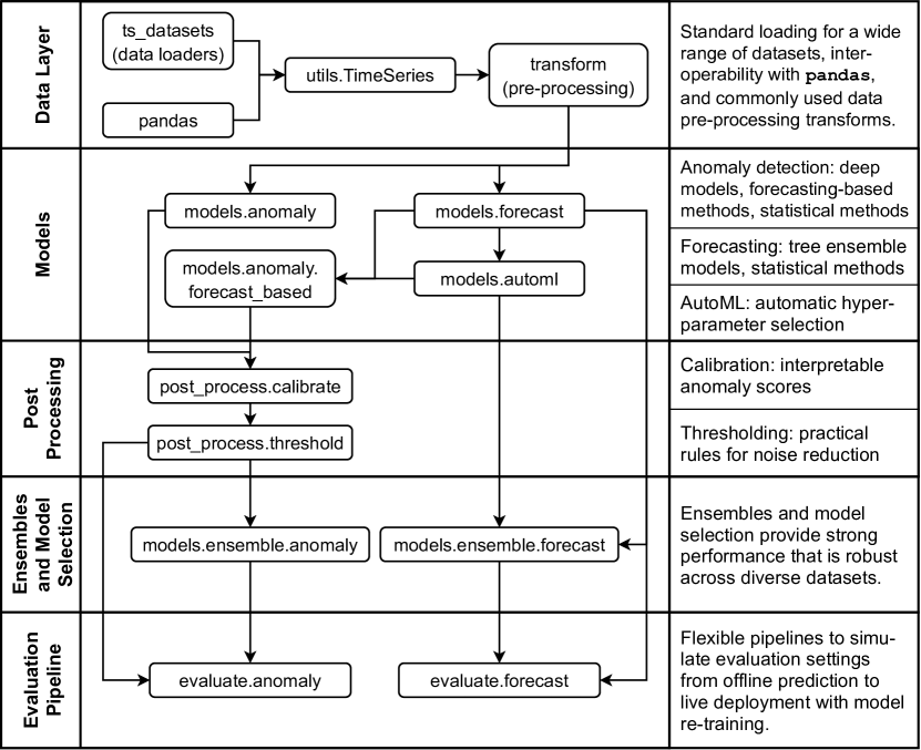
Figure 1: Architecture of modules in Merlion.

At a high level, Merlion’s module architecture is split into five layers: the data layer loads raw data, converts it to Merlion’s TimeSeries data structure, and performs any desired pre-processing; the modeling layer supports a wide array of models for both forecasting and anomaly detection, including autoML for automated hyperparameter tuning; the post-processing layer provides practical solutions to improve the interpetability and reduce the false positive rate of anomaly detection models; the next ensemble layer supports transparent model combination and model selection; and the final evaluation layer implements relevant evaluation metrics and pipelines that simulate the live deployment of a model in production. Figure 1 provides a visual overview of the relationships between these modules.

2.1 Data Layer

Merlion’s core data structure is the TimeSeries, which represents a generic multivariate time series $T$ as a collection of UnivariateTimeSeries $U^{(1)},\ldots,U^{(d)}$, where each UnivariateTimeSeries is a sequence $U^{(i)}=(t_{1}^{(i)},x_{1}^{(i)}),\ldots,(t_{n_{i}}^{(i)},x_{n_{i}}^{(i)})$. This formulation reflects the reality that individual univariates may be sampled at different rates, or contain missing data at different timestamps. For example, a cloud computing system may report its CPU usage every 10 seconds, but only report the amount of free disk space once per minute.

We allow users to initialize TimeSeries objects directly from pandas dataframes, and we implement standardized loaders for a wide range of datasets in the ts_datasets package.

Once a TimeSeries has been initialized from raw data, the merlion.transform module supports a host of pre-processing operations that can be applied before passing a TimeSeries to a model. These include resampling, normalization, moving averages, temporal differencing, and others. Notably, multiple transforms can be composed with each other (e.g. resampling followed by a moving average), and transforms can be inverted (e.g. the normalization $f(x)=(x-\mu)/\sigma$ is inverted as $f^{-1}(y)=\sigma y+\mu$).

2.2 Models

Since no single model can perform well across all time series and all use cases, it is important to provide users the flexibility to choose from a broad suite of heterogenous models. Merlion implements many diverse models for both forecasting and anomaly detection. These include statistical methods, tree-based models, and deep learning approaches, among others. To transparently expose all these options to an end user, we unify all Merlion models under two common API’s, one for forecasting, and one for anomaly detection. All models are initialized with a config object that contains implementation-specific hyperparameters, and support a model.train(time_series) method.

Given a general multivariate time series $T=(U^{(1)},\ldots,U^{(d)})$, forecasters are trained to predict the values of a single target univariate $U^{(k)}$. One can then obtain a model’s forecast of $U^{(k)}$ for a set of future time stamps by calling model.forecast(time_stamps).

Analogously, one can obtain an anomaly detector’s sequence of anomaly scores for the time series $T$ by simply calling model.get_anomaly_score(time_series). The handling of univariate vs. multivariate time series is implementation-specific (e.g. some algorithms look for an anomaly in any of the univariates, while others may look for anomalies in specific univariates). Notably, forecasters can also be used for anomaly detection by treating the residual between the true and predicted value of a target univariate $U^{(k)}$ as an anomaly score. These forecast-based anomaly detectors support both model.forecast(time_stamps) and model.get_anomaly_score(time_series).

For models that require additional computation, we implement a Layer interface that is the basis for the autoML features we offer. Layer is used to implement additional logic on top of existing model definitions that would not be properly fitted into the model code itself. Examples include seasonality detection and hyperparameter tuning (see §3.2 for more details). The Layer is an interface that implements three methods: generate_theta for generating hyperparameter candidates $\theta$, evaluate_theta for evaluating the quality of $\theta$’s, and set_theta for applying the chosen $\theta$ to the underlying model. A separate class ForecasterAutoMLBase implements forecast and train methods that leverage methods from the Layer class to complete the forecasting model.

Finally, all models support the ability to condition their predictions on historical data time_series_prev that is distinct from the data used for training. One can obtain these conditional predictions by calling model.forecast(time_stamps, time_series_prev) or model.get_anomaly_score(time_series, time_series_prev).

2.3 Post-Processing

All anomaly detectors have a post_rule which applies important post-processing to the output of model.get_anomaly_score(time_series). This includes calibration (§4.2.1), which ensures that anomaly scores correspond to standard deviation units and are therefore interpretable and consistent between different models, and thresholding (§4.2.2) rules to reduce the number of false positives. One can directly obtain post-processed anomaly scores by calling model.get_anomaly_label(time_series).

2.4 Ensembles and Model Selection

Ensembles are structured as a model that represents a combination of multiple underlying models. For this purpose we have a base EnsembleBase class that abstracts the process of obtaining predictions $Y_{1},\ldots,Y_{m}$ from $m$ underlying models on a single time series $T$, and a Combiner class that then combines results $Y_{1},\ldots,Y_{m}$ into the output of the ensemble. These combinations include traditional mean ensembles, as well as model selection based on evaluation metrics like sMAPE. Concrete implementations implement the forecast or get_anomaly_score methods on top of the tools provided by EnsembleBase, and their train method automatically handles dividing the data into train and validation splits if needed (e.g. for model selection).

2.5 Evaluation Pipeline

When a time series model is deployed live in production, training and inference are usually not performed in batch on a full time series. Rather, the model is re-trained at a regular cadence, and where possible, inference is performed in a streaming mode. To more realistically simulate this setting, we provide a EvaluatorBase class which implements the following evaluation loop:

1. Train an initial model on recent historical training data.

2. At a regular interval (e.g. once per day), retrain the entire model on the most recent data. This can be either the entire history, or a more limited window (e.g. 4 weeks).

3. Obtain the model’s predictions (forecasts or anomaly scores) for the time series values that occur between re-trainings. Users may customize whether this should be done in batch, streaming, or at some intermediate cadence.

4. Compare the model’s predictions against the ground truth (actual values for forecasting, or labeled anomalies for anomaly detection), and report quantitative evaluation metrics.

We also provide a wide range of evaluation metrics for both forecasting and anomaly detection, implemented as the enums ForecastMetric and TSADMetric, respectively. Finally, we provide scripts benchmark_forecast.py and benchmark_anomaly.py which allow users to use this logic to easily evaluate model performance on any dataset included in the ts_datasets module. We report experimental results using these scripts in §5.

3 Time Series Forecasting

In this section, we introduce Merlion’s specific univariate and multivariate forecasting models, provide algorithmic details on Merlion’s autoML and ensembling modules for forecasting, and describe the metrics used for experimental evaluation in §5.1 and §5.2.

3.1 Models

Merlion contains a number of models for univariate time series forecasting. These include classic statistcal methods like ARIMA (AutoRegressive Integrated Moving Average), SARIMA (Seasonal ARIMA) and ETS (Error, Trend, Seasonality), more recent algorithms like Prophet (Taylor and Letham, 2017), our previous production algorithm MSES (Cassius et al., 2021), and a deep autoregressive LSTM (Hochreiter and Schmidhuber, 1997), among others.

The multivariate forecasting models we use are based on autoregression and tree ensemble algorithms. For the autoregression algorithm, we adopt the Vector Autoregression model (VAR, Lütkepohl (2005)) that captures the relationship between multiple sequences as they change over time. For tree ensembles, we consider Random Forest (RF, Ho (1995)) and Gradient Boosting (GB, Ke et al. (2017)) as the base models. However, without appropriate modifications, tree ensemble models can be unsuitable for the general practice of time series forecasting. First, their output is a fixed-length vector, so it is not straightforward to obtain their forecasts for arbitrary prediction horizons. Second, these multivariate forecasting models often have incompatible data workflows or APIs that make it difficult to directly apply them for univariate prediction.

To overcome these obstacles, we propose an autoregressive forecasting strategy for our tree ensemble models, RF Forecaster and GB Forecaster. For a $d$-variable time series, these models forecast the value of all $d$ variables in the time series for time $t_{k}$, and they condition on this prediction to autoregressively forecast for time $t_{k+1}$. We thus enable these models to produce a forecast for an arbitrary prediction horizon, similar to more traditional models like VAR. Additionally, all our multivariate forecasting models share common APIs with the univariate forecasting models, and are therefore universal for both the univariate and the multivariate forecasting tasks. A full list of supported models can be found in the API documentation.

3.2 AutoML and Model Selection

The AutoML module for time series forecasting models is slightly different from autoML for coventional machine learning models, as we consider not only conventional hyper-parameter optimization, but also the detection of some characteristics of time series. Take the $\mathrm{SARIMA}(p,d,q)\times(P,Q,D)_{m}$ model as an example. Its hyperparameters include the autoregressive parameter $p$, difference order $d$, moving average parameter $q$, seasonal autoregressive parameter $P$, seasonal difference order $D$, seasonal moving average parameter $Q$, and seasonality $m$. While we use SARIMA as a motivating example, note that automatic seasonality detection can directly enhance other models like ETS and Prophet (Taylor and Letham, 2017). Meanwhile, choosing the appropriate (seasonal) difference order can yield a representation of the time series that makes the prediction task easier for any model.

Typically, we first analyze the time series to choose the seasonality $m$. Following the idea from the theta method (Assimakopoulos and Nikolopoulos, 2000), we say that a time series has seasonality $m$ at significance level $a$ if

$$|r_{m}|>\Phi^{-1}(1-a/2)\sqrt{\frac{1+2\sum^{m-1}_{i=1}r_{i}^{2}}{n}},$$

where $r_{k}$ is the lag-$k$ autocorrelation, $m$ is the number of periods within a seasonal cycle, $n$ is the sample size, and $\Phi^{-1}$ is the quantile function of the standard normal distribution. By default, we set the significance at $a=0.05$ to reflect the 95% prediction intervals.

Next, we select the seasonal difference order $D$ by estimating the strength of the seasonal component with the time series decomposition method (Cleveland et al., 1990). Suppose the time series can be written as $y=T+S+R$, where $T$ is the smoothed trend component, $S$ is the seasonal component and $R$ is the remainder. Then, the strength of the seasonality (Wang et al., 2006) is

$$F_{S}=\max\left(0,1-\frac{\mathrm{Var}(R)}{\mathrm{Var}(S+R)}\right).$$

Note that a time series with strong seasonality will have $F_{S}$ close to $1$ since $\mathrm{Var}(R)$ is much smaller than $\mathrm{Var}(S+R)$. If $F_{S}$ is large, we adopt the seasonal difference operation. Thus, we choose $D$ by successviely decomposing the time series and differencing it based on the detected seasonality until $F_{S}$ is relatively small. We can then choose the difference order $d$ by applying successive KPSS unit-root tests to the seasonally differenced data.

Once $m$, $D$, and $d$ are selected, we can choose the remaining hyperparameters $p$, $q$, $P$, and $Q$ by minimizing the AIC (Akaike Information Criterion) via grid search. Because the parameter space is exponentially large if we exhastively enumerate all the hyperparameter combinations, we follow the step-wise search method of Hyndman and Khandakar (2008). To further speed up the training time of the autoML module, we propose the following approximation strategy: we obtain an initial list of candidate models that achieve good performance after relatively few optimization iterations; we then re-train each of these candidates until model convergence, and finally select the best model by AIC.

3.3 Ensembles

Ensembles of forecasters in Merlion allow a user to transparently combine models in two ways. First, we support traditional ensembles that report the mean or median value predicted by all the models at each timestamp. Second, we support automated model selection. When performing model selection, we divide the training data into train and validation splits, train each model on the training split, and obtain its predictions for the validation split. We then evaluate the quality of those predictions using a user-specified evaluation metric like sMAPE or RMSE (§3.4), and return the model that achieved the best performance after re-training it on the full training data. These features are useful in many practical scenarios, as they can greatly reduce the amount of human intervention needed when deploying a model.

3.4 Evaluation Metrics

There are many ways to evaluate the accuracy of a forecasting model. Given a time series with $n$ observations, let $y_{t}$ denote the observed value at time $t$ and $\hat{y}_{t}$ denote the corresponding predicted value. Then the forecasting error $e_{t}$ at time $t$ is $y_{t}-\hat{y}_{t}$. Error measures based on absolute or squared errors are widely used, and they are formuated as

$$\text{MAE}=\frac{1}{n}\sum^{n}_{t=1}|e_{t}|\quad\text{and}\quad\text{RMSE}=\sqrt{\frac{\sum^{n}_{t=1}e_{t}^{2}}{n}},$$

respectively. Unfortunately, these measures cannot be compared across time series that are on different scales. To achive scale-independence, one alternative approach is to use percentage errors based on the observed values. One typical measure is sMAPE (Makridakis and Hibon, 2000), defined as:

$$\text{sMAPE}=\frac{1}{n}\sum^{n}_{t=1}\frac{|e_{t}|}{|y_{t}|+|\hat{y}_{t}|}*200(\%),$$

Unfortunately, sMAPE has the disadvantage of being ill-defined if $y_{t}$ and $\hat{y}_{t}$ are both close to zero. To address this issue, one alternative measure is MARRE, which is defined as

$$\text{MARRE}=\frac{1}{n}\frac{\sum^{n}_{t=1}|e_{t}|}{|\max(y_{t})-\min(y_{t})|}.$$

However, MARRE is not always suitable for non-stationary time series, where the scale of the data may evolve over time. Merlion’s ForecastMetric enum supports all the above classes of evaluation metrics, as well as others detailed in the API documentation. By default, we evaluate forecasting results by sMAPE, but users may manually specify alternatives if their application calls for it.

4 Time Series Anomaly Detection

In this section, we introduce Merlion’s specific univariate and multivariate anomaly detection models, provide algorithmic details on Merlion’s post-processing and ensembling modules for anomaly detection, and describe the metrics used for experimental evaluation in §5.3 and §5.4.

4.1 Models

Merlion contains a number of models that are specialized for univariate time series anomaly detection. These fall into two groups: forecasting-based and statistical. Because forecasters in Merlion predict the value of a specific univariate in a general time series, they are straightforward to adapt for anomaly detection. The anomaly score is simply the residual between the predicted and true time series value, optionally normalized by the underlying forecaster’s predicted standard error (if it produces one).

For univariate statistical methods, we support Spectral Residual (Ren et al., 2019), as well as two simple baselines WindStats and ZMS. WindStats divides each week into windows (e.g. 6 hours), and computes the anomaly score $s_{t}=(x_{t}-\mu(t))/\sigma(t)$, where $\mu(t)$ and $\sigma(t)$ are the historical mean and standard deviation of the window in question (e.g. 12pm to 6pm on Monday). ZMS computes $k$-lags $\Delta^{(k)}_{t}=x_{t}-x_{t-k}$ for $k=1,2,4,8,\ldots$, and computes the anomaly score $s_{t}=\max_{k}(\Delta^{(k)}_{t}-\mu^{(k)})/\sigma^{(k)}$, where $\mu^{(k)}$ and $\sigma^{(k)}$ are the mean and standard deviation of each $k$-lag.

In addition to models that are specialized for univariate anomaly detection, we support both statistical methods and deep learning models that can handle both univariate and multivariate anomaly detection. The statistical methods include Isolation Forest (Liu et al., 2008) and Random Cut Forest Guha et al. (2016), while the deep learning models include an autoencoder (Baldi, 2012), a Deep Autoencoding Gaussian Mixture Model (DAGMM, Zong et al. (2018)), a LSTM encoder-decoder (Sutskever et al., 2014), and a variational autoencoder (Kingma and Welling, 2013). A full list can be found in the API documentation.

4.2 Post-Processing

Merlion supports two key post-processing steps for anomaly detectors: calibration and thresholding. Calibration is important for improving model intepretability, while thresholding converts a sequence of continuous anomaly scores into discrete labels and reduces the false positive rate.

4.2.1 Calibration

All anomaly detectors in Merlion return anomaly scores $s_{t}$ such that $\absolutevalue{s_{t}}$ is positively correlated with the severity of the anomaly. However, the scales and distributions of these anomaly scores vary widely. For example, Isolation Forest (Liu et al., 2008) returns an anomaly score $s_{t}\in[0,1]$ where $-\log_{2}(1-s_{t})$ is a node’s depth in a binary tree; Spectral Residual (Ren et al., 2019) returns an unnormalized saliency map; DAGMM (Zong et al., 2018) returns a negative log probability.

To successfully use a model, one must be able to interpret the anomaly scores it returns. However, this prevents many models from being immediately useful to users who are unfamiliar with their specifc implementations. Calibration bridges this gap by making all anomaly scores interpretable as z-scores, i.e. values drawn from a standard normal distribution.

Let $\Phi:\mathbb{R}\to[0,1]$ be the cumulative distribution function (CDF) of the standard normal distribution. A calibrator $C:\mathbb{R}\to\mathbb{R}$ converts a raw anomaly score $s_{t}$ into a calibrated score $z_{t}$ such that $\mathbb{P}[\absolutevalue{z_{t}}>\alpha]=\Phi(\alpha)-\Phi(-\alpha)=2\Phi(\alpha)-1$, i.e. $\absolutevalue{z_{t}}$ follows the same distribution as the absolute value of a standard normal random variable. If $F_{s}:\mathbb{R}\to[0,1]$ is the CDF of the absolute raw anomaly scores $\absolutevalue{s_{t}}$, we can compute the recalibrated score as

$$C(s_{t})=\mathrm{sign}(s_{t})\Phi^{-1}((1+F_{s}(\absolutevalue{s_{t}}))/2)$$

Notably, this is also the optimal transport map between the two distributions, i.e. the mapping which transfers mass from one distribution to the other in a way that minimizes the $\ell_{1}$ transportation cost (Villani, 2003).

In practice, we estimate the calibration function $C$ using the empirical CDF $\hat{F}_{s}$ and a monotone spline interpolator (Fritsch and Butland, 1984) for intermediate values. This simple post-processing step dramatically increases the intepretability of the anomaly scores returned by individual models. It also enables us to create ensembles of diverse anomaly detectors as discussed in §4.3. This functionality is enabled by default for all anomaly detection models.

4.2.2 Thresholding

The most common way to decide whether an individual timestamp $t$ as anomalous, is to compare the anomaly score $s_{t}$ against a threshold $\tau$. However, in many real-world systems, a human is alerted every time an anomaly is detected. A high false positive rate will lead to fatigue from the end users who have to investigate each alert, and may result in a system whose users think it is unreliable.

A common way to circumvent this problem is including additional automated checks that must pass before a human is alerted. For instance, our system may only fire an alert if there are two timestamps $t_{1},t_{2}$ within a short window (e.g. 1 hour) with a high anomaly score, i.e. $\absolutevalue{s_{t_{1}}}>\tau$ and $\absolutevalue{s_{t_{2}}}>\tau$. Moreover, if we know that anomalies typically last 2 hours, our system can simply suppress all alerts occurring within 2 hours of a recent one, as those alerts likely correspond to the same underlying incident. Often, one or both of these steps can greatly increase precision without adversely impacting recall. As such, they are commonplace in production systems.

Merlion implements all these features in the user-configurable AggregateAlarms post-processing rule, and by default, it is enabled for all anomaly detection models.

4.3 Ensembles

Because both time series and the anomalies they contain are incredibly diverse, it is unlikely that a single model will be the best for all use cases. In principle, a heterogenous ensemble of models may generalize better than any individual model in that ensemble. Unfortunately, as mentioned in §4.2.1, constructing an ensemble is not straightforward due to the vast differences in anomaly scores returned by various models.

However, because we can rely on the anomaly scores of all Merlion models to be interpretable as z-scores, we can construct an ensemble of anomaly detectors by simply reporting the mean calibrated anomaly score returned by each individual model, and then applying a threshold (a la §4.2.2) on this combined anomaly score. Empirically, we find that ensembles robustly achieve the strongest or competitive performance (relative to the baselines considered) across multiple open source and internal datasets for both univariate (Table 10) and multivariate (Table 13) anomaly detection.

4.4 Evaluation Metrics

The key challenge in designing an appropriate evaluation metric for time series anomaly detection lies in the fact that anomalies are almost always windows of time, rather than discrete points. Thus, while it is easy to compute the pointwise (PW) precision, recall, and F1 score of a predicted anomaly label sequence relative to the ground truth label sequence, these metrics do not reflect a quantity that human operators care about.

Xu et al. (2018) propose point-adjusted (PA) metrics as a solution to this problem: if any point in a ground truth anomaly window is labeled as anomalous, all points in the segment are treated as true positives. If no anomalies are flagged in the window, all points are labeled as false negatives. Any predicted anomalies outside of anomalous windows are treated as false positives. Precision, recall, and F1 can be computed based on these adjusted true/false positive/negative counts. However, the disadvantage of PA metrics is that they are biased to reward models for detecting long anomalies more than short ones.

Hundman et al. (2018) propose revised point-adjusted (RPA) metrics as a closely related alternative: if any point in a ground truth anomaly window is labeled as anomalous, one true positive is registered. If no anomalies are flagged in the window, one false negative is recorded. Any predicted anomalies outside of anomalous windows are treated as false positives. These metrics address the shortcomings of PA metrics, but they do penalize false positives more heavily than alternatives.

Merlion’s TSADMetric enum supports all 3 classes of evaluation metrics (PW, PA, and RPA), as well as the mean time to detect an anomaly. By default, we evaluate RPA metrics, but users may manually specify alternatives if their application calls for it.

5 Experiments

In the experiments section, we show benchmark results generated by using Merlion with popular baseline models across several time series datasets. The purpose of this section is not to obtain state-of-the-art results. Rather, most algorithms listed are strong baselines. To avoid the possible risk of label leaking through manual hyperparameter tuning, for all experiments, we evaluate all models with a single choice of sensible default hyperparameters and data pre-processing, regardless of dataset.

5.1 Univariate Forecasting

5.1.1 Datasets and Evaluation

We primarily evaluate our models on the M4 benchmark (Makridakis et al., 2018, 2020), an influential time series forecasting competition. The dataset contains $100,000$ time series from diverse domains including financial, industry, and demographic forecasting. It has sampling frequencies ranging from hourly to yearly. Table 2 summarizes the dataset. We additionally evaluate on three internal datasets of cloud KPIs, which we describe in Table 3. For all datasets, models are trained and evaluated in the offline batch prediction setting, with a pre-defined prediction horizon equal to the size of the test split. To mitigate the effect of outliers, we report both the mean and median sMAPE for each method.

M4	Hourly	Daily	Weekly	Monthly	Quarterly	Yearly
# Time Series	414	4,227	359	48,000	24,000	23,000
Real Data?	✓	✓	✓	✓	✓	✓
Availability	Public	Public	Public	Public	Public	Public
Prediction Horizon	6	8	18	13	14	48

Table 2: Summary of M4 dataset for univariate forecasting.

	Int_UF1	Int_UF2	Int_UF3
# Time Series	21	6	4
Real Data?	✓	✓	✓
Availability	Internal	Internal	Internal
Train Split	First 75%	First 25%	First 25%

Table 3: Summary of internal datasets for univariate forecasting.

5.1.2 Models

We compare ARIMA (AutoRegressive Integrated Moving Average), Prophet (Taylor and Letham, 2017), ETS (Error, Trend, Seasonality), and MSES (the previous production solution, Cassius et al. (2021)). For ARIMA, Prophet and ETS, we also consider our autoML variants that perform automatic seasonality detection and hyperparameter tuning, as described in §3.2. These are implemented using the merlion.models.automl module.

	M4$\_$Hourly		M4$\_$Daily		M4$\_$Weekly
sMAPE	Mean	Median	Mean	Median	Mean	Median
MSES	32.45	16.89	5.87	3.97	16.53	9.96
ARIMA	33.54	19.27	3.23	2.06	9.29	5.38
Prophet	18.08	6.92	11.67	5.99	19.98	11.26
ETS	42.95	19.88	3.04	2.00	9.00	5.17
AutoSARIMA	13.61	4.73	3.29	2.00	8.30	5.09
AutoProphet	16.49	6.20	11.67	5.98	20.01	11.63
AutoETS	19.23	5.33	3.07	1.98	9.32	5.15

	M4$\_$Monthly		M4$\_$Quarterly		M4$\_$Yearly
sMAPE	Mean	Median	Mean	Median	Mean	Median
MSES	25.40	13.69	19.03	9.53	21.63	12.11
ARIMA	17.66	10.41	13.37	8.27	16.37	10.34
Prophet	20.64	11.00	24.53	12.81	30.23	19.24
ETS	14.32	8.37	11.08	6.94	16.43	11.43
AutoSARIMA	14.26	7.17	10.51	5.44	17.16	9.48
AutoProphet	20.43	10.42	24.62	12.87	30.23	19.24
AutoETS	13.73	7.41	10.33	5.77	15.96	9.18

Table 4: Mean and Median sMAPE achived by univariate forecasting models on M4 datasets. All models were evaluated without retraining. Best results are in bold.

	Int_UF1		Int_UF2		Int_UF3
sMAPE	Mean	Median	Mean	Median	Mean	Median
MSES	33.50	32.60	32.30	14.45	3.882	3.771
ARIMA	24.00	19.42	25.89	24.40	5.94	6.15
Prophet	56.07	42.10	30.93	38.54	72.55	78.27
ETS	17.02	16.36	25.10	24.19	3.55	3.32
AutoSARIMA	15.98	15.10	17.45	9.98	3.42	3.41
AutoProphet	56.43	41.99	26.35	24.19	69.32	78.37
AutoETS	21.65	20.15	19.41	12.67	3.15	2.94

Table 5: Mean and Median sMAPE achived by univariate forecasting models on internal datasets. All models were evaluated without retraining. Best results are in bold.

ARIMA $\to$ AutoSARIMA	$5.03$ ($p=0.010$)
Prophet $\to$ AutoProphet	$1.01$ ($p=0.035$)
ETS $\to$ AutoETS	$2.96$ ($p=0.039$)

Table 6: Average reduction (improvment) in sMAPE achieved by applying autoML. $p$-value is from a 2-sided paired sample $t$-test. Our autoML module improves all 3 models at significance level $p=0.05$.

5.1.3 Results

Table 4 and 5 respectively show the performance of each model on the public and internal datasets. Table 6 shows the average improvement achieved by using the autoML module. For ARIMA, we find a clear improvement by using the AutoML module for all datasets. While the improvement is statistically significant for Prophet and AutoETS overall, the actual change is small on most datasets except M4_Hourly and Int_UF2. This is because many of the other datasets don’t contain well-defined seasonalities; additionally, Prophet already has some pre-defined seasonality detection (daily, weekly, and yearly), but these datasets contain time series with hourly seasonalities.

While there is no clear winner across all datasets, AutoSarima and AutoETS consistently outperform other methods. The overall performance of AutoSarima is slightly better than AutoETS, but AutoSarima is much slower to train. Therefore, we believe that AutoETS is a good “default” model for new users or early exploration.

5.2 Multivariate Forecasting

5.2.1 Datasets and Evaluation

	Power Grid	Seattle Trail	Solar Plant	Int_MF
# Time Series	1	1	1	21
# Variables	10	5	405	22
Real Data?	✓	✓	✓	✓
Availability	Public	Public	Public	Internal
Data Source	Energy Demand	Trail Traffic	Power Generation	Cloud KPIs
Train Split	First 70%	First 70%	First 70%	First 75%
Granularity	1h	✗	30min	10s
Reference	ene (2018)	sea (2018)	Shih et al. (2019)	–

Table 7: Summary of multivariate forecasting datasets.

We collect public and internal datasets (Table 7) and train models on a training split of the data. For some datasets, we resample the data with given granularities. For each time series, we train the models on the training split to predict the first univariate as a target sequence. While we don’t re-train the model, we use the evaluation pipeline described in §2.5 to incrementally obtain predictions for the test split using a rolling window. We predict time series values for the next 3 timestamps, while conditioning the prediction on the previous 21 timestamps. We obtain these 3-step predictions at every timestamp in the test split, and evaluate the quality of the prediction using sMAPE where possible, and RMSE otherwise.

5.2.2 Models

The multivariate forecasting models we use are based on the autoregression and tree ensemble algorithms. We compare VAR (Lütkepohl, 2005), GB Forecaster based on the Gradient Boosting algorithm (Ke et al., 2017) and RF Forecaster based on the Random Forest algorithm (Ho, 1995). We discuss the implementation details of these models in §3.1. For the GB Forecster and RF Forecaster, we use our proposed autoregression strategy to enable them to forecast for an arbitrary prediction horizon.

5.2.3 Results

Table 8 reports the performance of each model. We find that our proposed autogression-based tree ensemble model GB Forecaster achieves the best results on three of the four datasets and is competitive with the best result on the fourth. While the VAR model shows competitive performance on some datasets, it is not as robust. For example, the Seattle Trail dataset has large outliers (several orders of magnitude larger than the mean) that dramatically impact the performance of VAR. For this reason, we believe that GB Forecaster is a good “default” model for new users or early exploration.

	Power Grid	Seattle Trail	Solar Plant	Int_MF
	sMAPE	RMSE	RMSE	sMAPE	sMAPE
	(1 TS)	(1 TS)	(1 TS)	(mean)	(median)
VAR	1.131	968048	10.30	22.11	17.87
GB Forecaster	1.705	41.66	3.712	14.05	12.18
RF Forecaster	3.256	44.20	4.633	23.25	19.82

Table 8: Performance of multivariate forecasting models. All models were evaluated without retraining. Best results are in bold. We report RMSE instead of sMAPE for the Seattle Trail and Solar Plant datasets because a large portion of the data values (13% and 55% respectively) are equal to 0, making them unsuitable for sMAPE. 1 TS means that there is only one time series in the dataset.

5.3 Univariate Anomaly Detection

5.3.1 Datasets and Evaluation

	Int_UA	NAB	AIOps	UCR
# Time Series	26	58	29	250
Real data?	✓	47/58 real	✓	Mixed
Availability	Internal	Public	Public	Public
Data Source	Cloud KPIs	Various	Cloud KPIs	Various
Train split	First 25%	First 15%	First 50%	First 30%
Supervised?	No	No	Train labels	Test labels
Threshold	4.0	3.5	–	–
Reference	–	Lavin and Ahmad (2015)	aio (2018)	Dau et al. (2018)

Table 9: Summary of univariate anomaly detection datasets.

We report results on four public and internal datasets (Table 9). For the internal dataset and the Numenta Anomaly Benchmark (NAB, Lavin and Ahmad (2015)), we choose a single (calibrated) detection threshold for all time series and all algorithms. For the AIOps challenge (aio, 2018), we use the labeled anomalies in the training split of each time series to choose the detection threshold that optimizes F1 on the training split; for the UC Riverside Time Series Anomaly Archive (Dau et al., 2018), we choose the detection threshold that optimizes F1 on the test split. This is because the dataset is incredibly diverse (so a single threshold doesn’t apply to all time series), and there are no anomalies present in the training split. Table 9 summarizes these datasets and evaluation choices.

We use the evaluation pipeline described in §2.5 to evaluate each model. After training an initial model on the training split of a time series, we re-train the model unsupervised either daily or hourly on the full data until that point (without adjusting the calibrator or threshold). We then incrementally obtain predicted anomaly scores for the full time series, in a way that simulates a live deployment scenario. We also consider batch prediction, where the initial trained model predicts anomaly scores for the entire test split in a single step, without any re-training. Note that the UCR dataset does not contain timestamps; we treat it as if it is sampled once per minute, but this is an imperfect assumption. We consider only batch prediction and “daily” retraining for this dataset for efficiency reasons.

5.3.2 Models

We evaluate two classes of models: forecast-based anomaly detectors and statistical methods. For forecast-based methods, we use ARIMA, AutoETS, and AutoProphet (as described in §5.1). For statistical methods, we use Isolation Forest (Liu et al., 2008), Random Cut Forest (Guha et al., 2016), and Spectral Residual (Ren et al., 2019), as well as two simple baselines WindStats and ZMS (§4.1). We also consider an ensemble of AutoETS, RRCF, and ZMS (using the algorithm described in §4.3).

5.3.3 Results

	Int_UA	NAB	AIOps	UCR	$\Delta$ F1 (vs. best)
ARIMA	$\bm{0.531}$	$0.395$	$0.227$	$0.313$	$0.148\pm 0.099$
AutoETS	$0.296$	$0.350$	$0.097$	$0.334$	$0.245\pm 0.042$
AutoProphet	$0.343$	$0.323$	$0.310$	$0.418$	$0.166\pm 0.062$
Isolation Forest	$0.436$	$0.244$	$0.347$	$0.461$	$0.142\pm 0.111$
Random Cut Forest	$0.248$	$0.337$	$0.314$	$\bm{0.568}$	$0.148\pm 0.132$
Spectral Residual	$0.340$	$0.153$	$0.338$	$0.469$	$0.189\pm 0.150$
WindStats (baseline)	$0.225$	$0.247$	$0.324$	$0.306$	$0.239\pm 0.114$
ZMS (baseline)	$0.486$	$0.290$	$0.340$	$0.427$	$0.129\pm 0.094$
Ensemble (ours)	$0.500$	$\bm{0.548}$	$\bm{0.396}$	$0.476$	$\bm{0.034\pm 0.044}$

Table 10: F1 scores achieved by univariate anomaly detection models. All models were evaluated using batch prediction, daily re-training, and hourly re-training; we report the best F1 achieved by any of the re-training schedules. We also report the average gap (over datasets) in F1 between each model and the best model. Best results are in bold.

	Daily	Hourly
ARIMA	$0.162$ ($p=0.001$)	$0.227$ ($p<0.001$)
AutoETS	$0.088$ ($p=0.017$)	$0.058$ ($p=0.325$)
AutoProphet	$0.028$ ($p=0.013$)	–
Isolation Forest	$0.006$ ($p=0.779$)	$0.019$ ($p=0.567$)
Random Cut Forest	$0.024$ ($p=0.396$)	$0.033$ ($p=0.337$)
Spectral Residual	$-0.090$ ($p=0.075$)	$-0.109$ ($p=0.004$)
WindStats (baseline)	$0.044$ ($p=0.098$)	$0.017$ ($p=0.145$)
ZMS (baseline)	$0.005$ ($p=0.929$)	$0.011$ ($p=0.872$)
Ensemble (ours)	$0.147$ ($p=0.023$)	$0.183$ ($p=0.009$)

Table 11: Average change in F1 (relative to no re-training) achieved by re-training models both daily and hourly. $p$-value is from a 2-sided paired sample $t$-test. Re-training makes a significant improvement for the forecasting models (first block) and the ensemble. However, the statistical models (second block) benefit only marginally (if at all).

Table 10 reports the revised point-adjusted F1 score achieved by each model on each dataset. We report the best F1 score achieved by any of the 3 re-training schedules (for efficiency reasons, we only consider batch prediction and daily re-training for AutoProphet). We find that our proposed ensemble of AutoETS, RRCF, and ZMS achieves the best performance on two of the four datasets, and the second-best on the others; overall, it has the smallest average gap in F1 score relative to the best model for each dataset (along with the smallest variance in this gap). For this reason, we believe that it is a good “default” model for new users or early exploration.

Table 11 examines the impact of the re-training schedule for each model, averaged across all datasets. We find that daily and hourly re-training of forecasting-based models and our proposed ensemble can greatly improve their anomaly detection performance. However, in practice, the ideal re-training frequency may require some experimentation to choose. Interestingly, the impact of frequent re-training is unclear for most statistical models.

5.4 Multivariate Anomaly Detection

5.4.1 Datasets and Evaluation

The evaluation setting for multivariate anomaly detection is nearly identical to that for univariate anomaly detection. Table 12 describes the multivariate time series anomaly detection datasets in this epxeriment. Note that we treat anomaly detection on all these datasets as a fully unsupervised learning task. The main difference from the univariate setting is that we consider only batch predictions and weekly retraining (rather than batch predictions, daily re-training, and hourly retraining) for efficiency reasons.

	SMD	SMAP	MSL	Int_MA
# Time Series	28	1	1	20
# Variables	38	25	55	5
Real data?	✓	✓	✓	✓
Availability	Public	Public	Public	Internal
Data Source	Cloud KPIs	Satellite Data	Mars Rover	Cloud KPIs
Train split	First 50%	First 25%	First 45%	First 50%
Supervised?	No	No	No	No
Threshold	3.0	3.5	3.0	3.5
Reference	Su et al. (2019)	Hundman et al. (2018)	Hundman et al. (2018)	–

Table 12: Summary of multivariate anomaly detection datasets.

5.4.2 Models

We consider two classes of models: statistical methods and deep learning models. For statistical methods, we evaluate Isolation Forest (Liu et al., 2008) and Random Cut Forest (Guha et al., 2016) as in §5.3. For deep learning approaches, we evaluate an autoencoder (Baldi, 2012), a Deep Autoencoding Gaussian Mixture Model (DAGMM, Zong et al. (2018)), a LSTM encoder-decoder (Sutskever et al., 2014), and a variational autoencoder (Kingma and Welling, 2013). We also consider an ensemble of a Random Cut Forest and a Variational Autoencoder (using the algorithm described in §4.3).

5.4.3 Results

	SMD	SMAP	MSL	Int_MA	$\Delta$ F1 (vs. best)
Isolation Forest	$0.388$	$0.211$	$0.226$	$0.252$	$0.129\pm 0.025$
Random Cut Forest	$\bm{0.500}$	$0.108$	$0.312$	$0.313$	$0.091\pm 0.110$
Autoencoder	$0.264$	$\bm{0.357}$	$0.355$	$\bm{0.357}$	$0.065\pm 0.114$
DAGMM	$0.191$	$0.037$	$0.135$	$0.182$	$0.262\pm 0.067$
LSTM Encoder-Decoder	$0.344$	$\bm{0.357}$	$\bm{0.381}$	$0.301$	$0.053\pm 0.074$
Variational Autoencoder	$0.318$	$0.187$	$\bm{0.381}$	$0.322$	$0.097\pm 0.093$
Ensemble (ours)	$0.403$	$0.291$	$0.357$	$0.341$	$\bm{0.051\pm 0.038}$

Table 13: F1 scores achieved by multivariate anomaly detection models. All models were evaluated using batch prediction and weekly re-training; we report the best F1 achieved by any of the re-training schedules. We also report the average gap (over datasets) in F1 between each model and the best model. Best results are in bold.

	Weekly
Isolation Forest	$0.006$ ($p=0.796$)
Random Cut Forest	$0.036$ ($p=0.130$)
Autoencoder	$-0.075$ ($p=0.352$)
DAGMM	$0.057$ ($p=0.032$)
LSTM Encoder-Decoder	$0.001$ ($p=0.970$)
Variational Autoencoder	$0.020$ ($p=0.286$)
Ensemble (ours)	$-0.032$ ($p=0.499$)

Table 14: Average change in F1 (relative to no re-training) achieved by re-training models weekly. $p$-value is from a 2-sided paired sample $t$-test. The changes are not statistically significant at $p=0.05$ for any models besides DAGMM.

Table 13 reports the revised point-adjusted F1 score achieved by each model. While there is no clear winner across all datasets, our proposed ensemble consistently achieves a small gap in F1 score relative to the best model for each dataset. The LSTM encoder-decoder achieves a similar average gap, but it has a larger variance. Therefore, we believe the ensemble to be a good “default” model for new users or early exploration, as it robustly obtains reasonable performance across multiple datasets. Finally, like the univariate case, Table 14 shows that the impact of re-training is ambiguous for all the multivariate statistical models considered (first block), as well as the deep learning models (second block).

6 Conclusion and Future Work

We introduce Merlion, an open source machine learning library for time series, which is designed to address many of the pain points in today’s industry workflows for time series anomaly detection and forecasting. It provides unified, easily extensible interfaces and implementations for a wide range of models and datasets, an autoML module that consistently improves the performance of multiple forecasting models, post-processing rules for anomaly detectors that improve interpretability and reduce the false positive rate, and transparent support for ensembles that robustly achieve good performance on multiple benchmark datasets. These features are tied together in a flexible pipeline that quantitatively evaluates the performance of a model and a visualization module for more qualitative analysis.

We continue to actively develop and improve Merlion. Planned future work includes adding support for more models including the latest deep learning models and online learning algorithms, developing a streaming platform to facilitate model deployment in a real production environment, and implementing advanced features for multivariate time series analysis. We welcome and encourage any contributions from the open source community.

References

- aio (2018) AIOps Challenge, 2018. URL http://iops.ai/competition_detail/?competition_id=5.
- ene (2018) Hourly energy consumption, 2018. URL https://www.kaggle.com/robikscube/hourly-energy-consumption/metadata.
- sea (2018) Seattle burke-gilman trail, 2018. URL https://www.kaggle.com/city-of-seattle/seattle-burke-gilman-trail/metadata.
- Alexandrov et al. (2020) Alexander Alexandrov, Konstantinos Benidis, Michael Bohlke-Schneider, Valentin Flunkert, Jan Gasthaus, Tim Januschowski, Danielle C. Maddix, Syama Rangapuram, David Salinas, Jasper Schulz, Lorenzo Stella, Ali Caner Türkmen, and Yuyang Wang. GluonTS: Probabilistic and Neural Time Series Modeling in Python. Journal of Machine Learning Research, 21(116):1–6, 2020. URL http://jmlr.org/papers/v21/19-820.html.
- Assimakopoulos and Nikolopoulos (2000) Vassilis Assimakopoulos and Konstantinos Nikolopoulos. The theta model: a decomposition approach to forecasting. International journal of forecasting, 16(4):521–530, 2000.
- Audibert et al. (2020) Julien Audibert, Pietro Michiardi, Frédéric Guyard, Sébastien Marti, and Maria A. Zuluaga. Usad: Unsupervised anomaly detection on multivariate time series. In The 26th ACM SIGKDD Intl Conference on Knowledge Discovery & Data Mining, KDD’20, page 3395–3404, 2020.
- Baldi (2012) Pierre Baldi. Autoencoders, unsupervised learning, and deep architectures. In Isabelle Guyon, Gideon Dror, Vincent Lemaire, Graham Taylor, and Daniel Silver, editors, Proceedings of ICML Workshop on Unsupervised and Transfer Learning, volume 27 of Proceedings of Machine Learning Research, pages 37–49, Bellevue, Washington, USA, 02 Jul 2012. PMLR. URL https://proceedings.mlr.press/v27/baldi12a.html.
- Cassius et al. (2021) Rowan Cassius, Arun Kumar Jagota, and Aadyot Bhatnagar. Multi-scale exponential smoother, 2021. URL https://salesforce.github.io/Merlion/merlion.models.forecast.html#module-merlion.models.forecast.smoother.
- Cleveland et al. (1990) Robert B Cleveland, William S Cleveland, Jean E McRae, and Irma Terpenning. Stl: A seasonal-trend decomposition. J. Off. Stat, 6(1):3–73, 1990.
- Dang et al. (2019) Yingnong Dang, Qingwei Lin, and Peng Huang. Aiops: real-world challenges and research innovations. In 2019 IEEE/ACM 41st International Conference on Software Engineering: Companion Proceedings (ICSE-Companion), pages 4–5. IEEE, 2019.
- Dau et al. (2018) Hoang Anh Dau, Eamonn Keogh, Kaveh Kamgar, Chin-Chia Michael Yeh, Yan Zhu, Shaghayegh Gharghabi, Chotirat Ann Ratanamahatana, Yanping, Bing Hu, Nurjahan Begum, Anthony Bagnall, Abdullah Mueen, Gustavo Batista, and Hexagon-ML. The ucr time series classification archive, October 2018. https://www.cs.ucr.edu/~eamonn/time_series_data_2018/.
- Fritsch and Butland (1984) F. N. Fritsch and J. Butland. A method for constructing local monotone piecewise cubic interpolants. SIAM Journal on Scientific and Statistical Computing, 5(2):300–304, June 1984. doi: 10.1137/0905021.
- Guha et al. (2016) Sudipto Guha, Nina Mishra, Gourav Roy, and Okke Schrijvers. Robust random cut forest based anomaly detection on streams. In Maria Florina Balcan and Kilian Q. Weinberger, editors, Proceedings of The 33rd International Conference on Machine Learning, volume 48 of Proceedings of Machine Learning Research, pages 2712–2721, New York, New York, USA, 20–22 Jun 2016. PMLR. URL https://proceedings.mlr.press/v48/guha16.html.
- Ho (1995) Tin Kam Ho. Random decision forests. In Proceedings of 3rd international conference on document analysis and recognition, volume 1, pages 278–282. IEEE, 1995.
- Hochreiter and Schmidhuber (1997) Sepp Hochreiter and Jürgen Schmidhuber. Long short-term memory. Neural Computation, 9(8):1735–1780, 1997. doi: 10.1162/neco.1997.9.8.1735.
- Hosseini et al. (2021) Reza Hosseini, Albert Chen, Kaixu Yang, Sayan Patra, and Rachit Arora. Greykite: a flexible, intuitive and fast forecasting library, 2021. URL https://github.com/linkedin/greykite.
- Hundman et al. (2018) Kyle Hundman, Valentino Constantinou, Christopher Laporte, Ian Colwell, and Tom Söderström. Detecting spacecraft anomalies using lstms and nonparametric dynamic thresholding. CoRR, abs/1802.04431, 2018. URL http://arxiv.org/abs/1802.04431.
- Hyndman and Khandakar (2008) Rob J Hyndman and Yeasmin Khandakar. Automatic time series forecasting: the forecast package for r. Journal of statistical software, 27(1):1–22, 2008.
- Jiang (2021) Xiaodong Jiang. Kats, 2021. URL https://github.com/facebookresearch/Kats.
- Ke et al. (2017) Guolin Ke, Qi Meng, Thomas Finley, Taifeng Wang, Wei Chen, Weidong Ma, Qiwei Ye, and Tie-Yan Liu. Lightgbm: A highly efficient gradient boosting decision tree. Advances in neural information processing systems, 30:3146–3154, 2017.
- Kingma and Welling (2013) Diederik P Kingma and Max Welling. Auto-encoding variational bayes, 2013. URL http://arxiv.org/abs/1312.6114.
- Lavin and Ahmad (2015) Alexander Lavin and Subutai Ahmad. Evaluating real-time anomaly detection algorithms - the numenta anomaly benchmark. CoRR, abs/1510.03336, 2015. URL http://arxiv.org/abs/1510.03336.
- Law (2019) Sean M. Law. STUMPY: A Powerful and Scalable Python Library for Time Series Data Mining. The Journal of Open Source Software, 4(39):1504, 2019.
- Liu et al. (2008) Fei Tony Liu, Kai Ming Ting, and Zhi-Hua Zhou. Isolation forest. In 2008 Eighth IEEE International Conference on Data Mining, pages 413–422, 2008. doi: 10.1109/ICDM.2008.17.
- Lütkepohl (2005) Helmut Lütkepohl. New Introduction to Multiple Time Series Analysis. Springer-Verlag Berlin Heidelberg, 2005. ISBN 978-3-540-27752-1. doi: 10.1007/978-3-540-27752-1.
- Makridakis and Hibon (2000) Spyros Makridakis and Michele Hibon. The m3-competition: results, conclusions and implications. International journal of forecasting, 16(4):451–476, 2000.
- Makridakis et al. (2018) Spyros Makridakis, Evangelos Spiliotis, and Vassilios Assimakopoulos. The m4 competition: Results, findings, conclusion and way forward. International Journal of Forecasting, 34(4):802–808, 2018.
- Makridakis et al. (2020) Spyros Makridakis, Evangelos Spiliotis, and Vassilios Assimakopoulos. The m4 competition: 100,000 time series and 61 forecasting methods. International Journal of Forecasting, 36(1):54–74, 2020. ISSN 0169-2070. doi: https://doi.org/10.1016/j.ijforecast.2019.04.014. M4 Competition.
- Mathur and Tippenhauer (2016) Aditya P. Mathur and Nils Ole Tippenhauer. Swat: a water treatment testbed for research and training on ics security. In 2016 International Workshop on Cyber-physical Systems for Smart Water Networks (CySWater), pages 31–36, 2016.
- Ren et al. (2019) Hansheng Ren, Bixiong Xu, Yujing Wang, Chao Yi, Congrui Huang, Xiaoyu Kou, Tony Xing, Mao Yang, Jie Tong, and Qi Zhang. Time-series anomaly detection service at microsoft. In Proceedings of the 25th ACM SIGKDD International Conference on Knowledge Discovery & Data Mining, KDD ’19, page 3009–3017, New York, NY, USA, 2019. Association for Computing Machinery. doi: 10.1145/3292500.3330680.
- Seabold and Perktold (2010) Skipper Seabold and Josef Perktold. statsmodels: Econometric and statistical modeling with python. In 9th Python in Science Conference, 2010.
- Shih et al. (2019) Shun-Yao Shih, Fan-Keng Sun, and Hung-yi Lee. Temporal pattern attention for multivariate time series forecasting. Machine Learning, 108:1421–1441, 2019.
- Smith et al. (2017) Taylor Smith, Gary Foreman, Charles Drotar, Steven Hoelscher, Aaron Smith, Krishna Sunkara, and Christopher Siewert. pmdarima, 2017. URL https://github.com/alkaline-ml/pmdarima.
- Su et al. (2019) Ya Su, Youjian Zhao, Chenhao Niu, Rong Liu, Wei Sun, and Dan Pei. Robust anomaly detection for multivariate time series through stochastic recurrent neural network. In Proceedings of the 25th ACM SIGKDD International Conference on Knowledge Discovery & Data Mining, KDD ’19, page 2828–2837, New York, NY, USA, 2019. Association for Computing Machinery. ISBN 9781450362016. doi: 10.1145/3292500.3330672.
- Sutskever et al. (2014) Ilya Sutskever, Oriol Vinyals, and Quoc V. Le. Sequence to sequence learning with neural networks. In Proceedings of the 27th International Conference on Neural Information Processing Systems - Volume 2, NIPS’14, page 3104–3112, Cambridge, MA, USA, 2014. MIT Press.
- Taylor and Letham (2017) Sean J. Taylor and Benjamin Letham. Forecasting at scale. PeerJ Preprints, 5(e3190v2), Sept 2017. doi: 10.7287/peerj.preprints.3190v2.
- Van Looveren et al. (2019) Arnaud Van Looveren, Giovanni Vacanti, Janis Klaise, Alexandru Coca, and Oliver Cobb. Alibi detect: Algorithms for outlier, adversarial and drift detection, 2019. URL https://github.com/SeldonIO/alibi-detect.
- Villani (2003) Cédric Villani. Topics in Optimal Transportation. Graduate studies in mathematics. American Mathematical Society, 2003. ISBN 9781470418045. doi: 10.1090/gsm/058.
- Wang et al. (2006) Xiaozhe Wang, Kate Smith, and Rob Hyndman. Characteristic-based clustering for time series data. Data mining and knowledge Discovery, 13(3):335–364, 2006.
- Xu et al. (2018) Haowen Xu, Wenxiao Chen, Nengwen Zhao, Zeyan Li, Jiahao Bu, Zhihan Li, Ying Liu, Youjian Zhao, Dan Pei, Yang Feng, Jie Chen, Zhaogang Wang, and Honglin Qiao. Unsupervised anomaly detection via variational auto-encoder for seasonal kpis in web applications. In Proceedings of the 2018 World Wide Web Conference, WWW ’18, page 187–196, Republic and Canton of Geneva, CHE, 2018. International World Wide Web Conferences Steering Committee. doi: 10.1145/3178876.3185996.
- Zong et al. (2018) Bo Zong, Qi Song, Martin Renqiang Min, Wei Cheng, Cristian Lumezanu, Daeki Cho, and Haifeng Chen. Deep autoencoding gaussian mixture model for unsupervised anomaly detection. In International Conference on Learning Representations, 2018. URL https://openreview.net/forum?id=BJJLHbb0-.