Computationally Efficient High-Dimensional Bayesian Optimization via Variable Selection

Abstract

Bayesian Optimization (BO) is a method for globally optimizing black-box functions. While BO has been successfully applied to many scenarios, developing effective BO algorithms that scale to functions with high-dimensional domains is still a challenge. Optimizing such functions by vanilla BO is extremely time-consuming. Alternative strategies for high-dimensional BO that are based on the idea of embedding the high-dimensional space to the one with low dimension are sensitive to the choice of the embedding dimension, which needs to be pre-specified. We develop a new computationally efficient high-dimensional BO method that exploits variable selection. Our method is able to automatically learn axis-aligned sub-spaces, i.e. spaces containing selected variables, without the demand of any pre-specified hyperparameters. We theoretically analyze the computational complexity of our algorithm. We empirically show the efficacy of our method on several synthetic and real problems.

1 Introduction

We study the problem of globally maximizing a black-box function $f(\mathbf{x})$ with an input domain $\mathcal{X}=[0,1]^{D}$, where the function has some special properties: (1) It is hard to calculate its first and second-order derivatives, therefore gradient-based optimization algorithms are not useful; (2) It is too strong to make additional assumptions on the function such as convexity; (3) It is expensive to evaluate the function, hence some classical global optimization algorithms such as evolutionary algorithms (EA) are not applicable.

Bayesian optimization (BO) is a popular global optimization method to solve the problem described above. It aims to obtain the input $\mathbf{x}^{*}$ that maximizes the function $f$ by sequentially acquiring queries that are likely to achieve the maximum and evaluating the function on these queries. BO has been successfully applied in many scenarios such as hyper-parameter tuning  (Snoek et al., 2012; Klein et al., 2017), automated machine learning (Nickson et al., 2014; Yao et al., 2018), reinforcement learning (Brochu et al., 2010; Marco et al., 2017; Wilson et al., 2014), robotics (Calandra et al., 2016; Berkenkamp et al., 2016), and chemical design (Griffiths and Hernández-Lobato, 2017; Negoescu et al., 2011). However, most problems described above that have been solved by BO successfully have black-box functions with low-dimensional domains, typically with $D\leq 20$ (Frazier, 2018). Scaling BO to high-dimensional black-box functions is challenging because of the following two reasons: (1) Due to the curse of dimensionality, the global optima is harder to find as $D$ increases; and (2) computationally, vanilla BO is extremely time consuming on functions with large $D$. As global optimization for high-dimensional black-box function has become a necessity in several scientific fields such as algorithm configuration (Hutter et al., 2010), computer vision (Bergstra et al., 2013) and biology (Gonzalez et al., 2015), developing new BO algorithms that can effectively optimize black-box functions with high dimensions is very important for practical applications.

A large class of algorithms for high-dimensional BO is based on the assumption that the black-box function has an effective subspace with dimension $d_{e}\ll D$ (Djolonga et al., 2013; Wang et al., 2016; Moriconi et al., 2019; Nayebi et al., 2019; Letham et al., 2020). Therefore, these algorithms first embed the high-dimensional domain $\mathcal{X}$ to a space with the embedding dimension $d$ pre-specified by users, do vanilla BO in the embedding space to obtain the new query, and then project it back and evaluate the function $f$. These algorithms are time efficient since BO is done in a low-dimensional space. Wang et al. (2016) proves that if $d\geq d_{e}$, then theoretically with probability $1$ the embedding space contains the global optimum. However, since $d_{e}$ is usually not known, it is difficult for users to set a suitable $d$. Previous work such as Eriksson and Jankowiak (2021) shows that different settings of $d$ will impact the performance of embedding-based algorithms, and there has been little work on how to choose $d$ heuristically. Letham et al. (2020) also points out that when projecting the optimal point in the embedding space back to the original space, it is not guaranteed that this projection point is inside $\mathcal{X}$, hence algorithms may fail to find an optimum within the input domain.

We develop a new algorithm, called VS-BO (Variable Selection Bayesian Optimization), to solve issues mentioned above. Our method is based on the assumption that all the $D$ variables (elements) of the input $\mathbf{x}$ can be divided into two disjoint sets $\mathbf{x}=\{\mathbf{x}_{ipt},\mathbf{x}_{nipt}\}$: (1) $\mathbf{x}_{ipt}$, called important variables, are variables that have significant effects on the output value of $f$; (2) $\mathbf{x}_{nipt}$, called unimportant variables, are variables that have no or little effect on the output. Previous work such as Hutter et al. (2014) shows that the performance of many machine learning methods is strongly affected by only a small subset of hyperparameters, indicating the rationality of this assumption. We propose a robust strategy to identify $\mathbf{x}_{ipt}$, and do BO on the space of $\mathbf{x}_{ipt}$ to reduce time consumption. In particular, our method is able to learn the dimension of $\mathbf{x}_{ipt}$ automatically, hence there is no need to pre-specify the hyperparameter $d$ as embedding-based algorithms. Since the space of $\mathbf{x}_{ipt}$ is axis-aligned, issues caused by the space projection no longer exist in our method. We theoretically analyze the computational complexity of VS-BO, showing that our method can decrease the computational complexity of both steps of fitting the Gaussian Process (GP) and optimizing the acquisition function. We formalize the assumption that some variables of the input are important while others are unimportant and derive the regret bound of our method. Finally, we empirically show the good performance of VS-BO on several synthetic and real problems.

The source code to reproduce the results from this study can be found at https://github.com/Kingsford-Group/vsbo. This work has been accepted in AutoML 2023, with camera-ready version https://openreview.net/forum?id=QXKWSM0rFCK1.

2 Related work

The basic framework of BO has two steps for each iteration: First, GP is used as the surrogate to model $f$ based on all the previous query-output pairs $\left(\mathbf{x}^{1\mathrel{\mathop{\mathchar 58\relax}}n},y^{1\mathrel{\mathop{\mathchar 58\relax}}n}\right)$:

$$y^{1\mathrel{\mathop{\mathchar 58\relax}}n}\sim\mathcal{N}\left(\mathbf{0},K(\mathbf{x}^{1\mathrel{\mathop{\mathchar 58\relax}}n},\Theta)+\sigma^{2}_{0}\mathbf{I}\right),$$

Here $y^{1\mathrel{\mathop{\mathchar 58\relax}}n}=[y^{1},\dots,y^{n}]$ is a $n$-dimensional vector, $y^{i}=f(\mathbf{x}^{i})+\epsilon^{i}$ is the output of $f$ with random noise $\epsilon^{i}\sim\mathcal{N}(0,\sigma_{0}^{2})$, and $K(\mathbf{x}^{1\mathrel{\mathop{\mathchar 58\relax}}n},\Theta)$ is a $n\times n$ covariance matrix where its entry $K_{i,j}=k(\mathbf{x}^{i},\mathbf{x}^{j},\Theta)$ is the value of a kernel function $k$ in which $\mathbf{x}^{i}$ and $\mathbf{x}^{j}$ are the i-th and j-th queries respectively. $\Theta$ and $\sigma_{0}$ are parameters of GP that will be optimized each iteration, and $\mathbf{I}$ is the $n\times n$ identity matrix. A detailed description of GP and its applications can be found in Williams and Rasmussen (2006).

Given a new input $\mathbf{x}^{\prime}$, we can compute the posterior distribution of $f(\mathbf{x}^{\prime})$ from GP, which is again a Gaussian distribution with mean $\mu(\mathbf{x}^{\prime}\mid\mathbf{x}^{1\mathrel{\mathop{\mathchar 58\relax}}n},y^{1\mathrel{\mathop{\mathchar 58\relax}}n})$ and variance $\sigma^{2}(\mathbf{x}^{\prime}\mid\mathbf{x}^{1\mathrel{\mathop{\mathchar 58\relax}}n})$ that have the following forms:

$$\mu(\mathbf{x}^{\prime}\mid\mathbf{x}^{1\mathrel{\mathop{\mathchar 58\relax}}n},y^{1\mathrel{\mathop{\mathchar 58\relax}}n})=\mathbf{k}(\mathbf{x}^{\prime},\mathbf{x}^{1\mathrel{\mathop{\mathchar 58\relax}}n})[K(\mathbf{x}^{1\mathrel{\mathop{\mathchar 58\relax}}n},\Theta)+\sigma^{2}_{0}\mathbf{I}]^{-1}(y^{1\mathrel{\mathop{\mathchar 58\relax}}n})^{\top}$$

$$\sigma^{2}(\mathbf{x}^{\prime}\mid\mathbf{x}^{1\mathrel{\mathop{\mathchar 58\relax}}n})=k(\mathbf{x}^{\prime},\mathbf{x}^{\prime},\Theta)-\mathbf{k}(\mathbf{x}^{\prime},\mathbf{x}^{1\mathrel{\mathop{\mathchar 58\relax}}n})[K(\mathbf{x}^{1\mathrel{\mathop{\mathchar 58\relax}}n},\Theta)+\sigma^{2}_{0}\mathbf{I}]^{-1}\mathbf{k}(\mathbf{x}^{\prime},\mathbf{x}^{1\mathrel{\mathop{\mathchar 58\relax}}n})^{\top}$$

Here, $\mathbf{k}(\mathbf{x}^{\prime},\mathbf{x}^{1\mathrel{\mathop{\mathchar 58\relax}}n})=[k(\mathbf{x}^{\prime},\mathbf{x}^{1},\Theta),\dots,k(\mathbf{x}^{\prime},\mathbf{x}^{n},\Theta)]$ is a $n$-dimensional vector.

The second step of BO is to use $\mu$ and $\sigma$ to construct an acquisition function $acq$ and maximize it to get the new query $\mathbf{x}^{new}$, on which the function $f$ is evaluated to obtain the new pair $(\mathbf{x}^{new},y^{new})$:

$$\mathbf{x}^{new}=\text{argmax}_{\mathbf{x}^{\prime}\in\mathcal{X}}\;acq(\mu(\mathbf{x}^{\prime}\mid\mathbf{x}^{1\mathrel{\mathop{\mathchar 58\relax}}n},y^{1\mathrel{\mathop{\mathchar 58\relax}}n}),\sigma(\mathbf{x}^{\prime}\mid\mathbf{x}^{1\mathrel{\mathop{\mathchar 58\relax}}n})).$$

A wide variety of methods have been proposed that are related to high-dimensional BO, and most of them are based on some extra assumptions on intrinsic structures of the domain $\mathcal{X}$ or the function $f$. As mentioned in the previous section, a considerable body of algorithms is based on the assumption that the black-box function has an effective subspace with a significantly smaller dimension than $\mathcal{X}$. Among them, REMBO (Wang et al., 2016) uses a randomly generated matrix as the projection operator to embed $\mathcal{X}$ to a low-dimensional subspace. SI-BO (Djolonga et al., 2013), DSA (Ulmasov et al., 2016) and MGPC-BO (Moriconi et al., 2019) propose different ways to learn the projection operator from data, of which the major shortcoming is that a large number of data points are required to make the learning process accurate. HeSBO (Nayebi et al., 2019) uses a hashing-based method to do subspace embedding. Finally, ALEBO (Letham et al., 2020) aims to improve the performance of REMBO with several novel refinements.

Another assumption is that the black-box function has an additive structure. Kandasamy et al. (2015) first develops a high-dimensional BO algorithm called Add-GP by adopting this assumption. They derive a simplified acquisition function and prove that the regret bound is linearly dependent on the dimension. Their framework is subsequently generalized by Li et al. (2016); Wang et al. (2017) and Rolland et al. (2018).

As described in the previous section, our method is based on the assumption that some variables are more “important" than others, which is similar to the axis-aligned subspace embedding. Several previous works propose different methods to choose axis-aligned subspaces in high-dimensional BO. Li et al. (2016) uses the idea of dropout, i.e, for each iteration of BO, a subset of variables are randomly chosen and optimized, while our work chooses variables that are important in place of the randomness. Eriksson and Jankowiak (2021) develops a method called SAASBO, which uses the idea of Bayesian inference. SAASBO defines a prior distribution for each parameter in the kernel function $k$, and for each iteration the parameters are sampled from posterior distributions and used in the step of optimizing the acquisition function. Since those priors restrict parameters to concentrate near zero, the method is able to learn a sparse axis-aligned subspaces (SAAS) during BO process. Similar to vanilla BO, the main drawback of SAASBO is that it is very time consuming. While traditionally it is assumed that the function $f$ is very expensive to evaluate so that the runtime of BO itself does not need to be considered, previous work such as Ulmasov et al. (2016) points out that in some application scenarios the runtime of BO cannot be neglected. Spagnol et al. (2019) proposes a similar framework of high-dimensional BO as us; they use Hilbert Schmidt Independence criterion (HSIC) to select variables, and use the chosen variables to do BO. However, they do not provide a comprehensive comparison with other high-dimensional BO methods: their method is only compared with the method in Li et al. (2016) on several synthetic functions. In addition, they do not provide any theoretical analysis.

Algorithm 1 VS-BO

1:Input: $f(\mathbf{x})$, $\mathcal{X}=[0,1]^{D}$, $N_{init}$, $N$, $N_{vs}$

2:Output: Approximate maximizer $\mathbf{x}^{max}$

3:Initialize the set of $\mathbf{x}_{ipt}$ to be all variables in $\mathbf{x}$, $\mathbf{x}_{ipt}=\mathbf{x}$, and $\mathbf{x}_{nipt}=\emptyset$

4:Uniformly sample $N_{init}$ points $\mathbf{x}^{i}$ and evaluate $y^{i}=f(\mathbf{x}^{i})$, let $\mathcal{D}=\{(\mathbf{x}^{i},y^{i})\}_{i=1}^{N_{init}}$

5:Initialize the distribution $p(\mathbf{x}\mid\mathcal{D})$

6:for $t=N_{init}+1,N_{init}+2,\ldots N_{init}+N$ do

7:     if mod($t-N_{init}$, $N_{vs}$) = 0 then

8:         Variable selection to update $\mathbf{x}_{ipt}$ and let $\mathbf{x}_{nipt}=\mathbf{x}\setminus\mathbf{x}_{ipt}$ (Algorithm 2)

9:         Update $p(\mathbf{x}\mid\mathcal{D})$, then derive the conditional distribution $p(\mathbf{x}_{nipt}\mid\mathbf{x}_{ipt},\mathcal{D})$

10:     end if

11:     Fit a GP to $\mathcal{D}_{ipt}\mathrel{\mathop{\mathchar 58\relax}}=\{(\mathbf{x}_{ipt}^{i},y^{i})\}_{i=1}^{t-1}$

12:     Maximize the acquisition function to obtain $\mathbf{x}_{ipt}^{t}$.

13:     Sample $\mathbf{x}_{nipt}^{t}$ from $p(\mathbf{x}_{nipt}\mid\mathbf{x}_{ipt}^{t},\mathcal{D})$

14:     Evaluate $y^{t}=f(\mathbf{x}^{t})+\epsilon^{t}=f(\{\mathbf{x}_{ipt}^{t},\mathbf{x}_{nipt}^{t}\})+\epsilon^{t}$ and update $\mathcal{D}=\mathcal{D}\cup\{(\mathbf{x}^{t},y^{t})\}$

15:end for

16:return $\mathbf{x}^{max}$ which is equal to $\mathbf{x}^{i}$ with maximal $y^{i}$

3 Framework of VS-BO

Given the black-box function $f(\mathbf{x})\mathrel{\mathop{\mathchar 58\relax}}\mathcal{X}\to\mathbb{R}$ in the domain $\mathcal{X}=[0,1]^{D}$ with a large $D$, the goal of high-dimensional BO is to find the maximizer $\mathbf{x}^{*}=\text{argmax}_{\mathbf{x}\in\mathcal{X}}f(\mathbf{x})$ efficiently. As mentioned in the introduction, VS-BO is based on the assumption that all variables in $\mathbf{x}$ can be divided into important variables $\mathbf{x}_{ipt}$ and unimportant variables $\mathbf{x}_{nipt}$, and the algorithm uses different strategies to decide values of the variables from two different sets.

The high-level framework of VS-BO (Algorithm 1) is similar to Spagnol et al. (2019). For every $N_{vs}$ iterations VS-BO will update $\mathbf{x}_{ipt}$ and $\mathbf{x}_{nipt}$ (line 8 in Algorithm 1), and for every BO iteration $t$ only variables in $\mathbf{x}_{ipt}$ are used to fit GP (line 11 in Algorithm 1 ), and the new query of important variables $\mathbf{x}_{ipt}^{t}$ is obtained by maximising the acquisition function (line 12 in Algorithm 1). Unlike Spagnol et al. (2019), VS-BO learns a conditional distribution $p(\mathbf{x}_{nipt}\mid\mathbf{x}_{ipt},\mathcal{D})$ from the existing query-output pairs $\mathcal{D}$ (line 5, 9 in Algorithm 1). This distribution is used for choosing the value of $\mathbf{x}_{nipt}$ to make $f(\mathbf{x})$ large when $\mathbf{x}_{ipt}$ is fixed. Hence, once $\mathbf{x}_{ipt}^{t}$ is obtained, the algorithm samples $\mathbf{x}_{nipt}^{t}$ from $p(\mathbf{x}_{nipt}\mid\mathbf{x}_{ipt}^{t},\mathcal{D})$ (line 13 in Algorithm 1), concatenates it with $\mathbf{x}_{ipt}^{t}$ and evaluates $f(\{\mathbf{x}_{ipt}^{t},\mathbf{x}_{nipt}^{t}\})$.

Compared to Spagnol et al. (2019), our method is new on the following three aspects: First, we propose a new variable selection method that takes full advantage of the information in the fitted GP model, and there is no hyperparameter that needs to be pre-specified in this method; Second, we develop a new mechanism, called VS-momentum, to improve the robustness of variable selection; Finally, we integrate an evolutionary algorithm into the framework of BO to make the sampling of unimportant variables more precise. The following subsections introduce these three points in detail.

Algorithm 2 Variable Selection (line 8 in Algorithm 1)

1:Input: $\mathcal{D}=\{(\mathbf{x}^{i},y^{i})\}_{i=1}^{t}$

2:Output: Set of important variables $\mathbf{x}_{ipt}$

3:Fit a GP to $\mathcal{D}$ and calculate important scores of variables $IS$ where $IS[i]$ is the important score of the i-th variable

4:Sort variables according to their important scores, $[\mathbf{x}_{s(1)},\dots,\mathbf{x}_{s(D)}]$, from the most important to the least

5:for $m=1,2,\ldots D$ do $\triangleright$ Stepwise forward selection

6:     Fit a GP to $\mathcal{D}_{m}\mathrel{\mathop{\mathchar 58\relax}}=\{(\mathbf{x}_{s(1)\mathrel{\mathop{\mathchar 58\relax}}s(m)}^{i},y^{i})\}_{i=1}^{t-1}$ where $\mathbf{x}_{s(1)\mathrel{\mathop{\mathchar 58\relax}}s(m)}^{i}$ is the $i$-th input with only the first $m$ important variables, let $L_{m}$ to be the value of final negative marginal log likelihood

7:     if $m<3$ then

8:         continue

9:     else if $L_{m-1}-L_{m}\leq 0$ or $L_{m-1}-L_{m}<\frac{L_{m-2}-L_{m-1}}{10}$ then

10:         break

11:     end if

12:end for

13:return $\mathbf{x}_{ipt}=\{\mathbf{x}_{s(1)},\dots,\mathbf{x}_{s(m-1)}\}$

3.1 Variable selection

The variable selection step in VS-BO (Algorithm 2) can be further separated into two substeps: (1) calculate the importance score ($IS$) of each variable (line 3 in Algorithm 2), and (2) do the stepwise-forward variable selection (Derksen and Keselman, 1992) according to the importance scores.

For step one, we develop a gradient-based $IS$ calculation method, called Grad-IS, inspired by Paananen et al. (2019). Intuitively, if the partial derivative of the function $f$ with respect to one variable is large on average, then the variable ought to be important. Since the derivative of $f$ is unknown, VS-BO instead estimates the expectation of the gradient of posterior mean from a fitted GP model, normalized by the posterior standard deviation:

$$IS =\mathbb{E}_{\mathbf{x}\sim Unif(\mathcal{X})}\left[\frac{\nabla_{\mathbf{x}}\mathbb{E}_{p(f(\mathbf{x})\mid\mathbf{x},\mathcal{D})}\left[f(\mathbf{x})\right]}{\sqrt{Var_{p(f(\mathbf{x})\mid\mathbf{x},\mathcal{D})}\left[f(\mathbf{x})\right]}}\right]=\mathbb{E}_{\mathbf{x}\sim Unif(\mathcal{X})}\left[\frac{\nabla_{\mathbf{x}}\mu(\mathbf{x}\mid\mathcal{D})}{\sigma(\mathbf{x}\mid\mathcal{D})}\right]$$

$$\approx\frac{1}{N_{is}}\sum_{k=1}^{N_{is}}\frac{\nabla_{\mathbf{x}}\mu(\mathbf{x}^{k}\mid\mathcal{D})}{\sigma(\mathbf{x}^{k}\mid\mathcal{D})}\quad\mathbf{x}^{k}\stackrel{{\scriptstyle i.i.d}}{{\sim}}Unif(\mathcal{X}).$$

Here, both $\nabla_{\mathbf{x}}\mu(\cdot\mid\mathcal{D})$ and $\sigma(\cdot\mid\mathcal{D})$ have explicit forms. Both the Grad-IS and Kullback-Leibler Divergence (KLD)-based methods in Paananen et al. (2019) are estimations of $\mathbb{E}_{\mathbf{x}\sim Unif(\mathcal{X})}\left[\frac{\nabla_{\mathbf{x}}\mathbb{E}_{p(f(\mathbf{x})\mid\mathbf{x},\mathcal{D})}\left[f(\mathbf{x})\right]}{\sqrt{Var_{p(f(\mathbf{x})\mid\mathbf{x},\mathcal{D})}\left[f(\mathbf{x})\right]}}\right]$. Since the KLD method only calculates approximate derivatives around the chosen points in $\mathcal{D}$ that are always unevenly distributed, it is a biased estimator, while our importance score estimation is unbiased.

Each time the algorithm fits GP to the existing query-output pairs, the marginal log likelihood (MLL) of GP is maximized by updating parameters $\Theta$ and $\sigma_{0}$. VS-BO takes negative MLL as the loss and uses its value as the stopping criteria of the stepwise-forward selection. More specifically, VS-BO sequentially selects variables according to the important score, and when a new variable is added, the algorithm will fit GP again by only using those chosen variables and records a new final loss (line 6 in Algorithm 2). If the new loss is nearly identical to the previous loss, the loss of fitted GP when the new variable is not included, then the selection step stops (line 9 in Algorithm 2) and all those already chosen variables are important variables.

Consider the squared exponential kernel, a common kernel choice for GP, which is given by

$$k(\mathbf{x},\mathbf{x}^{\prime},\Theta=\{\rho^{2}_{1\mathrel{\mathop{\mathchar 58\relax}}D},\alpha_{0}^{2}\})=\alpha_{0}^{2}\exp\left(-\frac{1}{2}\sum_{i=1}^{D}\rho_{i}^{2}(\mathbf{x}_{i}-\mathbf{x}^{\prime}_{i})^{2}\right),$$

where $\rho_{i}^{2}$ is the inverse squared length scale of the $i$-th variable. On the one hand, when only a small subset of variables in $\mathbf{x}$ are important, the variable selection is similar to adding a $L_{0}$ regularization for GP fitting step. Let $\mathbf{\rho}=[\rho^{2}_{1},\dots,\rho^{2}_{D}]$, the variable selection step chooses a subset of variables and specifies $\rho_{i}^{2}=0$ when $i$-th variable is in $\mathbf{x}_{nipt}$, leading $\mathinner{\!\left\lVert\mathbf{\rho}\right\rVert}_{0}$ to be small. Therefore, fitting GP by only using variables in $\mathbf{x}_{ipt}$ is similar to learning the kernel function with sparse parameters. On the other hand, when in the worst case every variable is equally important, $\mathbf{x}_{ipt}$ is likely to contain nearly all the variables in $\mathbf{x}$, and in that case VS-BO degenerates to vanilla BO.

3.2 Momentum mechanism in variable selection

The idea of VS-momentum is to some extent similar to momentum in the stochastic gradient descent (Loizou and Richtárik, 2017). Intuitively, queries obtained after one variable selection step can give extra information on the accuracy of this variable selection. If empirically a new maximizer is found, then this variable selection step is likely to have found real important variables, hence most of these variables should be kept at the next variable selection step. Otherwise, most should be removed and new variables need to be added.

More specifically, we say that the variable selection at iteration $t+N_{vs}$ is in an accurate case when $\max_{k\in\{t+1,\dots,t+N_{vs}\}}y^{k}>\max_{k\in\{1,\dots,t\}}y^{k}$, otherwise it is in an inaccurate case. In the accurate case, VS-BO first uses recursive feature elimination (RFE) based algorithm to remove redundant variables in $\mathbf{x}_{ipt}$ that is selected at $t$, then it adds new variables into the remaining only if the loss decreases evidently (Figure 1a). In the inaccurate case, variables selected at $t$ will not be considered at $t+N_{vs}$ unless they still obtain very high important scores at $t+N_{vs}$ (marked by the blue box in Figure 1b). New variables are added via stepwise-forward algorithm. The details of variable selection with momentum mechanism are described in section A of the appendix.

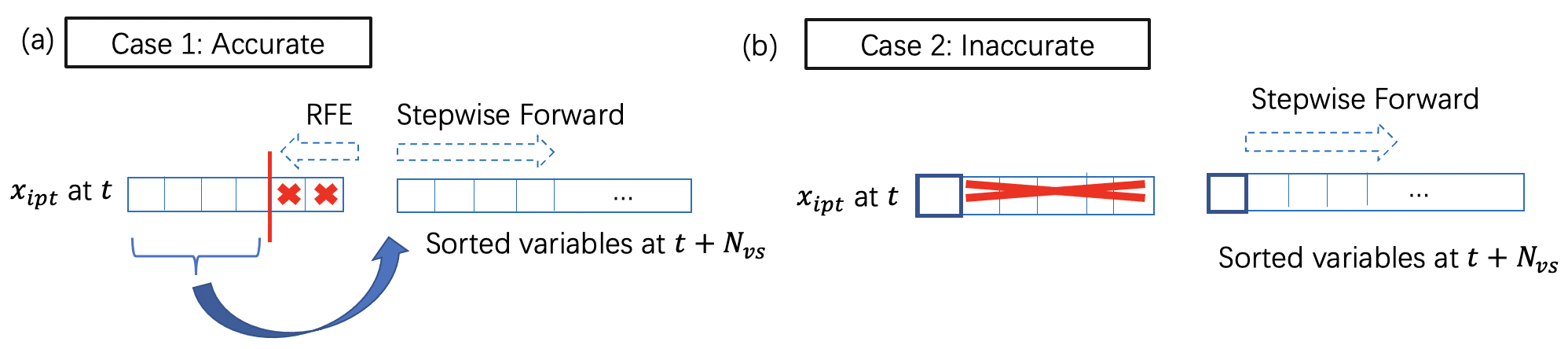
Figure 1: Momentum mechanism in VS-BO. (a) Accurate case, RFE is first used to remove redundant variables, and then new variables are added. (b) Inaccurate case, most variables are removed except those that are considered very important in both variable selection steps (blue box). New variables are then added.

3.3 Sampling for unimportant variables

We propose a method based on Covariance Matrix Adaptation Evolution Strategy (CMA-ES) to obtain the new value of unimportant variables for each iteration. CMA-ES is an evolutionary algorithm for numerically optimizing a function. For each generation $k$, the algorithm samples new offsprings from a multivariate Gaussian distribution $\mathcal{N}\left(m^{(k-1)},(\sigma^{(k-1)})^{2}\right)$ and updates $m^{(k-1)}$ and $(\sigma^{(k-1)})^{2}$ based on these new samples and their corresponding function values. Details of this algorithm can be seen in Hansen (2016).

Using the same approach as CMA-ES, VS-BO uses the initialized data $\{(\mathbf{x}^{i},y^{i})\}_{i=1}^{N_{init}}$ to initialize the multivariate Gaussian distribution $p(\mathbf{x}\mid\mathcal{D})$ (line 5 in Algorithm 1), and for every $N_{vs}$ iterations, it updates the distribution based on new query-output pairs (line 9 in Algorithm 1). Because of the property of Gaussian distribution, the conditional distribution $p(\mathbf{x}_{nipt}\mid\mathbf{x}_{ipt},\mathcal{D})$ is easily derived which is also a multivariate Gaussian distribution. Therefore, $\mathbf{x}_{nipt}^{t}$ can be sampled from the Gaussian distribution $p(\mathbf{x}_{nipt}\mid\mathbf{x}_{ipt}^{t},\mathcal{D})$ (line 13 in Algorithm 1) when $\mathbf{x}_{ipt}^{t}$ is obtained.

Compared to BO, it is much faster to update the evolutionary algorithm and obtain new queries, although these queries are less precise than those from BO. VS-BO takes advantage of the strength of these two methods by using them on different variables. Important variables are crucial to the function value, therefore VS-BO uses the framework of BO on them to obtain precise queries. Unimportant variables do not effect the function value too much so there is no need to spend large time budget to search for extremely precise queries. Hence, they are determined by CMA-ES to reduce runtime. In addition, when the variable selection step is inaccurate, VS-BO degenerates to an algorithm that is similar to CMA-ES rather than random sampling, therefore this sampling strategy may help improve the robustness of the performance of the whole algorithm.

4 Computational complexity analysis

From the theoretical perspective, we prove that running BO by only using those important variables is able to decrease the runtime of both the step of fitting the GP and maximizing the acquisition function. Specifically, we have the following proposition:

Proposition 4.1.

Suppose the cardinality of $\mathbf{x}_{ipt}$ is $p$ and the Quasi-Newton method (QN) is used for both fitting the GP and maximizing the acquisition function. Under the choice of commonly used kernel functions and acquisition functions, if only variables in $\mathbf{x}_{ipt}$ is used, then the complexity of each step of QN is $\mathcal{O}(p^{2}+pn^{2}+n^{3})$ for fitting the GP and $\mathcal{O}(p^{2}+pn+n^{2})$ for maximizing the acquisition function, where $n$ is the number of queries that are already obtained.

The proof is in section B of the appendix. Note that the method for fitting the GP and maximizing the acquisition function under the framework of BoTorch is limited-memory BFGS, which is indeed a QN method. Since the complexity is related to the quadratic of $p$, selecting a small subset of variables (so that $p$ is small) can decrease the runtime of BO. Figure 6 empirically shows that compared to vanilla BO, VS-BO can both reduce the runtime of fitting a GP and optimizing the acquisition function, especially when $n$ is not small.

5 Regret bound analysis

Let $\mathbf{x}^{*}$ be one of the maximal points of $f(\mathbf{x})$. To quantify the efficacy of the optimization algorithm, we are interested in the cumulative regret $R_{N}$, defined as: $R_{N}=\sum_{t=1}^{N}\left[f(\mathbf{x}^{*})-f(\mathbf{x}^{t})\right]$ where $\mathbf{x}^{t}$ is the query at iteration $t$. Intuitively, the algorithm is better when $R_{N}$ is small, and a desirable property is to have no regret: $\lim_{N\to\infty}R_{N}/N=0$. Here, we provide an upper bound of the cumulative regret for a simplified VS-BO algorithm, called VS-GP-UCB (Algorithm 6 in the appendix). Similar to Srinivas et al. (2009), for proving the regret bound we need the smoothness assumption of the kernel function. In addition, we have the extra assumption that the $D-d$ variables in $\mathbf{x}$ are unimportant (for convenience we index unimportant variables from $d+1$ to $D$ without loss of generality), meaning the absolute values of partial derivatives of $f$ on those $D-d$ variables are in general smaller than those on important variables. Formally, we have the following assumption:

Assumption 5.1.

Let $\mathcal{X}\subset[0,1]^{D}$ be compact and convex, $D\in\mathbb{N}$, and $f$ be a sample path of a GP with mean zero and the kernel function $k$, which satisfies the following high probability bound on the derivatives of $f$ for some constants $a,b>0$, $1>\alpha\geq 0$:

$$P(\sup_{\mathbf{x}\in\mathcal{X}}\mathinner{\!\left\lvert\frac{\partial f}{\partial\mathbf{x}_{j}}\right\rvert}>L)\leq a\exp\left(-\left(\frac{L}{b}\right)^{2}\right),j=1,\dots,d$$

And:

$$P(\sup_{\mathbf{x}\in\mathcal{X}}\mathinner{\!\left\lvert\frac{\partial f}{\partial\mathbf{x}_{j}}\right\rvert}>L)\leq a\exp\left(-\left(\frac{L}{\alpha b}\right)^{2}\right),j=d+1,\dots,D,$$

In VS-GP-UCB, the values of unimportant variables are fixed in advance (line 4 in Algorithm 6), denoted as $\mathbf{x}^{0}_{[d+1\mathrel{\mathop{\mathchar 58\relax}}D]}$, and the important variables are queried at each iteration by maximizing the acquisition function upper confidence bound (UCB) (Auer, 2002) with those fixed unimportant variables (line 6 in Algorithm 6). We have the following regret bound theorem of VS-GP-UCB:

Theorem 5.1.

Let $\mathcal{X}\subset[0,1]^{D}$ be compact and convex, suppose Assumption 5.1 is satisfied, pick $\delta\in(0,1)$, and define

$$\beta_{t}=2\log\frac{8\pi^{2}t^{2}}{3\delta}+2(D-d)\log\left(\alpha Dt^{2}b\sqrt{\log\left(\frac{8Da}{\delta}\right)}+1\right)+2d\log\left(Dt^{2}b\sqrt{\log\left(\frac{8Da}{\delta}\right)}\right).$$

Running the VS-GP-UCB, with probability $\geq 1-\delta$, we have:

$$\frac{R_{N}}{N}=\frac{\sum_{t=1}^{N}r_{t}}{N}\leq 2\sqrt{C_{1}\frac{\beta_{N}\gamma_{N}}{N}}+\frac{\pi^{2}}{3N}+\alpha b\sqrt{\log\left(\frac{8Da}{\delta}\right)}(D-d),$$

Here, $\gamma_{N}\mathrel{\mathop{\mathchar 58\relax}}=\max_{A\subset\mathcal{X}\mathrel{\mathop{\mathchar 58\relax}}|A|=N}\mathbf{I}(\mathbf{y}_{A};\mathbf{f}_{A})$ is the maximum information gain with a finite set of sampling points $A$, $\mathbf{f}_{A}=[f(\mathbf{x})]_{\mathbf{x}\in A}$, $\mathbf{y}_{A}=\mathbf{f}_{A}+\epsilon_{A}$, and $C_{1}=\frac{8}{\log\left(1+\sigma_{0}^{-2}\right)}$.

The proof of Theorem 5.1 is in section C of the appendix. Srinivas et al. (2009) upper bounded the maximum information gain for some commonly used kernel functions, for example they prove that by using SE kernel with the same length scales ($\rho_{i}=\rho_{0}$ for all $i$), $\gamma_{N}=\mathcal{O}\left((\log N)^{D+1}\right)$ so that $\lim_{N\to\infty}(\beta_{N}\gamma_{N})/N=0$. However, every variable is equally important in the SE kernel with the same length scales, which does not obey Assumption 5.1. We hypothesize that by using SE kernel of which the length scales are different such that Assumption 5.1 is satisfied, the statement that $\lim_{N\to\infty}(\beta_{N}\gamma_{N})/N=0$ is also correct, although we do not have proof here.

Li et al. (2016) also derives a regret bound for its dropout algorithm (Lemma 5 in Li et al. (2016)). Compared to the regret bound in Srinivas et al. (2009) (Theorem 2 in Srinivas et al. (2009)), both Li et al. (2016) and our work have an additional residual in the bound, while ours contains a small coefficient $\alpha$. In the case when $\alpha\to 0$, the bound in Theorem 5.1 is the same as that in theorem 2 of Srinivas et al. (2009) and there is no regret. These results show the necessity of the variable selection since it can help decrease the value of $\alpha$. In addition, compared to fixing unimportant variables in VS-GP-UCB, sampling from the CMA-ES posterior may further decrease the residual value.

6 Experiments

We compare VS-BO to a broad selection of existing methods: vanilla BO, REMBO and its variant REMBO Interleave, Dragonfly, HeSBO and ALEBO. The details of implementations of these methods as well as hyperparameter settings are described in section D of the appendix.

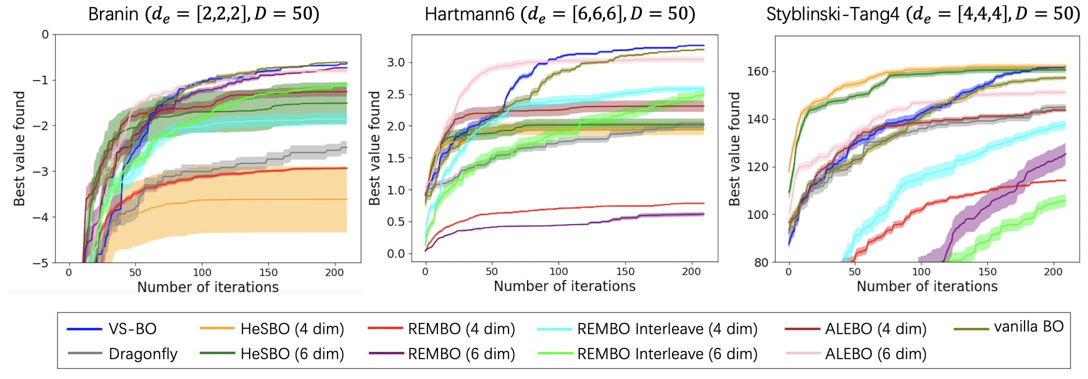
Figure 2: Performance of BO methods on Branin, Hartmann6 and Styblinski-Tang4 test functions. For each test function, we do 20 independent runs for each method. We plot the mean and 1/8 standard deviation of the best maximum value found by iterations.

6.1 Synthetic problems

We use the Branin ($d_{e}=2$), Hartmann6 ($d_{e}=6$) and Styblinski-Tang4 ($d_{e}=4$) functions as test functions. Previous high-dimensional BO work extends these functions to high dimension by adding unrelated variables, while in our work we present a harder test setting that has not been tried before by adding both unrelated and unimportant (but not totally unrelated) variables. For example, in the Hartmann6 case with the standard Hartmann6 function $f_{Hartmann6}(\mathbf{x}_{[1\mathrel{\mathop{\mathchar 58\relax}}6]})$ we first construct a new function $F_{hm6}(\mathbf{x})$ by adding variables with different importance, $F_{hm6}(\mathbf{x})=f_{Hartmann6}(\mathbf{x}_{[1\mathrel{\mathop{\mathchar 58\relax}}6]})+0.1f_{Hartmann6}(\mathbf{x}_{[7\mathrel{\mathop{\mathchar 58\relax}}12]})+0.01f_{Hartmann6}(\mathbf{x}_{[13\mathrel{\mathop{\mathchar 58\relax}}18]})$, and we further extend it to $D=50$ by adding unrelated variables; see section D for full details. The dimension of effective subspace of $F_{hm6}$ is $18$, while the dimension of important variables is only $6$. We hope that VS-BO can find those important variables successfully. For each embedding-based methods we evalualte both $d=4$ and $d=6$.

Figures 2 and  4 show performance of VS-BO as well as other BO methods on these three synthetic functions. When the iteration budget is fixed (Figure 2), the best value in average found by VS-BO after $200$ iterations is the largest or slightly smaller than the largest in all three cases. When the wall clock time or CPU time budget for BO is fixed (Figure 4), results show that VS-BO can find a large function value with high computational efficiency. Figure 5 shows that VS-BO can accurately find all the real important variables and meanwhile control false positives. We also test VS-BO on the function that has a non-axis-aligned subspace, and results in Figure 7 show that VS-BO also performs well. Vanilla BO under the framework of BoTorch can also achieve good performance for the fixed iteration budget, however, it is very computationally inefficient. For embedding-based methods, the results reflect some of their shortcomings. First, the performance of these methods are more variable than VS-BO; for example, HeSBO with $d=6$ performs very well in the Styblinski-Tang4 case but not in the others; Second, embedding-based methods are sensitive to the choice of the embedding dimension $d$, they perform especially bad when $d$ is smaller than the dimension of important variables (see results of the Hartmann6 case) and may still perform not well even when $d$ is larger (such as ALEBO with $d=6$ in the Styblinski-Tang4 case), while VS-BO can automatically learn the dimension. One advantage of embedding-based methods is that they may have a better performance than VS-BO within a very limited iteration budget (for example 50 iterations), which is expected since a number of data points are needed for VS-BO to make the variable selection accurate.

6.2 Real-world problems

We compare VS-BO with other methods on two real-world problems. First, VS-BO is tested on the rover trajectory optimization problem presented in Wang et al. (2017), a problem with a $60$-dimensional input domain. Second, it is tested on the vehicle design problem MOPTA08 (Jones, 2008), a problem with $124$ dimensions. On these two problems, we evaluate both $d=6$ and $d=10$ for each embedding-based method, except we omit ALEBO with $d=10$ since it is very time consuming. The detailed settings of these two problems are described in section D of the appendix.

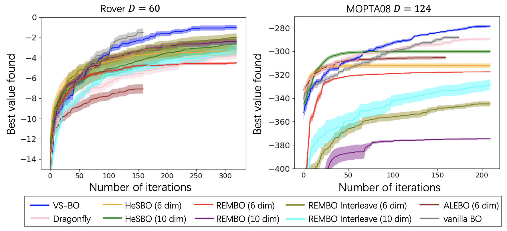
Figure 3: Performance of BO methods on the rover trajectory and MOPTA08 problems. We do 20 independent runs on the rover trajectory problem and 15 on the MOPTA08 problem. We plot the mean and 1/4 standard deviation of the best maximum value found by iterations. Curves of vanilla BO and ALEBO with $d=6$ do not reach the maximum iteration since they are time consuming and cannot run the maximum within the wall clock time budget (3600 seconds for the rover trajectory problem for each run and 4800 seconds for the MOPTA08 problem).

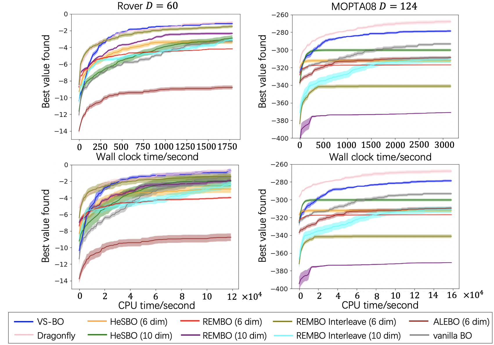
Figure 8: Performance of BO methods on the rover trajectory and MOPTA08 problems. We do 20 independent runs on the rover trajectory problem and 15 on the MOPTA08 problem. We plot the mean and 1/4 standard deviation of the best maximum value found by wall clock time (first row) and CPU time (second row).

Figures 3 and  8 show the performance of VS-BO and other BO methods on these two problems. When the iteration budget is fixed (Figure 3), VS-BO and vanilla BO have a better performance than other methods on both problems. When the wall clock or CPU time is fixed (Figure 8), Dragonfly and VS-BO reach the best performance on the rover trajectory problem, and Dragonfly performs the best on MOPTA08 problem while VS-BO has the second best performance. Vanilla BO is computationally inefficient so it does not have good performance with the fixed runtime. The left column of Figure 9 shows the frequency of being chosen as important for each variable when VS-BO is used. Since there is no ground truth of important variables in real-world cases, we use a sampling experiment to test whether those more frequently-chosen variables are more important. Specifically, we sample the first $5$ variables that have been chosen most frequently by a Sobol sequence and fix the values of other variables with the values in the best query we have found (the query having the highest function value). We then calculate the function values of this set of samples. Likewise, we also sample the first $5$ variables that have been chosen least frequently and evaluate the functions. The right column of Figure 9 shows that the variance of function values from the first set of samples is significantly higher than that from the second, especially on the MOPTA08 problem, indicating that those frequently selected variables indeed have more significant effect on the function value.

7 Conclusion

We propose a new method, VS-BO, for high-dimensional BO that is based on the assumption that variables of the input can be divided to two categories: important and unimportant. Our method can assign variables into these two categories with no need for pre-specifying any crucial hyper-parameter and use different strategies to decide values of the variables in different categories to reduce runtime. The good performance of our method on synthetic and real-world problems further verify the rationality of the assumption. We show the computational efficiency of our method both theoretically and empirically. In addition, information from the variable selection improves the interpretability of BO model: VS-BO can find important variables so that it can help increase our understanding of the black-box function. We also notice that in practice vanilla BO under the framework of BoTorch usually has a good performance if the runtime of BO does not need to be considered, especially when the dimension is not too large ($D<100$). However, this method is usually not considered as a baseline to compare with in previous high-dimensional BO work.

We also find some limitations of our method when running experiments. First, when the dimension of the input increases, it becomes harder to do variable selection accurately. Therefore, embedding-based methods are still the first choice when the input of a function has thousands of dimensions. It might be interesting to develop new algorithms that can do variable selection robustly even when the dimension is extremely large. Further, Grad-IS might be invalid when variables are discrete or categorical, therefore new methods for calculating the importance score of these kinds of variables are needed. These are several directions for future improvements of VS-BO. It is also interesting to do further theoretical study such as investigating the bounds on the maximum information gain of kernels that satisfy Assumption 5.1.

Checklist

1. For all authors…

   1. Do the main claims made in the abstract and introduction accurately reflect the paper’s contributions and scope? [Yes] The last paragraph of the introduction section describes the paper’s contributions.

   2. Did you describe the limitations of your work? [Yes] The last paragraph of the conclusion section describes some limitations of our work.

   3. Did you discuss any potential negative societal impacts of your work? [N/A] There will be no potential negative societal impacts of our work.

   4. Have you read the ethics review guidelines and ensured that your paper conforms to them? [Yes] I read it carefully.

2. If you are including theoretical results…

   1. Did you state the full set of assumptions of all theoretical results? [Yes] It is in section 5.

   2. Did you include complete proofs of all theoretical results? [Yes] It is in section B and C.

3. If you ran experiments…

   1. Did you include the code, data, and instructions needed to reproduce the main experimental results (either in the supplemental material or as a URL)? [Yes] Codes will be attached in the supplementary material.

   2. Did you specify all the training details (e.g., data splits, hyperparameters, how they were chosen)? [Yes] They are described in section D.

   3. Did you report error bars (e.g., with respect to the random seed after running experiments multiple times)? [Yes] For each case we repeat $20$ independent runs, and we plot mean and standard deviation in our figures.

   4. Did you include the total amount of compute and the type of resources used (e.g., type of GPUs, internal cluster, or cloud provider)? [Yes] They are described in section D.

4. If you are using existing assets (e.g., code, data, models) or curating/releasing new assets…

   1. If your work uses existing assets, did you cite the creators? [Yes]

   2. Did you mention the license of the assets? [N/A]

   3. Did you include any new assets either in the supplemental material or as a URL? [Yes] They are described in section D.

   4. Did you discuss whether and how consent was obtained from people whose data you’re using/curating? [N/A]

   5. Did you discuss whether the data you are using/curating contains personally identifiable information or offensive content? [N/A]

5. If you used crowdsourcing or conducted research with human subjects…

   1. Did you include the full text of instructions given to participants and screenshots, if applicable? [N/A]

   2. Did you describe any potential participant risks, with links to Institutional Review Board (IRB) approvals, if applicable? [N/A]

   3. Did you include the estimated hourly wage paid to participants and the total amount spent on participant compensation? [N/A]

Appendix A Variable selection with momentum mechanism

In this section, we provide pseudo-code for the algorithm of variable selection with momentum mechanism. Note that Algorithm 4 (momentum in the inaccurate case) is similar to Algorithm 2, except the lines that are marked with red color.

Algorithm 3 Variable Selection (VS) with Momentum

1:Input: iteration index $t$, $\mathcal{D}=\{(\mathbf{x}^{i},y^{i})\}_{i=1}^{t}$, $N_{init}$, $N_{vs}$, set of important variables chosen at iteration $t-N_{vs}$, denote as $\hat{\mathbf{x}}_{ipt}$

2:Output: Set of important variables chosen at iteration $t$, denote as $\mathbf{x}_{ipt}$

3:if $t=N_{init}+N_{vs}$ or $\hat{\mathbf{x}}_{ipt}=\mathbf{x}$ then $\triangleright$ First time to do variable selection or $\hat{\mathbf{x}}_{ipt}$ contains all variables

4:     return Algorithm 2

5:else if $\max_{k\in\{t-N_{vs}+1,t-N_{vs}+2,\dots,t\}}y^{k}\leq\max_{k\in\{1,\dots,t-N_{vs}\}}y^{k}$ then $\triangleright$ Inaccurate case

6:     return Algorithm 4

7:else$\triangleright$ Accurate case

8:     return Algorithm 5

9:end if

Algorithm 4 Momentum in the inaccurate case

1:Input: $\mathcal{D}=\{(\mathbf{x}^{i},y^{i})\}_{i=1}^{t}$, $N_{vs}$, set of important variables chosen at iteration $t-N_{vs}$, denote as $\hat{\mathbf{x}}_{ipt}$

2:Output: Set of important variables chosen at iteration $t$, denote as $\mathbf{x}_{ipt}$

3:Fit a GP to $\mathcal{D}$ and calculate important scores of variables $IS$ where $IS[i]$ is the important score of the i-th variable

4:Sort variables according to their important scores, $[\mathbf{x}_{s(1)},\dots,\mathbf{x}_{s(D)}]$, from the most important to the least

5:for $n=1,\ldots D$ do

6:     if $\mathbf{x}_{s(n)}\notin\hat{\mathbf{x}}_{ipt}$ then

7:         break

8:     end if

9:end for

10:for $m=n,n+1,\ldots D$ do $\triangleright$ Stepwise forward selection

11:     Fit a GP to $\mathcal{D}_{m}\mathrel{\mathop{\mathchar 58\relax}}=\{(\mathbf{x}_{s(1)\mathrel{\mathop{\mathchar 58\relax}}s(m)}^{i},y^{i})\}_{i=1}^{t-1}$ where $\mathbf{x}_{s(1)\mathrel{\mathop{\mathchar 58\relax}}s(m)}^{i}$ is the $i$-th input with only the first $m$ important variables, let $L_{m}$ to be the value of final negative marginal log likelihood

12:     if $m-n<2$ then

13:         continue

14:     else if $L_{m-1}-L_{m}\leq 0$ or $L_{m-1}-L_{m}<\frac{L_{m-2}-L(m-1)}{10}$ then

15:         break

16:     end if

17:end for

18:return $\mathbf{x}_{ipt}=\{\mathbf{x}_{s(1)},\dots,\mathbf{x}_{s(m-1)}\}$

Algorithm 5 Momentum in accurate case

1:Input: $\mathcal{D}=\{(\mathbf{x}^{i},y^{i})\}_{i=1}^{t}$, $N_{vs}$, set of important variables chosen at iteration $t-N_{vs}$, denoted as $\hat{\mathbf{x}}_{ipt}$, with cardinality $w=\mathinner{\!\left\lvert\hat{\mathbf{x}}_{ipt}\right\rvert}$

2:Output: Set of important variables chosen at iteration $t$, denote as $\mathbf{x}_{ipt}$

3:Fit a GP to $\mathcal{D}$ and calculate important scores of variables $IS$ where $IS[i]$ is the important score of the i-th variable

4:Sort variables according to $IS$, $[\mathbf{x}_{s(1)},\dots,\mathbf{x}_{s(D)}]$, from the most important to the least

5:Fit a GP by using variables in $\hat{\mathbf{x}}_{ipt}$, i.e. fit a GP to $\{(\hat{\mathbf{x}}_{ipt}^{i},y^{i})\}_{i=1}^{t}$, and calculate important scores of these variables $\widehat{IS}$. Let $\hat{L}_{w}$ be the value of final negative marginal log likelihood

6:Sort variables in $\hat{\mathbf{x}}_{ipt}$ according to $\widehat{IS}$, $[\mathbf{x}_{s^{\prime}(1)},\dots,\mathbf{x}_{s^{\prime}(w)}]$, from the most important to the least.

7:for $m=w-1,w-2,\ldots 0$ do $\triangleright$ Recursive feature elimination

8:     if $m=0$ then

9:         Set $\mathbf{x}_{ipt}=\{\mathbf{x}_{s^{\prime}(1)}\}$

10:         break

11:     end if

12:     Fit a GP by only using the first $m$ important variables according to $\widehat{IS}$. Let $\hat{L}_{m}$ to be the value of final negative marginal log likelihood

13:     if $\hat{L}_{m}>\hat{L}_{m+1}$ then

14:         Set $\mathbf{x}_{ipt}=\{\mathbf{x}_{s^{\prime}(1)},\dots,\mathbf{x}_{s^{\prime}(m+1)}\}$

15:         Set $L_{0}=\hat{L}_{m+1}$

16:         break

17:     end if

18:end for

19:for $m=1,2,\ldots D$ do $\triangleright$ Stepwise forward selection

20:     if $\mathbf{x}_{s(m)}\in\mathbf{x}_{ipt}$ then

21:         Set $L_{m}=L_{m-1}$, $L_{m-1}=L_{m-2}$

22:         continue

23:     end if

24:     Fit a GP by using variables in $\mathbf{x}_{ipt}\cup\{\mathbf{x}_{s(m)}\}$. Let $L_{m}$ to be the value of final negative marginal log likelihood

25:     if $m<2$ then

26:         $\mathbf{x}_{ipt}=\mathbf{x}_{ipt}\cup\{\mathbf{x}_{s(m)}\}$

27:         continue

28:     else if $L_{m-1}-L_{m}\leq 0$ or $L_{m-1}-L_{m}<\frac{L_{m-2}-L(m-1)}{10}$ then

29:         break

30:     end if

31:     $\mathbf{x}_{ipt}=\mathbf{x}_{ipt}\cup\{\mathbf{x}_{s(m)}\}$

32:end for

33:return $\mathbf{x}_{ipt}$

Appendix B Proof of Proposition 4.1

Proof of Proposition 4.1.

Given query-output pairs $\mathcal{D}=\{(\mathbf{x}^{i},y^{i})\}_{i=1}^{n}$, the marginal log likelihood (MLL) that need to be maximized at the step of fitting a GP has the following explicit form:

$$\log p(\Theta=\{\rho^{2}_{1\mathrel{\mathop{\mathchar 58\relax}}D},\alpha_{0}^{2}\},\sigma_{0}\mid\mathcal{D})=-\frac{1}{2}\mathbf{y}M^{-1}\mathbf{y}^{\top}-\frac{1}{2}\log\mathinner{\!\left\lvert M\right\rvert}-\frac{n\log 2\pi}{2}$$

where $\mathbf{y}=[y^{1},\ldots y^{n}]$ is an $n$-dimensional vector and $M=\left(K(\mathbf{x}^{1\mathrel{\mathop{\mathchar 58\relax}}n},\Theta)+\sigma^{2}_{0}\mathbf{I}\right)$. When the quasi-Newton method is used for maximizing MLL, the gradient should be calculated for each iteration:

$$\bigtriangledown_{\Theta,\sigma_{0}}\log p(\Theta,\sigma_{0}\mid\mathcal{D})=-\frac{1}{2}\mathbf{y}M^{-1}\left(\bigtriangledown_{\Theta,\sigma_{0}}M\right)M^{-1}\mathbf{y}^{\top}-\frac{1}{2}\textbf{tr}\left(M^{-1}\left(\bigtriangledown_{\Theta,\sigma_{0}}M\right)\right)$$

When only variables in $\mathbf{x}_{ipt}$ are used, we define the distance between two queries $\mathbf{x}^{i}$ and $\mathbf{x}^{j}$ as:

$$d(\mathbf{x}^{i},\mathbf{x}^{j})=\sqrt{\sum_{m\mathrel{\mathop{\mathchar 58\relax}}m\in\mathbf{x}_{ipt}}\rho_{m}^{2}(\mathbf{x}_{m}^{i}-\mathbf{x}_{m}^{j})^{2}}$$

and all the other inverse squared length scales corresponding to unimportant variables are fixed to $0$. Commonly chosen kernel functions are actually functions of the distance defined above, for example the squared exponential (SE) kernel is as the following:

$$k_{SE}(\mathbf{x}^{i},\mathbf{x}^{j},\Theta)=\alpha_{0}^{2}\exp\left(-\frac{1}{2}d^{2}(\mathbf{x}^{i},\mathbf{x}^{j})\right)$$

and the Matern-5/2 kernel is as the following:

$$k_{Mt}(\mathbf{x}^{i},\mathbf{x}^{j},\Theta)=\alpha_{0}^{2}\left(1+\sqrt{5}d(\mathbf{x}^{i},\mathbf{x}^{j})+\frac{5}{3}d^{2}(\mathbf{x}^{i},\mathbf{x}^{j})\right)\exp\left(-\sqrt{5}d(\mathbf{x}^{i},\mathbf{x}^{j})\right)$$

Since the cardinality of $\mathbf{x}_{ipt}$ is $p$, the cardinality of parameters in the kernel function that are not fixed to $0$ is $p+1$, hence the complexity of calculating the gradient of the distance is $\mathcal{O}(p)$, therefore whatever using SE kernel or Matern-5/2 kernel, the complexity of calculating $\bigtriangledown_{\Theta}k(\mathbf{x}^{i},\mathbf{x}^{j},\Theta)$ is $\mathcal{O}(p)$.

Since $M$ is a $n\times n$ matrix and each entry $M_{ij}$ equals to $k(\mathbf{x}^{i},\mathbf{x}^{j},\Theta)+\sigma_{0}^{2}\mathbbm{1}(i=j)$, the complexity of calculating $\bigtriangledown_{\Theta,\sigma_{0}}M$ is $\mathcal{O}(pn^{2})$. the complexity of calculating the inverse matrix $M^{-1}$ is $\mathcal{O}(n^{3})$ in general, and the following matrix multiplication and trace calculation need $\mathcal{O}(pn^{2})$, therefore the complexity of calculating the gradient of MLL is $\mathcal{O}(pn^{2}+n^{3})$. Once the gradient is obtained, each quasi-Newton step needs additional $\mathcal{O}(p^{2})$, therefore the complexity of one step of quasi-Newton method when fitting a GP is $\mathcal{O}(p^{2}+pn^{2}+n^{3})$.

As described in section 2, the acquisition function is a function that depends on the posterior mean $\mu$ and the posterior standard deviation $\sigma$, hence the gradients of $\mu$ and $\sigma$ should be calculated when the gradient of the acquisition function is needed.

When only variables in $\mathbf{x}_{ipt}$ are used, the gradient of $\mu$ with respect to $\mathbf{x}_{ipt}$ has the following form:

$$\bigtriangledown_{\mathbf{x}_{ipt}}\mu(\mathbf{x}_{ipt}\mid\mathcal{D})=\left(\bigtriangledown_{\mathbf{x}_{ipt}}K(\mathbf{x}_{ipt},\mathbf{x}^{1\mathrel{\mathop{\mathchar 58\relax}}n}_{ipt})\right)\left(K(\mathbf{x}^{1\mathrel{\mathop{\mathchar 58\relax}}n}_{ipt},\Theta)+\sigma^{2}_{0}\mathbf{I}\right)^{-1}\mathbf{y}^{\top}$$

Here $\left(K(\mathbf{x}^{1\mathrel{\mathop{\mathchar 58\relax}}n}_{ipt},\Theta)+\sigma^{2}_{0}\mathbf{I}\right)^{-1}\mathbf{y}^{\top}$ is fixed so that its value can be calculated in advance and stored as a $n$-dimensional vector. $K(\mathbf{x}_{ipt},\mathbf{x}^{1\mathrel{\mathop{\mathchar 58\relax}}n}_{ipt})$ is a $n$-dimensional vector of which each element is a kernel value between $\mathbf{x}_{ipt}$ and $\mathbf{x}_{ipt}^{i}$, hence the complexity of calculating the gradient of each element in $K(\mathbf{x}_{ipt},\mathbf{x}^{1\mathrel{\mathop{\mathchar 58\relax}}n}_{ipt})$ is $\mathcal{O}(p)$. Therefore, the complexity is $\mathcal{O}(pn)$ to calculate $\bigtriangledown_{\mathbf{x}_{ipt}}K(\mathbf{x}_{ipt},\mathbf{x}^{1\mathrel{\mathop{\mathchar 58\relax}}n}_{ipt})$ and $\mathcal{O}(pn)$ for additional matrix manipulation, hence the total complexity for calculating $\bigtriangledown_{\mathbf{x}_{ipt}}\mu(\mathbf{x}_{ipt}\mid\mathcal{D})$ is $\mathcal{O}(pn)$.

The gradient of $\sigma$ has the following form:

$$\bigtriangledown_{\mathbf{x}_{ipt}}\sigma(\mathbf{x}_{ipt}\mid\mathcal{D}) =\bigtriangledown_{\mathbf{x}_{ipt}}\sqrt{k(\mathbf{x}_{ipt},\mathbf{x}_{ipt},\Theta)-K(\mathbf{x}_{ipt},\mathbf{x}_{ipt}^{1\mathrel{\mathop{\mathchar 58\relax}}n})[K(\mathbf{x}_{ipt}^{1\mathrel{\mathop{\mathchar 58\relax}}n},\Theta)+\sigma^{2}_{0}\mathbf{I}]^{-1}K(\mathbf{x}_{ipt},\mathbf{x}_{ipt}^{1\mathrel{\mathop{\mathchar 58\relax}}n})^{\top}}$$

$$=-\frac{\left(\bigtriangledown_{\mathbf{x}_{ipt}}K(\mathbf{x}_{ipt},\mathbf{x}^{1\mathrel{\mathop{\mathchar 58\relax}}n}_{ipt})\right)\left(K(\mathbf{x}^{1\mathrel{\mathop{\mathchar 58\relax}}n}_{ipt},\Theta)+\sigma^{2}_{0}\mathbf{I}\right)^{-1}}{\sqrt{k(\mathbf{x}_{ipt},\mathbf{x}_{ipt},\Theta)-K(\mathbf{x}_{ipt},\mathbf{x}_{ipt}^{1\mathrel{\mathop{\mathchar 58\relax}}n})[K(\mathbf{x}_{ipt}^{1\mathrel{\mathop{\mathchar 58\relax}}n},\Theta)+\sigma^{2}_{0}\mathbf{I}]^{-1}K(\mathbf{x}_{ipt},\mathbf{x}_{ipt}^{1\mathrel{\mathop{\mathchar 58\relax}}n})^{\top}}}$$

Once $\bigtriangledown_{\mathbf{x}_{ipt}}K(\mathbf{x}_{ipt},\mathbf{x}^{1\mathrel{\mathop{\mathchar 58\relax}}n}_{ipt})$ is calculated, $\mathcal{O}(pn+n^{2})$ is needed for additional matrix manipulation, hence the total complexity for calculating $\bigtriangledown_{\mathbf{x}_{ipt}}\sigma(\mathbf{x}_{ipt}\mid\mathcal{D})$ is $\mathcal{O}(pn+n^{2})$.

For commonly used acquisition functions such as upper confidence bound (UCB) [Auer, 2002]:

$$UCB(\mathbf{x}_{ipt}\mid\mathcal{D})=\mu(\mathbf{x}_{ipt}\mid\mathcal{D})+\sqrt{\beta_{n}}\sigma(\mathbf{x}_{ipt}\mid\mathcal{D})$$

and expected improvement (EI) [Močkus, 1975]:

$$EI(\mathbf{x}_{ipt}\mid\mathcal{D})=\left(\mu(\mathbf{x}_{ipt}\mid\mathcal{D})-y^{*}_{n}\right)\Phi\left(\frac{\mu(\mathbf{x}_{ipt}\mid\mathcal{D})-y^{*}_{n}}{\sigma(\mathbf{x}_{ipt}\mid\mathcal{D})}\right)+\sigma(\mathbf{x}_{ipt}\mid\mathcal{D})\varphi\left(\frac{\mu(\mathbf{x}_{ipt}\mid\mathcal{D})-y^{*}_{n}}{\sigma(\mathbf{x}_{ipt}\mid\mathcal{D})}\right)$$

where $y_{n}^{*}=\max_{i\leq n}y^{i}$, $\Phi(\cdot)$ is the cumulative distribution function of the standard normal distribution, and $\varphi(\cdot)$ is the probability density function, once the gradients of $\mu$ and $\sigma$ are derived, only additional $\mathcal{O}(p)$ is needed for vector calculation, hence the total complexity of calculating the gradient of the acquisition function is $\mathcal{O}(pn+n^{2})$. Again, once the gradient is obtained, each quasi-Newton step needs additional $\mathcal{O}(p^{2})$, therefore the complexity of one step of quasi-Newton method for maximising the acquisition function is $\mathcal{O}(p^{2}+pn+n^{2})$.

∎

Algorithm 6 VS-GP-UCB

1:Input: domain $\mathcal{X}$, GP prior with mean $\mu_{0}=0$ and the kernel function $k$, maximal iteration $N$

2:Output: Approximate maximizer $\mathbf{x}^{max}$

3:Let $\mathcal{D}=\emptyset$

4:Fix the last $D-d$ variables, $\mathbf{x}_{[d+1\mathrel{\mathop{\mathchar 58\relax}}D]}^{0}$

5:for $t=1,2,\ldots N$ do

6:     Choose $\mathbf{x}^{t}_{[1\mathrel{\mathop{\mathchar 58\relax}}d]}=\operatorname*{arg\,max}_{\mathbf{x}_{[1\mathrel{\mathop{\mathchar 58\relax}}d]}}\mu(\{\mathbf{x}_{[1\mathrel{\mathop{\mathchar 58\relax}}d]},\mathbf{x}^{0}_{[d+1\mathrel{\mathop{\mathchar 58\relax}}D]}\}\mid\mathcal{D})+\sqrt{\beta_{t}}\sigma(\{\mathbf{x}_{[1\mathrel{\mathop{\mathchar 58\relax}}d]},\mathbf{x}^{0}_{[d+1\mathrel{\mathop{\mathchar 58\relax}}D]}\}\mid\mathcal{D})$

7:     Sample $y^{t}=f\left(\mathbf{x}^{t}=\{\mathbf{x}_{[1\mathrel{\mathop{\mathchar 58\relax}}d]}^{t},\mathbf{x}_{[d+1\mathrel{\mathop{\mathchar 58\relax}}D]}^{0}\}\right)+\epsilon_{t}$, where $\epsilon_{t}\sim\mathcal{N}(0,\sigma_{0}^{2})$ is a noise

8:     Update $\mathcal{D}=\mathcal{D}\cup\{(\mathbf{x}^{t},y^{t})\}$

9:end for

10:return $\mathbf{x}^{max}$ that is equal to $\mathbf{x}^{i}$ with maximal $y^{i}$

Appendix C Proof of Theorem 5.1

We show the details of VS-GP-UCB and provide the proof of Theorem 5.1 below.

Proof of Theorem 5.1.

The second inequality of Assumption 5.1 is equivalent to the following inequality:

$$P(\sup_{\mathbf{x}\in\mathcal{X}}\mathinner{\!\left\lvert\frac{\partial f}{\partial\mathbf{x}_{j}}\right\rvert}>\alpha L)\leq a\exp\left(-\left(\frac{L}{b}\right)^{2}\right),j=d+1,\dots,D$$

Therefore, according to Assumption 5.1 and the union bound, we have that $w.p.\geq 1-Da\exp\left(-\left(\frac{L}{b}\right)^{2}\right)$:

$$\forall\mathbf{x},\mathbf{x}^{\prime}\in\mathcal{X},\mathinner{\!\left\lvert f(\mathbf{x})-f(\mathbf{x}^{\prime})\right\rvert}\leq L\mathinner{\!\left\lVert\mathbf{x}_{[1\mathrel{\mathop{\mathchar 58\relax}}d]}-\mathbf{x}^{\prime}_{[1\mathrel{\mathop{\mathchar 58\relax}}d]}\right\rVert}_{1}+\alpha L\mathinner{\!\left\lVert\mathbf{x}_{[d+1\mathrel{\mathop{\mathchar 58\relax}}D]}-\mathbf{x}^{\prime}_{[d+1\mathrel{\mathop{\mathchar 58\relax}}D]}\right\rVert}_{1}$$

Let $\frac{\delta}{2}=Da\exp\left(-\left(\frac{L}{b}\right)^{2}\right)$, meaning $L=b\sqrt{\log\left(\frac{2Da}{\delta}\right)}$, we have that $w.p.\geq 1-\frac{\delta}{2}$,

$$\forall\mathbf{x},\mathbf{x}^{\prime}\in\mathcal{X},\mathinner{\!\left\lvert f(\mathbf{x})-f(\mathbf{x}^{\prime})\right\rvert}\leq b\sqrt{\log\left(\frac{2Da}{\delta}\right)}\left(\mathinner{\!\left\lVert\mathbf{x}_{[1\mathrel{\mathop{\mathchar 58\relax}}d]}-\mathbf{x}^{\prime}_{[1\mathrel{\mathop{\mathchar 58\relax}}d]}\right\rVert}_{1}+\alpha\mathinner{\!\left\lVert\mathbf{x}_{[d+1\mathrel{\mathop{\mathchar 58\relax}}D]}-\mathbf{x}^{\prime}_{[d+1\mathrel{\mathop{\mathchar 58\relax}}D]}\right\rVert}_{1}\right)$$

Algorithm 7 GP-UCB (Algorithm 1 in Srinivas et al. [2009])

1:Input: domain $\mathcal{X}$, GP prior with mean $\mu_{0}=0$ and the kernel function $k$, maximal iteration $N$

2:Output: Approximate maximizer $\mathbf{x}^{max}$

3:Let $\hat{\mathcal{D}}=\emptyset$

4:for $t=1,2,\ldots N$ do

5:     Choose $\hat{\mathbf{x}}^{t}=\operatorname*{arg\,max}_{\mathbf{x}\in\mathcal{X}}\hat{\mu}(\mathbf{x}\mid\hat{\mathcal{D}}=\{(\hat{\mathbf{x}}^{i},\hat{y}^{i})\}_{i=1}^{t-1})+\sqrt{\beta_{t}}\hat{\sigma}(\mathbf{x}\mid\hat{\mathcal{D}}=\{(\hat{\mathbf{x}}^{i},\hat{y}^{i})\}_{i=1}^{t-1})$

6:     Sample $\hat{y}^{t}=f\left(\hat{\mathbf{x}}^{t}\right)+\hat{\epsilon}_{t}$, where $\hat{\epsilon}_{t}\sim\mathcal{N}(0,\sigma_{0}^{2})$ is a noise

7:     Update $\hat{\mathcal{D}}=\hat{\mathcal{D}}\cup\{(\hat{\mathbf{x}}^{t},\hat{y}^{t})\}$

8:end for

9:return $\hat{\mathbf{x}}^{max}$ that is equal to $\hat{\mathbf{x}}^{i}$ with maximal $\hat{y}^{i}$

Now we consider the standard GP-UCB algorithm (Algorithm 7). Given the same GP prior and the same kernel function, since VS-GP-UCB and GP-UCB are two different algorithms, for each iteration they obtain different queries and have different posterior mean and standard deviation. We use the hat symbol to represent elements from GP-UCB, and in the following proof we use $\mu_{t}(\cdot)$ ($\hat{\mu}_{t}(\cdot)$) to represent $\mu(\cdot\mid\mathcal{D}=\{(\mathbf{x}^{i},y^{i})\}_{i=1}^{t})$ ($\hat{\mu}(\cdot\mid\hat{\mathcal{D}}=\{(\hat{\mathbf{x}}^{i},\hat{y}^{i})\}_{i=1}^{t})$) and $\sigma_{t}(\cdot)$ ($\hat{\sigma}_{t}(\cdot)$) to represent $\sigma(\cdot\mid\mathcal{D}=\{(\mathbf{x}^{i},y^{i})\}_{i=1}^{t})$ ($\hat{\sigma}(\cdot\mid\hat{\mathcal{D}}=\{(\hat{\mathbf{x}}^{i},\hat{y}^{i})\}_{i=1}^{t})$) for convenience.

Srinivas et al. [2009] has the following lemma:

Lemma C.1 (Lemma 5.6 in Srinivas et al. [2009]).

Consider subsets $\mathcal{X}_{t}\subset\mathcal{X}$ with finite size, $|\mathcal{X}_{t}|<\infty$, pick $\delta\in(0,1)$ and set $\beta_{t}=2\log\left(\frac{\mathinner{\!\left\lvert\mathcal{X}_{t}\right\rvert}\pi_{t}}{\delta}\right)$, where $\sum_{t\geq 1}\pi_{t}^{-1}=1,\pi_{t}>0$. Running GP-UCB, we have that

$$\mathinner{\!\left\lvert f(\mathbf{x})-\hat{\mu}_{t-1}(\mathbf{x})\right\rvert}\leq\sqrt{\beta_{t}}\hat{\sigma}_{t-1}(\mathbf{x})\quad\forall\mathbf{x}\in\mathcal{X}_{t},\forall t\geq 1$$

holds with probability $\geq 1-\delta$.

By using the same proof procedure, we can easily obtain the following lemma:

Lemma C.2.

Consider subsets $\mathcal{X}_{t}\subset\mathcal{X}$ with finite size, $|\mathcal{X}_{t}|<\infty$, pick $\delta\in(0,1)$ and set $\beta_{t}=2\log\left(\frac{\mathinner{\!\left\lvert\mathcal{X}_{t}\right\rvert}\pi_{t}}{\delta}\right)$, where $\sum_{t\geq 1}\pi_{t}^{-1}=1,\pi_{t}>0$. Running VS-GP-UCB, we have

$$\mathinner{\!\left\lvert f(\mathbf{x})-\mu_{t-1}(\mathbf{x})\right\rvert}\leq\sqrt{\beta_{t}}\sigma_{t-1}(\mathbf{x})\quad\forall\mathbf{x}\in\mathcal{X}_{t},\forall t\geq 1$$

holds with probability $\geq 1-\delta$.

Now consider $\mathcal{X}_{t}$ to be the following discretization: for each dimension $j=1,\dots,d$, discretize it with $\tau_{t}$ uniformly spaced points, and for each dimension $j=d+1,\dots,D$, discretize it with $\alpha\tau_{t}$ uniformly spaced points plus the j-th element in $\mathbf{x}^{t}$, $\mathbf{x}^{t}_{j}=\mathbf{x}^{0}_{j}$ (note that $\mathbf{x}^{t}_{j}$ is fixed when $j\geq d+1$). Denote $\widetilde{(\mathbf{x})}_{t}$ be the closest point in $\mathcal{X}_{t}$ to $\mathbf{x}$ under $L_{1}$ norm (note that $\mathbf{x}^{t}$ is the $t$-th query of the VS-GP-UCB algorithm, while $\widetilde{(\mathbf{x}^{t})}_{t^{\prime}}$ is its closet point in $\mathcal{X}_{t^{\prime}}$), then because of the smoothness assumption, we have $w.p.\geq 1-\frac{\delta}{2}$:

$$\mathinner{\!\left\lvert f(\mathbf{x})-f\left(\widetilde{(\mathbf{x})}_{t}\right)\right\rvert}\leq b\sqrt{\log\left(\frac{2Da}{\delta}\right)}\frac{d}{\tau_{t}}+\alpha b\sqrt{\log\left(\frac{2Da}{\delta}\right)}\frac{D-d}{\alpha\tau_{t}} =b\sqrt{\log\left(\frac{2Da}{\delta}\right)}\frac{D}{\tau_{t}},$$

$$\forall\mathbf{x}\in\mathcal{X},\forall t\geq 1$$

By choosing $\tau_{t}=Dt^{2}b\sqrt{\log\left(\frac{2Da}{\delta}\right)}$, we have $w.p.\geq 1-\frac{\delta}{2}$:

$$\mathinner{\!\left\lvert f(\mathbf{x})-f(\widetilde{(\mathbf{x})}_{t})\right\rvert}\leq\frac{1}{t^{2}}\quad\forall\mathbf{x}\in\mathcal{X},\forall t\geq 1$$

Under this situation, we have:

$$\mathinner{\!\left\lvert\mathcal{X}_{t}\right\rvert}=(\alpha\tau_{t}+1)^{D-d}\tau_{t}^{d}=\left(\alpha Dt^{2}b\sqrt{\log\left(\frac{2Da}{\delta}\right)}+1\right)^{D-d}\left(Dt^{2}b\sqrt{\log\left(\frac{2Da}{\delta}\right)}\right)^{d}$$

Combine with Lemma C.2, by setting:

$$\beta_{t}=2\log\left(\frac{4\mathinner{\!\left\lvert\mathcal{X}_{t}\right\rvert}\pi_{t}}{\delta}\right)=2\log\frac{4\pi_{t}}{\delta} +2(D-d)\log\left(\alpha Dt^{2}b\sqrt{\log\left(\frac{2Da}{\delta}\right)}+1\right)$$

$$+2d\log\left(Dt^{2}b\sqrt{\log\left(\frac{2Da}{\delta}\right)}\right)$$

then w.p. $\geq 1-\delta$:

$$\mathinner{\!\left\lvert f(\mathbf{x})-\mu_{t-1}\left(\widetilde{(\mathbf{x})}_{t}\right)\right\rvert} \leq\mathinner{\!\left\lvert f(\mathbf{x})-f\left(\widetilde{(\mathbf{x})}_{t}\right)+f\left(\widetilde{(\mathbf{x})}_{t}\right)-\mu_{t-1}\left(\widetilde{(\mathbf{x})}_{t}\right)\right\rvert}$$

$$\leq\mathinner{\!\left\lvert f(\mathbf{x})-f\left(\widetilde{(\mathbf{x})}_{t}\right)\right\rvert}+\mathinner{\!\left\lvert f\left(\widetilde{(\mathbf{x})}_{t}\right)-\mu_{t-1}\left(\widetilde{(\mathbf{x})}_{t}\right)\right\rvert}$$

$$\leq\frac{1}{t^{2}}+\sqrt{\beta_{t}}\sigma_{t-1}\left(\widetilde{(\mathbf{x})}_{t}\right)\quad\forall\mathbf{x}\in\mathcal{X},\forall t\geq 1.$$

Likewise, by setting the same $\beta_{t}$, we have w.p. $\geq 1-\delta$:

$$\mathinner{\!\left\lvert f(\mathbf{x})-\hat{\mu}_{t-1}\left(\widetilde{(\mathbf{x})}_{t}\right)\right\rvert}\leq\frac{1}{t^{2}}+\sqrt{\beta_{t}}\hat{\sigma}_{t-1}\left(\widetilde{(\mathbf{x})}_{t}\right)\quad\forall\mathbf{x}\in\mathcal{X},\forall t\geq 1.$$

Let $\mathbf{x}^{t}_{mix}=\{\hat{\mathbf{x}}^{t}_{[1\mathrel{\mathop{\mathchar 58\relax}}d]},\mathbf{x}_{[d+1\mathrel{\mathop{\mathchar 58\relax}}D]}^{0}\}$ (first $d$ variables are equal to those in $\hat{\mathbf{x}}^{t}$, and the others are equal to $\mathbf{x}_{[d+1\mathrel{\mathop{\mathchar 58\relax}}D]}^{0}$), again because of the smoothness assumption, we have $w.p.\geq 1-\frac{\delta}{2}$:

$$\mathinner{\!\left\lvert f(\mathbf{x}^{t}_{mix})-f(\hat{\mathbf{x}}^{t})\right\rvert}\leq\alpha b\sqrt{\log\left(\frac{2Da}{\delta}\right)}\mathinner{\!\left\lVert\mathbf{x}^{0}_{[d+1\mathrel{\mathop{\mathchar 58\relax}}D]}-\hat{\mathbf{x}}^{t}_{[d+1\mathrel{\mathop{\mathchar 58\relax}}D]}\right\rVert}_{1}\leq\alpha b\sqrt{\log\left(\frac{2Da}{\delta}\right)}(D-d)$$

Note that the point in $\mathcal{X}_{t}$ that is closest to $\mathbf{x}^{t}_{mix}$ is $\widetilde{(\mathbf{x}^{t}_{mix})}_{t}=\left\{\widetilde{(\hat{\mathbf{x}}^{t}_{[1\mathrel{\mathop{\mathchar 58\relax}}d]})}_{t},\mathbf{x}_{[d+1\mathrel{\mathop{\mathchar 58\relax}}D]}^{0}\right\}$ because all elements in $\mathbf{x}_{[d+1\mathrel{\mathop{\mathchar 58\relax}}D]}^{0}$ are contained in the discretization. Since $\mathbf{x}_{[1\mathrel{\mathop{\mathchar 58\relax}}d]}^{t}$ is the maximizer of UCB with fixed $D-d$ variables, we have:

$$\mu_{t-1}\left(\widetilde{(\mathbf{x}^{t}_{mix})}_{t}\right)+\sqrt{\beta_{t}}\sigma_{t-1}\left(\widetilde{(\mathbf{x}^{t}_{mix})}_{t}\right)\leq\mu_{t-1}(\mathbf{x}^{t})+\sqrt{\beta_{t}}\sigma_{t-1}(\mathbf{x}^{t})$$

Similarly, considering GP-UCB algorithm, we have:

$$\hat{\mu}_{t-1}(\widetilde{(\mathbf{x}^{*})}_{t})+\sqrt{\beta_{t}}\hat{\sigma}_{t-1}(\widetilde{(\mathbf{x}^{*})}_{t})\leq\hat{\mu}_{t-1}(\hat{\mathbf{x}}^{t})+\sqrt{\beta_{t}}\hat{\sigma}_{t-1}(\hat{\mathbf{x}}^{t})$$

To finish the proof, we need to use another lemma in Srinivas et al. [2009]:

Lemma C.3 (Lemma 5.5 in Srinivas et al. [2009]).

Let $\{\hat{\mathbf{x}}^{t}\}$ be a sequence of points chosen by GP-UCB, pick $\delta\in(0,1)$ and set $\beta_{t}=2\log\left(\frac{\pi_{t}}{\delta}\right)$, where $\sum_{t\geq 1}\pi_{t}^{-1}=1,\pi_{t}>0$. Then,

$$\mathinner{\!\left\lvert f(\hat{\mathbf{x}}^{t})-\hat{\mu}_{t-1}(\hat{\mathbf{x}}^{t})\right\rvert}\leq\sqrt{\beta_{t}}\hat{\sigma}_{t-1}(\hat{\mathbf{x}}^{t}),\forall t\geq 1$$

holds with probability $\geq 1-\delta$.

By using the same proof procedure, we can easily obtain the following lemma:

Lemma C.4.

Let $\{\mathbf{x}^{t}\}$ be a sequence of points chosen by VS-GP-UCB, pick $\delta\in(0,1)$ and set $\beta_{t}=2\log\left(\frac{\pi_{t}}{\delta}\right)$, where $\sum_{t\geq 1}\pi_{t}^{-1}=1,\pi_{t}>0$. Then,

$$\mathinner{\!\left\lvert f(\mathbf{x}^{t})-\mu_{t-1}(\mathbf{x}^{t})\right\rvert}\leq\sqrt{\beta_{t}}\sigma_{t-1}(\mathbf{x}^{t}),\forall t\geq 1$$

holds with probability $\geq 1-\delta$.

Finally, by using $\frac{\delta}{4}$ and setting (often set $\pi_{t}=\frac{\pi^{2}t^{2}}{6}$):

$$\beta_{t}=2\log\frac{16\pi_{t}}{\delta}+2(D-d)\log\left(\alpha Dt^{2}b\sqrt{\log\left(\frac{8Da}{\delta}\right)}+1\right)+2d\log\left(Dt^{2}b\sqrt{\log\left(\frac{8Da}{\delta}\right)}\right)$$

$w.p.\geq 1-\delta$ the simple regret $r_{t}$ of VS-GP-UCB, $r_{t}=f(\mathbf{x}^{*})-f(\mathbf{x}^{t}=\{\mathbf{x}_{[1\mathrel{\mathop{\mathchar 58\relax}}d]}^{t},\mathbf{x}_{[d+1\mathrel{\mathop{\mathchar 58\relax}}D]}^{0}\})$, is upper bounded by:

$$r_{t} =f(\mathbf{x}^{*})-f(\mathbf{x}^{t})$$

$$\leq\hat{\mu}_{t-1}(\widetilde{(\mathbf{x}^{*})}_{t})+\sqrt{\beta_{t}}\hat{\sigma}_{t-1}(\widetilde{(\mathbf{x}^{*})}_{t})+\frac{1}{t^{2}}-f(\mathbf{x}^{t})$$

$$\leq\hat{\mu}_{t-1}(\hat{\mathbf{x}}^{t})+\sqrt{\beta_{t}}\hat{\sigma}_{t-1}(\hat{\mathbf{x}}^{t})+\frac{1}{t^{2}}-f(\mathbf{x}^{t})$$

$$=\hat{\mu}_{t-1}(\hat{\mathbf{x}}^{t})+\sqrt{\beta_{t}}\hat{\sigma}_{t-1}(\hat{\mathbf{x}}^{t})-f(\hat{\mathbf{x}}^{t})+f(\hat{\mathbf{x}}^{t})-f(\mathbf{x}^{t}_{mix})+f(\mathbf{x}^{t}_{mix})-f(\mathbf{x}^{t})+\frac{1}{t^{2}}$$

$$\leq 2\sqrt{\beta_{t}}\hat{\sigma}_{t-1}(\hat{\mathbf{x}}^{t})+\alpha b\sqrt{\log\left(\frac{8Da}{\delta}\right)}(D-d)+\mu_{t-1}\left(\widetilde{(\mathbf{x}^{t}_{mix})}_{t}\right)$$

$$+\sqrt{\beta_{t}}\sigma_{t-1}\left(\widetilde{(\mathbf{x}^{t}_{mix})}_{t}\right)-f(\mathbf{x}^{t})+\frac{2}{t^{2}}$$

$$\leq 2\sqrt{\beta_{t}}\hat{\sigma}_{t-1}(\hat{\mathbf{x}}^{t})+\alpha b\sqrt{\log\left(\frac{8Da}{\delta}\right)}(D-d)+\mu_{t-1}(\mathbf{x}^{t})+\sqrt{\beta_{t}}\sigma_{t-1}(\mathbf{x}^{t})-f(\mathbf{x}^{t})+\frac{2}{t^{2}}$$

$$\leq 2\sqrt{\beta_{t}}\hat{\sigma}_{t-1}(\hat{\mathbf{x}}^{t})+2\sqrt{\beta_{t}}\sigma_{t-1}(\mathbf{x}^{t})+\frac{2}{t^{2}}+\alpha b\sqrt{\log\left(\frac{8Da}{\delta}\right)}(D-d)$$

By using Lemma 5.4 in Srinivas et al. [2009] and the Cauchy-Schwarz inequality, both $\sum_{t=1}^{N}2\sqrt{\beta_{t}}\hat{\sigma}_{t-1}(\hat{\mathbf{x}}^{t})$ and $\sum_{t=1}^{N}2\sqrt{\beta_{t}}\sigma_{t-1}(\mathbf{x}^{t})$ are upper bounded by $\sqrt{C_{1}N\beta_{N}\gamma_{N}}$, where $C_{1}=\frac{8}{\log\left(1+\sigma_{0}^{-2}\right)}$, and $\gamma_{N}\mathrel{\mathop{\mathchar 58\relax}}=\max_{A\subset\mathcal{X}\mathrel{\mathop{\mathchar 58\relax}}|A|=N}\mathbf{I}(\mathbf{y}_{A};\mathbf{f}_{A})$ is the maximum information gain with a finite set of sampling points $A$, $\mathbf{f}_{A}=[f(\mathbf{x})]_{\mathbf{x}\in A}$, $\mathbf{y}_{A}=\mathbf{f}_{A}+\epsilon_{A}$. Therefore, we have:

$$R_{N}=\sum_{t=1}^{N}r_{t}\leq 2\sqrt{C_{1}N\beta_{N}\gamma_{N}}+\frac{\pi^{2}}{3}+\alpha b\sqrt{\log\left(\frac{8Da}{\delta}\right)}N(D-d)$$

Hence:

$$\frac{R_{N}}{N}=\frac{\sum_{t=1}^{N}r_{t}}{N}\leq 2\sqrt{C_{1}\frac{\beta_{N}\gamma_{N}}{N}}+\frac{\pi^{2}}{3N}+\alpha b\sqrt{\log\left(\frac{8Da}{\delta}\right)}(D-d)$$

∎

Appendix D Detailed experimental settings and extended discussion of experimental results

We use the framework of BoTorch to implement VS-BO. We compare VS-BO to the following existing BO methods: vanilla BO, which is implemented by the standard BoTorch framework; REMBO and its variant REMBO Interleave [Wang et al., 2016], of which the implementations are based on Metzen [2016]; Dragonfly [Kandasamy et al., 2020], which contains the Add-GP method; HeSBO [Nayebi et al., 2019] which has already been implemented in Adaptive Experimentation Platform (Ax); And ALEBO [Letham et al., 2020]. By the time when we write this manuscript, source codes of the work Spagnol et al. [2019] and Eriksson and Jankowiak [2021] have not been released, so we cannot compare VS-BO with these two methods. Both VS-BO and vanilla BO use Matern 5/2 as the kernel function and expected improvement as the acquisition function, and use limited-memory BFGS (L-BFGS) to fit GP and optimize the acquisition function. The number of initialized samples $N_{init}$ is set to $5$ for all methods, and $N_{vs}$ in VS-BO is set to $20$, $N_{is}$ is set to $10000$ for all experiments. The number of the interleaved cycle for REMBO Interleave is set to $4$. Since our algorithm aims to maximize the black-box function, all the test functions that have minimum points will be converted to the corresponding negative forms.

In synthetic experiments, as described in section 6.1, for each test function we add some unimportant variables as well as unrelated variables to make it high-dimensional. The standard Branin function $f_{Branin}$ has two dimensions with the input domain $\mathcal{X}_{Branin}=[-5,10]\times[0,10]$, and we construct a new Branin function $F_{branin}$ as the following:

$$F_{branin}(\mathbf{x})=f_{Branin}(\mathbf{x}_{[1\mathrel{\mathop{\mathchar 58\relax}}2]})+0.1f_{Branin}(\mathbf{x}_{[3\mathrel{\mathop{\mathchar 58\relax}}4]}) +0.01f_{Branin}(\mathbf{x}_{[5\mathrel{\mathop{\mathchar 58\relax}}6]}),$$

$$\mathbf{x}\in\left(\bigotimes_{i=1}^{3}\mathcal{X}_{Branin}\right)\bigotimes_{i=1}^{44}[0,1]$$

where $\bigotimes$ represents the direct product. We use $d_{e}=[2,2,2]$ to represent the dimension of the effective subspace of $F_{branin}$, the total effective dimension is $6$, however, the number of important variables is only $2$.

Likewise, for the standard Hartmann6 function $f_{Hartmann6}$ that has six dimensions with the input domain $[0,1]^{6}$, we construct $F_{hm6}$ as:

$$F_{hm6}(\mathbf{x})=f_{Hartmann6}(\mathbf{x}_{[1\mathrel{\mathop{\mathchar 58\relax}}6]})+0.1f_{Hartmann6}(\mathbf{x}_{[7\mathrel{\mathop{\mathchar 58\relax}}12]})+0.01f_{Hartmann6}(\mathbf{x}_{[13\mathrel{\mathop{\mathchar 58\relax}}18]})\quad\mathbf{x}\in[0,1]^{50}$$

and use $d_{e}=[6,6,6]$ to represent the dimension of the effective subspace. For the Styblinski-Tang4 function $f_{ST4}$ that has four dimensions with the input domain $[-5,5]^{4}$, we construct $F_{ST4}$ as:

$$F_{ST4}(\mathbf{x})=f_{ST4}(\mathbf{x}_{[1\mathrel{\mathop{\mathchar 58\relax}}4]})+0.1f_{ST4}(\mathbf{x}_{[5\mathrel{\mathop{\mathchar 58\relax}}8]})+0.01f_{ST4}(\mathbf{x}_{[9\mathrel{\mathop{\mathchar 58\relax}}12]})\quad\mathbf{x}\in[-5,5]^{50}$$

and use $d_{e}=[4,4,4]$ to represent the dimension of the effective subspace. All synthetic experiments are run on the same Linux cluster that has 40 3.0 GHz 10-Core Intel Xeon E5-2690 v2 CPUs.

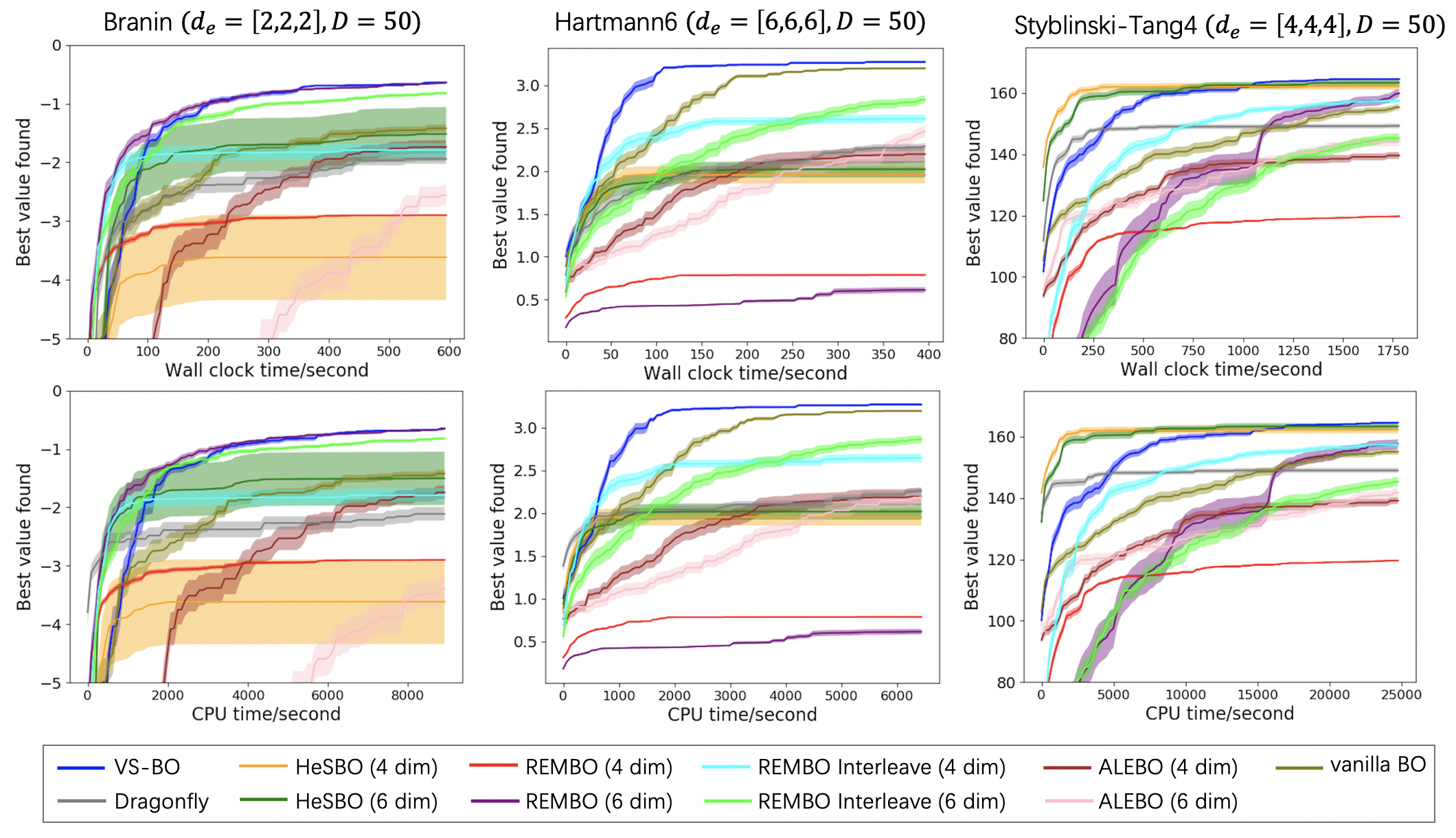
Figure 4: Performance of BO methods on Branin, Hartmann6 and Styblinski-Tang4 test functions. For each test function, we do 20 independent runs for each method. We plot the mean and 1/8 standard deviation of the best maximum value found by wall clock time used for BO (first row) and CPU time (second row).

Figure 2 and  4 show performances of different BO methods. They are compared under the fixed iteration budget (Figure 2), the fixed wall clock time budget used for BO itself (time for evaluating the black box function is excluded) or the fixed CPU time budget (Figure 4). Figure 5 shows the frequency of being chosen as important for each variable in steps of variable selection of VS-BO. Since we do 20 runs of VS-BO on each test function, each run has $210$ iterations and important variables are re-selected every $20$ iterations, the maximum frequency each variable can be chosen as important is $200$. In the Branin case with $d_{e}=[2,2,2]$, the first two variables are important, and the left panel of Figure 5 shows that the frequency of choosing the first two variables as important is significantly higher than that of choosing the other variables; In the Hartmann6 case with $d_{e}=[6,6,6]$, the first six variables are important, and the middle panel of Figure 5 shows that the frequency of choosing the first six variables as important is the highest; In the Styblinski-Tang4 case with $d_{e}=[4,4,4]$, the first four variables are important, and again the right panel of Figure 5 shows that the frequency of choosing the first four variables as important is the highest. These results indicate that VS-BO is able to find real important variables and control false positives.

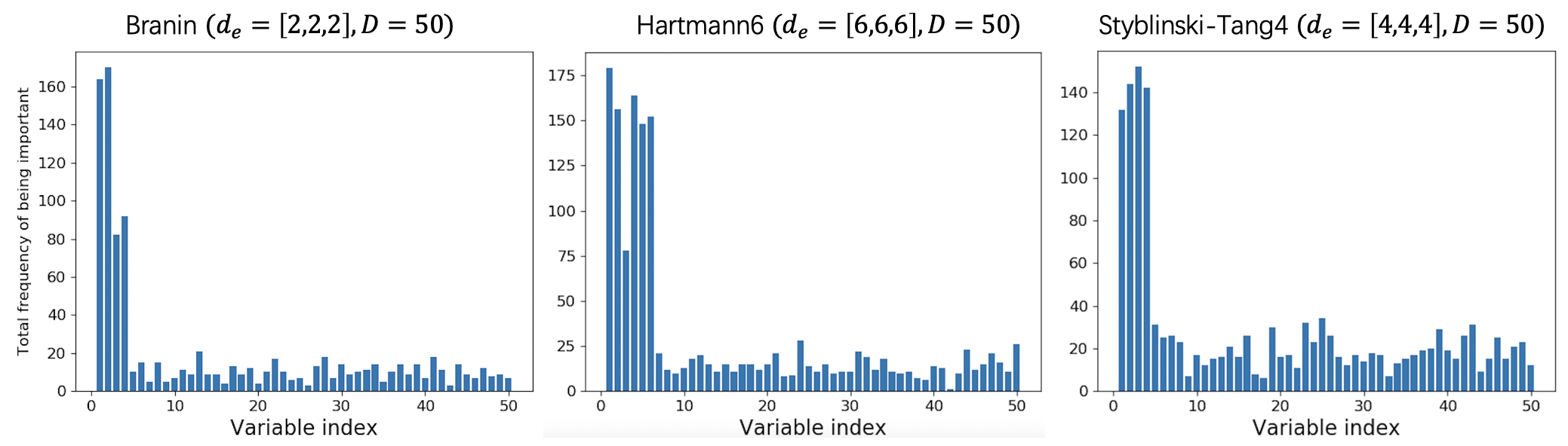
Figure 5: The total frequency of being chosen as important for each variable on Branin case (left), Hartmann6 case (middle) and Styblinski-Tang4 case (right). For the Branin function, the first two variables are important; for the Hartmann6 function, the first six variables are important; and for the Styblinski-Tang4 function, the first four variables are important.

Figure 6 shows the wall clock time or CPU time comparison between VS-BO and vanilla BO for each iteration under the step of fitting a GP or optimizing the acquisition function. As the number of iterations increases, the runtime of vanilla BO increases significantly, while for VS-BO the runtime only has a slight increase. These results empirically show that VS-BO is able to reduce the runtime of BO process.

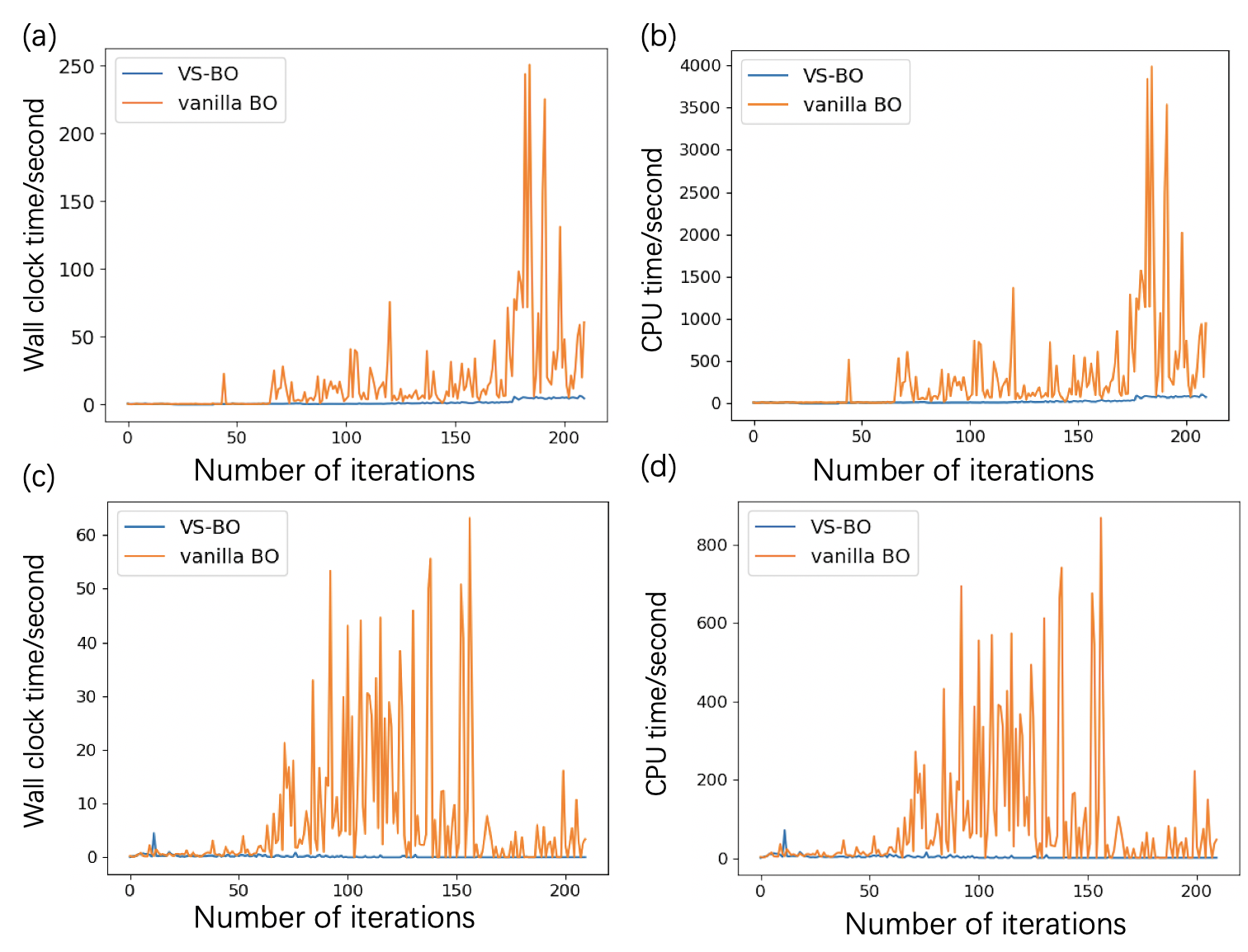
Figure 6: The wall clock time or CPU time comparison between VS-BO and vanilla BO for each iteration. The Branin test function with $d_{e}=[2,2,2]$ and $D=50$ is run here. (a) Wall clock time comparison at the GP fitting step (b) CPU time comparison at the GP fitting step (c) Wall clock time comparison at the acquisition function optimization step (d) CPU time comparison at the acquisition function optimization step

To test the performance of VS-BO on the function that has a non-axis-aligned subspace, we construct a rotational Hartmann6 function $F_{rot\_H}(\mathbf{x})$ by using the same way as Letham et al. [2020]. We sample a rotation matrix $A$ from the Haar distribution on the orthogonal group $SO(100)$ [Stewart, 1980], and take the form of $F_{rot\_H}(\mathbf{x})$ as the following:

$$F_{rot\_H}(\mathbf{x})=f_{Hartmann6}(A[\mathrel{\mathop{\mathchar 58\relax}}6]\mathbf{x})$$

where $A[\mathrel{\mathop{\mathchar 58\relax}}6]\in\mathbb{R}^{6\times 100}$ represents the first $6$ rows of $A$ and $\mathbf{x}\in[-1,1]^{100}$ is the input. We then run VS-BO as well as other methods on this function and compare their performance. Figure 7 shows that in this case REMBO with $d=6$ has the best performance. VS-BO also has a good performance, and surprisingly it outperforms several embedding-based methods such as ALEBO ($d=6$) and REMBO Interleave ($d=6$), although it tries to learn an axis-aligned subspace.

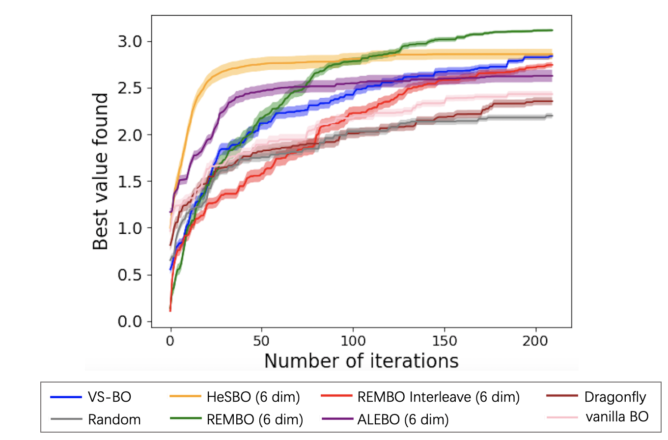
Figure 7: Performance of BO methods on the rotational Hartmann6 function. We do 20 independent runs for each method. We plot the mean and 1/8 standard deviation of the best maximum value found by iterations.

Spagnol et al. [2019] introduces several methods to sample unimportant variables and shows that the mix strategy is the best, that is for each iteration, the algorithm samples values of unimportant variables from the uniform distribution with probability $0.5$ or use the values from the previous query that has the maximal function value with probability $0.5$. To compare the mix strategy with our sampling strategy, i.e. sampling from CMA-ES related posterior, we replace our strategy with the mix strategy in VS-BO, creating a variant method called VSBO mix. All the other parts in VSBO mix are the same as those in VS-BO. We compare VS-BO with VSBO mix on these three synthetic functions, and Figure 10 show that in general our sampling strategy is clearly better than the mix strategy.

For real-world problems, the rover trajectory problem is a high-dimensional optimization problem with input domain $[0,1]^{60}$. The problem setting in our experiment is the same as that in Wang et al. [2017], and the source code of this problem can be found in https://github.com/zi-w/Ensemble-Bayesian-Optimization. MOPTA08 is another high-dimensional optimization problem with input domain $[0,1]^{124}$. It has one objective function $f_{mopta}(\mathbf{x})$ that needs to be minimized and $68$ constraints $c_{i}(\mathbf{x}),i\in\{1,2,\ldots 68\}$. Similar to Eriksson and Jankowiak [2021], we convert these constraints to soft penalties and convert the minimization problem to the maximization problem by adding a minus at the front of the objective function, i.e., we construct the following new function $F_{mopta}$:

$$F_{mopta}(\mathbf{x})=-\left(f_{mopta}(\mathbf{x})+10\sum_{i=1}^{68}\max(0,c_{i}(\mathbf{x}))\right)$$

The Fortran codes of MOPTA can be found in https://www.miguelanjos.com/jones-benchmark and we further use codes in https://gist.github.com/denis-bz/c951e3e59fb4d70fd1a52c41c3675187 to wrap up it in python. All experiments for these two real-world problems are run on the same Linux cluster that has 80 2.40 GHz 20-Core Intel Xeon 6148 CPUs.

Figure 3 and  8 show performances of different BO methods on these two real-world problems. Note that Dragonfly performs quite well if the wall clock or CPU time used for BO is fixed, but not as good as VS-BO under the fixed iteration budget. Similar to Figure 5, the left column of Figure 9 shows the frequency of being chosen as important for each variable in steps of the variable selection of VS-BO. As described in section 6.2, we design a sampling experiment to test the accuracy of the variable selection. The indices of the first $5$ variables that have been chosen most frequently are $\{1,2,3,59,60\}$ on the rover trajectory problem and $\{30,37,42,79,112\}$ on MOPTA08, and the indices of the first $5$ variables that have been chosen least frequently are $\{15,18,29,38,51\}$ and $\{59,77,91,105,114\}$ respectively. The total number of samples in each set is $800000$. The right column of Figure 9 shows the empirical distributions of function values from two sets of samples. The significant difference between two distributions in each panel tells us that changing the values of variables that have been chosen more frequently can alter the function value more significantly, indicating that these variables are more important.

Eriksson and Jankowiak [2021] shows an impressive performance of their method, SAASBO, on MOPTA08 problem. According to their results, SAASBO outperforms VS-BO in this case. We don’t compare VS-BO with SAASBO in our work since the source code of SAASBO has not been released. One potential drawback of SAASBO is that it is very time consuming. For each iteration, SAASBO needs significantly more runtime than ALEBO (section C of Eriksson and Jankowiak [2021]), while our experiments show that ALEBO is a method that is significantly more time-consuming than VS-BO, sometimes even more time-consuming than vanilla BO, especially when $d$ is large (for example when $d\geq 10$). Therefore, SAASBO might not be a good choice for the case when the runtime of BO needs to be considered.

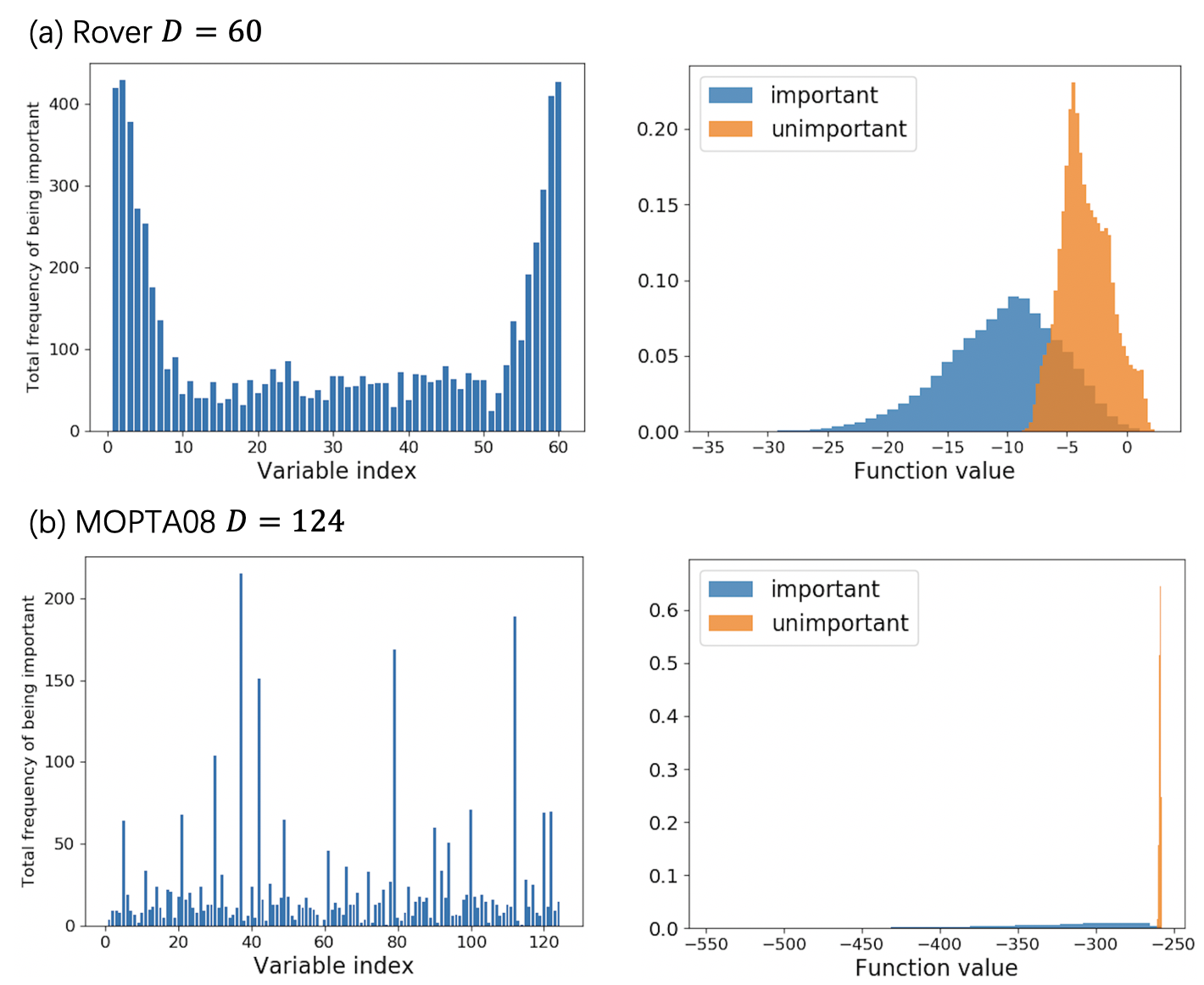
Figure 9: (left column) The total frequency of being chosen as important for each variable on the rover trajectory and MOPTA08 problems. (right column)The distribution of function values when sampling the first $5$ variables that have been chosen most frequently (important) or the first $5$ variables that have been chosen least frequently (unimportant) with all the other variables fixed.

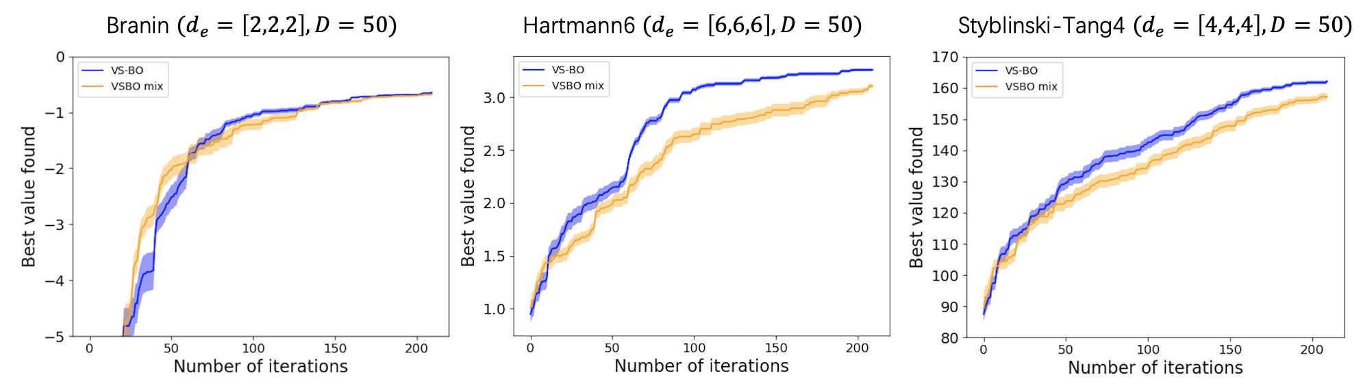
Figure 10: Performance of VS-BO and VSBO mix on Branin, Hartmann6 and Styblinski-Tang4 test functions. For each test function, we do 20 independent runs for each method. We plot the mean and 1/8 standard deviation of the best maximum value found by iterations.

References

- Auer [2002] Peter Auer. Using confidence bounds for exploitation-exploration trade-offs. Journal of Machine Learning Research, 3(Nov):397–422, 2002.
- Bergstra et al. [2013] James Bergstra, Daniel Yamins, and David Cox. Making a science of model search: Hyperparameter optimization in hundreds of dimensions for vision architectures. In International conference on machine learning, pages 115–123, 2013.
- Berkenkamp et al. [2016] Felix Berkenkamp, Andreas Krause, and Angela P Schoellig. Bayesian optimization with safety constraints: safe and automatic parameter tuning in robotics. arXiv preprint arXiv:1602.04450, 2016.
- Brochu et al. [2010] Eric Brochu, Vlad M Cora, and Nando De Freitas. A tutorial on Bayesian optimization of expensive cost functions, with application to active user modeling and hierarchical reinforcement learning. arXiv preprint arXiv:1012.2599, 2010.
- Calandra et al. [2016] Roberto Calandra, André Seyfarth, Jan Peters, and Marc Peter Deisenroth. Bayesian optimization for learning gaits under uncertainty. Annals of Mathematics and Artificial Intelligence, 76(1):5–23, 2016.
- Derksen and Keselman [1992] Shelley Derksen and Harvey J Keselman. Backward, forward and stepwise automated subset selection algorithms: Frequency of obtaining authentic and noise variables. British Journal of Mathematical and Statistical Psychology, 45(2):265–282, 1992.
- Djolonga et al. [2013] Josip Djolonga, Andreas Krause, and Volkan Cevher. High-dimensional Gaussian process bandits. In Advances in Neural Information Processing Systems, pages 1025–1033, 2013.