Power law decay of entanglement quantifiers in a single agent to a many body system coupling

Abstract

Manipulating many body quantum systems is a challenge. A useful way to achieve it would be to entangle the system to a diluted system, with a small particle number. Preparation of such entangled states can be facilitated as ground state of a many body Hamiltonian or the steady state of a many body open quantum system. Here we study two-site lattice models with a conserved boson number, biased to display a large occupancy in one of the sites. The Von Neumann entanglement entropy as well as the Logarithmic negativity show a typical power law decay in $R$, the occupancy ratio between the two sites. These results imply that it is feasible to entangle a large many body system to a single atom, as recently reported experimentally.

I Introduction

Entanglement is a key resource in quantum information Horodecki et al. (2009); Amico et al. (2008); Vedral (2018), quantum computing Nielsen and Chuang (2002); Preskill (2018) and quantum metrology Pezze et al. (2018). Recently, there has been significant advancement in generating, manipulating and measuring entangled many body states; both experimentally and theoretically Omran et al. (2019); Islam et al. (2015); Kaufman et al. (2016); Kallush et al. (2021). Both preparation of the entangled state and its validation using, e.g. entanglement witnesses Chruściński and Sarbicki (2014), are challenging aspects in many body systems and are the focus of ongoing research Lacroix (2020); Weimer et al. (2010); Carr and Saffman (2013); Verstraete et al. (2009).

Preparation of a desired entangled state can be realized as the ground state of a carefully designed Hamiltonian. Therefore, understanding the entanglement properties of ground states is of practical importance. Significant effort has been directed for extended systems, especially in $1D$. The ground state of a Hamiltonian with local interactions typically exhibits an area law in the bipartite Von Neumann entanglement entropy Eisert et al. (2008), contrary to the generic volume law of typical quantum states. However, the area law does not characterise a system composed of a few sites, where each site can occupy a large number of particles (see Fig. 1). For two sites, the average Von Neumann entanglement entropy is known Page (1993); Sen (1996), but the characteristic properties of the ground state entanglement remain largely unexplored.

A particularly appealing case is for a single agent in system $B$ to be entangled to a large number of particles in system $A$. Such entanglement allows to manipulate the many body system via the single agent. This setup was experimentally demonstrated in McConnell, R., Zhang, H., Hu, J. et al. (2015), where a single photon was entangled with roughly $3,000$ atoms. At this point, it is unknown whether there is a limit to the number of particles that could realistically be entangled with a single agent. It is further unknown whether our setup leads to typical ground state entanglement properties.

To answer the above questions, the entanglement needs to be quantified Friis et al. (2019); Plenio and Virmani (2007). Choosing an appropriate entanglement quantifier depends on the intended application, e.g. entanglement distillation to produce Bell states. However, the entanglement quantifier can alternatively be chosen to accommodate fast calculations of known density matrices, e.g. the Logarithmic negativity $E_{ln}$. For pure states, the Von Neumann entanglement entropy $E_{vn}$ serves both purposes.

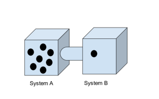
Figure 1: The systems $A$ and $B$ are made to interact such that we find a large occupancy of particles at system $A$ and a low occupancy at system $B$.

Keeping in mind the motivation of entangling a single agent to a many body system, we turn to a simpler theoretical setup. In this work we consider $N$ bosons, occupying a two-site system. We study the ground state entanglement properties when the system is tuned to display an overwhelming majority of bosons occupying site $A$ (see Fig. 1). To make this statement precise, let $\hat{n}_{A,B}$ be the corresponding number operators. Then, $R=\langle\hat{n}_{A}\rangle/\langle\hat{n}_{B}\rangle$ is the ratio of the particle occupancies. We study the large $R$ behaviour of both the ground state Von Neumann entanglement entropy and Logarithmic negativity of the Bose-Hubbard Hamiltonian. For open quantum systems, the same setup can be considered, where the steady state takes the role of the ground state. We study the steady state Logarithmic negativity of a Lindblad super-operator model – the quantum asymmetric inclusion process at large $R$ values Eisler (2011); Bernard et al. (2018).

Both models are studied at different scaling regimes. Nevertheless, they all consistently lead to a power law decay in the entanglement quantifiers. Quantitatively, the Von Neumann entanglement entropy $E_{vn}\sim\frac{\log R}{R^{\alpha}}$ and the Logarithmic negativity $E_{ln}\sim\frac{1}{R^{\alpha}}$ for $R\gg 1$. See Tables 1 and 2 for a summary of the results.

We argue that the power law decay is typical, as we have considered two disparate models and different scaling regimes for each model. The slow power law decay, contrasting with an exponential decay, answers in a quantifiable way how realistic it is to entangle a single, or a few atoms to a highly occupied many body state. The exponent $\alpha$ is non-universal. Therefore, interacting systems that result in small $\alpha$ values are favorable to facilitate entanglement between the diluted system to the large occupancy system.

The structure of this paper is as follows. In Sec. II we present the Hamiltonian and Lindblad models and summarise the main results. Sec. III presents in full the analytical and numerical treatment of the systems under study. Finally, Sec. IV recaps the main findings and their physical relevance and suggests future directions.

II Models and results

The aim of this work is to quantify the bipartite entanglement of a composite $AB$ system at large $R$ values. Therefore, it is natural to study lattice models, where the distinction between the two subsystems is clear cut. In particular, we study lattice models with two sites, $A$ and $B$.

To demonstrate the power law behaviour is typical, two disparate lattice models are considered. First, the ground state entanglement of the two-site Bose-Hubbard model is extensively studied. Second, we consider a generalization of the asymmetric inclusion process Grosskinsky et al. (2011) to the quantum realm via a Lindblad equation, dubbed here the quantum asymmetric inclusion process (QASIP). We then study the entanglement properties of the steady state at large $R$.

II.1 The two-site Bose-Hubbard model

The Bose-Hubbard model is a simple yet rich many body lattice model of spin-less bosons. It allows studying the superfluid-insulator transition Fisher et al. (1989) and can be experimentally implemented using optical lattices Jaksch et al. (1998); Greiner et al. (2002). The particular case of the two-site Bose-Hubbard model was extensively used in the literature to study tunneling effects between potential wells Links et al. (2006) as well as fragmentation Spekkens and Sipe (1999). Importantly for our purposes, the two site Bose-Hubbard model is expected to be both analytically tractable and to present typical physical behaviour in terms of the ground state entanglement. Hence, it serves as the starting point of our analysis.

The two-site Bose-Hubbard Hamiltonian is given by

$$H_{BH}=-J(\hat{b}^{\dagger}_{A}\hat{b}_{B}+\hat{b}^{\dagger}_{B}\hat{b}_{A})-\mu\hat{n}_{A}+\frac{U}{2}\sum_{i=A,B}\hat{n}_{i}-\hat{n}^{2}_{i},$$ (1)

where $J$ is the hopping matrix element between neighboring sites and $U$ determines the strength of the on-site interaction. The operators $\hat{b}_{i},\hat{b}^{\dagger}_{i}$ are the site-dependent bosonic creation and annihilation operators and $\hat{n}_{i}=\hat{b}^{\dagger}_{i}\hat{b}_{i}$ is the number operator for $i=A,B$. In an optical lattice, the potential wells are represented by the two sites Jaksch et al. (1998). The potential offset between the two asymmetric potential wells is given by $\mu$. It furthermore allows to imbalance the system towards large $R$ values.

It is useful to note that the total particle number, $\hat{N}=\hat{n}_{A}+\hat{n}_{B}$ is conserved. Therefore, we analyze the ground state with $N$ bosons. In what follows, we consider two scaling schemes leading to large $R$ values.

First, taking large $\mu$ values and keeping $N,J$ and $U$ fixed, a perturbative treatment leads to $R=\mu^{2}/J^{2}+O(\mu)$. See Sec. III. In this limit, and as long as $\frac{J\sqrt{N}}{\mu},\frac{UN^{2}}{\mu}\ll 1$, we find analytically the power law behaviour described in Table 1. These results are also numerically corroborated in Fig. 2. Note that the logarithmic correction in the Von Neumann entanglement hardly changes the behaviour from a clean power law.

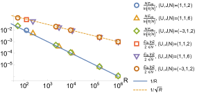
Figure 2: Corroborating the perturbation theory analytical predictions presented in Table 1. The entanglement quantifiers are evaluated numerically for the two-site Bose-Hubbard model and compared with perturbation theory. Different $U,J,N$ values are considered (see legend), in the range $\mu\in\left[10,10^{3}\right]$ to facilitate large $R$ values. No fitting parameters are required to observe the collapse onto the expected power law behaviour.

Second, we consider the large $N$ limit, with fixed $\mu,J$ and $U$. A perturbative approach is harder in this case as the Hilbert space of the effective Hamiltonian depends on the particle number $N$ (see Sec. III). See Fig. 3, Table 1 and the appendix C for the numerical analysis of the large $N$ limit.

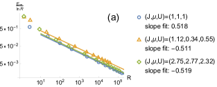
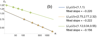
Figure 3: Numerical fitting of the entanglement quantifiers at the large $N$ limit of the two-site Bose-Hubbard model. Both $\frac{E_{vn}}{\log R}$ and $E_{ln}$ exhibit power law behaviour at large $R$ values, albeit with different exponents. Numerical convergence of arbitrary parameters to the same exponent is obtained when sufficiently large $R$ values are reached. (a) The Von Neumann entanglement entropy is shown to scale like $E_{vn}\propto\frac{\ln R}{R^{\alpha}}$, where $\alpha\approx 0.518$. The range $N\in\left[10,400\right]$ was tested. (b) The logarithmic negativity is shown to scale like $E_{ln}\propto R^{-\alpha}$, where $\alpha\approx 0.22$ is numerically fitted in the range $N\in\left[10,40\right]$. See the Appendix C for a detailed discussion on the reduced range of $N$ for the logarithmic negativity.

	$R$	$E_{vn}=\Gamma\frac{\ln R}{R^{\alpha}}$	$E_{ln}=\frac{\Gamma}{R^{\alpha}}$
$\mu\gg 1$	$\mu^{2}/J^{2}$	$\Gamma=N,\alpha=1$	$\Gamma=\frac{2\sqrt{N}}{\ln 2},\alpha=\frac{1}{2}$
$N\gg 1$	$\propto N^{\beta},\,\beta\approx 2.15$	$\alpha\approx 0.518$	$\alpha\approx 0.220$

Table 1: The power law behaviour of the ground state entanglement of the Bose-Hubbard model at large $R$ values. For the large $N$ limit, the exponents are evaluated numerically.

In conclusion, the ground state of the two-site Bose-Hubbard model leads to a power law behaviour of both the Von Neumann entanglement entropy and the Logarithmic negativity at large $R$ values in two different scaling schemes.

Next, we explore the large $R$ steady state entanglement in an open quantum system setup: the quantum asymmetric inclusion process.

II.2 Open quantum system

Realistically, physical systems are never truly isolated. Interestingly, the coupling of a quantum system to an environment does not always lead to complete loss of entanglement in the system. Indeed, there are examples where the environment can be engineered to produce a desirable entangled state Verstraete et al. (2009); Shpielberg (2020).

Here, we aim to study whether the large $R$ power law behaviour persists for steady states of open quantum systems as well. To that end, we focus on a quantum analog of the asymmetric inclusion process given in terms of the Lindblad equation.

In this setup, one usually assumes that a quantum system is coupled to an environment with fast relaxation times. This in turn, allows to discard non-Markovian contributions to the evolution of the density matrix and results in the Lindblad equation Petruccione, F. and Breuer, H.-P. (2002); Gorini et al. (1976); Lindblad (1976)

$$\partial_{t}\rho = \mathcal{H}(\rho)+\sum_{k}\mathcal{D}_{\hat{L}_{k}}(\rho)$$ (2)

$$\mathcal{H}(\rho) = -i\left[H,\rho\right]$$

$$\mathcal{D}_{\hat{L}}(\rho) = \hat{L}\rho\hat{L}^{\dagger}-\frac{1}{2}\{\hat{L}^{\dagger}\hat{L},\rho\}.$$

In eq.(2), $H$ is a Hermitian operator and $\left[\bullet,\bullet\right],\{\bullet,\bullet\}$ are the commutation and anti-commutation relations correspondingly. Despite the restriction to Markovian dynamics, enough quantumness remains in the Lindblad equation Spohn, Herbert and Lebowitz, Joel L. (1978); Kosloff, Ronnie (2013); Dutta and Cooper (2019). At this point, we turn to study a particular Lindblad model, allowing to facilitate the large $R$ limit analytically.

The QASIP describes the dynamics of bosons on a two-site lattice, where the boson interactions are environment assisted Eisler (2011); Bernard et al. (2018). The evolution of the density matrix is given by

$$\partial_{t}\hat{\rho} =\mathcal{L}_{QASIP}(\hat{\rho})$$ (3)

$$\mathcal{L}_{QASIP}(\hat{\rho}) =\mathcal{H}_{\mathrm{tb}}(\hat{\rho})+\mathcal{L}_{\mathrm{D}}(\hat{\rho})+\mathcal{L}_{E}(\hat{\rho})$$

$$H_{\mathrm{tb}}(\hat{\rho}) =\varepsilon\left(\hat{b}^{\dagger}_{A}\hat{b}_{B}+\hat{b}^{\dagger}_{B}\hat{b}_{A}\right)$$

$$\mathcal{L}_{\mathrm{D}}(\hat{\rho}) =\eta\sum_{k=A,B}\mathcal{D}_{\hat{n}_{k}}(\hat{\rho})$$

$$\mathcal{L}_{\mathrm{E}}(\hat{\rho}) =\gamma\mathcal{D}_{\hat{b}^{\dagger}_{A}\hat{b}_{B}}(\hat{\rho}).$$

See eq.(2) for the definition of $\mathcal{H},\mathcal{D}_{\hat{L}}$ for any operator $\hat{L}$. Here, the Hermitian $H_{\rm{tb}}$ is a tight-binding Hamiltonian inducing particle jumps between the two sites. $\mathcal{L}_{\mathrm{D}}$ is responsible for dephasing at each site and $\mathcal{L}_{\mathrm{E}}$ explicitly breaks the symmetry between the two sites and induces the occupation imbalance. Later on, it will be shown that controlling $\gamma$ allows to induce large $R$ values.

The relation of eq.(3) to the classical asymmetric inclusion process (ASIP) Grosskinsky et al. (2011) is as follows. The dephasing and bias terms alone acting on the diagonal terms of the density matrix in the number basis lead to the ASIP master equation. Namly, the quantum master equation is split to the diagonal terms and the coherent terms, each having a closed set of equations (in the number operator basis). The tight-binding Hamiltonian mixes between the cohrent terms and the diagonal terms, hence a quantum ASIP.

Three comments are in order before we present the results. First, note that here one cannot assume a priory that the quantum system is coupled to a series of thermalized baths as we have not performed a microscopic derivation of the Lindblad equation. Since we are not interested in studying thermalization, the lack of a microscopic derivation is of no importance. Second, the steady state density matrix is not pure. Hence, we will only use the Logarithmic negativity as an entanglement quantifier. Third, in eq.(3) we have set $\hbar$ to unity. Furthermore, we will assume $\varepsilon,\eta,\gamma$ and the time $t$ to be dimensionless for convenience. When presenting the different scaling schemes, the inverse time dimensions of $\varepsilon,\eta,\gamma$ could be restored.

The QASIP, like the Bose-Hubbard model can be shown to conserve the particle number $\hat{N}=\hat{n}_{A}+\hat{n}_{B}$ (see the appendix B). However, a related but more general property exists for the QASIP. In the number operator basis, we can write the density matrix as

$$\hat{\rho} = \sum_{S}a_{S}\hat{\rho}_{S},\quad\textrm{where}$$ (4)

$$\hat{\rho}_{S} = \sum^{S}_{x,y=0}\varrho_{S}(x,y)\ket{x,S-x}\bra{y,S-y}.$$

Here, $S$ takes non-negative integer values and $a_{S}$ are non-negative prefactors that sum to $1$. Note that the hermitianity of the density matrix $\hat{\rho}_{S}$ implies $\varrho^{*}_{S}(x,y)=\varrho_{S}(y,x)$ and unity trace implies $\sum^{S}_{x=0}\varrho_{S}(x,x)=1$.

The dynamics of eq.(3) is restricted to the subspace of $\hat{\rho}_{S}$:

$$\partial_{t}\varrho_{S}(x,y) = -\eta(x-y)^{2}\varrho_{S}(x,y)$$

$$+\gamma\,x_{-}y_{-}\varrho_{S}(x-1,y-1)$$

$$-\frac{1}{2}\gamma\left(x^{2}_{+}+y^{2}_{+}\right)\varrho_{S}(x,y)$$

$$-i\varepsilon\sum_{z=\pm 1}x_{z}\varrho_{S}(x+z,y)-y_{z}\varrho_{S}(x,y+z)$$

$$X_{+} = \sqrt{(X+1)(S-X)}$$

$$X_{-} = \sqrt{X(S-X+1)},\quad\textrm{where }X=x,y.$$

Namely, we have replaced the treatment of the infinite dimensional density matrix $\hat{\rho}$, with a treatment of finite dimensional $(S+1)^{2}$ density matrices $\hat{\rho}_{S}$ at fixed $S$.

The conserved number $S$ of $\hat{\rho}_{S}$ equals the number of particles in the system as

$$\Tr\hat{\rho}_{S}\hat{N}=\sqrt{\Tr\hat{\rho}_{S}\hat{N}^{2}}=S.$$ (6)

Eq.(II.2) implies therefore that the process conserves the particle number. From hereon out, we may replace $S$ by $N$.

In eq.(3), there are different scaling schemes leading to the large $R$ limit at the steady state. The Table 2 summarises the power law behaviour of the Logarithmic negativity in three different scaling regimes. The results in Table 2 were verified both analytically and numerically. See Fig. 4, for the large $\gamma$ limit and Fig. 5 for the large $\eta$ limit. For the large $N$ only numerical evidence is currently present, see Fig. 6 and 8.

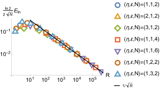
Figure 4: Corroborating the perturbation theory analytical predictions presented in Table 2. The Logarithmic negativity is evaluated numerically for the QASIP model and compared with perturbation theory at the large $\gamma$ limit in the range $\gamma\in\left[1,200\right]$. Different $\varepsilon,\eta,N$ values are considered, all showing the expected collapse onto the $1/\sqrt{R}$ plot at large $R$ values, with no fitting parameters.

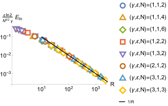
Figure 5: Corroborating the perturbation theory analytical predictions presented in Table 2. The Logarithmic negativity is evaluated numerically for the QASIP model and compared with perturbation theory at the large $\eta$ limit in the range $\eta\in\left[1,500\right]$. Different $\varepsilon,\gamma,N$ values are considered, all showing the expected collapse onto the $1/R$ plot at large $R$ values, with no fitting parameters.

	$R$	$E_{ln}(R)=\Gamma R^{-\alpha}$
$\gamma\gg 1$	$\frac{\gamma^{2}N^{2}}{4\varepsilon^{2}}$	$\Gamma=\frac{2\sqrt{N}}{\ln 2},\quad\alpha=1/2$
$\eta\gg 1$	$\eta\frac{N\gamma}{2\varepsilon^{2}}$	$\Gamma=\frac{2N^{3/2}\gamma}{\varepsilon\ln 2},\quad\alpha=1$
$N\gg 1$	$\propto N^{\beta},\beta\approx 1.988$	$\alpha\approx 0.236$

Table 2: The power law behaviour of the Logarithmic negativity in the steady state QASIP. For the large $N$ limit, the exponents are evaluated numerically.

In conclusion, the steady state QASIP in eq.(3) exhibits a power law decay in the Logarithmic negativity, similarly to the Bose-Hubbard dynamics.

In the next section, we provide a detailed derivation of the results for the Bose-Hubbard model and for the QASIP.

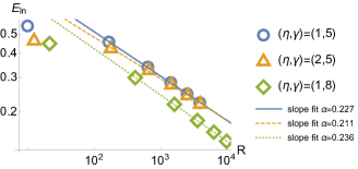
Figure 6: Numerical fitting of the Logarithmic negativity at the large $N$ limit of the QASIP model. Different $\eta,\gamma$ values were tested, leading to the large $R$ limit at $\varepsilon=1,N\in[1,25]$. Numerically, it is shown that $E_{ln}\propto R^{-\alpha}$, where $\alpha\approx 0.236$.

III Analytical and numerical analysis

In Sec. II, we have introduced two lattice models: the Bose-Hubbard model and the quantum asymmetric inclusion process. The power law behaviour of the Von Neumann entanglement and the Logarithmic negativity was summarized in Tables 1 and 2. In this section, we describe the analysis of these results in detail.

III.1 Bose-Hubbard model

To analyze the entanglement properties of the two-site Bose-Hubbard model in eq.(1), we need to find the $N$-particle ground state of the Hamiltonian. Given a description of the ground state, finding the ratio $R$ and the entanglement quantifiers $E_{vn},E_{ln}$ becomes straight-forward, but sometimes technically cumbersome. See the appendix A.

The Hilbert space of $N$ particles for the Bose-Hubbard Hamiltonian eq.(1) is spanned by the $N+1$ Fock states $\ket{n_{A},n_{B}}=\frac{1}{n_{A}!n_{B}!}(\hat{b}^{\dagger}_{A})^{n_{A}}(\hat{b}^{\dagger}_{B})^{n_{B}}\ket{0,0}$. Namely,

$$\ket{\psi_{N}}=\sum^{N}_{k=0}a_{k}\ket{k,N-k},\quad\textrm{where }\sum^{N}_{k=0}|a_{k}|^{2}=1.$$ (7)

Then, the $N$ particle Bose-Hubbard Hamiltonian can be written as a $N+1\times N+1$ matrix. Finding the ground state can be done analytically and for all $\mu,U,J$ values when we set $N=1$. This simple case will reveal the intuitive scaling limits leading to the large $R$ behaviour, both for the Bose-Hubbard model as well as for the quantum asymmetric inclusion process in the next subsection.

Indeed, for $N=1$, the Bose-Hubbard Hamiltonian can be represented by the $2\times 2$ matrix

$$H^{(N=1)}_{BH}=\begin{pmatrix}-\mu&-J\\ -J&0,\end{pmatrix}$$ (8)

where the wavefunction is in its most general form

$$\ket{\psi_{N=1}}=\cos\zeta\ket{10}+{\rm e}^{i\phi_{1}}\sin\zeta\ket{01}=\begin{pmatrix}\cos\zeta\\ {\rm e}^{i\phi_{1}}\sin\zeta\end{pmatrix}$$ (9)

for real $\zeta,\phi_{1}$ values and the right hand side of eq.(9) is in a vector notation corresponding to the matrix in eq.(8). Clearly, the ratio is $R=\cot^{2}\zeta$. The lowest eigenvalue of eq.(8) is $\epsilon=-\frac{1}{2}(\mu+\sqrt{\mu^{2}+4J^{2}})$ with the ground state $\ket{\psi_{N=1}}=\frac{1}{\mathcal{N}}(-\epsilon\ket{10}+J\ket{01})$ and $\mathcal{N}^{2}=\epsilon^{2}+J^{2}$ is a normalization constant. This implies that $R=\epsilon^{2}/J^{2}$. Therefore, in this particular case, $R\gg 1$ only if $\mu/J\gg 1$ and leads to $R=(\mu/J)^{2}+O(\mu)$ asymptotically.

The Von Neumann entanglement for the ground state in eq.(9) is

$$E_{vn}=-2\cos^{2}\zeta\ln(\cos\zeta)-2\sin^{2}\zeta\ln(\sin\zeta).$$ (10)

Using trigonometric identities, we recover $\cos^{2}\zeta=\frac{R}{1+R}$ and $\sin^{2}\zeta=\frac{1}{1+R}$. Asymptotically for large $R$, $E_{vn}=\frac{\ln R}{R}$ to leading order as reported in Table 1.

To find the Logarithmic negativity, we need to write the partially transposed density matrix

$$\rho^{PT} = \cos^{2}\zeta\ket{10}\bra{10}+\sin^{2}\zeta\ket{01}\bra{01}$$

$$+\cos\zeta\sin\zeta\left({\rm e}^{i\phi_{1}}\ket{00}\bra{11}+{\rm e}^{-i\phi_{1}}\ket{11}\bra{00}\right).$$

The eigenvalues of the partially transposed density matrix are $\cos^{2}\zeta,\sin^{2}\zeta$ and $\pm\frac{\sqrt{1-\cos 4\zeta}}{2\sqrt{2}}$. Therefore, the Logarithmic negativity is $E_{ln}=\log_{2}(1+\frac{\sqrt{1-\cos 4\zeta}}{\sqrt{2}})$. For large $R$ and to leading order, we find $E_{ln}=\frac{2}{\ln 2}R^{-1/2}+O(R^{-1})$ as reported in Table 1.

For $N>1$, the ground state solution becomes cumbersome, but still requires dealing with a $N+1\times N+1$ Bose-Hubbard matrix. The numerical code that produced Fig. 2,3 and 7 finds the ground state of the Bose-Hubbard matrix at some finite $N$. Then, it calculates the Von Neumann entanglement and the Logarithmic negativity.

From the $N=1$ example , we have seen that the large $\mu$ limit leads to a large bias $R\gg 1$. This happens when the $\mu$ term dominates the energy of the ground state, i.e. for $\mu\gg\sqrt{N}J,UN^{2}$. Another large $R$ limit is recovered for finite $\mu,U,J>0$ and large $N$. In this limit, the particles condense due to the strong attractive energy $\sim UN^{2}$. The symmetry is broken by the potential offset $\mu$, leading to condensation of the particles in site $A$ and to large $R$ values.

A perturbative approach for the large $N$ limit is non-trivial due to as the dimension of the effective Hilbert space changes with $N$. However, a direct numerical analysis clearly reveals the power law behaviour in this limit. See Table 1, Sec.II and the appendix C for more details. In what follows, we consider the large $\mu$ limit and evaluate the ground state and the entanglement quantifiers using a perturbative approach.

Let us develop a standard perturbation theory for the Hamiltonian $H=H_{0}+\frac{1}{\mu}H_{1}{\color[rgb]{0,0,0}=\frac{1}{\mu}H_{BH}}$

$$H_{0}=-\hat{n}_{A}\quad H_{1}=H_{BH}-\mu H_{0},$$ (12)

at large $\mu$.

The eigenstates of $H_{0}$ are $\ket{\phi^{(0)}_{n}}=\ket{n,N-n}$ with energies $\epsilon^{(0)}_{n}=-n$. The first order correction to the ground state is

$$\ket{\phi_{N}}=\ket{N,0}+\lambda\ket{N-1,1}+O(\lambda^{2})$$ (13)

where $\lambda=\frac{J\sqrt{N}}{\mu}$ assumed to be small as well as $UN^{2}/\mu\ll 1$. At this limit we find $R=\langle\hat{n}_{A}\rangle/\langle\hat{n}_{B}\rangle=N/\lambda^{2}.$ So, we can approximate at small $\lambda$, $R=\mu^{2}/J^{2}+O(\mu)$. The Von Neumann entanglement can be calculated for the ground state $\ket{\phi_{N}}$

$$E_{vn}=-\frac{1}{1+\lambda^{2}}\ln\frac{1}{1+\lambda^{2}}-\frac{\lambda^{2}}{1+\lambda^{2}}\ln\frac{\lambda^{2}}{1+\lambda^{2}}$$ (14)

$$=-\lambda^{2}\ln\lambda^{2}+O(\lambda^{3}).$$

At this limit, we find the reported scaling

$$E_{vn}=\frac{N}{R}\ln\frac{N}{R}$$ (15)

to leading order. This is corroborated numerically in Fig. 2 and summarised in Table 1. Recall that in this scaling, $N$ may be large, but $R\gg N$.

To find the Logarithmic negativity, we need to calculate the eigenvalues of the partially transposed density matrix of $\ket{\phi_{N}}$. For $N>1$, the only non-zero eigenvalues are $\frac{1}{1+\lambda^{2}},\frac{\lambda^{2}}{1+\lambda^{2}},\frac{\pm\lambda}{1+\lambda^{2}}$. This leads to

$$E_{ln}=\log_{2}\left(1+\frac{2\lambda}{1+\lambda^{2}}\right)=\frac{2}{\ln 2}\sqrt{\frac{N}{R}}+O(1/R).$$ (16)

For large $R$ values, where the perturbation theory applies, the Logarithmic negativity dominates the Von Neumann entanglement as it should Plenio and Virmani (2007); Plenio et al. (2005). Again, we refer to Fig. 2 to see the excellent agreement with the numerical evaluation.

Other scaling schemes, leading to large $R$ values can exist. Nevertheless, the power law behaviour of the entanglement quantifiers is believed to persist, based on the $N=1$ exactly solvable cases.

We turn to study the large $R$ entanglement properties of a completely different setup – the quantum asymmetric inclusion process.

III.2 The QASIP

To analyze the steady state entanglement properties of the QASIP at large $R$, we need to find the steady state density matrix with a fixed $S$, i.e. $\mathcal{L}_{QASIP}(\hat{\rho}_{S})=0$. Namely, we wish to find $\varrho_{S}(x,y)$ such that the right hand side of eq.(II.2) vanishes.

As in the Bose-Hubbard model, it is useful to study first the simple case of $S=1$. Here, $x,y=\{0,1\}$ and demanding a steady state in eq.(II.2) leads to

$$\begin{pmatrix}-\gamma&i\varepsilon&-i\varepsilon&0\\ i\varepsilon&-\frac{1}{2}\gamma-\eta&0&-i\varepsilon\\ -i\varepsilon&0&-\frac{1}{2}\gamma-\eta&i\varepsilon\\ \gamma&-i\varepsilon&i\varepsilon&0\end{pmatrix}\begin{pmatrix}\varrho_{1}(0,0)\\ \varrho_{1}(0,1)\\ \varrho_{1}(1,0)\\ \varrho_{1}(1,1)\end{pmatrix}=\begin{pmatrix}0\\ 0\\ 0\\ 0\end{pmatrix}.$$ (17)

Solving eq.(17), we find the steady state solution for $S=1$

$$\mathcal{N}_{1}\hat{\rho}_{1} = 4\varepsilon^{2}\ket{0,1}\bra{0,1}$$

$$+2i\gamma\varepsilon\left(\ket{1,0}\bra{0,1}-\ket{0,1}\bra{1,0}\right)$$

$$+(4\varepsilon^{2}+\gamma^{2}+2\gamma\eta)\ket{1,0}\bra{1,0}.$$

where $\mathcal{N}_{1}=\gamma^{2}+2\gamma\eta+8\varepsilon^{2}$ ensures unity trace of $\hat{\rho}_{1}$. From the steady state solution we recover $R=1+\frac{\gamma(\gamma+2\eta)}{4\varepsilon^{2}}$ and $E_{ln}=\log_{2}\left(1+\frac{4\gamma\varepsilon}{\gamma^{2}+8\varepsilon^{2}+2\gamma\eta}\right)$. A few observations can already be made. At $\eta\rightarrow\infty$ the entanglement vanishes as can be expected in the large dephasing limit Bernard et al. (2018); Fischer et al. (2016). Moreover, the Logarithmic negativity becomes positive due to a combination of biasing and coherent hopping, i.e. $\gamma\varepsilon>0$. We identify two limits where $R$ becomes large. For $\gamma\rightarrow\infty$ and finite $\eta,\varepsilon$ we recover $R\propto\gamma^{2}$ and $E_{ln}\propto 1/\sqrt{R}$. Similarly, for finite $\gamma,\varepsilon$ and large $\eta$ we recover $R\propto\eta$ and $E_{ln}\propto 1/R$. Already for the $S=1$ case we find that the entanglement power law behavior persists for large $R$ values. However, the exponent is non-universal and depends on the scaling scheme.

Exact solution of the steady state for $S>1$ is at best tedious. Instead, we will find the steady state solution at the two limits noted above, using a perturbative approach; The limits at finite $S$ will be shown to agree with the $S=1$ exact analysis carried out in the above.

III.2.1 Large asymmetry between the sites

For $\gamma\gg 1$, and at finite $S,\eta,\varepsilon$, we develop the steady state density matrix as a perturbative sum

$$\hat{\rho}_{S}=\frac{1}{\mathcal{N}_{\gamma}}(\hat{\rho}^{(0)}_{S}+\frac{1}{\gamma}\hat{\rho}^{(1)}_{S}+\frac{1}{\gamma^{2}}\hat{\rho}^{(2)}_{S})+O(1/\gamma^{3}),$$ (19)

where $\mathcal{N}_{\gamma}$ is a normalization constant to assure trace one of the truncated density matrix. This perturbative approach implies the order by order steady state solutions

$$0 = \mathcal{L}_{\mathrm{E}}(\hat{\rho}^{(0)}_{S})$$ (20)

$$0 = \frac{1}{\gamma}\mathcal{L}_{\mathrm{E}}(\hat{\rho}^{(1)}_{S})+(\mathcal{L}_{\mathrm{D}}+\mathcal{H}_{tb})\hat{\rho}^{(0)}_{S}$$ (21)

$$0 = \frac{1}{\gamma}\mathcal{L}_{\mathrm{E}}(\hat{\rho}^{(2)}_{S})+(\mathcal{L}_{\mathrm{D}}+\mathcal{H}_{tb})\hat{\rho}^{(1)}_{S}$$ (22)

Eq.(20) admits a uniqe solution $\hat{\rho}^{(0)}_{S}=\ket{S,0}\bra{S,0}$, namely to leading order site $A$ is maximally occupied and site $B$ is depleted. Using the leading order solution, we find $\hat{\rho}^{(1)}_{S}=\frac{2i\varepsilon}{\sqrt{S}}(\ket{S,0}\bra{S-1,1}+\ket{S-1,1}\bra{S,0})$. Note that to first order, there are yet no corrections to the occupancies. Hence, we solve to second order in $1/\gamma$ obtaining

$$\hat{\rho}^{(2)}_{S} = \frac{4\varepsilon^{2}}{\gamma^{2}S}\ket{S-1,1}\bra{S-1,1}$$

$$+ \frac{4i\varepsilon\eta}{S^{3/2}}\ket{S-1,1}\bra{S,0}$$

$$- \frac{2\sqrt{2}\varepsilon^{2}}{\sqrt{S(S-1)}}\ket{S,0}\bra{S-2,2}+\textrm{h.c.}.$$

To second order, we find $\mathcal{N}_{\gamma}=\frac{4\varepsilon^{2}}{\gamma^{2}S}+1$. From the perturbative solution of eq.(19), we find that

$$R=S-1+\frac{S^{2}\gamma^{2}}{4\varepsilon^{2}}+O(\gamma)\approx\frac{S^{2}\gamma^{2}}{4\varepsilon^{2}}.$$ (24)

This approximation also implies the assumption $\varepsilon^{2}\ll S\gamma^{2}$. Also, the Logarithmic negativity can be calculated as there are at most four non-zero eigenvalue for partially transposed density matrix for any $S$ value. We find to leading order

$$E_{ln}=\frac{4\varepsilon}{\gamma\sqrt{S}\ln 2}+O(\frac{1}{\gamma^{2}})\approx\frac{2\sqrt{S}}{\ln 2}\frac{1}{\sqrt{R}}+O(\frac{1}{R}).$$ (25)

As noted in Sec. II, the $E_{ln}(R)$ power law behaviour was verified numerically in Fig. 4.

III.2.2 Large dephasing limit

Here we consider the large $\eta$ limit with fixed $S,\gamma,\varepsilon$. We write the density matrix as a perturbative series in $1/\eta$

$$\hat{\rho}_{S}=\frac{1}{\mathcal{N}_{\eta}}(\hat{\rho}^{(0)}_{S}+\frac{1}{\eta}\hat{\rho}^{(1)}_{S}+\frac{1}{\eta^{2}}\hat{\rho}^{(2)}_{S})+O(1/\eta^{3}),$$ (26)

where here $\mathcal{N}_{\eta}$ is a normalization constant ensuring the truncated density matrix has trace $1$. Again, the perturbative series implies the order by order steady state solutions

$$0= \mathcal{L}_{\mathrm{D}}(\hat{\rho}^{(0)}_{S})$$ (27)

$$0= \frac{1}{\eta}\mathcal{L}_{\mathrm{D}}(\hat{\rho}^{(1)}_{S})+(\mathcal{L}_{\mathrm{E}}+\mathcal{H}_{tb})\hat{\rho}^{(0)}_{S}$$ (28)

$$0= \frac{1}{\eta}\mathcal{L}_{\mathrm{D}}(\hat{\rho}^{(2)}_{S})+(\mathcal{L}_{\mathrm{E}}+\mathcal{H}_{tb})\hat{\rho}^{(1)}_{S}$$ (29)

Eq.(27) admits a degenerate solution

$$\hat{\rho}^{(0)}_{S}=\sum^{S}_{k=0}a_{k}\ket{k,S-k}\bra{k,S-k}$$ (30)

with $a_{k}$ non-negative coefficients. This degeneracy is broken in the next order, i.e. eq.(28). We find $\hat{\rho}^{(0)}_{S}=\ket{S,0}\bra{S,0}$, however the degeneracy moves to the next order

$$\hat{\rho}^{(1)}_{S}= \sum^{S}_{k=0}b_{k}\ket{k,S-k}\bra{k,S-k}$$ (31)

$$+ i\varepsilon\sqrt{S}(\ket{S,0}\bra{S-1,1}-\ket{S-1,1}\bra{S,0}),$$

where $b_{k}$ are again non-negative coefficients. To evaluate to leading order $R$, we have to break the degeneracy in $b_{k}$. This breaking is obtained at the next order, i.e. eq.(29), where we find $b_{k}=\delta_{k,S-1}\frac{2\varepsilon^{2}}{\gamma}$ and

$$\hat{\rho}^{(2)}_{S}= -\frac{\varepsilon^{2}\sqrt{S-1}\sqrt{S}}{2\sqrt{2}}\ket{S-2,2}\bra{S,0}$$

$$+ i\frac{\gamma^{2}\varepsilon S^{3/2}+4\varepsilon^{3}\sqrt{S}}{2\gamma}\ket{S-1,1}\bra{S,0}$$

$$- i\frac{2\sqrt{2}\varepsilon^{3}\sqrt{S-1}}{\gamma}\ket{S-2,2}\bra{S-1,1}$$

$$+ \sum^{S}_{k=0}c_{k}\ket{k,S-k}\bra{k,S-k}$$

$$+\textrm{h.c.}.$$ (32)

The degeneracy in the non-negative terms $c_{k}$ is broken at the third order of the expansion. To leading order in $\eta$, we find $\mathcal{N}_{\eta}=1+\frac{2\varepsilon^{2}}{\gamma\eta}$. Therefore, to leading order

$$R=\frac{\gamma\eta S}{2\varepsilon^{2}}+S-1\approx\frac{\gamma\eta S}{2\varepsilon^{2}}.$$ (33)

Again, the spectrum of the partially transposed density matrix is composed of only four non-zero eigenvalues for any $S>1$: $(-\frac{\gamma\varepsilon\sqrt{S}}{\gamma\eta+2\varepsilon^{2}},\frac{\gamma\varepsilon\sqrt{S}}{\gamma\eta+2\varepsilon^{2}},\frac{2\varepsilon^{2}}{\gamma\eta+2\varepsilon^{2}},\frac{\gamma\eta}{\gamma\eta+2\varepsilon^{2}})$. The Logarithmic negativity is thus given by

$$E_{\ln}=\log_{2}\left(1+\frac{2\gamma\varepsilon\sqrt{S}}{\gamma\eta+2\varepsilon^{2}}\right)\approx\frac{2\varepsilon\sqrt{S}}{\eta\ln 2}=\frac{\gamma S^{3/2}}{\varepsilon\ln 2}\frac{1}{R}.$$ (34)

As noted in Sec. II, the $E_{ln}(R)$ power law behaviour was verified numerically in Fig. 5.

III.3 Large number of particles

We also studied the scaling limit $S\gg 1$ and finite $\eta,\gamma,\varepsilon$. Analytically, a perturbative solution in this case becomes hard due to the change in the state space, similarly to the Bose-Hubbard case. Nevertheless, it is possible to numerically find the steady state and calculate the Logarithmic negativity even for large $S$ values. This was carried out numerically (Fig. 6) and reported on in Sec. II.

IV Discussion

State of the art experimental techniques allows to entangle a single agent to thousands of atoms McConnell, R., Zhang, H., Hu, J. et al. (2015). However, it was unclear whether one could push the experimental techniques to significantly increase the number of atoms entangled to the agent.

Here, we have explored the theoretical bounds on entangling one or a few agents to a many body system. The ground state of a two-site Bose-Hubbard model, with an occupancy bias $R\gg 1$ leads to a power law decay in the Logarithmic negativity and the Von Neumann entanglement entropy in different scaling limits. Furthermore, the steady state of the QASIP biased to large $R$ values also exhibits a power law decay in the Logarithmic negativity. We stress that while the power law behaviour is typical, the exponent depends on the scaling limits, see Tables 1 and 2.

From the slow decay of the entanglement, it is now clear it is typically possible to entangle thousands of atoms to a single agent. Furthermore, designing systems with slow entanglement decay (small $\alpha$) allows to entangle more particles in the many body system to the one agent (or a few). It would be particularly appealing to develop a perturbative approach to the large $N$ limit in both models. Such an approach would allow to extract the exponents analytically, explore their range and dependence on the model parameters. Furthermore, it would suggest how best to tune the parameters to entangle the diluted system $B$ to the highly occupied system $A$.

The average Von Neumann entanglement entropy over the random pure state of Hilbert space $N\times N$ is $E_{vn}\sim\log N$ Page (1993); Sen (1996). Therefore, the Von Neumann entanglement entropy of the ground state is fundamentally different than that of the average. This is not too surprising when one relates to the area law of ground states in extended systems compared to the typical volume law. In turn, the low Von Neumann entanglement entropy of the ground state suggests that ground states in the large $R$ limit could be susceptible to analytical and numerical techniques, even for large many body systems.

From the analysis so far, it may seem that the two-site lattice model is paramount to achieve the power law behaviour. We have carried out preliminary tests in a three site Hubbard model. Taking sites $A,B$ to occupy most of the particles in the system, namely $R=\langle\hat{n}_{A}+\hat{n}_{B}\rangle/\langle\hat{n}_{C}\rangle$. The Von Neumann entanglement entropy between site $C$ and the subsystem $AB$ still exhibits a power law in large $R$. The analysis is beyond the scope of this work and will be presented elsewhere.

Another question that comes to mind is whether the power law behaviour persists also in continuum models, and not only in lattice models. We believe this is not the case. After coarse graining a lattice model into a continuum model, an increase is expected in the Von Neumann entanglement entropy due to loss of information. This increase does not depend on the occupancies and hence adds a constant to the Von Neumann entanglement entropy. Therefore, in the large $R$ limit we expect to observe a saturation to a constant with a power law correction. Naively, that should be the same power law of the lattice model. It would be interesting to test this conjecture in future works.

Acknowledgments: I would like to thank Guy Cohen, Shahaf Asban and Ofir E. Alon for stimulating talks on the subject.

Appendix A Entanglement quantifiers

In this section, we provide a brief introduction to the entanglement quantifiers used in this text: the Von Neumann entanglement entropy and the Logarithmic negativity. The purpose of quantifiers is to distinguish between entangled to non-entangled states (separable) and furthermore to suggest a hierarchy of values for entangled states. Here we do not aim to give an exhaustive account of quantum quantifiers, but to motivate the usage of the Von Neumann entanglement entropy and the Logarithmic negativity in the case at hand.

For pure states, all entanglement measures are defined to correspond to the Von Neumann entanglement entropy Plenio and Virmani (2007). In bipartite system $AB$,

$$E_{vn}(\rho_{AB})=-\Tr\rho_{A}\ln\rho_{A}=-\Tr\rho_{B}\ln\rho_{B},$$ (35)

where $\rho_{A}=\Tr_{B}\rho_{AB}$ is the reduced density matrix. $E_{vn}>0$ only for non-separable pure states.

In terms of wave functions (which are pure states), the Schmidt decomposition using orthonormal states imply $\ket{\psi}=\sum_{i}\alpha_{i}\ket{u_{i}}_{A}\otimes\ket{v_{i}}_{B}$. Then, we find $E_{vn}(\ket{\psi})=-\sum_{i}|\alpha_{i}|^{2}\log|\alpha_{i}|^{2}$.

Entanglement is harder to quantify for mixed states. Many different measures for the entanglement exists. Typically, entanglement measures are given in the form of some minimization problem, making them hard to calculate. Instead, we will use the Logarithmic negativity which is an entanglement monotone and not a measure. Namely, for pure state the Logarithmic negativity does not correspond to the Von Neumann entanglement entropy (except for specific cases). However, it is straight-forward to calculate the Logarithmic negativity, making it a favorable entanglement quantifier.

The Logarithmic Negativity is given by

$$E_{ln}(\rho)=\log_{2}\lVert\rho^{PT}\rVert_{1},$$ (36)

where $\rho^{PT}$ is the partially transposed density matrix, and $\lVert A\rVert_{1}\equiv\Tr\sqrt{AA^{\dagger}}$. Intuitively speaking, the Logarithmic negativity counts the amount of negative eigenvalues in the partially transposed density matrix relating it to the Peres–Horodecki criterion Peres (1996); Horodecki et al. (1996). We note that a positive Logarithmic negativity values insures non-separability, but a vanishing value does not guarantees separability.

The Logarithmic Negativity is an entanglement monotone Plenio (2005); Plenio and Virmani (2007); Friis et al. (2019), which implies that on average, under locally quantum operations and classical communication (LOCC), the Logarithmic Negativity does not increase. Furthermore, the Logarithmic negativity was shown to be an upper bound for the distillation entanglement, connecting it to useful quantum operations using maximally entangled states Audenaert et al. (2003). Since the distillation entanglement is an entanglement measure, it is evident that for pure states, the Von Neumann entanglement entropy is bounded by the Logarithmic negativity. This fact provides a consistency check in our numerical assessment.

Appendix B The Lindblad adjoint dynamics

The purpose of this section is to introduce the Heisenberg operator evolution picture for the Lindblad dynamics.

For an observable $\hat{O}$ (explicitly time-independent), we have the expectation value $\langle\hat{O}\rangle=\Tr\hat{O}\rho$. Therefore,

$$\partial_{t}\langle\hat{O}\rangle=\Tr\hat{O}\partial_{t}\rho=\Tr\hat{O}\mathcal{L}(\rho),$$ (37)

where $\mathcal{L}(\rho)$ is a Lindblad super-operator of eq.(2). Then, the formal adjoint $\mathcal{L}^{\dagger}$ is defined such that

$$\partial_{t}\langle\hat{O}\rangle=\Tr\mathcal{L}^{\dagger}(\hat{O})\rho.$$ (38)

For the Lindblad super-operator in eq.(2), it implies the Heisenberg picture

$$\partial_{t}\hat{O}=\mathcal{L}^{\dagger}(\hat{O})=-\mathcal{H}(\hat{O})+\sum_{k}\hat{L}^{\dagger}_{k}\hat{O}\hat{L}_{k}-\frac{1}{2}\{\hat{L}^{\dagger}_{k}\hat{L}_{k},\hat{O}\}.$$ (39)

It is rather straight-forward to see that $\partial_{t}\hat{N}=0$ for the QASIP.

Appendix C Additional numerical data for the Bose-Hubbard model

Here we present further technical details on the numerical analysis of the Bose-Hubbard model.

For large $N$ values, the Von Neumann entanglement entropy is easier to obtain than the logarithmic negativity. In the Appendix A, it was shown that the pure state Von Neumann entanglement entropy can be obtained from the ket state. However, the logarithmic negativity requires finding the spectrum of the partially transposed density matrix. The complexity of handling density matrices is certainly higher than that of handling ket states, hence the lower values that were reached for the logarithmic negativity.

In Fig. 7 the scaling $R\propto N^{\beta}$ is presented in the large $N$ limit for three values of the parameters $(J,U,\mu)$. The values are picked to produce large $R$ values and to span over a few length scales in $R$, providing a reliable prediction for the exponents.

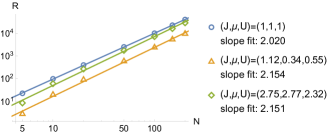
Figure 7: In the large $N$ limit of the two-site Bose-Hubbard model, numerical evaluation show that $R\propto N^{\beta}$ with $\beta\approx 2.15$. The three parameters in the range $N\in\left[1,400\right]$, are picked to allow for a sufficiently large $R$ values.

Appendix D Additional numerical data for the QASIP model

Here we present further technical details on the numerical analysis of the QASIP model.

In Fig. 8 the large $N$ scaling of $R\propto N^{\beta}$ is plotted for different $\gamma$ values. Since testing the logarithmic negativity in large $N$ values is numerically challenging, the parameters were chosen to facilitate as large $R$ as possible which improves exponent fitting.

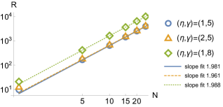
Figure 8: In the large $N$ limit of the QASIP model, it is numerically corroborated that $R\propto N^{\beta}$ where $\beta\approx 1.988$. Different $\eta,\gamma$ values were tested, leading to the large $R$ limit at $\varepsilon=1,N\in[1,25]$.

References

- Horodecki et al. (2009) R. Horodecki, P. Horodecki, M. Horodecki, and K. Horodecki, Rev. Mod. Phys. 81, 865 (2009).
- Amico et al. (2008) L. Amico, R. Fazio, A. Osterloh, and V. Vedral, Reviews of modern physics 80, 517 (2008).
- Vedral (2018) V. Vedral, Decoding reality: the universe as quantum information (Oxford University Press, 2018).
- Nielsen and Chuang (2002) M. A. Nielsen and I. Chuang, “Quantum computation and quantum information,” (2002).
- Preskill (2018) J. Preskill, Quantum 2, 79 (2018).
- Pezze et al. (2018) L. Pezze, A. Smerzi, M. K. Oberthaler, R. Schmied, and P. Treutlein, Reviews of Modern Physics 90, 035005 (2018).
- Omran et al. (2019) A. Omran, H. Levine, A. Keesling, G. Semeghini, T. T. Wang, S. Ebadi, H. Bernien, A. S. Zibrov, H. Pichler, S. Choi, et al., Science 365, 570 (2019).
- Islam et al. (2015) R. Islam, R. Ma, P. M. Preiss, M. E. Tai, A. Lukin, M. Rispoli, and M. Greiner, Nature 528, 77 (2015).
- Kaufman et al. (2016) A. M. Kaufman, M. E. Tai, A. Lukin, M. Rispoli, R. Schittko, P. M. Preiss, and M. Greiner, Science 353, 794 (2016).
- Kallush et al. (2021) S. Kallush, R. Dann, and R. Kosloff, arXiv preprint arXiv:2107.11767 (2021).
- Chruściński and Sarbicki (2014) D. Chruściński and G. Sarbicki, Journal of Physics A: Mathematical and Theoretical 47, 483001 (2014).
- Lacroix (2020) D. Lacroix, Physical Review Letters 125, 230502 (2020).
- Weimer et al. (2010) H. Weimer, M. Müller, I. Lesanovsky, P. Zoller, and H. P. Büchler, Nature Physics 6, 382 (2010).
- Carr and Saffman (2013) A. Carr and M. Saffman, Physical Review Letters 111, 033607 (2013).
- Verstraete et al. (2009) F. Verstraete, M. M. Wolf, and J. I. Cirac, Nature physics 5, 633 (2009).
- Eisert et al. (2008) J. Eisert, M. Cramer, and M. B. Plenio, arXiv preprint arXiv:0808.3773 (2008).
- Page (1993) D. N. Page, Physical Review Letters 71, 1291 (1993).
- Sen (1996) S. Sen, Physical Review Letters 77, 1 (1996).
- McConnell, R., Zhang, H., Hu, J. et al. (2015) McConnell, R., Zhang, H., Hu, J. et al. , Nature 519, 439–442 (2015).
- Friis et al. (2019) N. Friis, G. Vitagliano, M. Malik, and M. Huber, Nat. Rev. Phys. 1, 72 (2019).
- Plenio and Virmani (2007) M. B. Plenio and S. Virmani, Quant.Inf.Comput 7 (2007).
- Eisler (2011) V. Eisler, Journal of Statistical Mechanics: Theory and Experiment 2011, P06007 (2011).
- Bernard et al. (2018) D. Bernard, T. Jin, and O. Shpielberg, EPL (Europhysics Letters) 121 (6), 60006 (2018).
- Grosskinsky et al. (2011) S. Grosskinsky, F. Redig, and K. Vafayi, J. Stat. Phys. 142, 952 (2011).
- Fisher et al. (1989) M. P. A. Fisher, P. B. Weichman, G. Grinstein, and D. S. Fisher, Phys. Rev. B 40, 546 (1989).
- Jaksch et al. (1998) D. Jaksch, C. Bruder, J. I. Cirac, C. W. Gardiner, and P. Zoller, Physical Review Letters 81, 3108 (1998).
- Greiner et al. (2002) M. Greiner, O. Mandel, T. Esslinger, T. W. Hänsch, and I. Bloch, nature 415, 39 (2002).
- Links et al. (2006) J. Links, A. Foerster, A. P. Tonel, and G. Santos, in Annales Henri Poincaré, Vol. 7 (Springer, 2006) pp. 1591–1600.
- Spekkens and Sipe (1999) R. Spekkens and J. Sipe, Physical Review A 59, 3868 (1999).
- Shpielberg (2020) O. Shpielberg, EPL (Europhysics Letters) 129, 60005 (2020).
- Petruccione, F. and Breuer, H.-P. (2002) Petruccione, F. and Breuer, H.-P., The Theory of Open Quantum Systems (Oxford University Press, 2002).
- Gorini et al. (1976) V. Gorini, A. Kossakowski, and E. C. G. Sudarshan, Journal of Mathematical Physics 17, 821 (1976).
- Lindblad (1976) G. Lindblad, Communications in Mathematical Physics 48, 119 (1976).
- Spohn, Herbert and Lebowitz, Joel L. (1978) Spohn, Herbert and Lebowitz, Joel L., J. Adv. Chem. Phys 38, 109 (1978).
- Kosloff, Ronnie (2013) Kosloff, Ronnie, Entropy 15 (6), 2100 (2013).
- Dutta and Cooper (2019) S. Dutta and N. R. Cooper, Phys. Rev. Lett. 123, 250401 (2019).
- Plenio et al. (2005) M. B. Plenio, J. Eisert, J. Dreissig, and M. Cramer, Physical review letters 94, 060503 (2005).
- Fischer et al. (2016) M. H. Fischer, M. Maksymenko, and E. Altman, Phys. Rev. Lett. 116, 160401 (2016).
- Peres (1996) A. Peres, Phys.Rev.Lett. 77, 1413 (1996).
- Horodecki et al. (1996) M. Horodecki, P. Horodecki, and R. Horodecki, Physics Letters A 223, 1 (1996).
- Plenio (2005) M. B. Plenio, Phys. Rev. Lett. 95, 090503 (2005).
- Audenaert et al. (2003) K. Audenaert, M. B. Plenio, and J. Eisert, Phys. Rev. Lett. 90, 027901 (2003).