HPTQ: Hardware-Friendly Post Training Quantization

Abstract

Neural network quantization enables the deployment of models on edge devices. An essential requirement for their hardware efficiency is that the quantizers are hardware-friendly: uniform, symmetric and with power-of-two thresholds. To the best of our knowledge, current post-training quantization methods do not support all of these constraints simultaneously. In this work we introduce a hardware-friendly post training quantization (HPTQ) framework, which addresses this problem by synergistically combining several known quantization methods. We perform a large-scale study on four tasks: classification, object detection, semantic segmentation and pose estimation over a wide variety of network architectures. Our extensive experiments show that competitive results can be obtained under hardware-friendly constraints.

1 Introduction

Deep neural networks have shown state-of-art performance in many real-world computer vision tasks, such as image classification [1, 2], object detection [3, 4, 5], semantic segmentation [6] and pose estimation [7, 8]. However, the deployment of deep neural networks on edge devices is still considered a challenging task due to limitations on available memory, computational power and power consumption.

Quantization [9] is a common approach to tackle this challenge with minimal performance loss, by reducing the bit-width of network weights and activations. Quantization methods can be roughly divided into two categories: quantization aware training (QAT) and post-training quantization (PTQ). QAT methods [10, 11, 12, 13] retrain the network in order to recover the accuracy degradation caused by quantization and usually achieve better results than PTQ methods. PTQ methods [14, 15, 16, 17] are simpler and add quantization to a given network model without any training process. These methods are usually based on a representative unlabeled dataset that is used for selecting the quantization parameters.

Recently, several works [11, 18, 19] have focused on hardware friendly quantization schemes. Namely, that their quantizers are uniform, symmetric and with power-of-two thresholds. Such quantizers optimize computational costs as they allow integer arithmetic without any cross-terms due to zero-points and floating-point scaling [11].

In this work, we introduce a hardware-friendly post-training quantization (HPTQ) method. To the best of our knowledge, current hardware friendly quantization methods are based on quantization aware training (QAT). This might be due to the difficulty of using power-of-two thresholds as stated in [20]. HPTQ offers a post-training quantization flow that adapts and synergistically combines several known techniques, namely, threshold selection, shift negative correction, channel equalization, per channel quantization and bias correction.

We extensively examine the performance of our method using 8-bit quantization. We evaluate HPTQ on different network architectures over a variety of tasks, including classification, object detection, semantic segmentation and pose estimation. Additionally, we provide an ablation study demonstrating the effect of each technique on the network performance. To summarize, our contributions are:

• Introducing HPTQ, a method for hardware friendly post-training quantization.

• A large-scale study of post-training quantization on a variety of tasks: classification, object detection, semantic segmentation and pose estimation.

• We demonstrate that competitive results can be obtained under hardware friendly constraints of uniform, symmetric 8-bit quantization with power-of-two thresholds.

2 Background and Basic Notions

In this section we give a short overview of uniform quantization and the hardware friendly constraints that will be applied in this work, namely, symmetric quantization with power-of-two thresholds.

Uniform Affine Quantization.

A quantizer can be formalized as a right to left composition $Q=Q^{de}\circ Q^{int}$ of an integer valued function $Q^{int}:\mathbb{R}\rightarrow\mathbb{Z}$ and a recovering affine operation $Q^{de}:\mathbb{Z}\rightarrow\mathbb{R}$ (known as de-quantization). The discrete range of $Q$ is called a quantization grid and if it is uniformly spaced, then $Q$ is said to be a uniform quantizer.

The constant gap between two adjacent points in the quantization grid of a uniform quantizer is called its step size and the affine shift is called the zero point $z$. Using these parameters, a uniform quantizer can be formalized as:

$$Q(x)=Q^{de}(Q^{int}(x))=s\cdot\left(x^{int}+z\right)\approx x$$ (1)

where $x_{int}$ is the image of $Q^{int}(x)$ and is called the quantized integer value of $x$.

Practically, $Q^{int}$ is defined by a clipping range of real values $[a,b]\subseteq\mathbb{R}$ and the number of bits $n_{b}\in\mathbb{N}$ for representing the quantized integer values:

$$x^{int}=Q^{int}\left(x,a,b,n_{b}\right)=\left\lfloor\frac{\mathrm{clip}\left(x,a,b\right)-a}{s}\right\rceil$$ (2)

where $s=\frac{b-a}{2^{n_{b}}-1}$ is the step size, $\mathrm{clip}\left(x,a,b\right)=\min(\max(x,a),b)$ and $\left\lfloor\cdot\right\rceil$ is the rounding function to the nearest integer. The zero-point is then defined as $z=\frac{a}{s}$ and a uniform quantizer can be formalized as:

$$Q\left(x,a,b,n_{b}\right)=Q^{de}\left(Q^{int}\left(x,a,b,n_{b}\right)\right)=s\left\lfloor\frac{\mathrm{clip}\left(x,a,b\right)-a}{s}\right\rceil+a$$ (3)

Note that usually the clipping boundaries $a,b$ are selected so that the real value 0.0 is a point on the quantization grid.

Symmetric Quantization.

Symmetric quantization is a simplified case of a uniform quantizer that restricts the zero-point to $0$. This eliminates the need for zero-point shift in Eq. 1 and thus enables efficient hardware implementation of integer arithmetic without any cross-terms [11].

The zero-point restriction to 0 requires the selection of either a signed or unsigned quantization grid. Let $t\in\mathbb{R^{+}}$ be a clipping threshold of the quantization range. A signed quantizer is then formalized as:

$$\mathbf{x}_{int}=\mathrm{clip}\left(\left\lfloor\frac{\mathbf{x}}{s}\right\rceil,-2^{n_{b}-1},2^{n_{b}-1}-1\right)$$ (4)

where $s=\frac{2t}{2^{n_{b}}}$ is the step-size. Similarly, an unsigned quantizer is formalized as:

$$\mathbf{x}_{int}=\mathrm{clip}\left(\left\lfloor\frac{\mathbf{x}}{s}\right\rceil,0,2^{n_{b}}-1\right)$$ (5)

where $s=\frac{t}{2^{n_{b}}}$ is the step size.

Power-of-Two Thresholds.

A uniform, symmetric quantizer (either signed or unsigned) with a power-of-two integer threshold is said to be a hardware-friendly quantizer [18]. Restricting the threshold of a symmetric quantizer to power-of-two integers (i.e. $t=2^{M}$, where $M\in\mathbb{Z}$) enables an efficient hardware implementation that uses integer arithmetic without floating-point scaling [11].

Figure 1 illustrates uniform, symmetric and hardware-friendly 4-bit quantization grids for the same range of real numbers [-0.3,4.2] to be quantized. Specifically, the figure demonstrates how the symmetry and a power-of-two threshold constraints imply sub-optimal clipping ranges compared to the general uniform quantizer. These clipping ranges lead to a loss in representation bins and thus increase the potential rounding noise.

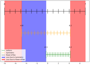
Figure 1: Uniform, Symmetric and Hardware-Friendly Quantizers. Illustration of the loss in quantization bins due to hardware friendly constraints.

3 Method

Given a trained floating point network and a representative dataset $D$ of independent and identically distributed samples, our aim is to quantize the network in post-training with hardware-friendly quantizers, namely that are uniform, symmetric and with power-of-two thresholds. Hardware Friendly Post Training Quantization (HPTQ) is a three-tier method for addressing this goal. HPTQ consists of a pre-processing stage followed by activation quantization and weight quantization (see Fig. 2). In the resulting network, activations are quantized per tensor and weights are quantized per channel.

Figure 2: The HPTQ framework. Dashed lines represent statistical information passing, which include also their updates, dotted lines represent data passing and solid lines represent an updated network.

3.1 Pre-Processing

The pre-processing stage consists of folding batch normalization layers into their preceding convolution layers [10], collecting activation statistics using the representative dataset and finally removing outliers from the collected statistics.

Batch-Normalization Folding.

A common technique to reduce model size and computational complexity is batch-normalization folding [10] (also known as batch-normalization fusing) in which batch-normalization layers are folded into the weights of their preceding convolution layers.

Statistics Collection.

In this stage we infer all of the samples in the representative dataset $D$ and collect activation statistics of each layer. Specifically, for each layer $l$ denote the collection of its activations over $D$ by $F_{l}\left(D\right)$. Based on $F_{l}\left(D\right)$ we collect histograms for each tensor as well as the minimum, maximum and mean values per channel. In the reset of this work we assume that activation tensors $\mathbf{X}\in\mathbf{R}^{h\times w\times c}$ have three dimensions where $h$, $w$ and $c$ are the height, weight and number of channels, respectively.

Outlier Removal.

In this step we filter out outliers in the activation histograms using the z-score approach described in [21]. Specifically, we remove histogram bins for which the absolute z-score value is larger than a predefined threshold. This implies that we restrict the range of each histogram bin to a predefined number of standard deviations from its activation mean value. See Figure 3 for an example. Note that since this step updates the histograms, it applies only to the Threshold Selection step (see Figure 2).

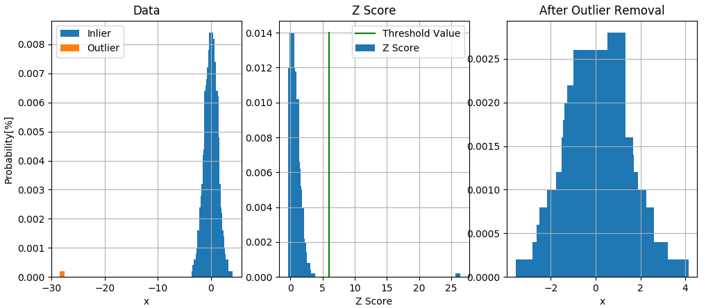
Figure 3: Outlier Removal. Left: an input data distribution. Middle: the respective distribution of absolute z-score values. Right: data distribution after outlier removal.

3.2 Activation Quantization

This stage consists of three steps: threshold selection, shift negative correction (SNC) and activation equalization. In the threshold selection step, we set power-of-two thresholds per tensor. The SNC step is a trick that improves the quantization of signed activation functions with a small negative range [22]. In the activation equalization step we equalize the expected dynamic ranges of activation channels by applying a modified version of a technique that appears in [23].

Threshold Selection.

Given a fixed bit width $n_{b}$, our aim is to find a power-of-two threshold $t$ that minimizes the noise caused by the quantization of each layer $l$ in the network. Formally, for each layer $l$ in the network, our objective is to find a threshold $t$ that minimizes

$$ERR\left(t\right)=\frac{1}{n_{s}}\sum_{X\in F_{l}(D)}d\left(Q(\mathbf{X},t,n_{b}),\mathbf{X}\right),$$ (6)

where $n_{s}$ is the size of the representative dataset, $F_{l}(D)$ is the collection of activation tensors in the $l$-th layer and $d$ is some error measurement.

In an ablation study we examine the effect of several possible quantization error measurements on the actual task accuracy, including $\mathrm{L}_{p}$ Norms [24] and Kullback–Leibler (KL) divergence [25]. Our results show that Mean Square Error (MSE) [24] achieves the best performance (see Table 7). Thus, the objective of the threshold selection is to minimize

$$ERR\left(t\right)=\frac{1}{n_{s}}\sum_{X\in F_{l}(D)}\left(Q(\mathbf{X},t,n_{b})-\mathbf{X}\right)^{2}.$$ (7)

In practice, we approximate a solution to this minimization problem by estimating the noise based on the histogram corresponding to layer $l$ collected in the Statistics Collection step above. The restriction of the threshold to power-of-two values implies that the search space is discrete. Let $M=\max\limits_{\mathbf{X}\in F_{l}(D)}\max\limits_{i,j,k}\left|\mathbf{X}\right|_{i,j,k}$ be the maximal absolute value of an activation in $\mathbf{X}$ over the representative dataset $D$ that was collected in the Statistics Collection step above and define the no-clipping threshold:

$$t_{nc}=2^{\left\lceil\log_{2}M\right\rceil}.$$ (8)

Note that the clipping noise induced by the threshold $t_{nc}$ is zero and that for any power-of-two threshold larger than $t_{nc}$, the noise is increased. Thresholds smaller than $t_{nc}$ may reduce the noise, albeit, at the cost of increasing the clipping noise. Therefore, we search for a threshold minimizing the quantization error starting with $t_{nc}$ and iteratively decreasing it (see. Algorithm 1).

Data: quantization error estimator ERR ; no-clipping threshold $t_{nc}$; bit-width $n_{b}$; $n$ iterations

Result: $t$ threshold value

$e_{min}=\infty$ ;

$t=t_{nc}$ ;

for i in 0 to n do

       $t_{i}=\frac{t_{nc}}{2^{i}}$ ;

       $e_{i}=ERR\left(t_{i},n_{b}\right)$ ;

       if $e_{i}<e_{min}$ then

             $t=t_{i}$ ;

             $e_{min}=e_{i}$

      

return $t$

Algorithm 1 Constraint threshold selection

Shift Negative Correction (SNC).

Recent works have shown benefits in using signed, non-linear activation functions, such as Swish [26], PReLU and HSwish [27]. However, a signed symmetric quantization of these functions can be inefficient due to differences between their negative and positive dynamic ranges. The main idea in SNC is to reduce the quantization noise of an unsigned activation function with a small negative range (relatively to its positive range). This is done by adding a positive constant to the activation values (shifting its values) and using an unsigned quantizer with the same threshold. This effectively doubles the quantization grid resolution. Note that shifting the values can imply added clipping noise on the one hand but reduced rounding noise on the other.

This step can be viewed as an adaptation to PTQ of a technique that appears in [22], where activations are shifted and scaled in order to match a given dynamic range of a quantizer. Here, we do not add scaling due to its implied added complexity. Specifically, let $\phi$ be the activation function in some layer $l$ in the network, let $t$ be its threshold, calculated in the Threshold Selection step above and let $\rm{s}=\min\limits_{\mathbf{X}\in F_{l}(D)}\min\limits_{i,j,k}\mathbf{X}_{i,j,k}$ be its minimal (negative) activation value over the representative dataset $D$, collected in the Statistics Collection step above. If $\frac{|\rm{s}|}{t}<\alpha$ for a hyperparameter $\alpha$, then we replace $\phi$ with a shifted version $\tilde{\phi}=\phi+|s|$ and replace the signed quantizer with an unsigned quantizer followed by another shift operation as follows:

$$Q^{\rm{s}}(\phi(\mathbf{X}),t,n_{b})\xrightarrow{}Q^{\rm{us}}(\tilde{\phi}(\mathbf{X}),t,n_{b})-|s|,$$ (9)

where $Q^{\rm{s}}(\phi(\mathbf{X}),t,n_{b})$ is the signed quantizer, $Q^{\rm{us}}(\tilde{\phi}(\mathbf{X}),t,n_{b})$ is the unsigned quantizer and $n_{b}$ is the bit-width. In practice, the last subtraction of $|\rm{s}|$ is folded into the following operation in the network.

Activation Equalization.

In this step, we equalize activation ranges per channel similarly to the methods presented in [23, 28]. Here, we set the scale-per-channel factor according to the value of the threshold that is selected per-tensor. The motivation to use this scaling factor in order to equalize the activation ranges is to use the maximum range of the quantization bins for each channel (see Figure 4).

The authors in [23, 28] suggest to perform channel equalization by exploiting the positive scale equivariance property of activation functions. It holds for any piece-wise linear activation function in its relaxed form: ${\phi}\left(\bm{S}\bm{x}\right)=\bm{S}\hat{\phi}\left(\bm{x}\right)$ where $\phi$ is a piece-wise linear function, $\hat{\phi}$ is its modified version that fits this requirement and $\bm{S}=diag\left(\bm{s}\right)$ is a diagonal matrix with $\bm{s}_{k}$ denoting the scale factor for channel $k$.

The positive scaling equivariance can be applied on the following set of consecutive layers: a linear operation, a piece-wise linear function $\phi$ and an additional linear operation. This is demonstrated in the following equation:

$$\begin{split}\mathbf{y}&=\mathbf{W}_{2}\phi\left(\mathbf{W}_{1}\mathbf{x}+\bm{b}_{1}\right)+\bm{b}_{2}=\mathbf{W}_{2}\phi\left({\bm{S}}{\bm{S}^{-1}}\left(\mathbf{W}_{1}\mathbf{x}+\bm{b}_{1}\right)\right)+\bm{b}_{2}\\ &=\mathbf{W}_{2}\bm{S}\hat{\phi}({\bm{S}^{-1}}\left(\mathbf{W}_{1}\mathbf{x}+\bm{b}_{1}\right))+\bm{b}_{2},\end{split}$$ (10)

where $\mathbf{W}_{1}$ and $\bm{b}_{1}$ are the first layer’s weights and bias, $\mathbf{W}_{2}$ and $\bm{b}_{2}$ are the second layer’s weights and bias. Although Eq. 10 demonstrates the case of fully-connected layers, it can be also extended for CNNs where the scaling is performed per channel.

We present a use case of channel equalization named Max Channel Equalization which can be applied in any quantization scheme. We assume that $\hat{\phi}$ is one of the following non-linear functions: ReLU, ReLU8 or PReLU. Given the quantization threshold $t$ of a non-linear function as well as the maximal activation value of the $k^{th}$ channel $v_{k}=\max\limits_{\mathbf{X}\in F_{l}(D)}\max\limits_{i,j}|\mathbf{X}_{i,j,k}|$, where $\mathbf{X}$ is the activation tensor of the $l^{th}$ layer, we set:

$$\bm{s}_{k}=\min\left(\frac{v_{k}}{t},1\right),$$ (11)

so that the maximal value of each channel in tensor $\mathbf{X}$ will be the threshold value (see Figure 4).

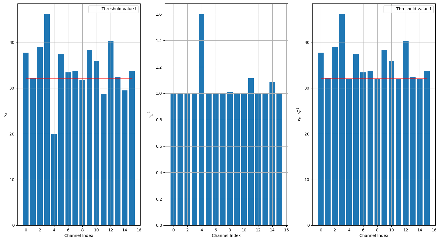
Figure 4: An example of Max Channel Equalization using MobileNetV2 [29] . Left: the max value $\bm{v}_{max}$ of each channel. Middle: the inverse scale factor $\frac{1}{\bm{s}_{k}}$ for each channel $k$. Right: the max value of each channel after equalization using this scaling factor.

3.3 Weight Quantization

In the Weight Quantization stage we quantize the network’s weights. It was shown in [30, 31] that weight quantization with scaling per channel improves accuracy. Moreover, this work presents an efficient dot product and convolution implementation supporting per-channel quantization. Our Weight Quantization stage consists of per-channel threshold selection and bias correction [23].

Threshold Selection.

As noted above, weight quantization is performed per-channel. Its thresholds are selected similarly to activation thresholds (see Algorithm 1). However, a key difference is that here the search is performed directly on the weight values, opposed to the statistical values that are used for activation. More precisely, given the weights $\bm{w}\in\mathbb{R}^{n}$ of some channel in the network, the initial no-clipping threshold is

$$t_{nc}=2^{\left\lceil\log_{2}\left(\max\limits_{i}\left|\bm{w}_{i}\right|\right)\right\rceil},$$ (12)

where $\bm{w}_{i}\in\mathbb{R}$ are the entries of $\bm{w}$. Additionally, the error induced by a threshold $t$ is

$$ERR\left(t\right)=MSE(Q(\bm{w},t,n_{b}),\bm{w})=\frac{1}{n}\sum_{i}\left(Q(\bm{w}_{i},t,n_{b})-\bm{w}_{i}\right)^{2}.$$ (13)

Note that as with activations, MSE is selected as an error measurement since it yields the best performance (see Table 10).

Bias Correction.

Quantization of weights induce bias shifts to activation means that may lead to detrimental behaviour in the following layers [23, 32]. Explicitly, let $\bm{y}=\mathbf{W}\bm{x}+\bm{b}$ be the floating point output of a fully connected layer where $\bm{x},\mathbf{W},\bm{b}$ are the floating-point input activation, weight and bias, respectively. Denote the quantized weights of the layer by $\tilde{\mathbf{W}}=Q(\mathbf{W},t,n_{b})$ and the corresponding output by $\tilde{\bm{y}}=\tilde{\mathbf{W}}\bm{x}+\bm{b}$. The induced bias shift $\mathbb{E}\left[\bm{y}\right]-\mathbb{E}\left[\tilde{\bm{y}}\right]$ can be expressed as follows:

$$\mathbb{E}\left[\bm{y}\right]-\mathbb{E}\left[\tilde{\bm{y}}\right]=\mathbb{E}\left[\mathbf{W}-\tilde{\mathbf{W}}\right]\mathbb{E}\left[\bm{x}\right]=\epsilon\mathbb{E}\left[\bm{x}\right].$$ (14)

Several works propose approaches to correct the quantization induced bias. These include using batch-normalization statistics [23], micro training [32] and applying scale and shift per channel [33].

We adopt the solution in [23], in which the bias shift is fixed by modifying the layer’s bias vector

$$\tilde{\bm{b}}=\bm{b}-\epsilon\mathbb{E}\left[\bm{x}\right],$$ (15)

where $\mathbb{E}\left[\bm{x}\right]$ is the per channel empirical mean obtain in the Statistic Collection stage above. Note that although the above is written for a fully connected layer, it applies to convolutional layers as well, as shown in [23].

4 Experimental Results

In this section we evaluate the performance of HPTQ with 8-bit quantization over different tasks and a variety of network architectures. The experiments are divided into two parts. The first part presents an overall performance comparison to the floating point baseline as well as to state-of-the-art quantization approaches. The second part presents an ablation study that analyzes the influence of each technique in HPTQ separately.

4.1 Overall Performance Evaluation

We evaluate the performance of HPTQ on four different tasks: image classification, object detection, semantic segmentation and pose estimation. For each task, we present a comparison between the performance of models quantized by HPTQ and their floating point baselines. Furthermore, for classification and segmentation we provide a comprehensive performance comparison of HPTQ with both PTQ and QAT state-of-the art quantization methods.

We use the same set of hyper-parameters for all our experiments. Specifically, the number of image samples in the representative dataset $D$ is 500. The z-score threshold in the outlier removal step is $z_{th}=24$. The SNC threshold is $\alpha=0.25$. Last, for both activations and weights, the number of iterations performed in Algorithm 1 in the threshold selection search is set to $n=10$. One should note that fine-tuning the hyper-parameters per network may lead to further improvement. In all of the tables below $\Delta$ is the difference between the performance of the floating point model and the quantized model, PC indicates the use of weights per channel quantization and PoT indicates power-of-two thresholds.

Classification.

We evaluate HPTQ on the ImageNet classification task [34] using MobileNetV1 [2] , MobileNetV2 [29] and ResNet50 [1] architectures. Tables 1, 2 and 3 present comparisons of HPTQ with other quantization methods, both PTQ and QAT, for the three architectures. The results show that HPTQ achieves competitive performance despite the hardware friendly constraints. In the tables below F-Acc is the floating point accuracy and Q-Acc is the accuracy of the quantized model.

Table 1: ImageNet classification [34] with MobileNetV1 [2]

Type	Method	PC	PoT	F-Acc	Q-Acc	$\Delta$
QAT	QT [10]	✗	✗	70.9	70.0	0.9
	TQT [11]	✗	✓	71.1	71.1	0.0
PTQ	SSBD [28]	✗	✗	70.9	69.95	0.95
	Krishnamoorthi [30]	✓	✗	70.9	70.3	0.6
	Wu et al [35]	✓	✗	71.88	70.39	1.49
	Lee et al [36]	✗	✗	69.5	68.84	0.66
	HPTQ (Our)	✓	✓	70.55	70.41	0.14

Table 2: ImageNet classification [34] with MobileNetV2 [29]

Type	Method	PC	PoT	F-Acc	Q-Acc	$\Delta$
QAT	QT [10]	✗	✗	71.9	70.9	1.0
	RVQuant [37]	✗	✗	70.10	70.29	-0.19
	TQT [11]	✗	✓	71.7	71.8	-0.10
PTQ	AdaQuant [38]	✗	✗	73.03	73.03	0.0
	ZeroQ [15]	✗	✗	73.03	72.91	0.12
	SSBD [28]	✗	✗	71.9	71.29	0.61
	Wu et al [35]	✓	✗	71.88	71.14	0.74
	Krishnamoorthi [30]	✓	✗	71.9	69.7	2.2
	Nagel et al [20]	✗	✗	71.72	70.99	0.73
		✓	✗		71.16	0.56
	DFQ [23]	✗	✗	71.72	70.92	0.8
	Lee et al [36]	✗	✗	71.23	69.5	1.73
	HPTQ (Our)	✓	✓	71.812	71.46	0.352

Table 3: ImageNet classification [34] with ResNet50 [1]

Type	Method	PC	PoT	F-Acc	Q-Acc	$\Delta$
QAT	QT [10]	✗	✗	76.4	74.9	1.5
	RVQuant [37]	✗	✗	75.92	75.67	0.25
	HAWQ-V3 [39]	✓	✗	77.72	77.58	0.14
	LSQ [40]	✗	✗	76.9	76.8	0.1
	TQT [11]	✗	✓	76.9	76.5	0.4
	FAQ [41]	✗	✗	75.4	75.4	0.0
PTQ	ZeroQ [15]	✗	✗	77.72	77.67	0.05
	OCS [42]	✗	✗	76.1	75.9	0.2
	SSBD [28]	✗	✗	75.2	74.95	0.25
	He et al [43]	✗	✗	75.3	75.03	0.27
	Wu et al [35]	✓	✗	76.16	76.05	0.11
	Nagel et al [20]	✗	✗	76.07	75.87	0.2
		✓	✗		75.88	0.19
	Krishnamoorthi [30]	✗	✗	75.2	75.00	0.20
		✓	✗		75.1	0.1
	HPTQ (Our)	✓	✓	75.106	75.018	0.088

Semantic Segmentation.

We evaluate HPTQ on Pascal VOC [44] using DeepLab V3 [6] with MobileNetV2 [29] as a backbone. Table 4 shows that HPTQ achieves competitive results compared to other PTQ methods.

Table 4: Semantic segmentation on Pascal VOC [44] using DeepLab V3 with MobileNetV2 [29] as a backbone. F-mIoU is the floating point mean Intersection-over-Union (mIoU) and Q-mIoU is the mIoU of the quantized model.

Type	Method	PC	PoT	F-mIoU	Q-mIoU	$\Delta$
PTQ	DFQ [23]	✗	✗	72.45	72.33	0.12
	Nagel et al [20]	✗	✗	72.94	72.44	0.50
		✓	✗		72.27	0.67
	HPTQ (Our)	✓	✓	75.57	75.38	0.19

Object Detection.

We evaluate HPTQ on COCO [45] using the SSD detector [4] with several backbones. HPTQ achieves similar Mean Average Precision (mAP) to the floating point baseline as demonstrated in Table 5.

Table 5: Object detection results with HPTQ on COCO [45] using MobileNetV2 [29] and ResNet50 [1] as backbones. F-mAP is the floating point mAP and Q-mAP is the mAP of the quantized model.

Model	F-mAP	Q-mAP
SSD MobileNetV2 [29] 320x320	20.2	20.21
SSD MobileNetV2 [29] FPN Lite 320x320	22.2	21.93
SSD ResNet50 [1] V1 FPN 640x640	34.3	34.3

Pose-Estimation.

We evaluate HPTQ on the single-person pose estimation task using LPN network [7] on the LIP (Look into Person) dataset [46]. We use the PCKh metric [46] for evaluation, which is the head-normalized probability of correct keypoints. HPTQ achieves similar performance to the floating point baseline with only a slight degradation from 81.65 to 81.53 PCKh.

4.2 Ablation Study

We provide an ablation study of HPTQ’s performance on the ImageNet classification task [34] using eleven networks. The study is divided into two parts analyzing activation quantization and weight quantization.

Table 6 compares the performance of HPTQ between four cases: full floating-point, activation quantization, weight quantization and joint quantization of both. The comparison shows that activation quantization causes a larger degradation in performance compared to weight quantization, especially for EfficientNet with Swish activations functions. This might be due to the fact that activation equalization is not applied for these activations.

Table 6: ImageNet classification [34] accuracy with HPTQ in four cases: full floating-point, activation quantization, weight quantization and both activation and weight quantization.

Network	F-Acc	Q-Acc (Activation)	Q-Acc (Weights)	Q-Acc (Both)
MobileNetV1 [2]	70.558	70.48	70.394	70.418
MobileNetV2 [29]	71.812	71.616	71.668	71.46
NasnetMobile [47]	74.376	74.068	74.352	73.888
VGG16 [48]	70.956	70.834	70.946	70.81
InceptionV3 [49]	77.908	77.872	77.844	77.85
InceptionResNetV2 [50]	80.284	80.154	80.32	80.14
ResNet50 [1]	75.106	75.072	75.06	75.018
EfficientNet-B0 [51]	77.2	74.3	77.012	74.216
EfficientNet-B0 ReLU${}^{\ref{foot:eff}}$	77.65	77.1	77.568	77.092
DenseNet-121 [52]	74.848	73.252	74.784	73.356
Xception [53]	79.05	79.048	79.062	78.972

Activation Quantization Analysis.

In this analysis we evaluate the influence of the different methods used for quantizing the activations (without quantizing the weights). The analysis is performed with eleven different network architectures on the ImageNet classification [34] task. Table 7 shows an accuracy comparison using four different threshold selection methods without applying any other of the activation quantization steps. NC indicates using the no-clipping threshold. Mean Square Error (MSE), Mean Average Error (MAE) and Kullback–Leibler (KL) are three different error measurements $d$ in Equation 6.

Table 7: ImageNet classification [34] accuracy with activations quantized using different threshold selection methods (weights are in floating point).

Network	NC	MSE	MAE	KL
MobileNetV1 [2]	70.406	70.434	60.218	70.418
MobileNetV2 [29]	71.25	71.458	65.918	71.482
VGG16 [48]	70.8	70.764	58.37	65.096
ResNet50 [1]	74.612	74.996	67.896	59.556

Table 8 shows the incremental accuracy influence on ImageNet classification [34] of the methods used by HPTQ for activation quantization (without quantizing weights). Note that SNC is applied in all of the experiments in the table and its influence is studied separately below. The table shows that all of the methods result in an improvement. Note that fine-tuning the z-score threshold $z_{th}$ per network may lead to further improvement.

Table 8: The accuracy influence of the different activation quantization methods used by HPTQ for ImageNet classification [34] when keeping all weights in floating point. Baseline is quantization with no-clipping thresholds, +Eq. means adding max channel equalization, +MSE Th. means replacing the no-clipping thresholds with MSE and +z-score means applying z-score outlier removal.

Network Name	Baseline	+Eq.	+MSE Th.	+z-score
MobileNetV1 [2]	70.406	70.418	70.48	70.48
MobileNetV2 [29]	71.25	71.34	71.528	71.616
NasnetMobile [47]	18.572	18.484	73.486	74.068
VGG16 [48]	70.8	70.696	70.888	70.834
InceptionV3 [49]	77.658	77.646	77.832	77.872
InceptionResNetV2 [50]	49.132	49.238	80.014	80.154
ResNet50 [1]	74.612	74.654	75.086	75.072
EfficientNet-B0 [51]	13.562	13.736	74.096	74.3
EfficientNet-B0 ReLU${}^{\ref{foot:eff}}$	74.298	76.298	76.956	77.1
DenseNet-121 [52]	56.08	55.916	73.28	73.252
Xception [53]	48.718	48.784	78.87	79.048

Table 9 shows the accuracy improvement achieved by applying Shift Negative Correction (SNC). Specifically, the table compares the performance of several versions of MobileNetV1, each with different non-linear functions, with a full flow of activation quantization.

Table 9: ImageNet classification accuracy [34] using HPTQ with and without SNC of MobileNetV1 [2] trained with different non-linear functions.

	Swish	Leaky ReLU ($\alpha=0.1$)	PReLU	SELU
Float	73.522	72.866	73.114	72.032
Without SNC	60.98	71.966	72.548	69.726
With SNC	71.146	72.588	72.548	70.902

Weight Quantization Analysis.

In this analysis we evaluate the influence of the different methods used for quantizing weights (without quantizing activations). The analysis is performed with eleven different network architectures on the ImageNet classification [34] task.

Table 10 shows an accuracy comparison of each quantized network using four different threshold selection methods (without applying bias correction). NC indicates using the no-clipping threshold. Mean Square Error (MSE), Mean Average Error (MAE) and Kullback–Leibler (KL) are three different error measurements $d$ in Equation 6. Similarly to the results for activation quantization in Table 7, the MSE error measurement achieves the best results.

Table 10: ImageNet classification [34] accuracy with weights quantized using different threshold selection methods (activations are in floating point).

Network	NC	MSE	MAE	KL
MobileNetV1 [2]	68.75	68.756	64.242	64.968
MobileNetV2 [29]	69.562	69.758	67.57	62.394
NasnetMobile [47]	74.188	74.232	72.79	73.358
VGG16 [48]	70.944	70.94	67.486	70.472
InceptionV3 [49]	77.768	77.82	70.91	74.28
InceptionResNetV2 [50]	80.244	80.276	78.676	77.112
ResNet50 [1]	75.068	75.11	72.352	73.418
EfficientNet-B0 [51]	76.822	76.822	75.86	75.554
EfficientNet-B0 ReLU${}^{\ref{foot:eff}}$	77.078	77.218	76.916	76.674
DenseNet-121 [52]	74.734	74.736	72.102	60.17
Xception [53]	79.006	79.006	77.47	75.374

Table 11 shows the incremental accuracy influence of the two methods (per channel quantization and bias correction) used in HPTQ for weight quantization (without quantizing activations) on the ImageNet classification task [34]. This table shows that both of our methods result in improvement.

Table 11: The incremental influence of applying per-channel threshold selection (Per ch.) and bias correction (Bias corr.) on ImageNet [34] classification accuracy. Baseline means quantization with MSE threshold applied per tensor.

Network	Baseline	Per ch.	+Bias corr.
MobileNetV1 [2]	0.966	68.756	70.394
MobileNetV2 [29]	0.398	69.758	71.668
NasnetMobile [47]	73.494	74.232	74.352
VGG16 [48]	70.814	70.94	70.946
InceptionV3 [49]	76.42	77.82	77.844
InceptionResNetV2 [50]	80.066	80.276	80.32
ResNet50 [1]	74.718	75.11	75.06
EfficientNet-B0 [51]	2.524	76.822	77.012
EfficientNet-B0 ReLU${}^{\ref{foot:eff}}$	0.682	77.218	77.568
DenseNet-121 [52]	72.986	74.736	74.784
Xception [53]	78.786	79.006	79.062

5 Conclusions

In this work we propose HPTQ, a method for hardware-friendly post-training quantization. HPTQ offers a flow that adapts and synergistically combines several known quantization techniques both for weights and activations. We extensively evaluated the performance of HPTQ on four tasks: classification, object detection, semantic segmentation and pose estimation. Notably, for all of the tasks we demonstrated that competitive results can be obtained under our hardware-friendly constraints of uniform and symmetric quantization with power-of-two thresholds. In addition, we performed an ablation study in which we presented the contributions of each of the methods used by HPTQ.

References

- [1] Kaiming He, Xiangyu Zhang, Shaoqing Ren, and Jian Sun. Deep residual learning for image recognition. In Proceedings of the IEEE conference on computer vision and pattern recognition, pages 770–778, 2016.
- [2] Andrew G Howard, Menglong Zhu, Bo Chen, Dmitry Kalenichenko, Weijun Wang, Tobias Weyand, Marco Andreetto, and Hartwig Adam. Mobilenets: Efficient convolutional neural networks for mobile vision applications. arXiv preprint arXiv:1704.04861, 2017.
- [3] Shaoqing Ren, Kaiming He, Ross Girshick, and Jian Sun. Faster r-cnn: Towards real-time object detection with region proposal networks. arXiv preprint arXiv:1506.01497, 2015.
- [4] Wei Liu, Dragomir Anguelov, Dumitru Erhan, Christian Szegedy, Scott Reed, Cheng-Yang Fu, and Alexander C Berg. Ssd: Single shot multibox detector. In European conference on computer vision, pages 21–37. Springer, 2016.
- [5] Tsung-Yi Lin, Piotr Dollár, Ross Girshick, Kaiming He, Bharath Hariharan, and Serge Belongie. Feature pyramid networks for object detection. In Proceedings of the IEEE conference on computer vision and pattern recognition, pages 2117–2125, 2017.
- [6] Liang-Chieh Chen, George Papandreou, Florian Schroff, and Hartwig Adam. Rethinking atrous convolution for semantic image segmentation. arXiv preprint arXiv:1706.05587, 2017.
- [7] Zhe Zhang, Jie Tang, and Gangshan Wu. Simple and lightweight human pose estimation. arXiv preprint arXiv:1911.10346, 2019.
- [8] Zhe Cao, Gines Hidalgo, Tomas Simon, Shih-En Wei, and Yaser Sheikh. Openpose: realtime multi-person 2d pose estimation using part affinity fields. IEEE transactions on pattern analysis and machine intelligence, 43(1):172–186, 2019.
- [9] Amir Gholami, Sehoon Kim, Zhen Dong, Zhewei Yao, Michael W Mahoney, and Kurt Keutzer. A survey of quantization methods for efficient neural network inference. arXiv preprint arXiv:2103.13630, 2021.
- [10] Benoit Jacob, Skirmantas Kligys, Bo Chen, Menglong Zhu, Matthew Tang, Andrew Howard, Hartwig Adam, and Dmitry Kalenichenko. Quantization and training of neural networks for efficient integer-arithmetic-only inference. In Proceedings of the IEEE Conference on Computer Vision and Pattern Recognition, pages 2704–2713, 2018.
- [11] Sambhav R Jain, Albert Gural, Michael Wu, and Chris H Dick. Trained quantization thresholds for accurate and efficient fixed-point inference of deep neural networks. arXiv preprint arXiv:1903.08066, 2019.
- [12] Jungwook Choi, Zhuo Wang, Swagath Venkataramani, Pierce I-Jen Chuang, Vijayalakshmi Srinivasan, and Kailash Gopalakrishnan. Pact: Parameterized clipping activation for quantized neural networks. arXiv preprint arXiv:1805.06085, 2018.
- [13] Ruihao Gong, Xianglong Liu, Shenghu Jiang, Tianxiang Li, Peng Hu, Jiazhen Lin, Fengwei Yu, and Junjie Yan. Differentiable soft quantization: Bridging full-precision and low-bit neural networks. In Proceedings of the IEEE/CVF International Conference on Computer Vision, pages 4852–4861, 2019.
- [14] Ron Banner, Yury Nahshan, Elad Hoffer, and Daniel Soudry. Post-training 4-bit quantization of convolution networks for rapid-deployment. arXiv preprint arXiv:1810.05723, 2018.
- [15] Yaohui Cai, Zhewei Yao, Zhen Dong, Amir Gholami, Michael W Mahoney, and Kurt Keutzer. Zeroq: A novel zero shot quantization framework. In Proceedings of the IEEE/CVF Conference on Computer Vision and Pattern Recognition, pages 13169–13178, 2020.
- [16] Markus Nagel, Rana Ali Amjad, Mart Van Baalen, Christos Louizos, and Tijmen Blankevoort. Up or down? adaptive rounding for post-training quantization. In International Conference on Machine Learning, pages 7197–7206. PMLR, 2020.
- [17] Jun Fang, Ali Shafiee, Hamzah Abdel-Aziz, David Thorsley, Georgios Georgiadis, and Joseph H Hassoun. Post-training piecewise linear quantization for deep neural networks. In European Conference on Computer Vision, pages 69–86. Springer, 2020.
- [18] Hai Victor Habi, Roy H. Jennings, and Arnon Netzer. Hmq: Hardware friendly mixed precision quantization block for cnns. In Andrea Vedaldi, Horst Bischof, Thomas Brox, and Jan-Michael Frahm, editors, Computer Vision – ECCV 2020, pages 448–463, Cham, 2020. Springer International Publishing.
- [19] Stefan Uhlich, Lukas Mauch, Fabien Cardinaux, Kazuki Yoshiyama, Javier Alonso Garcia, Stephen Tiedemann, Thomas Kemp, and Akira Nakamura. Mixed precision dnns: All you need is a good parametrization. arXiv preprint arXiv:1905.11452, 2019.
- [20] Markus Nagel, Marios Fournarakis, Rana Ali Amjad, Yelysei Bondarenko, Mart van Baalen, and Tijmen Blankevoort. A white paper on neural network quantization. arXiv preprint arXiv:2106.08295, 2021.
- [21] Charu C Aggarwal. Outlier analysis. In Data mining, pages 237–263. Springer, 2015.
- [22] Yash Bhalgat, Jinwon Lee, Markus Nagel, Tijmen Blankevoort, and Nojun Kwak. Lsq+: Improving low-bit quantization through learnable offsets and better initialization. In Proceedings of the IEEE/CVF Conference on Computer Vision and Pattern Recognition Workshops, pages 696–697, 2020.
- [23] Markus Nagel, Mart van Baalen, Tijmen Blankevoort, and Max Welling. Data-free quantization through weight equalization and bias correction. In Proceedings of the IEEE International Conference on Computer Vision, pages 1325–1334, 2019.
- [24] Yury Nahshan, Brian Chmiel, Chaim Baskin, Evgenii Zheltonozhskii, Ron Banner, Alex M Bronstein, and Avi Mendelson. Loss aware post-training quantization. arXiv preprint arXiv:1911.07190, 2019.
- [25] Szymon Migacz. 8-bit inference with tensorrt. 2017.
- [26] Prajit Ramachandran, Barret Zoph, and Quoc V Le. Searching for activation functions. arXiv preprint arXiv:1710.05941, 2017.
- [27] Andrew Howard, Mark Sandler, Grace Chu, Liang-Chieh Chen, Bo Chen, Mingxing Tan, Weijun Wang, Yukun Zhu, Ruoming Pang, Vijay Vasudevan, et al. Searching for mobilenetv3. In Proceedings of the IEEE International Conference on Computer Vision, pages 1314–1324, 2019.
- [28] Eldad Meller, Alexander Finkelstein, Uri Almog, and Mark Grobman. Same, same but different-recovering neural network quantization error through weight factorization. arXiv preprint arXiv:1902.01917, 2019.
- [29] Mark Sandler, Andrew Howard, Menglong Zhu, Andrey Zhmoginov, and Liang-Chieh Chen. Mobilenetv2: Inverted residuals and linear bottlenecks. In Proceedings of the IEEE conference on computer vision and pattern recognition, pages 4510–4520, 2018.
- [30] Raghuraman Krishnamoorthi. Quantizing deep convolutional networks for efficient inference: A whitepaper. arXiv preprint arXiv:1806.08342, 2018.
- [31] Mohammad Rastegari, Vicente Ordonez, Joseph Redmon, and Ali Farhadi. Xnor-net: Imagenet classification using binary convolutional neural networks. In European conference on computer vision, pages 525–542. Springer, 2016.
- [32] Alexander Finkelstein, Uri Almog, and Mark Grobman. Fighting quantization bias with bias. arXiv preprint arXiv:1906.03193, 2019.
- [33] Ron Banner, Yury Nahshan, and Daniel Soudry. Post training 4-bit quantization of convolutional networks for rapid-deployment. In Advances in Neural Information Processing Systems, volume 32, pages 7950–7958. Curran Associates, Inc., 2019.
- [34] Jia Deng, Wei Dong, Richard Socher, Li-Jia Li, Kai Li, and Li Fei-Fei. Imagenet: A large-scale hierarchical image database. In 2009 IEEE conference on computer vision and pattern recognition, pages 248–255. Ieee, 2009.
- [35] Hao Wu, Patrick Judd, Xiaojie Zhang, Mikhail Isaev, and Paulius Micikevicius. Integer quantization for deep learning inference: Principles and empirical evaluation. arXiv preprint arXiv:2004.09602, 2020.
- [36] Jun Haeng Lee, Sangwon Ha, Saerom Choi, Won-Jo Lee, and Seungwon Lee. Quantization for rapid deployment of deep neural networks. arXiv preprint arXiv:1810.05488, 2018.
- [37] Eunhyeok Park, Sungjoo Yoo, and Peter Vajda. Value-aware quantization for training and inference of neural networks. In Proceedings of the European Conference on Computer Vision (ECCV), pages 580–595, 2018.
- [38] Itay Hubara, Yury Nahshan, Yair Hanani, Ron Banner, and Daniel Soudry. Improving post training neural quantization: Layer-wise calibration and integer programming. arXiv preprint arXiv:2006.10518, 2020.
- [39] Zhewei Yao, Zhen Dong, Zhangcheng Zheng, Amir Gholami, Jiali Yu, Eric Tan, Leyuan Wang, Qijing Huang, Yida Wang, Michael Mahoney, et al. Hawq-v3: Dyadic neural network quantization. In International Conference on Machine Learning, pages 11875–11886. PMLR, 2021.
- [40] Steven K Esser, Jeffrey L McKinstry, Deepika Bablani, Rathinakumar Appuswamy, and Dharmendra S Modha. Learned step size quantization. arXiv preprint arXiv:1902.08153, 2019.
- [41] Jeffrey L McKinstry, Steven K Esser, Rathinakumar Appuswamy, Deepika Bablani, John V Arthur, Izzet B Yildiz, and Dharmendra S Modha. Discovering low-precision networks close to full-precision networks for efficient inference. In 2019 Fifth Workshop on Energy Efficient Machine Learning and Cognitive Computing-NeurIPS Edition (EMC2-NIPS), pages 6–9. IEEE, 2019.
- [42] Ritchie Zhao, Yuwei Hu, Jordan Dotzel, Chris De Sa, and Zhiru Zhang. Improving neural network quantization without retraining using outlier channel splitting. In International conference on machine learning, pages 7543–7552. PMLR, 2019.
- [43] Xiangyu He and Jian Cheng. Learning compression from limited unlabeled data. In Proceedings of the European Conference on Computer Vision (ECCV), pages 752–769, 2018.
- [44] Mark Everingham, Luc Van Gool, Christopher KI Williams, John Winn, and Andrew Zisserman. The pascal visual object classes (voc) challenge. International journal of computer vision, 88(2):303–338, 2010.
- [45] Tsung-Yi Lin, Michael Maire, Serge Belongie, James Hays, Pietro Perona, Deva Ramanan, Piotr Dollár, and C Lawrence Zitnick. Microsoft coco: Common objects in context. In European conference on computer vision, pages 740–755. Springer, 2014.
- [46] Xiaodan Liang, Ke Gong, Xiaohui Shen, and Liang Lin. Look into person: Joint body parsing & pose estimation network and a new benchmark. IEEE transactions on pattern analysis and machine intelligence, 41(4):871–885, 2018.
- [47] Barret Zoph, Vijay Vasudevan, Jonathon Shlens, and Quoc V Le. Learning transferable architectures for scalable image recognition. In Proceedings of the IEEE conference on computer vision and pattern recognition, pages 8697–8710, 2018.
- [48] Karen Simonyan and Andrew Zisserman. Very deep convolutional networks for large-scale image recognition. arXiv preprint arXiv:1409.1556, 2014.
- [49] Christian Szegedy, Vincent Vanhoucke, Sergey Ioffe, Jon Shlens, and Zbigniew Wojna. Rethinking the inception architecture for computer vision. In Proceedings of the IEEE conference on computer vision and pattern recognition, pages 2818–2826, 2016.
- [50] Christian Szegedy, Sergey Ioffe, Vincent Vanhoucke, and Alexander Alemi. Inception-v4, inception-resnet and the impact of residual connections on learning. In Proceedings of the AAAI Conference on Artificial Intelligence, volume 31, 2017.
- [51] Mingxing Tan and Quoc Le. Efficientnet: Rethinking model scaling for convolutional neural networks. In International Conference on Machine Learning, pages 6105–6114. PMLR, 2019.
- [52] Gao Huang, Zhuang Liu, Laurens Van Der Maaten, and Kilian Q Weinberger. Densely connected convolutional networks. In Proceedings of the IEEE conference on computer vision and pattern recognition, pages 4700–4708, 2017.
- [53] François Chollet. Xception: Deep learning with depthwise separable convolutions. In Proceedings of the IEEE conference on computer vision and pattern recognition, pages 1251–1258, 2017.