Central configurations on the plane with $N$ heavy and $k$ light bodies

Abstract

We study the problem of planar central configurations with $N$ heavy bodies and $k$ bodies with arbitrary small masses. We derive the equation which describe the limit of light masses going to zero, which can be seen as the equation for central configurations in the anisotropic plane. Using computer rigorous computations we compute all central configurations for $N=2$ and $k=3,4$ and for the derived limit problem. We show that the results are consistent.

1 Introduction

The main problem of the classical celestial mechanics is the $n$-body problem, i.e. the description of the motion of $n$ point masses under their mutual Newtonian gravitational forces. This problem is entirely solved for $n=2$, while for $n\geq 2$ only partial results exist.

A central configuration, denoted here as CC, is an initial configuration, such that if the particles were all released with zero velocity, they would collapse toward the center of mass at the same time. In the planar case, CCs are initial positions for periodic solutions of the $n$-body problem where bodies move on a Keplerian elliptical orbits preserving the shape of the configuration. The circular orbits give rise to solutions for which the configuration rotates at constant angular speed. This is called a relative equilibrium solution (see Figure 1). The other orbits give rise to solutions where radius and the angular speed are not constant.

Figure 1: If we give the particles an appropriate angular velocity such that gravitational forces $F_{i}$ balance (equilibrate) centrifugal forces $R_{i}$, they will move along circular orbits.

1.1 The state of the art

It is conjectured in [W41] that there are finitely many isometry classes of CCs. The conjecture appears as the sixth problem of Smale’s eighteen problems for the 21st century [Sm98]. We refer to this problem in short as CC finiteness. From among abundant literature on the subject, let us mention two important works [HM05] and [AK12] which aim at studying the problem in the most general setting and provide results for $n=4$ and $n=5$ with (almost) arbitrary masses. In [HM05] the authors give a computer assisted proof of CC finiteness for $n=4$ for any system of positive masses; in [AK12] the problem for $n=4$ is proven without computer assistance and the finiteness for $n=5$ is proven for arbitrary positive masses with the possible exception of those CCs where quintuples of positive masses belongs to a given codimension 2 subvariety of the mass space. It is interesting to note that when masses are equal, there are finitely many isometry classes of CCs and this case belongs to the aforementioned subvariety (see [MZ19]). A common feature of these works is that they give a quite poor estimate for the maximum number of CCs. In this context it is worth to mention the work of Simo, based on extensive numerical studies. In [Si78] he gives the number of CCs for all possible masses for $n=4$.

The papers [AK12, HM05, Moe01, HJ11] which are concerned with CC finiteness for all masses study the polynomial equations derived from the equations for CC using the algebraic geometry tools. The approach we pursue is different as we study the equations for CCs using rigorous numerics. While our results published so far (see [MZ19, MZ20]) refer to the equal masses case, our program allows to process boxes in the mass space, hence in principle we can cover the whole mass space and find the number of CCs with all masses. However, there are several obstacles in the case of different masses: some of the masses approaching zero and possible bifurcations. In the current paper, we try to overcome the former problem.

1.2 Our contribution

We look for CCs in the situation when the massess of certain bodies approach zero as the positions of these bodies move closer together (approaching the same point). We derive equations for this limit problem, which can be seen as the equations for central configurations in the anisotropic plane. Our results can be seen as a generalization of the results by Xia [X91], where the case of two light bodies was considered. We perform computer assisted proofs of full listings of CCs in the anisotropic plane for $k=3,4$. The anisotropy parameters correspond to CCs for two heavy bodies with equal masses and $k$ light bodies with very small equal masses in the neighborhood of Lagrange point $L_{4}$ of the restricted two body problem. We also perform rigorous computations of all CCs for $(2+k)$-body problem in the corresponding region of configuration space. The results of both computations are in very good agreement.

The content of the paper is as follows. In Section 2 we recall equations for central configurations. In Section 3 we derive the reduced set of equations for CCs where we remove the rotational symmetry and the system of equations becomes amenable to a direct application of the implicit function theorem. In Section 4 the limit of vanishing masses is studied, the limit problem is derived and basic theorem about the continuation of solutions of the limit problem is proved. In Section 5 we study general properties of the limit problem and we establish some a priori bounds. In Section 6 we find analytically several solutions of the limit problem. In Section 7 we present computer assisted proofs for the limit problem with $k=3,4$ and corresponding CCs for $(2+k)$-bodies with $k=3,4$.

Proofs which are either very simple, or analogous to those in [MZ19] are contained in Appendix A.

1.3 Notation

Throughout the paper we use the following notation:

• body — point characterized by its position $q\in\mathbb{R}^{2}$ and the mass $m$;

• CC – central configuration

• CC_n – central configuration of $n$ point masses (bodies); $q\in\mbox{CC${}_{n}$}$ — $q=(q_{1},\ldots,q_{n})$ is a central configuration of $n$ bodies;

• $r_{ij}=|q_{i}-q_{j}|$, where $q_{i},q_{j}$ are positions of bodies.

Usually we use letters $p$ and $q$ for light and heavy bodies, respectively. Uppercase $P$ and $Q$ denote their respective configurations, with subscripts and superscripts indicating the number of bodies and vector of masses. Both these parameters are consider constant when solving the equations for central configurations (see equation (1)).

• $Q_{N}^{m}$ and $P_{k}^{\mu}$, where

  • $(q_{1},\ldots,q_{N})$ — configuration of heavy bodies with masses $m_{1},\ldots,m_{N}$, respectively; we use $m=(m_{i})_{i=1,\ldots,N}$

  • $(p_{1},\ldots,p_{k})$ — configuration of light bodies with masses $\mu_{1},\ldots,\mu_{k}$, respectively; use $\mu=(\mu_{i})_{i=1,\ldots,k}$

  • $x\in{\rm RE}(Q_{N})$ — $x$ is a relative normalized CC in the restricted $(N+1)$-body problem for the configuration $Q_{N}$ (see Definition 3);

  • $\mbox{CC$$}(W,Q_{N}^{m},x,\mu)$ — central configuration of potential $W$ induced by $(Q_{N},x)$ for $\mu$ (see Definition 4).

  If we indicate masses explicitly we sometimes omit superscripts and just we write $Q_{N}$ or $P_{k}$.

When we focus only on light bodies we use:

• rbp${}{(k,a,b)}$ – CC of restricted $k$ light body problem (see Definition5), solutions of the anisotropic central configuration problem (71).

2 Central configurations

Assume there are a group $Q_{N}^{m}\in\left(\mathbb{R}^{2}\right)^{N}$ of $N$ celestial bodies interacting with each other gravitationally (i.e. due to inverse square Law of Gravitation; gravitational constant is normalized $G=1$). The central configuration problem is to find positions of bodies satisfying the following system of equations

$$\lambda m_{i}(q_{i}-c)=\sum_{\begin{subarray}{c}j=1\\ j\neq i\end{subarray}}^{N}\frac{m_{i}m_{j}}{r_{ij}^{3}}(q_{i}-q_{j})=:f_{i}(q_{1},\dots,q_{n}),\quad i=1,\dots,n,$$ (1)

where $c$ is a center of mass of the configuration and $\lambda\in\mathbb{R}_{+}$ is a scaling factor. It is well-known (see for example [Moe14, MZ19, AK12]) that in equations (1) we can set $c=0$ obtaining

$$-\lambda m_{i}q_{i}=\sum_{j\neq i}\frac{m_{i}m_{j}}{|q_{i}-q_{j}|^{3}}(q_{j}-q_{i})=\frac{\partial U_{N}}{\partial q_{i}},\quad i=1,2,\dots,N$$ (2)

where

$$U_{N}=\sum_{1\leq i<j\leq N}\frac{m_{i}m_{j}}{|q_{i}-q_{j}|}.$$

Definition 1.

[AK12, MZ19] A normalized central configuration $Q_{N}\in\left(\mathbb{R}^{2}\right)^{N}$ is a central configuration with $\lambda=1$ and $c=0$.

From now on we focus on normalized central configurations.

We can reformulate equations (2) with $\lambda=1$ as the problem of finding critical points for certain potential function. Let us define potential

$$V(q_{1},\dots,q_{N})=\sum_{i=1}^{N}\frac{m_{i}q_{i}^{2}}{2}+U_{N}(q_{1},\dots,q_{N})=\sum_{i=1}^{N}\frac{m_{i}q_{i}^{2}}{2}+\sum_{1\leq i<j\leq N}\frac{m_{i}m_{j}}{|q_{i}-q_{j}|}.$$ (3)

Note that for $\lambda=1$ the equations (2) become

$$\frac{\partial V}{\partial q_{i}}(q_{1},\dots,q_{N})=0,\quad i=1,\dots,N.$$ (4)

3 The reduced system of equations for CC

The goal of this section is to derive a set of equations (the reduced system of equations), which gives all (equivalence classes of) CCs and which no longer has $\mathcal{SO}(d)$-symmetry, where $d$ is the dimension of the space. In our case $d=2$ that means that we eliminate rotations around the origin. This section is an extension of the results of Section 5 in [MZ19] and Section 3 in [MZ20].

For the future use we introduce the function $F:\Pi_{i=1}^{n}\mathbb{R}^{d}\to\Pi_{i=1}^{n}\mathbb{R}^{d}$ given by

$$F_{i}(q_{1},\dots,q_{n})=q_{i}-\sum_{j,j\neq i}\frac{m_{j}}{r_{ij}^{3}}(q_{i}-q_{j}),\quad i=1,\dots,n.$$ (5)

Then the system for normalized central configurations

$$q_{i}=\sum_{j,j\neq i}\frac{m_{j}}{r_{ij}^{3}}(q_{i}-q_{j})=:\frac{1}{m_{i}}f_{i}(q_{1},\dots,q_{n}),\quad i=1,\dots,n.$$ (6)

becomes

$$F(q_{1},\dots,q_{n})=0.$$ (7)

It is well known (see [MZ19] and the literature given there) that for any $(q_{1},\ldots,q_{n})\in(\mathbb{R}^{d})^{n}$ holds

$$\sum_{i=1}^{n}f_{i} = 0,$$ (8)

$$\sum_{i=1}^{n}f_{i}\wedge q_{i} = 0,$$ (9)

where $v\wedge w$ is the exterior product of vectors, the result being an element of exterior algebra. If $d=2$ or 3 it can be interpreted as the vector product of $v$ and $w$ in dimension $3$. The identities (8) and (9) are easy consequences of the third Newton’s law (the action equals reaction) and the requirement that the mutual forces between bodies are in direction of the other body.

Consider system (6). After multiplication of $i$-th equation by $m_{i}$ and addition of all equations using (8) we obtain (or rather recover) the center of mass equation

$$\left(\sum_{i=1}^{n}m_{i}\right)c=\sum_{i}m_{i}q_{i}=0.$$ (10)

We can take the equations for $n$-th body and replace it with (10) to obtain an equivalent system

$$q_{i} =\sum_{j,j\neq i}\frac{m_{j}}{r_{ij}^{3}}(q_{i}-q_{j}),\quad i=1,\dots,n-1,$$ (11a)

$$q_{n} =-\frac{1}{m_{n}}\sum_{i=1}^{n-1}m_{i}q_{i}.$$ (11b)

3.1 Non-degenerate solutions of full and reduced systems

Following Moeckel [Moe14] we state the following definition for any $d$, but we are interested in $d=2$, here.

Definition 2.

We say that a normalized central configuration $q=(q_{1},\dots,q_{n})$ is non-degenerate if the rank of $D\!F(q)$ is equal to $dn-\dim\mathcal{SO}(d)$. Otherwise the configuration is called degenerate.

The idea of the above notion of degeneracy is to allow only for the degeneracy related to the rotational symmetry of the problem, because by setting $\lambda=1$ in (1) and keeping the masses fixed we removed the scaling symmetry.

3.1.1 The center of mass reduction

We write the system (11) obtained from (7) after removing the $n$-th body using the center of mass equation (condition (10)) as

$$F_{\mathrm{red}}(q_{1},\dots,q_{n-1})=0,$$ (12)

where $F_{\mathrm{red}}:\Pi_{i=1}^{n-1}\mathbb{R}^{d}\to\Pi_{i=1}^{n-1}\mathbb{R}^{d}$. To be precise we have

$$F_{\mathrm{red},i}(q_{1},\dots,q_{n-1}) = F_{i}(q_{1},\dots,q_{n-1},q_{n}(q_{1},\dots,q_{n-1})),\quad i=1,\dots,n-1$$

where

$$q_{n}(q_{1},\dots,q_{n-1})=-\frac{1}{m_{n}}\sum_{i=1}^{n-1}m_{i}q_{i}.$$ (13)

Lemma 1.

If $q=(q_{1},\dots,q_{n-1},q_{n})$ is a normalized CC. Then

$$\,{\rm rank}\left(D\!F_{\mathrm{red}}(q_{1},\dots,q_{n-1})\right)=\,{\rm rank}\left(D\!F(q_{1},\dots,q_{n-1},q_{n})\right)-d.$$ (14)

An easy proof is left to reader.

For any configuration $q$ we set

$$R_{i}(q_{1},\dots,q_{n})=m_{i}q_{i}-f_{i}(q_{1},\dots,q_{n}),\quad i=1,\dots,n.$$ (15)

With the above notation the system (7) becomes

$$R(q_{1},\dots,q_{n})=(R_{1}(q_{1},\dots,q_{n}),\dots,R_{n}(q_{1},\dots,q_{n}))=0.$$ (16)

For any $(q_{1},\dots,q_{n-1})\in(\mathbb{R}^{2})^{n-1}$ we define

$$\tilde{R}_{i}(q_{1},\dots,q_{n-1})=R_{i}(q_{1},\dots,q_{n-1},q_{n}(q_{1},\dots,q_{n-1})),\quad i=1,\dots,n.$$ (17)

Obviously $\,{\rm rank}(D\tilde{R})(q)=\,{\rm rank}(DF_{\mathrm{red}})(q)$. Observe that for any $(q_{1},\dots,q_{n-1})\in(\mathbb{R}^{d})^{n-1}$ holds

$$\tilde{R}_{n}(q_{1},\dots,q_{n-1})=-\sum_{i=1}^{n-1}\tilde{R}_{i}(q_{1},\dots,q_{n-1}).$$ (18)

Indeed, by (6) we have

$$\sum_{i=1}^{n-1}f_{i}(q_{1},\ldots,q_{n-1},q_{n}(q_{1},\dots,q_{n-1})) = \sum_{i=1}^{n-1}m_{i}q_{i}$$

and by (13)

$$q_{n}(q_{1},\ldots,q_{n-1},q_{n}(q_{1},\dots,q_{n-1})) = -\frac{1}{m_{n}}\sum_{i=1}^{n-1}m_{i}q_{i}$$

$$= -\frac{1}{m_{n}}\sum_{i=1}^{n-1}f_{i}(q_{1},\ldots,q_{n-1},q_{n}(q_{1},\dots,q_{n-1}))$$

thus

$$f_{n}(q_{1},\ldots,q_{n-1},q_{n}(q_{1},\ldots,q_{n-1})) = m_{n}q_{n}(q_{1},\ldots,q_{n-1},q_{n}(q_{1},\ldots,q_{n-1}))$$ (19)

$$= -\sum_{i=1}^{n-1}f_{i}(q_{1},\ldots,q_{n-1},q_{n}(q_{1},\ldots,q_{n-1}))$$

Now from (17) and (19) we obtain

$$\tilde{R}_{n}(q_{1},\dots,q_{n-1}) = R_{n}(q_{1},\dots,q_{n-1},q_{n}(q_{1},\dots,q_{n-1}))$$

$$= m_{n}q_{n}(q_{1},\dots,q_{n-1})-f_{n}(q_{1},\dots,q_{n-1},q_{n}(q_{1},\dots,q_{n-1}))$$

$$= -\sum_{i=1}^{n-1}m_{i}q_{i}+\sum_{i=1}^{n-1}f_{i}(q_{1},\dots,q_{n-1},q_{n}(q_{1},\dots,q_{n-1}))$$

$$= -\sum_{i=1}^{n-1}\tilde{R}_{i}(q_{1},\dots,q_{n-1}).$$

Observe that from (9) it follows that for any configuration $(q_{1},\dots,q_{n})$ holds

$$\sum_{i=1}^{n}q_{i}\wedge R_{i}(q_{1},\dots,q_{n})=0.$$ (20)

In particular for $q_{n}=q_{n}(q_{1},\dots,q_{n-1})$ we obtain from (20) and (18)

$$0 = \sum_{i=1}^{n-1}q_{i}\wedge\tilde{R}_{i}\left(q_{1},\dots,q_{n-1}\right)+q_{n}(q_{1},\dots,q_{n-1})\wedge\tilde{R}_{n}\left(q_{1},\dots,q_{n-1}\right)$$ (21)

$$= \sum_{i=1}^{n-1}(q_{i}-q_{n})\wedge\tilde{R}_{i}(q_{1},\dots,q_{n-1}).$$

3.2 The reduced system ${\cal RS}$

The system of equations (6) is degenerate due to the presence of the $SO(d)$-symmetry. In this section we remove this symmetry and introduce the reduced system of equations. Let us set $d=2$. We use the notation $\tilde{R}_{i}=(\tilde{R}_{i,x},\tilde{R}_{i,y})$. Let us fix $k_{1}\in\{1,\dots,n-1\}$, and consider the following set of equations

$$q_{i} =\frac{1}{m_{i}}f_{i}(q_{1},\dots,q_{n}(q_{1},\dots,q_{n-1})),\quad i\in\{1,\dots,n-1\},i\neq k_{1}$$ (22a)

$$x_{k_{1}} =\frac{1}{m_{k_{1}}}f_{k_{1},x}(q_{1},\dots,q_{n}(q_{1},\dots,q_{n-1})),$$ (22b)

where $f_{i}=(f_{i,x},f_{i,y})$. In the sequel, we use the abbreviation ${\cal RS}$ to denote the reduced system (22). ${\cal RS}$ coincides with (11) with the equation for $y_{k_{1}}$ dropped. Observe that ${\cal RS}$ has $2(n-1)-1$ equations for $q_{1},\dots,q_{n-1}\in\mathbb{R}^{2}$. To obtain the same number of variables we set $q_{k_{1},y}=0$. ${\cal RS}$ no longer has $O(2)$ as a symmetry group, but still it is symmetric with respect to the reflections against the coordinate planes. Using the notation introduced in Section 3.1.1 ${\cal RS}$ can be written as

$$\tilde{R}_{i}(q_{1},\dots,q_{n-1}) =0,\quad i\in\{1,\dots,n-1\},i\neq k_{1}$$ (23a)

$$\tilde{R}_{k_{1},x}(q_{1},\dots,q_{n-1}) =0,,$$ (23b)

with the requirement that $y_{k_{1}}=0$. The next theorem addresses the question: whether from ${\cal RS}$ we obtain the solution of (6)?

Theorem 2.

If $q=(q_{1},\dots,q_{n})$ is a solution of ${\cal RS}$ and

$$x_{k_{1}}\neq x_{n},$$ (24)

then it is a normalized central configuration, i.e. it satisfies (6).

Proof.

Without any loss of the generality we can assume that $k_{1}=n-1$. We need to show that $\tilde{R}_{n-1,y}(q)=0$. From (21) and (23) we have

$$0 = \sum_{i=1}^{n-1}(q_{i}-q_{n})\wedge\tilde{R}_{i}(q)=(q_{n-1}-q_{n})\wedge\tilde{R}_{n-1}(q)$$

$$= (x_{n-1}-x_{n})\tilde{R}_{n-1,y}(q)$$

and our assertion follows immediately. ∎

Observe that in the proof we did not use the assumption that $y_{k_{1}}=0$.

3.3 The non-degenerate CC and the reduced system

Theorem 3.

Assume that $q=(q_{1},\ldots,q_{n})$ is a non-degenerate normalized CC. Then in a suitable coordinate system and after some permutation of bodies $q$ is a non-degenerate solution of ${\cal RS}$ .

Proof.

From the non-degeneracy assumption it follows that

$$\,{\rm rank}(DF(q))=2n-1.$$

From this and Lemma 1 we obtain

$$\,{\rm rank}\left(D\!\tilde{R}(q_{1},\dots,q_{n-1})\right)=\,{\rm rank}\left(D\!F_{\mathrm{red}}(q_{1},\dots,q_{n-1})\right)=2(n-1)-1.$$

Assume that we have $q_{n-1}=(x_{n-1},0)$, $x_{n-1}\neq x_{n}$ (see condition (24) in Theorem 2), $x_{n-1}\neq 0$ and consider ${\cal RS}$ on the subspace $q_{1},\dots,q_{n-2}\in\mathbb{R}^{2}$ and $x_{n-1}\in\mathbb{R}$. Now ${\cal RS}$ has the same number of equations and variables equal to $2(n-1)-1$. We want to show that the Jacobian matrix of this reduced system has the rank $2(n-1)-1$, which implies that $q$ is a non-degenerate solution of ${\cal RS}$ . We have that $D\!\tilde{R}(q_{1},\dots,q_{n-1})$ is

$$\begin{bmatrix}D\tilde{R}_{1,x}\\[8.61108pt] D\tilde{R}_{1,y}\\[8.61108pt] D\tilde{R}_{2,x}\\[8.61108pt] D\tilde{R}_{2,y}\\[8.61108pt] \dots\\ D\tilde{R}_{n-1,x}\\[8.61108pt] D\tilde{R}_{n-1,y}\\ \end{bmatrix} = \begin{bmatrix}\frac{\partial\tilde{R}_{1,x}}{\partial x_{1}},&\frac{\partial\tilde{R}_{1,x}}{\partial y_{1}},&\frac{\partial\tilde{R}_{1,x}}{\partial x_{2}},&\frac{\partial\tilde{R}_{1,x}}{\partial y_{2}},&\dots,&\frac{\partial\tilde{R}_{1,x}}{\partial x_{n-1}},&\frac{\partial\tilde{R}_{1,x}}{\partial y_{n-1}}\\[8.61108pt] \frac{\partial\tilde{R}_{1,y}}{\partial x_{1}},&\frac{\partial\tilde{R}_{1,y}}{\partial y_{1}},&\frac{\partial\tilde{R}_{1,y}}{\partial x_{2}},&\frac{\partial\tilde{R}_{1,y}}{\partial y_{2}},&\dots,&\frac{\partial\tilde{R}_{1,y}}{\partial x_{n-1}},&\frac{\partial\tilde{R}_{1,y}}{\partial y_{n-1}}\\[8.61108pt] \frac{\partial\tilde{R}_{2,x}}{\partial x_{1}},&\frac{\partial\tilde{R}_{2,x}}{\partial y_{1}},&\ldots,&\ldots,&\dots,&\frac{\partial\tilde{R}_{2,x}}{\partial x_{n-1}},&\frac{\partial\tilde{R}_{2,x}}{\partial y_{n-1}}\\[8.61108pt] \frac{\partial\tilde{R}_{2,y}}{\partial x_{1}},&\frac{\partial\tilde{R}_{2,y}}{\partial y_{1}},&\ldots,&\ldots,&\ldots,&\frac{\partial\tilde{R}_{2,y}}{\partial x_{n-1}},&\frac{\partial\tilde{R}_{2,y}}{\partial y_{n-1}}\\[8.61108pt] ...\\[8.61108pt] \frac{\partial\tilde{R}_{n-1,y}}{\partial x_{1}},&\frac{\partial\tilde{R}_{n-1,y}}{\partial y_{1}},&\ldots,&\ldots,&\dots,&\frac{\partial\tilde{R}_{n-1,y}}{\partial x_{n-1}},&\frac{\partial\tilde{R}_{n-1,y}}{\partial y_{n-1}}\end{bmatrix}$$

$$= \begin{bmatrix}\mbox{}\quad\frac{\partial\tilde{R}}{\partial x_{1}},\mbox{}\quad\quad&\frac{\partial\tilde{R}}{\partial y_{1}},&\mbox{}\quad\quad\dots,&\mbox{}\quad\dots&\mbox{}\quad\dots&\mbox{}\quad\frac{\partial\tilde{R}}{\partial x_{n-1}},&\mbox{}\quad\frac{\partial\tilde{R}}{\partial y_{n-1}}\end{bmatrix}$$

Observe that the jacobian matrix of ${\cal RS}$ is equal $D\!\tilde{R}(q_{1},\dots,q_{n-1})$ with removed the last column (which is consequence of the restriction to $y_{n-1}=0$) and the last row (which is consequence of dropping the equation $\tilde{R}_{n-1,y}=0$). We need to show that such removal does not change the rank of the matrix. From (21) we have

$$0=\sum_{i=1}^{n-1}(q_{i}-q_{n})\wedge\tilde{R}_{i}(q_{1},\dots,q_{n-1}).$$ (25)

By taking partial derivatives of the above equation with respect to $x_{j}$ and $y_{j}$ and evaluating at $q$ (we have $\tilde{R}_{i}(q)=0$) we obtain

$$0=\sum_{i=1}^{n-1}(q_{i}-q_{n})\wedge D\tilde{R}_{i}(q_{1},\dots,q_{n-1})=\sum_{i=1}^{n-1}\left((x_{i}-x_{n})D\tilde{R}_{i,y}-(y_{i}-y_{n})D\tilde{R}_{i,x}\right)$$ (26)

The above equation is the linear combination of the rows in the matrix $D\tilde{R}$. If $x_{n-1}-x_{n}\neq 0$, then the last row can be expressed as the linear combination of other rows, hence it can be removed from the matrix without changing its rank.

Now we show that last row $\frac{\partial\tilde{R}}{\partial y_{n-1}}$ is a linear combination of other rows. Let $O(t)$ be the rotation by angle $t$. It acts on configuration $q$ as follows $q_{i}(t)=O(t)q_{i}$ and $q(t)=(q_{1}(t),\dots,q_{n-1}(t),q_{n}(t))$ is a normalized central configuration if $q$ is. Observe that $\frac{d}{dt}q_{i}(t)_{t=0}=(-y_{i},x_{i})$. From the rotational symmetry we have

$$\tilde{R}(O(t)q)=0$$ (27)

By taking the derivative with respect to the angle for $t=0$ we obtain

$$0=\sum_{i=1}^{n-1}\left(-\frac{\partial\tilde{R}}{\partial x_{i}}y_{i}+\frac{\partial\tilde{R}}{\partial y_{i}}x_{i}\right)$$ (28)

If $x_{n-1}\neq 0$, then we can express $\frac{\partial\tilde{R}}{\partial y_{n-1}}$ (the last column in the matrix $D\tilde{R}$) in terms of other columns. Therefore we can remove the last row and the last column from the matrix $D\tilde{R}(q)$ without decreasing its rank. Therefore the rank of ${\cal RS}$ is $2(n-1)-1$, which shows the non-degeneracy of $q$ as the solution of ${\cal RS}$ .

Now the question remains: whether we can always achieve that $x_{n-1}\neq x_{n}$ and $x_{n-1}\neq 0$. First we take any $q_{i_{0}}\neq 0$ (there can be only one body at the origin) and we chose coordinate frame so that $q_{i_{0}}=(x_{i_{0}},0)$. Then we look for $j\neq i_{0}$ such that $x_{j}\neq x_{i_{0}}$. Observe that due to (10) such $j$ always exists. Now we change the numeration of bodies so that $i_{0}\to n-1$ and $j\to n$. ∎

Remark 4.

From the proof of the above theorem it follows that a normalized CC, such that $x_{n-1}=x_{n}$ and $y_{n-1}=0$ is always a degenerate solution of ${\cal RS}$ .

Theorem 5.

Assume that $q=(q_{1},\dots,q_{n})$ is a non-degenerate solution of ${\cal RS}$ , such that $x_{n-1}\neq x_{n}$. Then $q$ is a non-degenerate normalized central configuration.

An easy proof is left to reader.

4 CCs for $(N+k)$-bodies

4.1 Some a-priori bounds for normalized CCs

Let us recall two theorems from [MZ19]: first states an upper bound on the size of a normalized CC; second states the lower bound for distances between bodies in normalized CC. We use them repeatedly in the sequel.

Theorem 6.

[MZ19, Thm. 11] Given positive masses $m_{i}$, $i=1,\dots,n$. Let $M=\sum_{i}m_{i}$. Assume $q=(q_{1},\ldots,q_{n})$ is a normalized CC_n. Then

$$\max_{i}|q_{i}|\leqslant M^{1/3}\left\{\begin{array}[]{ll}n-1,&\hbox{$n\geqslant 2$;}\\ \left(2^{1/3}+2^{-2/3}\right)(n-2)^{2/3},&\hbox{$n\geqslant 4$.}\end{array}\right.$$ (29)

In [MZ19] this theorem was stated for $M=1$, but a simple scaling argument gives factor $M^{1/3}$.

Theorem 7.

[MZ19, Thm. 6] Given positive masses $m_{i}$, $i=1,\dots,n$. Let $M=\sum_{i}m_{i}$. Assume that a normalized CC_n satisfies $|q_{i}|\leqslant R$ for $i=1,\dots,n$. Then

$$r_{ij}>\frac{m_{i}m_{j}}{MR^{2}},\quad 1\leqslant i<j\leqslant n.$$ (30)

4.2 Study of the limit of small masses going to zero

To study central configurations with several masses going to zero we need the notion of the restricted central configuration problem.

Definition 3.

Let $Q_{N}^{m}=(q_{1},q_{2},\dots,q_{N})\in\left(\mathbb{R}^{2}\right)^{N}$ with masses $m=(m_{i})_{i=1,\ldots,N}$. A potential $V_{\rm res}$ for the restricted $(N+1)$-body problem induced by configuration $Q_{N}^{m}$ for $p\in\mathbb{R}^{2}$ is defined by

$$V_{\rm res}(Q_{N}^{m},p)=\frac{p^{2}}{2}+\sum_{i=1}^{N}\frac{m_{i}}{|p-q_{i}|},$$ (31)

Let $x^{*}$ be a solution of

$$\frac{\partial V_{\rm res}}{\partial p}(Q_{N}^{m},x^{*})=0.$$ (32)

Then $x^{*}$ is called a relative normalized CC in the restricted $(N+1)$-body problem for the configuration $Q_{N}^{m}$ — in short $x^{*}\in{\rm RE}(Q_{N}^{m})$.

The solution $x^{*}$ is called non-degenerate, if $\frac{\partial^{2}V_{\rm res}}{\partial p^{2}}(Q_{N}^{m},x^{*})$ is an isomorphism.

We are interested in the $(N+k)$-body problem, where there is $N$ heavy and $k$ light bodies. The meaning of the next theorem (Theorem 8) is as follows: in the central configuration the light bodies gather in several clusters around $x^{*}\in{\rm RE}(Q_{N})$, i.e. solutions of (32) (see Fig. 2).

Figure 2: The crosses indicate the possible positions of $x^{*}\in{\rm RE}(Q_{N}^{m})$.

We use a parameter $\varepsilon$ to describe the behaviour of masses and positions with $\varepsilon$ tending to zero . For the masses, we assume that $\mu_{j}\to 0$ for $j=1,\dots,k$ and the example we have in mind is $\mu_{j}=\varepsilon\tilde{\mu}_{j}$ with $\varepsilon\to 0$ and $\tilde{\mu}_{j}$ being some positive constants. For $m_{i}(\varepsilon)$ we assume that they converge to some non-zero $\overline{m}_{i}$.

For the positions, we consider a normalized central configuration $(Q_{N}(\varepsilon),P_{k}(\varepsilon))$ for the $(N+k)$-bodies with masses $m_{i}(\varepsilon)$ and $\mu_{j}(\varepsilon)$. From Theorem 6 it follows that we can find a subsequence of $\{\varepsilon_{s}\}_{s\in\mathbb{N}}$ such that the $(Q_{N}(\varepsilon_{s}),P_{k}(\varepsilon_{s}))$ are converging to some limit. We want to investigate the nature of this limit.

Theorem 8.

Let $(m_{1}(\varepsilon),\dots,m_{N}(\varepsilon),\mu_{1}(\varepsilon),\dots,\mu_{k}(\varepsilon))$ are positive masses depending on parameter $\varepsilon$ (which might be discrete or continuous) and a sequence of normalized CC for these masses $(q_{1}(\varepsilon),\dots,q_{N}(\varepsilon),p_{1}(\varepsilon),\dots,p_{k}(\varepsilon))$, such that for $\varepsilon\to 0$ holds

$$m_{i}(\varepsilon) \to \overline{m}_{i}>0,\quad i=1,\dots,N$$ (33)

$$\mu_{i}(\varepsilon) \to 0,\quad i=1,\dots,k,$$ (34)

$$q_{i}(\varepsilon) \to \overline{q}_{i},\quad p_{j}(\varepsilon)\to\overline{p}_{j},\qquad i=1,\dots,N\quad j=1,\dots,k.$$ (35)

Then

1. $\overline{Q}_{N}=(\overline{q}_{1},\dots,\overline{q}_{N})$ is a normalized CC for masses $(\overline{m}_{1},\dots,\overline{m}_{N})$,

2. $\overline{p}_{j}\in{\rm RE}(\overline{Q}_{N})$ for $j=1,\ldots,k$.

Proof.

First define a pleiad $\mathcal{P}$ (of light bodies) — a set of indices of light bodies such that all bodies in the pleiad have the same limit point when $\varepsilon$ tends to 0.

Note that a pleiad may contain one or several light bodies. For the pleiad $\mathcal{P}$ by $\overline{p}(\mathcal{P})$ we denote the corresponding limit point. Let us divide all light bodies into $n_{\rm cl}$ pleiades $\mathcal{P}_{i}$, with $i=1,\dots,n_{\rm cl}$.

Since limit points of different pleiades are different and there is a finite number $n_{\rm cl}$ of these points, thus we can take $\delta_{\mathcal{P}}>0$ such that holds

$$|\overline{p}(\mathcal{P}_{s})-\overline{p}(\mathcal{P}_{t})|>\delta_{\mathcal{P}}$$ (36)

for all $s,t=1,\dots,n_{\rm cl}$, $s\neq t$. Let us set

$$M(\varepsilon) = \sum_{i=1}^{N}m_{i}(\varepsilon)+\sum_{j=1}^{k}\mu_{j}(\varepsilon),$$ (37)

$$\overline{M} = \lim_{\varepsilon\to 0}M(\varepsilon)=\sum_{i=1}^{N}\lim_{\varepsilon\to 0}m_{i}(\varepsilon)=\sum_{i=1}^{N}\overline{m}_{i}.$$ (38)

Justification of the below facts constitutes the main part of the proof:

Lemma 9.

Under the assumptions of Theorem 8, the limit configuration of heavy bodies does not contain any collision (i.e. $\exists r_{\rm H}>0\colon|\overline{q}_{i}-\overline{q}_{j}|\geq r_{\rm H},\quad|q_{i}(\varepsilon)-q_{j}(\varepsilon)|\geq r_{\rm H}$ for $i,j=1,\dots,N,\ i\neq j,\ \varepsilon\leq\varepsilon_{0}$).

Lemma 10.

Under the assumptions of Theorem 8, the light bodies cannot converge to any of the heavy bodies,(i.e. $\exists r>0\ \forall i,j\colon|\overline{q_{i}}-\overline{p_{j}}|\geq r>0$).

Proof.

(of Lemma 9) First we show the existence of a lower bound for $r_{ij}(\varepsilon)=|q_{i}(\varepsilon)-q_{j}(\varepsilon)|$, $i,j=1,\dots,N$, i.e.  a lower bound for mutual distances between the heavy bodies.

From Theorem 7 we have that the distance $r_{ij}(\varepsilon)$ between any pair of heavy bodies in CC has lower bound

$$r_{ij}(\varepsilon)>\frac{m_{i}(\varepsilon)m_{j}(\varepsilon)}{M(\varepsilon)R(\varepsilon)^{2}},$$

where $R(\varepsilon)=\max\left\{\max_{i=1,\dots,N}|q_{i}(\varepsilon)|,\max_{j=1,\dots,k}|p_{j}(\varepsilon)|\right\}$. From Theorem 6 we know an upper bound on $R(\varepsilon)$

$$R(\varepsilon)\leqslant M(\varepsilon)^{1/3}\left\{\begin{array}[]{ll}N+k-1,&\hbox{$N+k\geqslant 2$;}\\ \left(2^{1/3}+2^{-2/3}\right)(N+k-2)^{2/3},&\hbox{$N+k\geqslant 4$}\end{array}\right.$$ (39)

hence

$$r_{ij}(\varepsilon)>\frac{m_{i}(\varepsilon)m_{j}(\varepsilon)}{M(\varepsilon)^{5/3}(N+k-1)^{2}},$$ (40)

Passing to the limit $\varepsilon\to 0$ in (40) we obtain

$$|\overline{q}_{i}-\overline{q}_{j}|\geq\overline{m}_{i}\overline{m}_{j}\left(\overline{M}^{5/3}(N+k-1)^{2}\right)^{-1},\quad i,j=1,\dots,N,\ i\neq j.$$ (41)

This establishes the existence of $r_{\rm H}>0$ (subscript H is for heavy bodies ) and $\varepsilon_{0}>0$, such that

$$|\overline{q}_{i}-\overline{q}_{j}|\geq r_{\rm H},\quad|q_{i}(\varepsilon)-q_{j}(\varepsilon)|\geq r_{\rm H},\qquad i,j=1,\dots,N,\ i\neq j,\ \varepsilon\leq\varepsilon_{0}.$$ (42)

This completes the proof of Lemma 9.

Proof.

(of Lemma 10) We are going to show that the light bodies cannot converge to any of the heavy bodies. That means that there exists $r>0$, such that for sufficiently small $\varepsilon$

$$|q_{i}(\varepsilon)-p_{j}(\varepsilon)|\geq r,\qquad i=1,\dots,N,\quad j=1,\dots,n_{\rm cl}.$$

We know that $\lim_{\varepsilon\to 0}q_{i}(\varepsilon)=\overline{q}_{i}$ and $\lim_{\varepsilon\to 0}p_{j}(\varepsilon)=\overline{p}(\mathcal{P}_{j})$, thus in fact we show that there exists $r>0$, such that

$$|\overline{q}_{i}-\overline{p}(\mathcal{P}_{j})|\geq r,\qquad i=1,\dots,N,\quad j=1,\dots,n_{\rm cl}.$$ (43)

Since all light bodies in a pleiad converge to the same limit point, from (36) it follows that there exists $\varepsilon_{1}>0$ such that for all $s,t=1,\dots,n_{\rm cl}$, $s\neq t$ holds

$$|p_{j}(\varepsilon)-p_{l}(\varepsilon)|\geq\delta_{\mathcal{P}},\quad j\in\mathcal{P}_{s},l\in\mathcal{P}_{t},\quad\varepsilon<\varepsilon_{1},$$ (44)

i.e. we have a uniform positive lower bound for the distance between the light bodies in different pleiades.

By contradiction, assume that for some $i_{0}$ and some pleiad $\mathcal{P}_{s}$ we have

$$|\overline{q}_{i_{0}}-\overline{p}(\mathcal{P}_{s})|=0.$$ (45)

Let us take

$$r<\min\left\{r_{\rm H}\sqrt{m_{\min}\left(r_{\rm H}^{2}\overline{M}^{2/3}(N+k-1)+4\overline{M}\right)^{-1}},\frac{1}{2}r_{\rm H}\right\},$$ (46)

where $m_{\min}=\min\{m_{i}:i=1,\ldots,N\}$.

For sufficiently small $\varepsilon$ holds

$$|q_{i_{0}}(\varepsilon)-p_{j}(\varepsilon)|\leq r,\quad\forall j\in\mathcal{P}_{s}.$$ (47)

Let us fix $\varepsilon<\min\{\varepsilon_{0},\varepsilon_{1}\}$ satisfying (47). Let $j_{0}\in\mathcal{P}_{s}$ be such that

$$|p_{j_{0}}(\varepsilon)-q_{i_{0}}(\varepsilon)|\geq|p_{j}(\varepsilon)-q_{i_{0}}(\varepsilon)|,\quad j\in\mathcal{P}_{s}$$ (48)

i.e. $p_{j_{0}}(\varepsilon)$ is the point in the pleiad $\mathcal{P}_{s}$ which is furthest away from $q_{i_{0}}(\varepsilon)$.

Consider now the direction connecting $p_{j_{0}}(\varepsilon)$ with $q_{i_{0}}(\varepsilon)$. Without loss of the generality, we can assume that the direction is the $x$-coordinate direction, i.e. $y(p_{j_{0}}(\varepsilon))=y(q_{i_{0}}(\varepsilon))$, where by $x(p)$, $y(p)$ denote $x$ and $y$ components of $p\in\mathbb{R}^{2}$, respectively. In such situation the $x$-component of forces acting on $p_{j_{0}}(\varepsilon)$ coming from the heavy body $i_{0}$ and all other light bodies in the pleiad $\mathcal{P}_{s}$ have the same sign (see Fig. 3).

Figure 3: The $x$-component of forces acting on $p_{j_{0}}(\varepsilon)$ coming from the heavy body $i_{0}$ and all other light bodies $p$ in the pleiad $\mathcal{C}_{s}$ have the same sign; pleiades of light bodies are symbolically visualized by grey circles.

Let us rewrite (2) with $\lambda=1$ for $x$-component of the equation corresponding $p_{j_{0}}$-th body. We group terms to highlight which terms are dominating and we take an absolute value of both sides:

$$\left|\frac{m_{i_{0}}(\varepsilon)(x(p_{j_{0}}(\varepsilon))-x(q_{i_{0}}(\varepsilon)))}{|p_{j_{0}}(\varepsilon)-q_{i_{0}}(\varepsilon)|^{3}}+\sum_{j\in\mathcal{P}_{s},j\neq j_{0}}\frac{\mu_{j}(\varepsilon)(x(p_{j_{0}}(\varepsilon))-x(p_{j}(\varepsilon)))}{|p_{j_{0}}(\varepsilon)-p_{j}(\varepsilon)|^{3}}\right|$$ (49)

$$= \left|\sum_{i\neq i_{0},i=1}^{N}\frac{m_{i}(\varepsilon)(x(p_{j_{0}})-x(q_{i}(\varepsilon)))}{|p_{j_{0}}(\varepsilon)-q_{i}(\varepsilon)|^{3}}+\sum_{j\notin\mathcal{P}_{s}}\frac{\mu_{j}(\varepsilon)(x(p_{j_{0}})-x(p_{j}(\varepsilon)))}{|p_{j_{0}}(\varepsilon)-p_{j}(\varepsilon)|^{3}}-x(p_{j_{0}}(\varepsilon))\right|$$

We show that, if $r$ is small enough, lhs of (49) dominates rhs of (49). First, observe that the inequalities (50)–(52) are true (we precede each equation with a short proof).

Since our choice of $j_{0}$ is such that the expressions $x(p_{j_{0}}(\varepsilon))-x(q_{i_{0}}(\varepsilon))$ and $x(p_{j_{0}}(\varepsilon))-x(p_{j}(\varepsilon))$ for $j\in\mathcal{P}_{s}$ have the same sign (see Fig. 3) we obtain

$${\rm lhs(\ref{eq:ncc-px-comp})} \geq \left|\frac{m_{i_{0}}(\varepsilon)(x(p_{j_{0}}(\varepsilon))-x(q_{i_{0}}(\varepsilon)))}{|p_{j_{0}}(\varepsilon)-q_{i_{0}}(\varepsilon)|^{3}}\right|=\frac{m_{i_{0}}(\varepsilon)}{|p_{j_{0}}(\varepsilon)-q_{i_{0}}(\varepsilon)|^{2}}\geq\frac{m_{i_{0}}(\varepsilon)}{r^{2}}$$

hence

$$\left|\frac{m_{i_{0}}(\varepsilon)(x(p_{j_{0}}(\varepsilon))-x(q_{i_{0}}(\varepsilon)))}{|p_{j_{0}}(\varepsilon)-q_{i_{0}}(\varepsilon)|^{3}}+\sum_{j\in\mathcal{P}_{s},j\neq j_{0}}\frac{\mu_{j}(\varepsilon)(x(p_{j_{0}}(\varepsilon))-x(p_{j}(\varepsilon)))}{|p_{j_{0}}(\varepsilon)-p_{j}(\varepsilon)|^{3}}\right|\geq\frac{m_{i_{0}}(\varepsilon)}{r^{2}}$$ (50)

By Lemma 9, conditions (47), (46)) and the triangle inequality there is

$$\left|\sum_{i\neq i_{0},i=1}^{N}\frac{m_{i}(\varepsilon)(x(p_{j_{0}})-x(q_{i}(\varepsilon)))}{|p_{j_{0}}(\varepsilon)-q_{i}(\varepsilon)|^{3}}\right| \leq \sum_{i\neq i_{0},i=1}^{N}\frac{m_{i}(\varepsilon)}{|p_{j_{0}}(\varepsilon)-q_{i}(\varepsilon)|^{2}}$$

$$\leq \sum_{i\neq i_{0},i=1}^{N}\frac{m_{i}(\varepsilon)}{\left(|q_{i_{0}}(\varepsilon)-q_{i}(\varepsilon)|-|q_{i_{0}}(\varepsilon)-p_{j_{0}}(\varepsilon)|\right)^{2}}$$

$$\leq \sum_{i\neq i_{0},i=1}^{N}\frac{m_{i}(\varepsilon)}{(r_{\rm H}-r)^{2}}\leq\left(\sum_{i\neq i_{0},i=1}^{N}m_{i}(\varepsilon)\right)\frac{1}{(r_{\rm H}/2)^{2}}$$

$$\leq \frac{4M(\varepsilon)}{r_{\rm H}^{2}}$$

hence

$$\left|\sum_{i\neq i_{0},i=1}^{N}\frac{m_{i}(\varepsilon)(x(p_{j_{0}})-x(q_{i}(\varepsilon)))}{|p_{j_{0}}(\varepsilon)-q_{i}(\varepsilon)|^{3}}\right|\leq\frac{4M(\varepsilon)}{r_{\rm H}^{2}}$$ (51)

By (44) we obtain

$$\left|\sum_{j\notin\mathcal{P}_{s}}\frac{\mu_{j}(\varepsilon)(x(p_{j_{0}})-x(p_{j}(\varepsilon)))}{|p_{j_{0}}(\varepsilon)-p_{j}(\varepsilon)|^{3}}\right|\leq\sum_{j\notin\mathcal{P}_{s}}\frac{\mu_{j}(\varepsilon)}{|p_{j_{0}}(\varepsilon)-p_{j}(\varepsilon)|^{2}}\leq\sum_{j\notin\mathcal{P}_{s}}\frac{\mu_{j}(\varepsilon)}{\delta_{\mathcal{P}}^{2}}\leq\left(\sum_{j\notin\mathcal{P}_{s}}\mu_{j}(\varepsilon)\right)\frac{1}{\delta_{\mathcal{P}}^{2}}$$

hence

$$\left|\sum_{j\notin\mathcal{P}_{s}}\frac{\mu_{j}(\varepsilon)(x(p_{j_{0}})-x(p_{j}(\varepsilon)))}{|p_{j_{0}}(\varepsilon)-p_{j}(\varepsilon)|^{3}}\right|\leq\left(\sum_{j\notin\mathcal{P}_{s}}\mu_{j}(\varepsilon)\right)\frac{1}{\delta_{\mathcal{P}}^{2}}$$ (52)

Finally, from Theorem 6 we have

$$|x(p_{j_{0}}(\varepsilon))|\leq M^{1/3}(\varepsilon)R(\varepsilon)$$ (53)

Notice that by (50)–(53) we have

$$\frac{m_{i_{0}}(\varepsilon)}{r^{2}}\leq\mbox{lhs(\ref{eq:ncc-px-comp}) = rhs(\ref{eq:ncc-px-comp})} \leq M^{1/3}(\varepsilon)R(\varepsilon)+\frac{4M(\varepsilon)}{r_{\rm H}^{2}}+\left(\sum_{j\notin\mathcal{P}_{s}}\mu_{j}(\varepsilon)\right)\frac{1}{\delta_{\mathcal{P}}^{2}}$$

hence

$$r^{2} \geq m_{i_{0}}(\varepsilon)\left(M^{1/3}(\varepsilon)R(\varepsilon)+\frac{4M(\varepsilon)}{r_{\rm H}^{2}}+\left(\sum_{j\notin\mathcal{P}_{s}}\mu_{j}(\varepsilon)\right)\frac{1}{\delta_{\mathcal{P}}^{2}}\right)^{-1}.$$

Passing to the limit $\varepsilon\to 0$ we obtain

$$r^{2} \geq m_{\min}\left(\overline{M}^{2/3}(N+k-1)+\frac{4\overline{M}}{r_{\rm H}^{2}}\right)^{-1}$$

$$= m_{\min}r_{\rm H}^{2}\left(r_{\rm H}^{2}\overline{M}^{2/3}(N+k-1)+4\overline{M}\right)^{-1}.$$

Hence

$$r\geq r_{\rm H}\sqrt{m_{\min}\left(r_{\rm H}^{2}\overline{M}^{2/3}(N+k-1)+4\overline{M}\right)^{-1}}.$$ (54)

However, this contradicts (46), completing the proof of Lemma 10.

(A) Now we prove that $(\overline{q}_{1},\dots,\overline{q}_{N})$ is a normalized CC for the $N$-body problem.

Let us rewrite (2) for $i=1,\dots,N$ in the following way:

$$q_{i}(\varepsilon)=\sum_{j=1,j\neq i}^{N}\frac{m_{j}(\varepsilon)(q_{i}(\varepsilon)-q_{j}(\varepsilon))}{|q_{i}(\varepsilon)-q_{j}(\varepsilon)|^{3}}+\sum_{j=1}^{k}\frac{\mu_{j}(\varepsilon)(q_{i}(\varepsilon)-p_{j}(\varepsilon))}{|q_{i}(\varepsilon)-p_{j}(\varepsilon)|^{3}}.$$

Lemmas 9 and 10 imply that when $\varepsilon$ tends to 0, denominators in the above equations are bounded from below by some positive numbers. Hence we obtain

$$\overline{q}_{i}=\sum_{j=1,j\neq i}^{N}\frac{\overline{m}_{j}(\overline{q}_{i}-\overline{q}_{j})}{|\overline{q}_{i}-\overline{q}_{j}|^{3}},$$

showing that $\overline{Q}_{N}$ is CC_N for masses $\overline{m}_{1},\dots,\overline{m}_{N}$. This completes the proof of part (A).

(B) It remains to prove that $\overline{p}_{j}\in{\rm RE}(\overline{Q}_{N})$ for $j=1,\ldots,k$. Write equations (2) for the light bodies as follows

$$\mu_{j}p_{j}(\varepsilon)=\sum_{i=1}^{N}\frac{\mu_{j}m_{i}(\varepsilon)(p_{j}(\varepsilon)-q_{i}(\varepsilon))}{|p_{j}(\varepsilon)-q_{i}(\varepsilon)|^{3}}+\sum_{i=1,i\neq j}^{k}\frac{\mu_{i}\mu_{j}(\varepsilon)(p_{j}(\varepsilon)-p_{i}(\varepsilon))}{|q_{j}(\varepsilon)-p_{i}(\varepsilon)|^{3}}.$$ (55)

Let us take a pleiad $\mathcal{P}_{s}$. Bodies of that pleiad converge to $p^{*}=\overline{p}(\mathcal{P}_{s})$, when $\varepsilon$ tends to 0. Notice that for $\Theta(\varepsilon)=\sum_{j\in\mathcal{P}_{s}}\mu_{j}(\varepsilon)$

$$c(\varepsilon) = \frac{1}{\Theta(\varepsilon)}\sum_{j\in\mathcal{P}_{s}}\mu_{j}(\varepsilon)p_{j}(\varepsilon)$$

is a center of mass of $\mathcal{P}_{s}$ and $c(\varepsilon)\to p^{*}.$ We add equations (55) for $j\in\mathcal{P}_{s}$ and divide by $\Theta(\varepsilon)$ to obtain

$$c(\varepsilon) = \frac{1}{\Theta(\varepsilon)}\sum_{j\in\mathcal{P}_{s}}\sum_{i=1}^{N}\frac{\mu_{j}(\varepsilon)m_{i}(\varepsilon)(p_{j}(\varepsilon)-q_{i}(\varepsilon))}{|p_{j}(\varepsilon)-q_{i}(\varepsilon)|^{3}}+\frac{1}{\Theta(\varepsilon)}\sum_{j\in\mathcal{P}_{s}}\sum_{\begin{subarray}{c}i=1,\\ i\notin\mathcal{P}_{s}\end{subarray}}^{k}\frac{\mu_{j}(\varepsilon)\mu_{i}(\varepsilon)(p_{j}(\varepsilon)-p_{i}(\varepsilon))}{|p_{i}(\varepsilon)-p_{j}(\varepsilon)|^{3}}$$ (56)

$$= \sum_{i=1}^{N}m_{i}(\varepsilon)\sum_{j\in\mathcal{P}_{s}}\frac{\mu_{j}(\varepsilon)}{\Theta(\varepsilon)}\frac{p_{j}(\varepsilon)-q_{i}(\varepsilon)}{|p_{j}(\varepsilon)-q_{i}(\varepsilon)|^{3}}+\sum_{\begin{subarray}{c}i=1,\\ i\notin\mathcal{P}_{s}\end{subarray}}^{k}\mu_{i}(\varepsilon)\sum_{j\in\mathcal{P}_{s}}\frac{\mu_{j}(\varepsilon)}{\Theta(\varepsilon)}\frac{(p_{j}(\varepsilon)-p_{i}(\varepsilon))}{|p_{i}(\varepsilon)-p_{j}(\varepsilon)|^{3}}.$$

From Lemma 10 it follows that $p^{*}\neq\overline{q}_{i}$ and

$$\frac{p_{j}(\varepsilon)-q_{i}(\varepsilon)}{|p_{j}(\varepsilon)-q_{i}(\varepsilon)|^{3}}\to\frac{p^{*}-\overline{q}_{i}}{|p^{*}-\overline{q}_{i}|^{3}},$$

and since by (36) $p^{*}\neq\overline{p}_{j}$ for $j\notin\mathcal{P}_{s}$ we have

$$\frac{p_{i}(\varepsilon)-p_{j}(\varepsilon)}{|p_{i}(\varepsilon)-p_{j}(\varepsilon)|^{3}}\to\frac{p^{*}-\overline{p}_{j}}{|p^{*}-\overline{p}_{j}|^{3}},\quad i\in\mathcal{P}_{s},j\notin\mathcal{P}_{s}$$

Taking this into account when passing to the limit $\varepsilon\to 0$ in (56) we obtain

$$p^{*} = \sum_{i=1}^{N}\frac{\overline{m}_{i}(p^{*}-\overline{q}_{i})}{|p^{*}-\overline{q}_{i}|^{3}}.$$

Therefore $p^{*}$ is a relative normalized central configuration for the restricted $(N+1)$-problem with the configuration $\overline{Q}_{N}$.

This completes the proof of part (B) and the proof of the whole theorem. ∎

4.3 The shape of the pleiads of light bodies

To better understand the behavior of pleiad of light bodies in the limit of vanishing masses, we investigate in more details the potential $V$ given in (3). First, we separate the interactions between bodies into three groups: heavy-heavy, heavy-light and light-light. Thus we obtain

$$V(Q_{N},P_{k}) = \sum_{i=1}^{N}\frac{m_{i}q_{i}^{2}}{2}+\sum_{i=1}^{N-1}\left(\sum_{j=i+1}^{N}\frac{m_{i}m_{j}}{|q_{i}-q_{j}|}\right)$$

$$+\sum_{j=1}^{k}\frac{\mu_{j}p_{j}^{2}}{2}+\sum_{i=1}^{N}\left(\sum_{j=1}^{k}\frac{m_{i}\mu_{j}}{|q_{i}-p_{j}|}\right)$$

$$+\sum_{i=1}^{k-1}\left(\sum_{j=i+1}^{k}\frac{\mu_{i}\mu_{j}}{|p_{i}-p_{j}|}\right),$$

where heavy bodies are $Q_{N}=(q_{i})_{i=1,\ldots,N}$ with masses $m=(m_{i})_{i=1,\ldots,N}$ (hereinafter referred to as $Q_{N}^{m}$) and light bodies are $P_{k}=(p_{j})_{j=1,\ldots,k}$ with masses $\mu=(\mu_{j})_{j=1,\ldots,k}$ (hereinafter referred to as $P_{k}^{\mu}$).

Then (see Def. 3)

$$V(Q_{N}^{m},P_{k}^{\mu})=V(Q_{N}^{m})+\sum_{j=1}^{k}\mu_{j}V_{\rm res}(Q_{N}^{m},p_{j})+\sum_{1\leq i<j\leq k}\frac{\mu_{i}\mu_{j}}{|p_{i}-p_{j}|}.$$

Let us denote

$$W(Q_{N}^{m},P_{k}^{\mu})=\sum_{j=1}^{k}\mu_{j}V_{\rm res}(Q_{N}^{m},p_{j})+\sum_{1\leq i<j\leq k}\frac{\mu_{i}\mu_{j}}{|p_{i}-p_{j}|}$$ (57)

thus

$$V(Q_{N}^{m},P_{k}^{\mu})=V(Q_{N}^{m})+W(Q_{N}^{m},P_{k}^{\mu}).$$

Now, equations (4) for CC become

$$\frac{\partial V}{\partial q_{i}} = \frac{\partial V}{\partial q_{i}}(Q_{N}^{m})+\sum_{j=1}^{k}\mu_{j}\frac{\partial V_{\rm res}}{\partial q_{i}}(Q_{N}^{m},p_{j})=0,\qquad\underline{i=1,\dots,N},$$ (58)

$$\frac{\partial V}{\partial p_{j}} = \frac{\partial W}{\partial p_{j}}(Q_{N}^{m},P_{k}^{\mu})=\mu_{j}\left(\frac{\partial V_{\rm res}}{\partial p}(Q_{N}^{m},p_{j})+\sum_{\begin{subarray}{c}1\leq i\leq k,\\ i\neq j\end{subarray}}\frac{\mu_{i}(p_{j}-p_{i})}{|p_{j}-p_{i}|^{3}}\right)=0,\qquad\underline{j=1,\ldots,k}.$$ (59)

Let us focus on (59). We fix a $Q_{N}^{m}$. From Theorem 8 we expect that the light bodies will form pleiades (clusters) close to points belonging to ${\rm RE}(Q_{N}^{m})$. Let us fix $x^{*}\in{\rm RE}(Q_{N}^{m})$ and consider a cluster $P_{k}^{\mu}=(p_{1},\ldots,p_{k})$ of $k$ light bodies around $x^{*}$, i.e. $p_{j}\approx x^{*}$ for $j=1,\dots,k$. Since positions of heavy bodies are fixed, in the following part, we omit the argument $Q_{N}^{m}$ in $V_{\rm res}$. We expand $V_{\rm res}(p_{i})$ into Taylor series at the point $x^{*}$ up to the second order term and by (32) we obtain:

$$W(Q_{N}^{m},P_{k}^{\mu}) = \sum_{j=1}^{k}\mu_{j}\left(V_{\rm res}(x^{*})+\frac{1}{2}\frac{\partial^{2}}{\partial p^{2}}V_{\rm res}(x^{*})(p_{j}-x^{*})^{2}+g(Q_{N}^{m},x^{*},p_{j})\right)$$ (60)

$$+\sum_{1\leq i<j\leq k}\frac{\mu_{i}\mu_{j}}{|p_{i}-p_{j}|},$$

where $g(Q_{N}^{m},x^{*},p_{j})$ is a third order remainder term from the Taylor formula. The function $g$ is trilinear in $x-p$, hence

$$g(Q_{N}^{m},x,p)={\mathcal{O}}(|p-x|^{3}),$$

Moreover, we also have $D_{p}g(Q_{N}^{m},x,p)={\mathcal{O}}(|p-x|^{2})$ and $D_{p}^{2}g(Q_{N}^{m},x,p)={\mathcal{O}}(|p-x|)$.

In order to study the limit of $\mu_{i}\to 0$, we scale the variables

$$\Theta =\sum_{j=1}^{k}\mu_{j},$$ (61a)

$$\widetilde{\mu}_{j} =\frac{\mu_{j}}{\Theta},$$ (61b)

$$\widetilde{p}_{j} =\frac{p_{j}-x^{*}}{\Theta^{1/3}},$$ (61c)

$$\widetilde{\mathcal{P}}_{k} =(\widetilde{p}_{1},\ldots,\widetilde{p}_{k}).$$ (61d)

In the sequel we will use the inverse mapping of (61c), which is a function of three parameters, thus

$$p_{j}(\Theta,x,\widetilde{p})=x+\Theta^{1/3}\widetilde{p_{j}}.$$ (62)

In (60) we use scaled values and we omit the constant term $\sum_{j=1}^{k}\mu_{j}V_{\rm res}(x^{*})$ (as it has no effect on the partial derivatives with respect to $p_{j}$ variables) and we obtain

$$W(Q_{N}^{m},\widetilde{P}_{k}^{\mu}) = \sum_{j=1}^{k}\Theta^{\frac{5}{3}}\frac{\widetilde{\mu}_{j}}{2}\frac{\partial^{2}}{\partial p^{2}}V_{\rm res}(x^{*})(\widetilde{p}_{j},\widetilde{p}_{j})+\sum_{j=1}^{k}\Theta^{2}\widetilde{\mu}_{j}g(Q_{N}^{m},x^{*},\widetilde{p}_{j})$$

$$+\sum_{1\leq i<j\leq k}\Theta^{\frac{5}{3}}\frac{\widetilde{\mu}_{i}\widetilde{\mu}_{j}}{|\widetilde{p}_{i}-\widetilde{p}_{j}|}$$

$$= \Theta^{\frac{5}{3}}\left(\widetilde{W}(x^{*},Q_{N}^{m},\widetilde{P}_{k}^{\mu})+\sum_{j=1}^{k}\Theta^{\frac{1}{3}}\widetilde{\mu}_{j}g(Q_{N}^{m},x^{*},\widetilde{p}_{j})\right),$$

where

$$\widetilde{W}(x^{*},Q_{N}^{m},\widetilde{P}_{k}^{\mu}) = \sum_{j=1}^{k}\frac{\widetilde{\mu}_{j}}{2}\frac{\partial^{2}}{\partial p^{2}}V_{\rm res}(Q_{N}^{m},x^{*})(\widetilde{p}_{j},\widetilde{p}_{j})+\sum_{1\leq i<j\leq k}\frac{\widetilde{\mu}_{i}\widetilde{\mu}_{j}}{|\widetilde{p}_{i}-\widetilde{p}_{j}|}$$ (63)

We see that (59) becomes, for $j=1,\ldots,k$

$$\frac{\partial V_{\rm res}}{\partial p}(Q_{N}^{m},x^{*}) =0$$ (64a)

$$\frac{\partial}{\partial\widetilde{p}_{j}}\left(\widetilde{W}(x^{*},Q_{N}^{m},\widetilde{P}_{k}^{\mu})+\Theta^{\frac{1}{3}}\sum_{i=1}^{k}\widetilde{\mu}_{i}g(Q_{N}^{m},x^{*},\widetilde{p}_{i})\right) =0.$$ (64b)

Definition 4.

Let $Q_{N}^{m}=(q_{1},\ldots,q_{N})$ with masses $m=(m_{i})_{i=1,\ldots,N}$ and $x\in\mathbb{R}^{2}$. Let $\mu=(\mu_{j})_{j=1,\ldots,k}$ be some constant positive real numbers. The critical points of

$$\widetilde{W}(x,Q_{N}^{m},P_{k}^{\mu}) = \sum_{j=1}^{k}\frac{\mu_{j}}{2}\frac{\partial^{2}V_{\rm res}}{\partial p^{2}}(Q_{N},x)(p_{j},p_{j})+\sum_{1\leq i<j\leq k}\frac{\mu_{i}\mu_{j}}{|p_{i}-p_{j}|}$$ (65)

with fixed $x,Q_{N}^{m}$, i.e. solutions $P_{k}=(p_{j})_{j=1,\ldots,k}$ of

$$\frac{\partial\widetilde{W}}{\partial p_{j}}(x,Q_{N}^{m},P_{k}^{\mu})=0,\qquad\mbox{for }j=1,\dots,k$$

are called CC of potential $\widetilde{W}$ induced by $(Q_{N}^{m},x)$ for $\mu$. We write $P_{k}\in CC(\widetilde{W},Q_{N}^{m},x)$ for $\mu$.

The following theorem is the main result in this section and the main motivation behind the notion of CC of potential $\widetilde{W}$ induced by $(Q_{N}^{m},x)$. It can be seen as the generalization of the unstated explicitly result from [X91], where case $k=2$ was considered in Section 2.

Theorem 11.

Assume that

• ${\hat{Q}}_{N}^{m}=(\hat{q}_{1},\ldots,\hat{q}_{N})$ is a non-degenerate normalized CC with masses $m=(m_{1},\dots,m_{N})$,

• $x^{*}\in{\rm RE}({\hat{Q}}_{N}^{m})$ and $x^{*}$ is non-degenerate,

• ${\hat{P}}_{k}^{\widetilde{\mu}}=(\hat{p}_{1},\ldots,\hat{p}_{k})$ is a non-degenerate central configuration of potential $\widetilde{W}$ induced by $({\hat{Q}}_{N}^{m},x^{*})$ for some positive real numbers $\widetilde{\mu}=(\widetilde{\mu}_{1},\ldots,\widetilde{\mu}_{k})$ and $\sum_{i}\widetilde{\mu}_{i}=1$.

Then, for sufficiently small $\Theta>0$, there exists a normalized non-degenerate central configuration:

$$Q_{N+k}=(q_{1},\dots,q_{N},p_{1},\ldots,p_{k})$$

with masses $m_{i}$, for $i=1,\ldots,N$ and $\mu_{j}=\Theta\widetilde{\mu}_{j}$, for $j=1,\ldots,k$ such that

$$q_{i} = \hat{q}_{i}+{\mathcal{O}}(\Theta),$$

$$p_{j} = x^{*}+\Theta^{1/3}\hat{p}_{j}+{\mathcal{O}}(\Theta^{2/3}).$$

Proof.

Figure 4: We are given positions of ${\hat{Q}}_{N}^{m}\in{\mbox{CC${}_{N}$}}$, $x^{*}\in{\rm RE}({\hat{Q}}_{N}^{m})$ and ${\hat{P}}_{k}^{\widetilde{\mu}}\in\mbox{CC$$}(\widetilde{W},{\hat{Q}}_{N}^{m},x^{*})$ for $\widetilde{\mu}$ marked in black. Light red circles symbolize balls around ${\hat{Q}}_{N}^{m}$ and $x^{*}$. Dark red points indicate CC_N+k.

In the proof we will use the implicit function theorem applied to reduced system in the sense defined in Section 3.2. In view of Theorem 3 we can assume that configuration ${\hat{Q}}_{N}^{m}$ is a solution of ${\cal RS}$ with $\hat{q}_{N}$ being computed by the center of mass condition, $\hat{q}_{N-1,y}=0$, $\hat{q}_{N-1,x}\neq\hat{q}_{N,x}$.

In the proof we use the notation introduced in (61), therefore from (58) and (64), it follows that a solution of the below system (66), with $\delta=\Theta^{1/3}$ as a parameter (to have analytic dependence on the parameter) and $q_{i}\in\mathbb{R}^{2}$, for $i=1,\dots,N-2$, $q_{N-1,x}\in\mathbb{R}$ , $x\in\mathbb{R},\widetilde{p}_{j}\in\mathbb{R}^{2}$, $j=1,\dots,k$ as variables to be solved for, gives rise to a solution of ${\cal RS}$ for $(N+k)$-bodies with masses $m_{i}$ for $i=1,\dots,N$ and $\mu_{j}=\Theta\widetilde{\mu}_{j}$ for $j=1,\dots,k$

$$\frac{\partial V}{\partial q_{i}}(Q_{N}^{m})+\Theta\sum_{j=1}^{k}\widetilde{\mu}_{j}\frac{\partial V_{\rm res}}{\partial q_{i}}(Q_{N}^{m},p_{j}(\Theta,x,\widetilde{p}_{j})) =0,\qquad\underline{i=1,\dots,N-2}.$$ (66a)

$$\frac{\partial V}{\partial q_{N-1,x}}(Q_{N}^{m})+\Theta\sum_{j=1}^{k}\widetilde{\mu}_{j}\frac{\partial V_{\rm res}}{\partial q_{N-1,x}}(Q_{N}^{m},p_{j}(\Theta,x,\widetilde{p}_{j})) =0,$$ (66b)

$$\frac{\partial V_{\rm res}}{\partial p}(Q_{N}^{m},x) =0,$$ (66c)

$$\frac{\partial}{\partial\widetilde{p_{j}}}\left(\widetilde{W}(x,Q_{N}^{m},\widetilde{P}_{k})+\Theta^{\frac{1}{3}}\sum_{i=1}^{k}\widetilde{\mu}_{i}g(Q_{N}^{m},x,\widetilde{p_{i}})\right) =0,\qquad\underline{j=1,\dots,k},$$ (66d)

where

$$q_{N}(q_{1},\dots,q_{N-1},p_{1},\dots,p_{j})=-\frac{1}{m_{N}}\left(\sum_{i=1}^{N-1}m_{i}q_{i}+\Theta\sum_{j=1}\tilde{\mu}_{j}p_{j}(\Theta,x,\tilde{p}_{j})\right)$$ (67)

By the implicit function theorem, we know that for sufficiently small $\delta>0$, the system (66) has unique, nondegenerate solution. These solutions are

$$q_{i}(\delta) = \hat{q}_{i}+{\mathcal{O}}(\delta^{3}),$$

$$x(\delta) = x^{*}+{\mathcal{O}}(\delta^{3}),$$

$$\widetilde{p}_{j}(\delta) = \hat{p}_{j}+{\mathcal{O}}(\delta).$$

Written in terms of $\Theta$ we have

$$q_{i}(\Theta) = \hat{q}_{i}+{\mathcal{O}}(\Theta),$$

$$x(\Theta) = x^{*}+{\mathcal{O}}(\Theta),$$

$$\widetilde{p}_{j}(\Theta) = \hat{p}_{j}+{\mathcal{O}}(\Theta^{1/3}).$$

From the above, (62) we obtain

$$p_{j}(\Theta) = x(\Theta)+\Theta^{1/3}\widetilde{p}_{j}(\Theta)$$

$$= \left(x^{*}+{\mathcal{O}}(\Theta)\right)+\Theta^{1/3}\left(\hat{p}_{j}+{\mathcal{O}}(\Theta^{1/3})\right)$$

$$= x^{*}+\Theta^{1/3}\hat{p}_{j}+{\mathcal{O}}(\Theta^{2/3}).$$

Observe that

$$x_{N-1}(\Theta)-x_{N}(\Theta) = \hat{x}_{N-1}+{\mathcal{O}}(\Theta)-\left(\frac{1}{m_{N}}\left(\sum_{i=1}^{N-1}m_{i}x_{i}+\Theta\sum_{j=1}\tilde{\mu}_{j}p_{j,x}(\Theta)\right)\right)$$

$$= \hat{x}_{N-1}-\hat{x}_{N}+{\mathcal{O}}(\Theta).$$

Therefore for sufficiently small $\Theta$ from Theorem 2 it follows that our solution of ${\cal RS}$ is a normalized central configuration.

The configuration is non-degenerate by Theorem 5, because it is a non-degenerate solution of ${\cal RS}$ and $x_{n-1}\neq x_{n}$.

∎

5 The limit equation for light bodies, some a priori bounds

In this section we start investigation of the critical points of the potential $\widetilde{W}(x^{*},Q_{N}^{m},P_{k}^{\mu})$ with fixed $x^{*}$ and $Q_{N}^{m}$. Since we focus on the light bodies, we drop $(x^{*},Q_{N}^{m})$ and all tildes in notation. By a suitable rotation we diagonalize a quadratic form $\frac{\partial^{2}}{\partial p^{2}}V_{\rm res}(Q_{N},x^{*})$, which becomes

$$\frac{\partial^{2}}{\partial q^{2}}V_{\rm res}(Q_{N},x^{*})((x,y),(x,y))=\frac{ax^{2}}{2}+\frac{by^{2}}{2}$$ (68)

and we use the following notation

$$p_{i}=(x_{i},y_{i}),\quad r_{ij}=|p_{i}-p_{j}|.$$ (69)

Definition 5.

Central configurations of restricted $k$-light body problem rbp${}{(k,a,b)}$ are the critical points of the following potential

$$W(P_{k}^{\mu}) = \sum_{i}\frac{\mu_{i}}{2}(ax_{i}^{2}+by_{i}^{2})+\sum_{i<j}\frac{\mu_{i}\mu_{j}}{|p_{i}-p_{j}|}.$$ (70)

Alternatively, we will use the name the central configuration problem in anisotropic space for $k$-bodies.

We obtain for rbp${}{(k,a,b)}$ the following system of equations

$$\boxed{\begin{aligned} \mu_{i}ax_{i}&=&\sum_{j,j\neq i}\frac{\mu_{i}\mu_{j}(x_{i}-x_{j})}{r_{ij}^{3}},\qquad\forall i\in\{1,\ldots,k\}\\ \mu_{i}by_{i}&=&\sum_{j,j\neq i}\frac{\mu_{i}\mu_{j}(y_{i}-y_{j})}{r_{ij}^{3}},\qquad\forall i\in\{1,\ldots,k\}.\end{aligned}}$$ (71)

Observe also that for $a=b>0$ we obtain the problem normalized central configurations (with $a$ being an inverse of the gravitational constant). If $a\neq b$, then the rotational symmetry is broken, so system (71) can be seen as the central configuration problem in anisotropic space.

System of equations (71) has the same scaling properties as the system of equations (2), hence we can scale masses and variables $(x_{i},y_{i})$ so that $\sum_{i}\mu_{i}=1$ (this is our choice in CAP discussed later in the paper). We can also scale $a,b$ and variables $(x_{i},y_{i})$ to obtain $|a|=1$ (or $|b|=1$), hence only the ratio $\frac{a}{b}$ matters.

After adding equations (71) for $x_{i}$’s and $y_{i}$’s separately we obtain

$$c=\sum_{i}\mu_{i}p_{i}=0.$$ (72)

We see that the center of mass for solutions for (71) is at the origin, just as in the case of CC_N.

5.1 Moment of inertia-like quantities

This is an adaptation of the well known identities for central configurations (see [MZ19, Sec. 2 and 3]) to the present context.

Lemma 12.

Assume that

$$M=\sum_{i}\mu_{i}=1.$$ (73)

For solutions of (71) hold

$$a\left(\sum_{i}\mu_{i}x_{i}^{2}\right)=a\left(\sum_{i<j}\mu_{i}\mu_{j}(x_{i}-x_{j})^{2}\right) =\sum_{i<j}\frac{\mu_{i}\mu_{j}}{r_{ij}^{3}}(x_{i}-x_{j})^{2}$$ (74a)

$$b\left(\sum_{i}\mu_{i}y_{i}^{2}\right)=b\left(\sum_{i<j}\mu_{i}\mu_{j}(y_{i}-y_{j})^{2}\right) =\sum_{i<j}\frac{\mu_{i}\mu_{j}}{r_{ij}^{3}}(y_{i}-y_{j})^{2}$$ (74b)

$$a\left(\sum_{i}\mu_{i}x_{i}^{2}\right)+b\left(\sum_{i}\mu_{i}y_{i}^{2}\right) =\sum_{i<j}\frac{\mu_{i}\mu_{j}}{r_{ij}}.$$ (74c)

Proof.

See Appendix A.1. ∎

Since the rightmost expressions in (74a, 74b) are positive we immediately obtain the following conclusion.

Conclusion 13.

The number of solutions of (71) is:

• If $a,b\leq 0$, then there are no solutions.

• If $a\leq 0$ and $b>0$, then all solutions are on the $y$ axis ($\forall i\colon x_{i}=0$). By the Moulton’s Theorem (see [Mou, Sm]), there are $k!$ solutions, one for each ordering of the bodies on the $y$ axis.

• If $a>0$ and $b\leq 0$, then all solutions are on the $x$ axis ($\forall i\colon y_{i}=0$). By the Moulton’s Theorem (see [Mou, Sm]) there are $k!$ solutions, one for each ordering of the bodies on the $x$ axis.

Thus the only non-trivial case is $a,b>0$. In this case, from the Moulton Theorem, we also have collinear solutions on $x$ and $y$ axes.

5.2 Lower bound for the distance between bodies

Just like in [MZ19] from the Lemma 12 we derive the lower bound for $r_{ij}$ provided that we have an upper bound for $I=\sum_{i}\mu_{i}r_{i}^{2}$.

Lemma 14.

Assume (73) and $a,b>0$. If $P_{k}^{\mu}$ is a solution of (71), then for any bodies $p_{i},p_{j}$ in $P_{k}^{\mu}$

$$r_{ij}\geq\frac{\mu_{i}\mu_{j}}{\max\{a,b\}R^{2}},$$ (75)

where $R=\max_{i}|p_{i}|$.

Proof.

See Appendix A.2 ∎

5.3 Upper bound for the size

This is an adaptation of the upper bound on the size of the normalized central configurations from [MZ19, Sec. 3.2] recalled in the present paper as Theorem 6.

From Conclusion 13 it follows we cannot have both $a\leq 0$ and $b\leq 0$, hence we assume $a>0$ or $b>0$.

Theorem 15.

Assume that $a>0$ or $b>0$. Assume $P_{k}^{\mu}$ is a solution of (71) and $M=\sum_{i}\mu_{i}$. If $a>0$, then

$$\max_{i}|x_{i}|\leqslant\left\{\begin{array}[]{ll}(n-1)\left(\frac{M}{a}\right)^{1/3},&\hbox{$n\geqslant 2$;}\\ \left(2^{1/3}+2^{-2/3}\right)(n-2)^{2/3}\left(\frac{M}{a}\right)^{1/3},&\hbox{$n\geqslant 4$.}\end{array}\right.$$ (76)

and if $b>0$, then

$$\max_{i}|y_{i}|\leqslant\left\{\begin{array}[]{ll}(n-1)\left(\frac{M}{b}\right)^{1/3},&\hbox{$n\geqslant 2$;}\\ \left(2^{1/3}+2^{-2/3}\right)(n-2)^{2/3}\left(\frac{M}{b}\right)^{1/3},&\hbox{$n\geqslant 4$.}\end{array}\right.$$ (77)

Proof.

See Appendix A.3 ∎

6 Analytical solutions for CCs in anisotropic plane

6.1 Collinear solutions

As it was noticed at the end of Subsection 5.1, by the Moulton Theorem [Mou, Sm], there are $k!$ collinear solutions on both $x$ and $y$ axes. The next theorem states that if $a\neq b$ there are no other collinear solutions.

Theorem 16.

Assume that $(p_{1},\ldots,p_{k})$ is collinear CC for the restricted problem (71) with $a\neq b$. Then either $x_{i}=0$ for all $i=1,\ldots,n$, or $y_{i}=0$ for all $i=1,\dots,n$.

Proof.

See Appendix A.4. ∎

6.2 $k=2$

For $k=2$ all the solutions are collinear and contained in coordinate axes.

6.3 $k=3$ with equal masses

For $k=3$ by the Moulton Theorem we have $2\cdot 3!$ collinear solutions contained in coordinate axes.

It appears that there exists only one type of non-collinear solutions described in the next subsection. The computer assisted proof reported in Section 7.4 confirms this for a particular values $a=3/4$ and $b=9/4$.

6.3.1 The isosceles triangle

Theorem 17.

Assume that $a,b>0$ and $\mu_{1}=\mu_{2}=\mu_{3}=\mu$ and

$$\frac{b}{a}>\displaystyle{\frac{5}{12}}.$$ (78)

Then there exists a solution of (71) which forms an isosceles triangle symmetric with respect to the $x$ axis. Moreover, if we denote by $s$ the side and by $r$ the base of the triangle, then

• $s=\displaystyle{\left(\frac{3\mu}{a}\right)^{1/3}}$

• $r=\displaystyle{\left(\frac{2\mu}{b-\frac{a}{3}}\right)^{1/3}}$.

Proof.

See Appendix A.5. ∎

The geometry of the triangle is given by

$$\frac{s}{r}=\left(\frac{3}{2}\frac{b-\frac{a}{3}}{a}\right)^{1/3}=\left(\frac{3}{2}\left(\frac{b}{a}-\frac{1}{3}\right)\right)^{1/3}.$$

From Theorem 17 we obtain two isosceles triangles: one is obtained from the other by the reflection with respect to the $y$ axis. If $\frac{12}{5}>\frac{b}{a}>\frac{5}{12}$ then from Theorem 17 follows that we have two isosceles triangles with the reflectional symmetry with respect to the $x$ axis and two other isosceles triangles with the reflectional symmetry with respect to the $y$ axis (see Figure 5). For $\frac{b}{a}=\frac{5}{12}$ the isosceles triangle becomes singular and becomes the collinear solution on the the $y$ axis.

Figure 5: Orientations of isosceles triangles: two black for $b/a>5/12$ and two red for $a/b>5/12$.

6.4 $k=4$ with equal masses

For $k=4$ by the Moulton Theorem we have $2\cdot 4!$ collinear solutions contained in coordinate axes. From Theorem 16 we see that there are no other collinear solutions.

We can analytically prove the existence of two types of non-collinear solutions for equal mass case: a rhombus and a rectangle, both symmetrical with respect to $x$ and $y$ axes. There exist other types of solutions, see Section 7.4 for the computer assisted proof of full list for equal mass case and $a=3/4$ and $b=9/4$.

6.4.1 Rhombus

Theorem 18.

Assume $a,b>0$. Assume that $\sum_{i=1}^{4}\mu_{i}=1$ and $\mu_{i}=\mu$ for $i=1,2,3,4$. Then there exists a solution of (71) which forms a rhombus (consisting from points $(\pm x,0),(0,\pm y)$, for some positive $x,y$) symmetrical with respect to $x$ and $y$ axes. Moreover, if we denote by $k=\frac{y}{x}$ the ratio of diagonals and by $r$ the length of the sides, then

• $k$ is a unique solution to

  $$\frac{8k^{3}+(k\sqrt{1+k^{2}})^{3}}{8k^{3}+(\sqrt{1+k^{2}})^{3}}=\frac{a}{b}$$ (79)

• $r>\displaystyle{\left(\frac{9\mu}{4\min\{a,b\}}\right)^{1/3}}$

• in the above range, $r$ is a unique solution to

  $$\left(\frac{2\mu}{ar^{3}-2\mu}\right)^{\frac{2}{3}}+\left(\frac{2\mu}{br^{3}-2\mu}\right)^{\frac{2}{3}}=4.$$ (80)

Proof.

See Appendix A.6.

∎

6.4.2 Rectangle

Theorem 19.

Assume $a,b>0$. Assume that $\sum_{i=1}^{4}\mu_{i}=1$ and $\mu_{i}=\mu$ for $i=1,2,3,4$. Then there exists solution of (71) which forms a rectangle (consisting of points of the form $(\pm x,\pm y)$ for some positive $x,y$) symmetrical with respect to $x$ and $y$ axes. Moreover, if we denote by $d=2r$ the diagonal and by $\varphi$ the angle between diagonal and the $x$ axis, then

• $\varphi$ is a unique solution to

  $$\tan^{3}(\varphi)\frac{\cos^{3}(\varphi)+1}{\sin^{3}(\varphi)+1}=\frac{a}{b}$$ (81)

• $r>\displaystyle{\left(\frac{\mu}{2\min\{a,b\}}\right)^{1/3}}$

• in the above range, $r$ is a unique solution to

  $$\left(\frac{\mu}{4ar^{3}-\mu}\right)^{\frac{2}{3}}+\left(\frac{\mu}{4br^{3}-\mu}\right)^{\frac{2}{3}}=1.$$ (82)

Proof.

See Appendix A.7. ∎

7 Computer assisted results for CCs with heavy and light bodies and corresponding problems in anisotropic plane

In this section we discuss and compare results obtained from two programs, first is the program for central configurations (PGU) described in [MZ19] and the second program (PHU), which solves the problem defined in Section 5.

7.1 PGU — about the program

The program for rigorous computations of all CC for N-body problem for fixed set of masses $m_{i}$ is described in [MZ19]. The program, if successful, returns all central configurations. It solves rigorously the reduced system ${\cal RS}$ (discussed in Section 3.2) and the necessary condition for the program to succeed is that all solutions of ${\cal RS}$ are non-degenerate.

On input, the program accepts a box in the configuration space of the reduced system ${\cal RS}$ and then uses binary subdivision to produce boxes (covering the initial box) which satisfy one of the following conditions:

• there is no solution in a box

• there is exactly one solution (non-degenerate) in a box

• cannot decide rigorously if (C1) or (C2) is satisfied and the size of the box is below some threshold

The program always stops. If there are no undecided boxes, i.e.  satisfying (C3), then we know that all normalized central configuration are in boxes satisfying (C2).

7.2 PHU — about the program

PHU looks for all solutions of system of equations (71) for given $a,b$ and masses $\mu_{i}>0$ such that $\sum\mu_{i}=1$. This allows us to obtain rbp${}{(k,a,b)}$ with the coefficients $a,b$ (see Section 5).

The basic idea of the program is the same as in the case of PGU: for a given initial box we use the binary subdivision algorithm to produce a set of boxes satisfying conditions (C1)–(C3) and covering the initial box. The initial box was chosen to contain all possible solutions according to the upper bound on the size of solution from Theorem 15. If it turns out that there are no boxes satisfying (C3), then we obtained all solutions of system of equations (71) and all solutions are non-degenerate.

In the program we use the following tests:

• using the Krawczyk operator (discussed in [MZ19]) we can: decide that a box satisfies (C1) or (C2) or we can reduce the size of the box

• for boxes containing pairs of close bodies we check the condition from Lemma 14, where we obtained lower bound for the distance between bodies. This test allows us to remove boxes with very close bodies during the binary subdivision process.

7.3 Two heavy and $k$-light bodies

We perform our computations for $(2+k)$-problem with $k=3,4$. We are interested in the neighborhood of relative equilibria in the restricted $3$-body problem. It is well known (see for example [MD]) that in the restricted $3$-body problem we have five relative equilibria: three collinear with the primaries (called $L_{1},L_{2},L_{3}$) and two triangular ones denoted by $L_{4}$ and $L_{5}$, which form an equilateral triangle with the primaries. $L_{4}$ and $L_{5}$ are mutually symmetric with respect to the line passing through the primaries. $L_{4}$ and $L_{5}$ are mutually symmetric with respect to the line passing through the primaries. See Figure 6.

Figure 6: Two heavy bodies (primaries) are depicted as black dots. Light bodies (red) at the Lagrange points ($L_{1},\ldots,L_{5}$) are in equilibrium.

It turns out that for collinear relative equilibria $L_{i}$, $i=1,2,3$ we have $a>0$ and $b<0$, which in view of Conclusion 13 makes the rbp${}{(k,a,b)}$ problem not interesting. We focus on $L_{4}$ (for $L_{5}$ the situation is symmetric). In Lemma 22 we computed values of $a$ and $b$ for the equal masses case. These are

$$a=\frac{3}{4},\qquad b=\frac{9}{4}.$$ (83)

We will use them in the computations PHU computations reported below. For PHU computations we assume that we have

$$\sum_{i=1}^{k}\mu_{i}=1,\quad\mu_{i}=\frac{1}{k}.$$ (84)

In this paper we run PGU with two heavy masses close to $1/2$ and $k$-light bodies with small masses, for $k=3,4$. The heavy masses are located close to $(\pm 0.5,0)$ and the light bodies were located in box around $L_{4}$ (see Appendix A.8).

We refer to the notation introduced in Section 3.2 and we obtain ${\cal RS}$ in the following way. First, we set $n=N+k$. Then we order bodies: $(q_{1},\ldots,q_{k})$ are light bodies, $q_{k+1}=q_{n-1}$ and $q_{k+2}=q_{n}$ are heavy bodies. We set $k_{1}=n-1$, this means that one heavy body is placed on the $x$ axis and the second one is computed from the center of mass condition (11b).

7.3.1 A comparison of PGU and PHU

By Theorem 11 we know that the non-degenerate relative equilibria of a restricted $(N+1)$-body problem combined with non-degenerate solutions for $k$ bodies in the $W$-potential can be extended to solutions of $Q_{N+k}$ central configuration problem. In the future work we hope do rigorously this continuation, so that we will have a rigorous result for central configuration for an explicit range of small masses from zero up to some macroscopic quantity, from which cc could be continued using other tools, like Krawczyk operator.

However, for a present moment, we will just compare the results from both programs. For this end we identify solutions from PHU with those from PGU as follows.

Following the coordinate change from Theorem 11 (see (61b, 61c)) for solutions of PGU we compute

$$\tilde{p_{i}} =\frac{p_{i}-c}{\Theta^{1/3}}$$ (85a)

$$\tilde{\mu_{i}} =\frac{\mu_{i}}{\Theta},$$ (85b)

where $\tilde{p_{i}}$ are normalized coordinates $p_{i}$ of small bodies obtained by PGU, $\mu_{i}$ — masses of small bodies before normalization, $\Theta=\sum\mu_{i}$ and $c$ is a center of masses $\mu_{i}$.

Observe that in (61c) we have $x^{*}$ while in (85a) we have $c$ - the center of masses of light bodies. However from Theorem 11 it follows that

$$c=x^{*}+{\mathcal{O}}(\Theta^{2/3}).$$ (86)

The obtained values $\tilde{p}_{i}$ are then compared to those from PHU. The agreement is quite satisfactory for the values of masses considered, thus supporting our hope for the possibility of rigorous continuation.

In our discussion below we give approximate values, in fact we use midpoints of exact bounds obtained by our programs. The width of those bounds are very small, therefore it makes sense to using midpoints in comparison. For exact bounds refer to report files attached in the Appendix LABEL:app:reports.

Below, we also present demonstrative pictures of solutions. Pictures are created in Mathematica [Mth] with midpoints of the intervals bounding the soultion. Labels of bodies in $ab$-potential are colored blue, in $(2+k)$-body problem – red. The role of ordering and colors of bodies is only to illustrate the compatibility of solutions.

7.4 Central configurations in $(2+k)$-body problem

7.4.1 $k=3$

PGU is run for data with two big masses $m_{1}=m_{2}=\frac{1}{2}\left(1-\frac{3}{4}\cdot 10^{-7}\right)$ and small masses $\mu=1/4\cdot 10^{-7}$, while PHU for masses $\tilde{\mu}=1/3$. The initial boxes for light bodies in PGU are placed at $[-0.2,0.2]\times[0.7,1.0]$, first heavy body is placed at $[0.49,0.65]\times 0$, second is computed by the center of mass. In both programs PHU and PGU we obtained the same number of solutions and we were able to pair to the solutions from both programs as suggested by Theorem 11.

We obtained $4\cdot 3!=24$ solutions,

• collinear on the $x$ axis, $3!$ solutions

• collinear on the $y$ axis, $3!$ solutions

• isosceles triangle symmetric with respect to the $x$ axis and its reflection with respect to the $y$ axis, $2\cdot 3!$ solutions

Comparison of solutions

• Figure 6 displays horizontal and vertical collinear solutions.

  

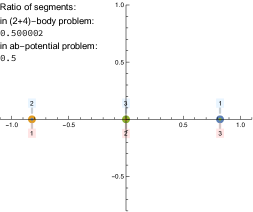
  (a) Horizontal.

  

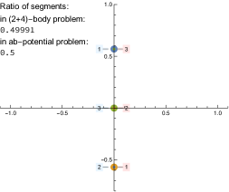
  (b) Vertical.

  Figure 6: Collinear solutions.

  Coordinates of the collinear solutions in the (2+3)-body problem, normalized by (85) and coordinates in $ab$-potential are given below:

  $$\begin{array}[]{m{1em}|c|rr|rr}&q_{i}&\lx@intercol\hfil\mbox{PGU normalized coordinates}\hfil\lx@intercol&\lx@intercol\hfil\mbox{PHU coordinates (in $ab$-potential)}\hfil\lx@intercol\\ \hline\cr\hbox{\multirowsetup\rotatebox{90.0}{horizontal\leavevmode\nobreak\ \leavevmode\nobreak\ }}&q_{1}&(-0.822075,&0.000685358)&(-0.8220706914,&0.0000000000)\\ &q_{2}&(0.822075,&0.000685548)&(0.8220706914,&0.0000000000)\\ &q_{3}&(-4.17619\times 10^{-17},&-0.00137091)&(0.0000000000,&-0.0000000000)\\ \hline\cr\hbox{\multirowsetup\rotatebox{90.0}{vertical\leavevmode\nobreak\ \leavevmode\nobreak\ \leavevmode\nobreak\ }}&q_{1}&(7.11379\times 10^{-8},&-0.569958)&(0.0000000000,&0.5699919822)\\ &q_{2}&(-7.11379\times 10^{-8},&0.570128)&(-0.0000000000,&-0.5699919822)\\ &q_{3}&(0.0,&-0.0000681896)&(0.0000000000,&0.0000000000)\\ \end{array}$$

• Figure 6 displays the Isosceles triangle solutions found.

  

  

  Figure 6: Triangle solutions.

  Coordinates of the isosceles triangle in the (2+3)-body problem, normalized by (85) and coordinates in $ab$-potential are given below:

  $$\begin{array}[]{m{1em}|c|rr|rr}&q_{i}&\lx@intercol\hfil\mbox{PGU normalized coordinates}\hfil\lx@intercol&\lx@intercol\hfil\mbox{PHU coordinates (in $ab$-potential)}\hfil\lx@intercol\\ \hline\cr\hbox{\multirowsetup\rotatebox{90.0}{triangle\leavevmode\nobreak\ \leavevmode\nobreak\ \leavevmode\nobreak\ }}&q_{1}&(-0.696414,&-0.000092914)&(-0.6964118400,&0.0000000000)\\ &q_{2}&(0.347844,&0.346726)&(0.3482059200,&0.3466806372)\\ &q_{3}&(0.34857,&-0.346634)&(0.3482059200,&-0.3466806372)\end{array}$$

7.4.2 $k=4$

PGU is run for data with two big masses being close to $\frac{1}{2}\left(1-2\cdot 10^{-5}\right)$ and four small masses $\mu_{i}=5\cdot 10^{-6}$ for $i=1,\dots,4$; PHU for masses $\tilde{\mu}_{i}=1/4$ for $i=1,\dots,4$. The initial boxes for light bodies in PGU are placed at $[-0.2,0.2]\times[0.8,0.9]$, first heavy body is placed at $[0.45,0.55]\times 0$, second is computed by the center of mass. In both programs PHU and PGU we obtained the same number of solutions and we were able to pair to the solutions from both programs as suggested by Theorem 11.

We obtained $10\cdot 4!=240$ solutions,

• collinear on the $x$ axis, $4!$ solutions

• collinear on the $y$ axis, $4!$ solutions

• isosceles triangle with fourth point close to the base symmetric with respect to the $x$ axis and its reflection with respect to the $y$ axis (see Fig. 6), $2\cdot 4!$ solutions

• equilateral triangle inside the isosceles one symmetric with respect to the $x$ axis and its reflection with respect to the $y$ axis (see Fig. 6), $2\cdot 4!$ solutions

• rhombus symmetric with respect to the $x$ and $y$ axes, (see Fig. 7), $4!$ solutions

• rectangle symmetric with respect to the $x$ and $y$ axes (see Fig. 8), $4!$ solutions

• ‘slanted’ rhombus and its symmetric image coordinate axes (see Fig. 8), $2\cdot 4!$ solutions

Comparison of solutions

• horizontally and vertically collinear (two solutions)

  

  

  Figure 6: Collinear solutions.

• isosceles triangle

  

  

  Figure 6: Isosceles triangles.

• equilateral triangle inside the isosceles one

  

  

  Figure 6: Equilateral triangle inside the isosceles one.

• rhombus symmetric with respect to the $x$ and $y$ axes

  

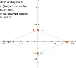
  Figure 7: Rhombus solution.

• rectangle symmetric with respect to the $x$ and $y$ axes

  

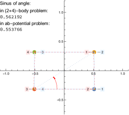
  Figure 8: Rectangle.

• ‘slanted’ rhombus

  

  

  Figure 8: ‘Slanted’ rhombuses.

Detailed comparison for symmetrical rhombus

From Theorem 18 we obtain the ratio of diagonals $k=0.39827$. From PGU we get $k=0.398089$ and from PHU — $k=0.39827$.

Coordinates of the rhombus in the (2+4)-body problem, normalized by (85), and coordinates in $ab$-potential are given below:

$$\begin{array}[]{m{1em}|c|rr|rr}&q_{i}&\lx@intercol\hfil\mbox{PGU normalized coordinates}\hfil\lx@intercol&\lx@intercol\hfil\mbox{PHU coordinates (in $ab$-potential)}\hfil\lx@intercol\\ \hline\cr&q_{1}&(0.0000117898,&-0.340306)&(0.0000000000,&-0.3392209571)\\ \hbox{\multirowsetup\rotatebox{90.0}{rhombus}}&q_{2}&(-0.852035,&0.00109155)&(-0.8517357111,&-0.0000000000)\\ &q_{3}&(-0.0000117106,&0.338064)&(-0.0000000000,&0.3392209571)\\ &q_{4}&(0.852034,&0.00115058)&(0.8517357111,&0.0000000000)\end{array}$$

Detailed comparison for rectangle

From Theorem 19, the angle between diagonal and the $x$ axis is $\varphi=0.553766$. From PGU we get $\varphi=0.562192$ and from PHU — $\varphi=0.553766$.

Normalized coordinates of the recatngle in the (2+4)-body problem and coordinates in $ab$-potential are given below:

$$\begin{array}[]{m{1em}|c|rr|rr}&q_{i}&\lx@intercol\hfil\mbox{PGU normalized coordinates}\hfil\lx@intercol\vrule\lx@intercol&\lx@intercol\hfil\mbox{PHU coordinates (in $a,b$-potential)}\hfil\lx@intercol\\ \hline\cr&q_{1}&(0.502676,&0.316689)&(0.5124981464,&0.3168767565)\\ \hbox{\multirowsetup\rotatebox{90.0}{rectangle}}&q_{2}&(0.522598,&-0.316654)&(0.5124981464,&-0.3168767565)\\ &q_{3}&(-0.522576,&-0.31669)&(-0.5124981464,&-0.3168767565)\\ &q_{4}&(-0.502698,&0.316654)&(-0.5124981464,&0.3168767565)\end{array}$$

In fact, in PGU the solution is a trapeziod, very close to being rectanglar.

Appendix A Technical proofs omitted in the main paper

A.1 Proof of Lemma 12

We show the identity (74a) — the proof of (74b) is analogous.

Notice that

$$\begin{array}[]{lclp{7cm}}x_{i}^{2}&=&x_{i}\left(x_{i}-\sum_{j}\mu_{j}x_{j}\right)&\quad\quad(since (\ref{eq:cc-cofmass}) implies $\sum_{i}\mu_{i}x_{i}=0$)\\ &=&x_{i}\left(x_{i}\sum_{j}\mu_{j}-\sum_{j}\mu_{j}x_{j}\right)&\quad\quad(use (\ref{eq:sum-mui}))\\ &=&x_{i}\left(\sum_{j}\mu_{j}(x_{i}-x_{j})\right)&\end{array}$$

Now we obtain

$$\sum_{i}\mu_{i}x_{i}^{2} = \sum_{i}\sum_{j}\mu_{i}\mu_{j}(x_{i}^{2}-x_{i}x_{j})$$

$$= \sum_{i<j}\mu_{i}\mu_{j}(x_{i}^{2}-2x_{i}x_{j}+x_{j}^{2})$$

$$= \sum_{i<j}\mu_{i}\mu_{j}(x_{i}-x_{j})^{2}$$

On the other hand

$$\sum_{i}\mu_{i}ax_{i}^{2} = \sum_{i}\sum_{j,j\neq i}\frac{\mu_{i}\mu_{j}(x_{i}-x_{j})x_{i}}{r_{ij}^{3}}\quad\quad(\mbox{by}\leavevmode\nobreak\ (\ref{eqn:a-b}))$$

$$= \sum_{i<j}\frac{\mu_{i}\mu_{j}}{r_{ij}^{3}}(x_{i}-x_{j})^{2}$$

From (74a, 74b) the equation (74c) is obvious:

$$a\left(\sum_{i}\mu_{i}x_{i}^{2}\right)+b\left(\sum_{i}\mu_{i}y_{i}^{2}\right) = \sum_{i<j}\frac{\mu_{i}\mu_{j}}{r_{ij}^{3}}(x_{i}-x_{j})^{2}+\sum_{i<j}\frac{\mu_{i}\mu_{j}}{r_{ij}^{3}}(y_{i}-y_{j})^{2}$$

$$= \sum_{i<j}\frac{\mu_{i}\mu_{j}}{r_{ij}}$$

∎

A.2 Proof of Lemma 14

From Lemma 12 we have

$$\max\{a,b\}\sum_{i}\mu_{i}(x_{i}^{2}+y_{i}^{2}) \geq a\left(\sum_{i}\mu_{i}x_{i}^{2}\right)+b\left(\sum_{i}\mu_{i}y_{i}^{2}\right)$$

$$= \sum_{i<j}\frac{\mu_{i}\mu_{j}}{r_{ij}}>\frac{\mu_{i}\mu_{j}}{r_{ij}}$$

From the above using (73) we obtain

$$r_{ij} > \frac{\mu_{i}\mu_{j}}{\max\{a,b\}\sum_{i}\mu_{i}(x_{i}^{2}+y_{i}^{2})}$$

$$> \frac{\mu_{i}\mu_{j}}{\max\{a,b\}R^{2}\sum_{i}\mu_{i}}$$

$$= \frac{\mu_{i}\mu_{j}}{\max\{a,b\}R^{2}}.$$

∎

A.3 Proof of Theorem 15

For the proof of Theorem 15 we will need the following result.

Lemma 20.

Let

$$M=\sum_{i}\mu_{i}.$$ (87)

Assume that $a>0$ or $b>0$. Assume $P_{k}^{\mu}$ is a solution of (71). Let $R=|x_{i_{0}}|=\max_{i}|x_{i}|$. If $a>0$, then for all $\varepsilon\in\left(0,R/(n-1)\right)$ holds

$$R-(n-2)\varepsilon<\frac{M}{a\varepsilon^{2}}.$$ (88)

Analogously, let $R=|y_{i_{0}}|=\max_{i}|y_{i}|$. If $b>0,then$ for all $\varepsilon\in\left(0,R/(n-1)\right)$ holds

$$R-(n-2)\varepsilon<\frac{M}{b\varepsilon^{2}}.$$ (89)

Proof.

Let us fix any $\varepsilon\in\left(0,R/(n-1)\right)$. We can assume that

$$p_{i_{0}}=(R,y_{i_{0}}).$$ (90)

Let $\mathcal{C}$ be a minimal subset (cluster) of indices of bodies satisfying the following conditions

• $i_{0}\in\mathcal{C}$

• if $j\in\mathcal{C}$ and $|p_{k}-p_{j}|\leqslant\varepsilon$, then $k\in\mathcal{C}$

The cluster $\mathcal{C}$ can be constructed as follows: We start with $i_{0}\in\mathcal{C}$. Then we add all bodies which are not farther than $\varepsilon$ from the bodies already in $\mathcal{C}$. We repeat this until the set $\mathcal{C}$ stabilizes, which happens after at most $n-1$ steps. From assumption about $\varepsilon$ and $R$ it follows that

$$R>(n-1)\varepsilon.$$ (91)

Observe that (91) implies that $\mathcal{C}\neq\{1,\dots,n\}$. Indeed (91) and (90) imply that $x_{i}>0$ for all $i\in\mathcal{C}$. This and the center of mass condition (72) implies that $\mathcal{C}$ cannot contain all bodies. This implies that the process of building $\mathcal{C}$ must stop after at most $n-2$ steps. Therefore we obtained a cluster $\mathcal{C}$ with the following properties

$$p_{i} \in \overline{B(p_{i_{0}},(n-2)\varepsilon)},\quad\forall i\in\mathcal{C},$$ (92)

$$|p_{i}-p_{j}| > \varepsilon,\quad i\in\mathcal{C},j\notin\mathcal{C}.$$ (93)

Figure 9: $R>(n-1)\varepsilon$ and $r=(n-2)\varepsilon$; the darkened area is the region where all the bodies from cluster are located.

Note that

$$\sum_{\begin{subarray}{c}i,j\in\mathcal{C}\\ i\neq j\end{subarray}}\frac{\mu_{i}\mu_{j}}{r_{ij}^{3}}(x_{i}-x_{j})=0$$

thus by adding equations for $x$’s in (71) for $i\in\mathcal{C}$ we obtain

$$a\sum_{i\in\mathcal{C}}\mu_{i}x_{i} = \sum_{\begin{subarray}{c}i,j\in\mathcal{C}\\ i\neq j\end{subarray}}\frac{\mu_{i}\mu_{j}(x_{i}-x_{j})}{r_{ij}^{3}}+\sum_{\begin{subarray}{c}i\in\mathcal{C}\\ j\not\in\mathcal{C}\end{subarray}}\frac{\mu_{i}\mu_{j}(x_{i}-x_{j})}{r_{ij}^{3}}.$$ (94)

Let

$$\mu_{\mathcal{C}} = \sum_{i\in\mathcal{C}}\mu_{i},$$

$$c_{\mathcal{C}} = \frac{1}{\mu_{\mathcal{C}}}\sum_{i\in\mathcal{C}}\mu_{i}x_{i},$$

$$F_{\mathcal{C}} = \frac{1}{\mu_{\mathcal{C}}}\sum_{\begin{subarray}{c}i\in\mathcal{C}\\ j\not\in\mathcal{C}\end{subarray}}\frac{\mu_{i}\mu_{j}(x_{i}-x_{j})}{r_{ij}^{3}}.$$

Observe that (94) could be now rewritten as

$$a\cdot c_{\mathcal{C}}=F_{\mathcal{C}}.$$ (95)

It is easy to see (cf. (92)) that for $i\in\mathcal{C}$: $x_{i}\geqslant R-(n-2)\varepsilon>0$, hence

$$|c_{\mathcal{C}}| = \frac{1}{\mu_{\mathcal{C}}}\sum_{i\in\mathcal{C}}\mu_{i}x_{i},$$

$$\geqslant R-(n-2)\varepsilon,$$

and

$$|F_{\mathcal{C}}| \leqslant \frac{1}{\mu_{\mathcal{C}}}\sum_{\begin{subarray}{c}i\in\mathcal{C}\\ j\not\in\mathcal{C}\end{subarray}}\frac{\mu_{i}\mu_{j}}{r_{ij}^{2}}\leqslant\frac{1}{\varepsilon^{2}}\frac{1}{\mu_{\mathcal{C}}}\sum_{\begin{subarray}{c}i\in\mathcal{C}\\ j\not\in\mathcal{C}\end{subarray}}\mu_{i}\mu_{j}$$

$$= \frac{1}{\varepsilon^{2}}\frac{1}{\mu_{\mathcal{C}}}\left(\sum_{i\in\mathcal{C}}\mu_{i}\right)\cdot\left(\sum_{j\notin\mathcal{C}}\mu_{j}\right)=\frac{1}{\varepsilon^{2}}\sum_{j\notin\mathcal{C}}\mu_{j}<\frac{M}{\varepsilon^{2}}.$$

Hence from the above and (95) we obtain

$$a(R-(n-2)\varepsilon)\leqslant|a\cdot c_{\mathcal{C}}|=|F_{\mathcal{C}}|<\frac{M}{\varepsilon^{2}}.$$

This completes the proof of (88). The proof of (89) is analogous.

∎

Proof‘of Theorem 15 We focus on the estimate on $R=\max_{i}|x_{i}|$. From Lemma 20 we have the following implication for any $\varepsilon$:

if $(n-1)\varepsilon<R$, then $R<(n-2)\varepsilon+\frac{M}{a\varepsilon^{2}}$.

Therefore

$$R\leq g(\varepsilon):=\max\left((n-1)\varepsilon,(n-2)\varepsilon+\frac{M}{a\varepsilon^{2}}\right).$$ (96)

We look for minimum of $g(\varepsilon)$. It is easy to see that

$$g(\varepsilon) = (n-1)\varepsilon,\quad\mbox{for $\varepsilon\geq\left(\frac{M}{a}\right)^{1/3}$},$$

$$g(\varepsilon) = g_{2}(\varepsilon):=(n-2)\varepsilon+\frac{M}{a\varepsilon^{2}},\quad\mbox{for $\varepsilon\leq\left(\frac{M}{a}\right)^{1/3}$}$$

The function $g_{2}(\varepsilon)$ has a global minimum at $\varepsilon_{0}=\left(\frac{2M}{(n-2)a}\right)^{1/3}$ and

$$g(\varepsilon_{0})=\left(\frac{M}{a}\right)^{1/3}\left(2^{1/3}+2^{-2/3}\right)(n-2)^{2/3}$$

Now $\varepsilon_{0}\leq\left(\frac{M}{a}\right)^{1/3}$ iff $n\geq 4$, therefore

$$\min g(\varepsilon)=(n-1)\left(\frac{M}{a}\right)^{1/3},\quad\mbox{for $n\geq 2$},$$

$$\min g(\varepsilon)=\left(\frac{M}{a}\right)^{1/3}\left(2^{1/3}+2^{-2/3}\right)(n-2)^{2/3},\quad\mbox{for $n\geq 4$}.$$

∎

A.4 Proof of Theorem 16

We divide by $\mu_{i}$ the equations (71) and take differences for $x_{i}$’s and $y_{i}$’s separately. Then we obtain system (71) written in matrix form as

$$A\begin{bmatrix}x_{1}-x_{2}\\ x_{2}-x_{3}\\ \ldots\\ x_{k-1}-x_{k}\end{bmatrix}=a\begin{bmatrix}x_{1}-x_{2}\\ x_{2}-x_{3}\\ \ldots\\ x_{k-1}-x_{k}\end{bmatrix} A\begin{bmatrix}y_{1}-y_{2}\\ y_{2}-y_{3}\\ \ldots\\ y_{k-1}-y_{k}\end{bmatrix}=b\begin{bmatrix}y_{1}-y_{2}\\ y_{2}-y_{3}\\ \ldots\\ y_{k-1}-y_{k},\end{bmatrix}$$ and (97)

where $A\in\mathbb{R}^{(k-1)\times(k-1)}$ is matrix with

$$A_{ij} = -\delta_{ij}-\chi_{[1,i-1]}(j)\left(\sum_{t=1}^{j}\frac{\mu_{t}}{r_{it}^{3}}\right)+\chi_{[i,n-1]}(j)\left(\sum_{t=j+1}^{k}\frac{\mu_{t}}{r_{it}^{3}}\right)$$

$$+\chi_{[1,i]}(j)\left(\sum_{t=1}^{j}\frac{\mu_{t}}{r_{(i+1)t}^{3}}\right)-\chi_{[i+1,n-1]}(j)\left(\sum_{t=j+1}^{k}\frac{\mu_{t}}{r_{(i+1)t}^{3}}\right),$$

where $\delta_{ij}$ is Kronecker delta and $\chi_{[l,p]}$ is the characteristic function of the interval $[l,p]$, i.e.

$$\chi_{[l,p]}(j)=\left\{\begin{array}[]{ll}1,&l\leq j\leq p\\ 0,&\mbox{otherwise}\end{array}\right.$$

For example, matrix $A$ for $k=3$ is:

$$A=\begin{bmatrix}\frac{\mu_{1}+\mu_{2}}{r_{12}^{3}}+\frac{\mu_{3}}{r_{13}^{3}},&\mu_{3}\left(\frac{1}{r_{13}^{3}}-\frac{1}{r_{23}^{3}}\right)\\ \mu_{1}\left(\frac{1}{r_{13}^{3}}-\frac{1}{r_{12}^{3}}\right),&\frac{\mu_{2}+\mu_{3}}{r_{23}^{3}}+\frac{\mu_{1}}{r_{13}^{3}}\\ \end{bmatrix}.$$

Observe from (97) we see that for any solution of (71) the $x$-differences and $y$-differences are eigenvectors of $A$ of different eigenvalues $a,b$, respectively or are zero. This with collinearity assumption implies that the solution must be on the coordinate axis. The precise argument goes as follows.

From collinearity it follows that there exist $\lambda_{i}\neq 0$, $i=2,\ldots,k-1$ such that

$$[x_{i}-x_{i+1},y_{i}-y_{i+1}]=\lambda_{i}[x_{1}-x_{2},y_{1}-y_{2}].$$

For the proof it is enough to show that $x_{1}-x_{2}=0$ or $y_{1}-y_{2}=0$.

We have

$${}[x_{1}-x_{2},x_{2}-x_{3},\dots,x_{k-1}-x_{k}] = (x_{1}-x_{2})[1,\lambda_{2},\dots,\lambda_{k-1}],$$

$${}[y_{1}-y_{2},y_{2}-y_{3},\dots,y_{k-1}-y_{k}] = (y_{1}-y_{2})[1,\lambda_{2},\dots,\lambda_{k-1}].$$

Let

$$\Lambda=[1,\lambda_{2},\dots,\lambda_{k-1}]^{t},$$

thus we have

$$A\left((x_{1}-x_{2})\Lambda\right)=a\left((x_{1}-x_{2})\Lambda\right),$$

$$A\left((y_{1}-y_{2})\Lambda\right)=b\left((y_{1}-y_{2})\Lambda\right)$$

Since $a\neq b$, then either $x_{1}-x_{2}=0$ or $y_{1}-y_{2}$. Hence we obtain our conclusion.

∎

A.5 Proof of Theorem 17

Since we are looking for an isosceles triangle symmetrical with respect to the $x$ axis and since the center of mass is at the origin, we can assume that

$$p_{1}=(x,0),\quad p_{2}=\left(-\frac{x}{2},y\right),\quad p_{3}=\left(-\frac{x}{2},-y\right)$$

where $x\neq 0$ and $y\neq 0$, since the solution cannot be collinear. Without loss of generality, assume $x,y>0$.

Figure 10: A sample isosceles triangle with $x,y>0$.

Then we have

$$r=r_{23}=2y,\quad s=r_{12}=r_{13}=\sqrt{\frac{9x^{2}}{4}+y^{2}}.$$ (98)

From the above, it is easy to see that the system (71) can be reduced to

$$ax =\frac{3\mu x}{r_{12}^{3}},$$ (99a)

$$by =\frac{\mu y}{r_{12}^{3}}+\frac{2\mu y}{r_{23}^{3}}.$$ (99b)

Since $x\neq 0$ and $y\neq 0$, we obtain

$$a = \frac{3\mu}{r_{12}^{3}},$$

$$b = \frac{\mu}{r_{12}^{3}}+\frac{2\mu}{r_{23}^{3}}.$$

Hence

$$r_{12}^{3} =\frac{3\mu}{a},$$ (100a)

$$r_{23}^{3} =\frac{2\mu}{b-\frac{a}{3}},$$ (100b)

For the equation (100b) to make sense, the denominator must be positive ($r=r_{23}>0$), thus

$$b>\frac{a}{3}.$$ (101)

Note that (101) is compatibile with the assumtion (78). From (98) we compute

$$y^{3} =\frac{\mu}{4(b-\frac{a}{3})},$$ (102a)

$$x^{2} =\left(\frac{2}{3}\right)^{2}(r_{12}^{2}-y^{2}).$$ (102b)

To have a real solution, we demand $r_{12}^{2}-y^{2}>0$, which implies (78). ∎

A.6 Proof of Theorem 18

Assume that the rhombus is as on the figure below:

$$p_{1}=(x,0)\quad p_{2}=(0,y)\quad p_{3}=(-x,0)\quad p_{4}=(0,-y),$$

where $x>0$ and $y>0$. Ratio of diagonals is $k=y/x>0$.

It is easy to see that the system (71) can be reduced to the following two equations

$$a =\mu\frac{2}{r^{3}}+\mu\frac{1}{4x^{3}}$$ (103a)

$$b =\mu\frac{2}{r^{3}}+\mu\frac{1}{4y^{3}}.$$ (103b)

Since $y=kx$, it holds that $r=x\sqrt{1+k^{2}}$ and we can wrtite

$$a =\frac{\mu}{x^{3}}\left(\frac{2}{(\sqrt{(1+k^{2})})^{3}}+\frac{1}{4}\right)$$ (104a)

$$b =\frac{\mu}{x^{3}}\left(\frac{2}{(\sqrt{(1+k^{2})})^{3}}+\frac{1}{4k^{3}}\right).$$ (104b)

Dividing the corresponding sides of (104a) and (104b) we obtain (79). The lhs of (79),

$$f(k)=\frac{8k^{3}+k^{3}(\sqrt{1+k^{2}})^{3}}{(\sqrt{1+k^{2}})^{3}+8k^{3}},$$

is strictly increasing, $\lim_{k\to\infty}f(k)=\infty$ and $f(0)=0$, so equation (79) has exactly one solution (see Fig. 11).

By (103a) we have

$$a = \mu\frac{2}{r^{3}}+\mu\frac{1}{4x^{3}}>\mu\frac{2}{r^{3}}+\mu\frac{1}{4r^{3}}=\frac{9\mu}{4r^{3}},$$ (105)

and analogously from (103b) we obtain

$$b>\frac{9\mu}{4r^{3}}.$$ (106)

Combining (105) and (106) we get the lower bound for $r$, namely

$$r^{3}>\max\left(\frac{9\mu}{4a},\frac{9\mu}{4b}\right)=\frac{9\mu}{4\min(a,b)}.$$ (107)

And again using (103), we compute $x^{2}$ and $y^{2}$:

$$x^{2} = r^{2}\left(\frac{\mu}{4(ar^{3}-2\mu)}\right)^{\frac{2}{3}}$$

$$y^{2} = r^{2}\left(\frac{\mu}{4(br^{3}-2\mu)}\right)^{\frac{2}{3}}.$$

Observe that from (107) it follows that denominators in the above equations are positive.

Hence

$$r^{2}=x^{2}+y^{2}=r^{2}\left(\frac{\mu}{4(ar^{3}-2\mu)}\right)^{\frac{2}{3}}+r^{2}\left(\frac{\mu}{4(br^{3}-2\mu)}\right)^{\frac{2}{3}}$$

and we obtain (80). Using lhs of (80) we define a function

$$g_{1}(r)=\left(\frac{2\mu}{ar^{3}-2\mu}\right)^{\frac{2}{3}}+\left(\frac{2\mu}{br^{3}-2\mu}\right)^{\frac{2}{3}}.$$

The equation (80) has exactly one solution, with $r>\displaystyle{\left(\frac{2\mu}{\min\{a,b\}}\right)^{1/3}}$ (see Fig. 12)

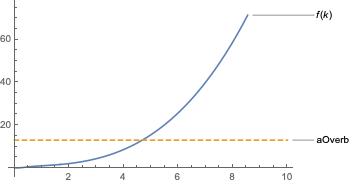
Figure 11: Function $f$ of a ratio of diagonals $k$. Yellow dashed line is at $a/b$.

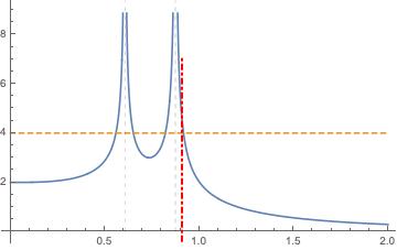
Figure 12: Function $g_{1}$ of a size of sides $r$. Asymptotes (dashed vertical lines) are at $r=(2\mu/b)^{1/3}$ and $r=(2\mu/a)^{1/3}$; the lower bound for $r$ is marked as red line.

Figure 13: Functions describing geometry of the rhombus.

∎

A.7 Proof of Theorem 19

Assume that the rectangle is as on the figure below:

$$p_{1}=(x,y)\quad p_{2}=(x,-y)\quad p_{3}=(-x,-y)\quad p_{4}=(-x,y),$$

where $x,y>0,$ $x=r\cos(\varphi)$ and $y=r\sin(\varphi)$.

It is easy to see that the system (71) can be reduced to

$$a =\frac{\mu}{4}\left(\frac{1}{r^{3}}+\frac{1}{x^{3}}\right),$$ (108a)

$$b =\frac{\mu}{4}\left(\frac{1}{r^{3}}+\frac{1}{y^{3}}\right).$$ (108b)

and afterwards to

$$a = \frac{\mu}{4r^{3}}\left(1+\frac{1}{\cos^{3}(\varphi)}\right),$$

$$b = \frac{\mu}{4r^{3}}\left(1+\frac{1}{\sin^{3}(\varphi)}\right).$$

Diving the corresponding sides of above equations we obtain (81). The lhs of (81),

$$f(\varphi)=\frac{\sin^{3}(\varphi)(\cos^{3}(\varphi)+1)}{\cos^{3}(\varphi)(\sin^{3}(\varphi)+1)},$$

is strictly increasing for $\varphi\in[0,\pi/2)$, $\lim_{\varphi\to\pi/2}f(\varphi)=\infty$ and $f(0)=0$, so equation (81) has unique solution in $[0,\pi/2)$ (see Fig. 14).

By (108) we have

$$a = \frac{\mu}{4}\left(\frac{1}{r^{3}}+\frac{1}{x^{3}}\right)>\frac{9\mu}{4r^{3}}$$

$$b = \frac{\mu}{4}\left(\frac{1}{r^{3}}+\frac{1}{y^{3}}\right)>\frac{9\mu}{4r^{3}}$$

Combining above inequalities we get the lower bound for $r$. Again using (108), we compute $x^{2}$ and $y^{2}$:

$$x^{2} = r^{2}\left(\frac{\mu}{4ar^{3}-\mu}\right)^{\frac{2}{3}}$$

$$y^{2} = r^{2}\left(\frac{\mu}{4br^{3}-\mu}\right)^{\frac{2}{3}}$$

hence

$$r^{2}=x^{2}+y^{2}=r^{2}\left(\left(\frac{\mu}{4ar^{3}-\mu}\right)^{\frac{2}{3}}+\left(\frac{\mu}{4br^{3}-\mu}\right)^{\frac{2}{3}}\right)$$

and we obtain (82). Using lhs of (80) define a function

$$g_{2}(r)=\left(\frac{\mu}{4ar^{3}-\mu}\right)^{\frac{2}{3}}+\left(\frac{\mu}{4br^{3}-\mu}\right)^{\frac{2}{3}}.$$

The equation (82) has exactly one solution, with $r>(\mu/(4a))^{1/3}$ (see Fig. 15)

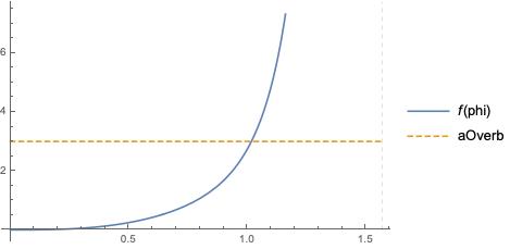
Figure 14: Function $f(\varphi)$; horizontal dashed line is at $a/b$. Note that, for any $a$, $b$ and $\varphi\in(0,\pi/2)$, the equation $f(\varphi)=a/b$ has exactly one solution.

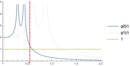
Figure 15: Function $g_{2}(r)$. Asymptotes (dashed vertical lines) are at $r=(\mu/(4a))^{1/3}$ and $r=(\mu/(4b))^{1/3}$; red dotted-dashed line illustrates the lower bound for $r$. Thin gray lines are the graph of function $g_{1}$ for rhombus.

Figure 16: Functions describing geometry of rectangle.

∎

A.8 Computation of $a,b$ at $L_{4}$ in the restricted three body problem

We assume that point of mass $m_{i}$ is located at $p_{i}$, $i=1,2$ where

$$p_{1}=\left(-1/2,0\right),\quad p_{2}=\left(1/2,0\right),$$

The masses are normalized to $m_{1}+m_{2}=1$. The zero-mass (third) body has an unknown location $z=(x,y)$. The equation for relative equilibria is $\nabla V(z;m)=0$, where

$$V(z;m)=\frac{1}{2}\|z-c\|^{2}+\sum_{i=1}^{3}m_{i}\|z-p_{i}\|^{-1}$$

where $c=\sum_{i=1}^{2}m_{i}p_{i}$ is the center of mass.

It is well known (see for example [MD]) that we have five relative equilibria: three collinear with the primaries (called $L_{1},L_{2},L_{3}$) and two triangular $L_{4}$ and $L_{5}$, which form an equilateral triangle with the primaries. $L_{4}$ and $L_{5}$ are mutually symmetric with respect to the line passing through the primaries. For any choice of positive masses $m_{1}$, $m_{2}$, such that $m_{1}+m_{2}=1$, we have $L_{4}=(0,\sqrt{3}/2)$ and $L_{5}=(0,-\sqrt{3}/2)$.

Expressions in the lemma below are computed using Mathematica program [Mth].

Lemma 21.

$$D^{2}V(L_{4})=\begin{bmatrix}\frac{3}{4}&\frac{3}{4}\sqrt{3}(2m_{1}-1)\\ \frac{3}{4}\sqrt{3}(2m_{1}-1)&\frac{9}{4}\\ \end{bmatrix}=\begin{bmatrix}\frac{3}{4}&\frac{3}{4}\sqrt{3}(m_{1}-m_{2})\\ \frac{3}{4}\sqrt{3}(m_{1}-m_{2})&\frac{9}{4}\\ \end{bmatrix}$$

The matrix $D^{2}V(L_{4})$ is positive definite. Its eigenvalues $\lambda_{1}>\lambda_{2}$ are given by

$$\lambda_{2} = \frac{3}{2}\left(1-\sqrt{3m_{1}^{2}-3m_{1}+1}\right)=\frac{3}{2}\left(1-\sqrt{1-3m_{1}m_{2}}\right),$$

$$\lambda_{1} = \frac{3}{2}\left(\sqrt{3m_{1}^{2}-3m_{1}+1}+1\right)=\frac{3}{2}\left(1+\sqrt{1-3m_{1}m_{2}}\right)$$

and satisfy the following conditions

$$\sqrt{3} > \lambda_{1}-\lambda_{2}\geq\frac{3}{2}$$

$$\lambda_{1} < \frac{3}{2}\left(1+\frac{1}{\sqrt{3}}\right),$$

$$\lambda_{2} = \frac{9m_{1}m_{2}}{4}+O((m_{1}m_{2})^{2}).$$

Proof.

Expressions for $\lambda_{1,2}$ can be checked by direct computation. It remains to establish the remaining inequalities. Since

$$3m_{1}^{2}-3m_{1}+1=3\left(\left(m_{1}-\frac{1}{2}\right)^{2}+\frac{1}{12}\right)=1-3m_{1}m_{2},$$

hence for $m_{1}\in(0,1)$ we obtain

$$\sqrt{3}>\lambda_{1}-\lambda_{2} = 3\sqrt{3m_{1}^{2}-3m_{1}+1}\geq\frac{3}{2}$$

$$\lambda_{1} < \frac{3}{2}\left(1+\frac{1}{\sqrt{3}}\right)$$

$$\lambda_{2} = \frac{3}{2}\left(1-\sqrt{1-3m_{1}m_{2}}\right)$$

$$= \frac{3}{2}\left(1-\left(1-\frac{3m_{1}m_{2}}{2}+O((m_{1}m_{2})^{2})\right)\right)$$

$$= \frac{9m_{1}m_{2}}{4}+O((m_{1}m_{2})^{2}).$$

∎

In particular for the case of equal masses we have

Lemma 22.

Assume that $m_{1}=m_{2}=1/2$. Then the eigenvalues of $D^{2}V(L_{4})$ are $\frac{3}{4}$ and $\frac{9}{4}$ with the eigenvectors $(1,0)$ and $(0,1)$, respectively.

References

- [AK12] A.Albouy V.Kaloshin, Finiteness of central configurations of five bodies in the plane, Annals of mathematics 176 (2012), 535–588
- [Al95] A.Albouy, Symmetry of central configurations of bodies, Comptes rendus de l’Academie des Sciences Serie I-Mathematique 320 (1995), 217–220
- [Al96] A.Albouy, The symmetric central configurations of four equal masses, Contemporary Mathematics 198 (1996), 131–135
- [A82] R. Arenstorf, Central configurations of four bodies with one inferior mass, Celestial Mechanics 28 (1982) 9-15
- [F02] D.Ferrario, Central configurations, symmetries and fixed points, arxiv.math/0204198v1, 2002
- [F07] D.Ferrario, Planar central configurations as fixed points. J. Fixed Point Theory Appl. 2 (2007), no. 2, 277–291.
- [HJ11] M.Hampton and A.N.Jensen, Finiteness of spatial central configurations in the five-body problem, Cel. Mech. Dyn. Astron. 109 (2011), no. 4, 321–332.
- [HM05] M.Hampton and R.Moeckel, Finiteness of relative equilibria of the four-body problem, Invent. math. 163 (2005), no. 2, 289–312.
- [K69] R.Krawczyk, Newton-Algorithmen zur Besstimmung von Nullstellen mit Fehlerschranken, Computing, 4(1969) , 187–201
- [Mth] The Software Engineering of Mathematica—Wolfram Mathematica 9 Documentation. Reference.wolfram.com.
- [MZ19] M.Moczurad, P.Zgliczyński, Central configurations in planar -body problem with equal masses for , Celestial Mechanics and Dynamical Astronomy, (2019) 131: 46
- [MZ20] M.Moczurad, P.Zgliczyński, Central configurations in spatial -body problem for with equal masses, Celestial Mechanics and Dynamical Astronomy, (2020) 132:56
- [Moe01] R.Moeckel, Generic finiteness for Dziobek configurations, Trans. Am. Math. Soc. 353, 4673–4686 (2001)
- [Moe89] R.Moeckel, Some Relative Equilibria of N Equal Masses , http://www-users.math.umn.edu/ rmoeckel/research/CC.pdf
-
[Moe]
R.Moeckel, Central configurations, Scholarpedia, 9(4):10667,
http://www.scholarpedia.org/article/Central_configurations - [Moe14] R.Moeckel, Lectures On Central Configurations, 2014, http://www-users.math.umn.edu/~rmoeckel/notes/CentralConfigurations.pdf
- [MD] C.D. Murray and S.F. Dermott, Solar System Dynamics, Cambrigde University Press, 1999
- [Mou] Moulton, F.R., The straight line solutions of the problem of N bodies. Annals of Math. Vol. 12, 1-17 (1910)
- [Si78] C.Simo, Relative equilibrium solutions in 4 body problem, Cel. Mech. Dyn. Astron. 18 (1978), 165–184
- [Sm] S. Smale, Topology and Mechanics II. The Planar n-Body Problem. Inventiones math. 11, 45-64 (1970)
- [Sm98] S.Smale, Mathematical problems for the next century, Mathematical Intelligencer 20 (1998), 7–15
- [W41] A.Wintner, The Analytical Foundations of Celestial Mechanics, Princeton, N.J. Princeton University Press, 1941
- [X91] Z. Xia, Central Configurations with Many Small Masses, Journal of Differential Equations 91, 168–179 (1991)