The Veneziano Amplitude
via Mostly BRST Exact Operator

The Veneziano amplitude is derived from fixing one degree of freedom of $PSL(2,\mathbb{R})$ symmetry by the insertion of a mostly BRST exact operator. Evaluating the five-point function which consists of four open string tachyons and this gauge fixing operator, we find it equals the Veneziano amplitude up to a sign factor. The sign factor is interpreted as a signed intersection number. The result implies that the mostly BRST exact operator, which is originally used to provide two-point string amplitudes, correctly fixes the $PSL(2,\mathbb{R})$ gauge symmetry for general amplitudes. We conjecture an expression for general $n$-point tree amplitudes with an insertion of this gauge fixing operator.

17 September 2021

1 Introduction

Two-point open string tree amplitude is revealed to have a non-zero result, although the amplitude is divided by the volume of the $PSL(2,\mathbb{R})$ symmetry with three degrees of freedom. In [1], it was shown that the two degrees of freedom lead to fixing of the positions of two vertex operators of the amplitude and the infinite volume of the residual symmetry is canceled by the delta function for energy conservation, which is constantly infinite due to momentum conservation and on-shell conditions. The resulting amplitude coincides with standard free particle expression in quantum field theories.

In the BRST formalism, a part of the present authors provided the same result for the two-point string amplitudes in [2] by introducing the BRST invariant operator which fixes the residual gauge symmetry. According to [3], the operator is defined by

$${\mathpzc E}(z)\equiv\frac{1}{\pi}\int_{-\infty}^{\infty}dq\,\Bigl{(}c\partial X^{0}e^{-iqX^{0}}-i\alpha^{\prime}q(\partial c)e^{-iqX^{0}}\Bigr{)}.$$ (1.1)

Here $X^{0}(z,\bar{z})$ is the string coordinate in the time direction, $c(z)$ is the ghost field, and $z$ is a point on the boundary. This operator can be rewritten by a mostly BRST exact expression:

$${\mathpzc E}(z)=\frac{1}{\pi}\int_{-\infty}^{\infty}dq\,\frac{i}{q}\,\delta_{\rm B}e^{-iqX^{0}}\,,\quad\delta_{\rm B}e^{-iqX^{0}}=[\,Q_{\rm B},\,e^{-iqX^{0}}\,]\,,$$ (1.2)

where $Q_{\rm B}$ is the BRST operator. For $q\neq 0$, the integrand is indeed BRST exact, but it is not so at $q=0$. Despite depending only on the time direction and being not on-shell, the operator is Lorentz and conformal invariant up to BRST exact operators [2]. The two-point amplitude is given by calculating the three-point function in which two arbitrary on-shell open string vertex operators and the operator $\mathpzc{E}(z)$ are inserted on the worldsheet.

It has been found that mostly BRST exact operators can be applied to superstring theory. In [4], a mostly BRST exact operator is constructed in the pure spinor formalism, by which two-point superstring amplitudes is shown to be equal to the corresponding expression in the field theories.

As for multipoint amplitudes, a correct three-point amplitude is derived in [3] from the four-point function with the insertions of three on-shell vertex operators and one ${\mathpzc E}$. In this derivation, the Feynman $i\varepsilon$ prescription plays an important role in extracting the singularity for a momentum of ${\mathpzc E}$, which only contributes to a physical result. In [3], two-point amplitude is also calculated by a different way in which double of ${\mathpzc E}$ are inserted, namely one position of the physical vertex is integrated in a four-point function. In this case, the $i\varepsilon$ prescription is also important to remove the integration of the position, and we thus obtain the correct two-point amplitude.

The $i\varepsilon$ prescription has relation to Minkowski nature of spacetime. In Minkowski spacetime, we deal with time differently than the spatial dimensions, and this is reflected in the representation of ${\mathpzc E}$, which includes the time direction only. For the $i\varepsilon$ prescription in string theories, it is significant that the string worldsheet also should be regarded to have Lorentz signature. Based on this principle, it is possible to introduce $i\varepsilon$ in the representation of amplitudes in terms of the moduli integral [5].

The mostly BRST exact operator (1.1) is expected to fix a part of $PSL(2,\mathbb{R})$ symmetry correctly, as found in [2] and [3]. However, it is difficult to derive general multipoint string amplitudes explicitly from correlation functions with ${\mathpzc E}$. The purpose of this paper is to derive the Veneziano amplitude [6], which includes one modulus, from a five-point function with one insertion of ${\mathpzc E}$. Consequently, we show that the mostly BRST exact operator and the $i\varepsilon$ prescription yield the Veneziano amplitude correctly.

We begin in subsection 2.1 with fixing the $PSL(2,\mathbb{R})$ symmetry that appears in the four-point open string tachyon amplitude by the use of ${\mathpzc E}$. As a result, we obtain a five-point function represented by the two cross-ratios, which are the same parameters of a five-point open string amplitude [7, 8] or the five-point case of the Koba-Nielsen amplitude [9]. Then we decompose the integration region into 12 components depending on the order of the vertices. To introduce $i\varepsilon$ to the five-point function, we have to understand details of the moduli space of the five-point function. In subsection 2.2, we illustrate the moduli space, particularly its coordinates, for one of the 12 components in reference to the results in [10], where the moduli space of the five-point function has been extensively studied to give a contour integral expression for that. Then, we introduce $i\varepsilon$ to a five-point function for this domain and extract the singularity contributing to the Veneziano amplitude. For the rest of the 12 components, we have only to repeat the same analysis as that of this domain and the details of calculations are in appendix A. Finally, combining these results in subsection 2.3, we obtain the Veneziano amplitude by the insertion of ${\mathpzc E}$; however, the resulting amplitude includes the sign factor depending on the energy of external states. As discussed in [3], this factor is interpreted by a signed intersection number associated with the string time coordinate $X^{0}$. Section 3 is dedicated to a conclusion and remarks on the extension to general multipoint amplitudes.

2 The Veneziano amplitude from a five-point function

2.1 Decomposition of a five-point function

Let us consider a four open string tachyon amplitude by inserting the vertex operators on the real axis of the upper-half plane as the worldsheet. For simplicity, the target space is taken as the 26-dimensional flat Minkowski spacetime.

The amplitude is defined formally by the integrals,

$$A_{4}=\frac{1}{{\rm vol}PSL(2,\mathbb{R})}\big{<}\int dy_{1}V_{1}(y_{1})\int dy_{2}V_{2}(y_{2})\int dy_{3}V_{3}(y_{3})\int dy_{4}V_{4}(y_{4})\big{>},$$ (2.1)

where $V_{i}$ is an open string vertex operator, $\big{<}\cdots\big{>}$ denotes a correlation function in the upper-half plane, and each integration is over the whole real line. ${\rm vol}PSL(2,\mathbb{R})$ is the volume of the conformal Killing group after fixing the worldsheet to the upper-half plane.

To fix the gauge symmetry of $PSL(2,\mathbb{R})$, we fix the positions $y_{3}$, $y_{4}$ ($y_{3}<y_{4}$) and their integrations are replaced by the ghost fields $c(y_{3})$, $c(y_{4})$. Here one degree of freedom of $PSL(2,\mathbb{R})$ remains unfixed. We fix this residual symmetry by the mostly BRST exact operator inserted at $y_{0}$. In the following, we suppose that the points $y_{0}$, $y_{3}$ and $y_{4}$ are in the order $y_{0}<y_{3}<y_{4}$, since the order affects only on the overall sign of the amplitude. For this gauge fixing, the amplitude (2.1) becomes

$${\cal A}_{4}=ig_{\rm o}^{4}C_{D_{2}}\!\left<0\right|{\mathpzc E}(y_{0})\int_{-\infty}^{\infty}dy_{1}V_{1}(y_{1})\int_{-\infty}^{\infty}dy_{2}V_{2}(y_{2})\,cV_{3}(y_{3})\,cV_{4}(y_{4})\left|0\right>\!,$$ (2.2)

where $C_{D_{2}}$ is a normalization factor for disk amplitudes: $C_{D_{2}}=1/(\alpha^{\prime}g_{\rm o}^{2})$ [11]. The open string coupling $g_{\rm o}$ is assigned to each vertex operator, but not to ${\mathpzc E}$ [3]. $\left|0\right>\!$ is the $SL(2,\mathbb{R})$ invariant vacuum normalized as $\langle 0|0\rangle=(2\pi)^{26}\delta^{26}(0)$. We note that $A_{4}$ and ${\cal A}_{4}$ are different in the sign as discussed in [3]. Using the expression (1.2) for $\mathpzc E$, we rewrite the amplitude as the $q$-integral of a correlation function:

$${\cal A}_{4} =ig_{\rm o}^{4}C_{D_{2}}\int_{-\infty}^{\infty}dq\,{\cal F}(q),$$

$${\cal F}(q) \equiv\!\left<0\right|\Big{(}\frac{i}{\pi q}\delta_{\rm B}e^{-iqX^{0}}(y_{0})\Big{)}\int_{-\infty}^{\infty}dy_{1}V_{1}(y_{1})\int_{-\infty}^{\infty}dy_{2}V_{2}(y_{2})\,cV_{3}(y_{3})cV_{4}(y_{4})\left|0\right>\!.$$ (2.3)

For simplicity, we consider the amplitude for open string tachyons, that is

$$V_{i}(y)\equiv e^{ip_{i}\cdot X}(y).$$ (2.4)

As in [3], we denote $e^{-iqX^{0}}$ in (1.2) as $e^{ip_{0}\cdot X}$ by introducing a covariant expression for the momentum $q$: $p_{0}=(q,0,\cdots,0)$. One can calculate the correlation function ${\cal F}(q)$,

$${\cal F}(q) =(2\pi)^{26}\delta^{26}\big{(}\sum_{k=0}^{4}p_{k}\big{)}\int_{-\infty}^{\infty}dy_{2}\int_{-\infty}^{\infty}dy_{1}\,\frac{i}{\pi q}\Big{\{}y_{03}y_{04}y_{34}$$

$$\quad\times\left(\frac{\alpha^{\prime}p_{0}\cdot p_{1}}{y_{01}}+\frac{\alpha^{\prime}p_{0}\cdot p_{2}}{y_{02}}+\frac{\alpha^{\prime}p_{0}\cdot p_{3}}{y_{03}}+\frac{\alpha^{\prime}p_{0}\cdot p_{4}}{y_{04}}\right)$$

$$\quad+\frac{\alpha^{\prime}}{2}p_{0}\cdot p_{0}(y_{03}y_{34}+y_{04}y_{34})\Big{\}}\times\prod_{i<j}|y_{ij}|^{2\alpha^{\prime}p_{i}\cdot p_{j}},$$ (2.5)

where $y_{ij}\equiv y_{i}-y_{j}$. Moreover, it is easily found that ${\cal F}(q)$ is rewritten as

$${\cal F}(q) =(2\pi)^{26}\delta^{26}\big{(}\sum_{k=0}^{4}p_{k}\big{)}\int_{-\infty}^{\infty}dy_{2}\int_{-\infty}^{\infty}dy_{1}\,\frac{-i}{2\pi q}\sum_{k=1}^{2}\frac{\partial}{\partial y_{k}}\Big{(}y_{k3}y_{k4}y_{34}\prod_{i<j}|y_{ij}|^{2\alpha^{\prime}p_{i}\cdot p_{j}}\Big{)}.$$ (2.6)

This expression implies that ${\cal F}(q)$ is generically zero since the integrand is given by the total derivative, but that is not the case for $q=0$ owing to the reciprocal factor of $q$. It is the result of the Ward-Takahashi identity for the BRST symmetry. Therefore, in calculating the amplitude, we have only to evaluate the singularity of ${\cal F}(q)$ at the support $q=0$.

In order to extract the singularity at $q=0$, it is necessary to represent the amplitude by a moduli integral[3]. Next, let us rewrite ${\cal F}(q)$ using moduli parameters, which are that of a five-point function, although calculating a four-point open string amplitude. We note that, for $q\neq 0$, ${\cal F}(q)$ is not invariant under $PSL(2,\mathbb{R})$ transformation since the energy $q$ is integrated in ${\cal F}(q)$ and there is no on-shell condition for the momentum of ${\mathpzc E}$. So we will not use $PSL(2,\mathbb{R})$ symmetry to express ${\cal F}(q)$ by moduli, unlike the conventional case.

The moduli space of a five-point function has real dimension 2. First, we choose the following two cross-ratios as the coordinate of the moduli space:

$$u_{1}=\frac{y_{01}y_{34}}{y_{03}y_{14}},~{}~{}~{}u_{2}=\frac{y_{02}y_{34}}{y_{03}y_{24}}.$$ (2.7)

From (2.7), it follows that

$$dy_{1}dy_{2}=du_{1}du_{2}\,\Big{|}\frac{y_{03}y_{14}y_{24}}{y_{04}y_{34}}\Big{|}^{2},$$ (2.8)

and, by using momentum conservation and on-shell conditions, components in the integrand of (2.5) can be rewritten as

$$\Big{\{}y_{03}y_{04}y_{34}\left(\frac{\alpha^{\prime}p_{0}\cdot p_{1}}{y_{01}}+\frac{\alpha^{\prime}p_{0}\cdot p_{2}}{y_{02}}+\frac{\alpha^{\prime}p_{0}\cdot p_{3}}{y_{03}}+\frac{\alpha^{\prime}p_{0}\cdot p_{4}}{y_{04}}\right)+\frac{\alpha^{\prime}}{2}p_{0}\cdot p_{0}(y_{03}y_{34}+y_{04}y_{34})\Big{\}}$$

$$=y_{34}^{2}\,\Big{(}\frac{\alpha^{\prime}p_{0}\cdot p_{0}}{2}+\alpha^{\prime}p_{0}\cdot p_{3}+\frac{\alpha^{\prime}p_{0}\cdot p_{1}}{u_{1}}+\frac{\alpha^{\prime}p_{0}\cdot p_{2}}{u_{2}}\Big{)},$$ (2.9)

$$\prod_{i<j}|y_{ij}|^{2\alpha^{\prime}p_{i}\cdot p_{j}} =\Big{|}\frac{y_{03}y_{14}y_{24}}{y_{04}}\Big{|}^{-2}\Big{|}\frac{y_{03}y_{04}}{y_{34}}\Big{|}^{-\alpha^{\prime}p_{0}\cdot p_{0}}$$

$$\quad\times|u_{1}|^{2\alpha^{\prime}p_{0}\cdot p_{1}}|1-u_{1}|^{2\alpha^{\prime}p_{1}\cdot p_{3}}|u_{2}|^{2\alpha^{\prime}p_{0}\cdot p_{2}}|1-u_{2}|^{2\alpha^{\prime}p_{2}\cdot p_{3}}|u_{1}-u_{2}|^{2\alpha^{\prime}p_{1}\cdot p_{2}}.$$ (2.10)

Substituting (2.8), (2.9) and (2.10) into (2.5), we obtain

$${\cal F}(q) =(2\pi)^{26}\delta^{26}\big{(}\sum_{k=0}^{4}p_{k}\big{)}\,\Big{|}\frac{y_{03}y_{04}}{y_{34}}\Big{|}^{\alpha^{\prime}q^{2}}\int^{\infty}_{-\infty}du_{2}\int^{\infty}_{-\infty}du_{1}\,\frac{i}{\pi q}$$

$$\quad\times\Big{(}\frac{\alpha^{\prime}p_{0}\cdot p_{0}}{2}+\alpha^{\prime}p_{0}\cdot p_{3}+\frac{\alpha^{\prime}p_{0}\cdot p_{1}}{u_{1}}+\frac{\alpha^{\prime}p_{0}\cdot p_{2}}{u_{2}}\Big{)}$$

$$\quad\times|u_{1}|^{2\alpha^{\prime}p_{0}\cdot p_{1}}|1-u_{1}|^{2\alpha^{\prime}p_{1}\cdot p_{3}}|u_{2}|^{2\alpha^{\prime}p_{0}\cdot p_{2}}|1-u_{2}|^{2\alpha^{\prime}p_{2}\cdot p_{3}}|u_{1}-u_{2}|^{2\alpha^{\prime}p_{1}\cdot p_{2}}.$$ (2.11)

The expression (2.11) corresponds to the correlation function which is derived from the transformation of the positions $y_{0}$, $y_{1}$, $y_{2}$, $y_{3}$ and $y_{4}$ to $0$, $u_{1}$, $u_{2}$, $1$ and $\infty$, respectively. This $PSL(2,\mathbb{R})$ transformation is given by

$$f(z)=-\frac{y_{34}(z-y_{0})}{y_{03}(z-y_{4})}.$$ (2.12)

It turns out that the factor with the exponent $\alpha^{\prime}q^{2}$ is given as $|f^{\prime}(y_{0})|^{\alpha^{\prime}p_{0}\cdot p_{0}}$, which is the conformal factor of the primary field $e^{ip_{0}\cdot X}(y_{0})$ for the $PSL(2,\mathbb{R})$ transformation (2.12).

Here, we separate the integration region of $u_{1}$ and $u_{2}$ into 12 parts, which are labeled by the cyclic order of five positions, i.e.,

$$1:~{}[0,1,2,3,4],\qquad 2:~{}[0,1,3,2,4],\qquad 3:~{}[1,2,0,3,4],$$

$$4:~{}[1,0,2,3,4],\qquad 5:~{}[0,3,1,2,4],\qquad 6:~{}[1,0,3,2,4],$$ (2.13)

and the order in which $y_{1}$ and $y_{2}$ are exchanged. For example, $[0,1,2,3,4]$ denotes the cyclic order $y_{0}\rightarrow y_{1}\rightarrow y_{2}\rightarrow y_{3}\rightarrow y_{4}$ on the boundary, which corresponds to the integration region $0<u_{1}<u_{2}<1$ in the expression (2.11). One cyclic order corresponds to an integration region of $u_{1}$, $u_{2}$. Therefore, ${\cal F}(q)$ can be decomposed to integrals corresponding to each order:

$${\cal F}(q) =(2\pi)^{26}\delta^{26}\big{(}\sum_{k=0}^{4}p_{k}\big{)}\,\Big{|}\frac{y_{03}y_{04}}{y_{34}}\Big{|}^{\alpha^{\prime}q^{2}}\Big{\{}F_{1}(q)+F_{2}(q)+\cdots+F_{6}(q)\Big{\}}+(p_{1}\leftrightarrow p_{2}),$$ (2.14)

where $(p_{1}\leftrightarrow p_{2})$ denotes the terms given by exchanging $p_{1}$ and $p_{2}$ in the previous term. $F_{i}(q)~{}~{}(i=1,\cdots,6)$ is the integral over the domain corresponding to the $i$-th order in (2.13):

$$F_{1}(q) =\int^{1}_{0}du_{2}\int^{u_{2}}_{0}du_{1}\,\frac{i}{\pi q}$$

$$\quad\times\Big{(}\frac{\alpha^{\prime}p_{0}\cdot p_{0}}{2}+\alpha^{\prime}p_{0}\cdot p_{3}+\frac{\alpha^{\prime}p_{0}\cdot p_{1}}{u_{1}}+\frac{\alpha^{\prime}p_{0}\cdot p_{2}}{u_{2}}\Big{)}$$

$$\quad\times{u_{1}}^{2\alpha^{\prime}p_{0}\cdot p_{1}}(1-u_{1})^{2\alpha^{\prime}p_{1}\cdot p_{3}}{u_{2}}^{2\alpha^{\prime}p_{0}\cdot p_{2}}(1-u_{2})^{2\alpha^{\prime}p_{2}\cdot p_{3}}(u_{2}-u_{1})^{2\alpha^{\prime}p_{1}\cdot p_{2}}$$ (2.15)

and so on.

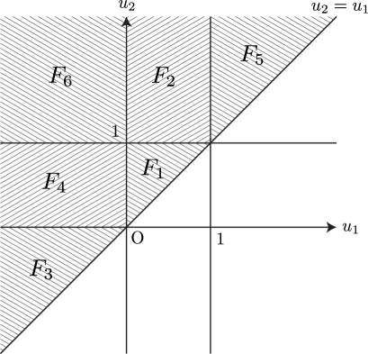
Figure 1: The six connected components of the domain of the parameters $(u_{1},u_{2})$. Added the mark $F_{i}$ to show corresponding areas to the integrals $F_{i}(q)$ to the figure of the 12 connected components given in [10].

The six components of the integration region cover the domain $u_{2}\geq u_{1}$ in the $u_{1}u_{2}$-plane. The other six components given by the exchange of 1 and 2 fill the remaining region. These 12 components of the domain in the $u_{1}u_{2}$-plane are the same as ones given in [10] to describe the domain of parameters of five-point cross-ratios. The parameters $u_{1}$, $u_{2}$ correspond to $s$, $t$ in [10]. Here, we summarize the relationship between the integrals $F_{i}(q)$ and the six components in Fig. 1.

2.2 Singularities for $F_{i}(q)$

It is convenient to express $F_{1}(q)$ in terms of the different variables $x$, $y$ given by

$$u_{1}=xy,~{}~{}~{}u_{2}=x.$$ (2.16)

$x$, $y$ also are cross-ratios:

$$x=\frac{y_{02}y_{34}}{y_{03}y_{24}},~{}~{}~{}y=\frac{y_{24}y_{01}}{y_{14}y_{02}}.$$ (2.17)

The integration region of $x$, $y$ is on the unit square $0\leq x,\,y\leq 1$ and then $F_{1}$ becomes

$$F_{1}(q) =\int^{1}_{0}dx\int^{1}_{0}dy\,\frac{-i\alpha^{\prime}}{\pi}\Big{(}\frac{q}{2}+\frac{p_{1}^{0}}{xy}+\frac{p_{2}^{0}}{x}+p_{3}^{0}\Big{)}$$

$$\quad\times x^{2\alpha^{\prime}p_{3}\cdot p_{4}-\alpha^{\prime}p_{0}\cdot p_{0}+1}(1-x)^{2\alpha^{\prime}p_{2}\cdot p_{3}}y^{2\alpha^{\prime}p_{0}\cdot p_{1}}(1-y)^{2\alpha^{\prime}p_{1}\cdot p_{2}}(1-xy)^{2\alpha^{\prime}p_{1}\cdot p_{3}},$$ (2.18)

where we have used momentum conservation and on-shell conditions.

To extract the singularity of $F_{1}(q)$ at $q=0$, we have to know the detail of the boundary of the moduli space associated with (2.18). The moduli space of a five-point tree amplitude of bosonic open strings is known as ${\cal D}_{0,5}$, which parametrizes five cyclically ordered points $y_{0},y_{1},\cdots,y_{4}$ on the boundary of the upper-half plane modulo $PSL(2,\mathbb{R})$ and has real dimension two. ${\cal D}_{0,5}$ has five boundary components ${\cal B}_{i,i+1}\ (i=0,1,\cdots,4)$[5], which parameterize limiting configurations arising from the coincidence of $y_{i}$ and $y_{i+1}$ (we identify $y_{5}$ as $y_{0}$).

From (2.17), we find that $x=0$ leads to $y_{02}=0$ or $y_{34}=0$. If $y_{02}$ becomes zero for the order $[0,1,2,3,4]$, $y_{0}$, $y_{1}$ and $y_{2}$ become coincident because $y_{1}$ is the intermediate point between $y_{0}$ and $y_{2}$. This is equivalent to $y_{34}\rightarrow 0$ up to $PSL(2,\mathbb{R})$ transformation[5] as illustrated as follows: Suppose that $y_{0}=y_{1}-h,~{}y_{2}=y_{1}+h~{}(h>0)$, $y_{0}$, $y_{1}$ and $y_{2}$ are mapped to $y_{0}^{\prime}=1$, $y_{1}^{\prime}=\infty$ and $y_{2}^{\prime}=-1$ by the $PSL(2,\mathbb{R})$ transformation

$$z^{\prime}=f(z)=\frac{-h}{z-y_{1}}.$$ (2.19)

Then, we find

$$y_{4}^{\prime}-y_{3}^{\prime}=f(y_{4})-f(y_{3})=-h\,\frac{y_{34}}{y_{13}y_{14}}.$$ (2.20)

From (2.20), as $y_{0}$, $y_{1}$ and $y_{2}$ becoming coincident ($h\rightarrow 0$), $y^{\prime}_{3}$ and $y_{4}^{\prime}$ are approaching each other in the mapped plane, while $y^{\prime}_{0}$, $y^{\prime}_{1}$ and $y^{\prime}_{2}$ are fixed.

As a result, in either case ($y_{02}=0$ or $y_{34}=0$), the limit $x\rightarrow 0$ corresponds to the boundary ${\cal B}_{34}$, and then ${\cal B}_{34}$ is parameterized by $y$. Similarly, from (2.17), we find that ${\cal B}_{01}$ is given by the limit $y\rightarrow 0$ and it is parameterized by $x$.

Noting that $q$ becomes zero for the non-zero result of ${\cal F}(q)$ (2.6), we find that in (2.18), the limits $x\rightarrow 0$ and $y\rightarrow 0$, namely ${\cal B}_{34}$ and ${\cal B}_{01}$, generate poles associated with $p_{3}\cdot p_{4}$ and $p_{0}\cdot p_{1}$, respectively. Then, it might be expected from the exponents of the integrand of (2.18) that the limits $x\rightarrow 1$ and $y\rightarrow 1$ describe ${\cal B}_{23}$ and ${\cal B}_{12}$. However, it is not the case, as seen as follows. From (2.17), we obtain

$$1-x=\frac{y_{04}y_{23}}{y_{03}y_{24}},~{}~{}~{}1-y=\frac{y_{04}y_{12}}{y_{14}y_{02}}.$$ (2.21)

So $x=1$ implies $y_{04}=0$ or $y_{23}=0$. In the order $[0,1,2,3,4]$, $(y_{0},y_{4})$ and $(y_{2},y_{3})$ are pairs of adjacent points and so $y_{04}=0$ and $y_{23}=0$ represent ${\cal B}_{40}$ and ${\cal B}_{23}$, respectively. Then it is impossible to determine uniquely the boundary represented by the limit $x\rightarrow 1$. Similarly, the limit $y\rightarrow 1$ corresponds to both boundaries, ${\cal B}_{40}$ and ${\cal B}_{12}$. As a result, $(x,y)$ is not a good coordinate in the neighborhood of the boundaries ${\cal B}_{23}$, ${\cal B}_{40}$ and ${\cal B}_{12}$.

To describe these boundaries, we transform $(x,y)$ to $(x^{\prime},y^{\prime})$ with

$$x^{\prime}=\frac{1-x}{1-xy},~{}~{}~{}y^{\prime}=1-xy.$$ (2.22)

It maps the unit square $0\leq x,\,y\leq 1$ to the unit square $0\leq x^{\prime},\,y^{\prime}\leq 1$, and $(x^{\prime},y^{\prime})$ is given by the cross-ratios:

$$x^{\prime}=\frac{y_{14}y_{23}}{y_{24}y_{13}},~{}~{}~{}y^{\prime}=\frac{y_{13}y_{04}}{y_{03}y_{14}}.$$ (2.23)

According to the above discussion, from (2.23), one can easily see that the limits $x^{\prime}\rightarrow 0$ and $y^{\prime}\rightarrow 0$ correspond to ${\cal B}_{23}$ and ${\cal B}_{40}$, respectively. For the remained boundary ${\cal B}_{12}$, we apply the same transformation as (2.22) for $(x^{\prime},y^{\prime})$:

$$x^{\prime\prime}=\frac{1-x^{\prime}}{1-x^{\prime}y^{\prime}},~{}~{}~{}y^{\prime\prime}=1-x^{\prime}y^{\prime}.$$ (2.24)

Again, $(x^{\prime\prime},y^{\prime\prime})$ is a point in the unit square. $x^{\prime\prime}$ is also the cross-ratio,

$$x^{\prime\prime}=\frac{y_{03}y_{12}}{y_{02}y_{13}},$$ (2.25)

and we find $y^{\prime\prime}=x$. From (2.25), it is clear that ${\cal B}_{12}$ is given by the limit $x^{\prime\prime}\rightarrow 0$.

By using (2.22) and (2.24), we have the five cross-ratios, $x$, $y$, $x^{\prime}$, $y^{\prime}$ and $x^{\prime\prime}$. These correspond to five-point cross-ratios used in [10] to construct the contour integral representation for the dual five-point function. As in [5], the moduli space ${\cal D}_{0,5}$ can be depicted as a pentagon, and its five boundary components correspond to ${\cal B}_{i,i+1}$. Finally, we summarize these results about the boundaries in Fig. 2.

Figure 2: The moduli space of five-point open string amplitudes corresponding to the order $[0,1,2,3,4]$. Added the limits describing the boundaries to the pentagon depicted in [5].

Let us clarify the correspondence between the pentagon and the triangle for $F_{1}(q)$. By using (2.16), (2.22) and (2.24), $(u_{1},u_{2})$ can be written by the five-point cross-ratios:

$$(u_{1},\,u_{2})=(xy,\,x)=(1-y^{\prime},\,1-x^{\prime}y^{\prime})=\left(\frac{y^{\prime\prime}(1-x^{\prime\prime})}{1-x^{\prime\prime}y^{\prime\prime}},\,y^{\prime\prime}\right).$$ (2.26)

Therefore, we find the relation between the boundaries ${\cal B}_{i,i+1}$ and parts of the triangle. As shown in Fig. 3, the boundaries ${\cal B}_{34}$ and ${\cal B}_{40}$ shrink to the points: $(0,0)$ and $(1,1)$ in the $u_{1}u_{2}$-plane.

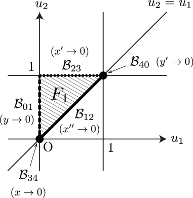
Figure 3: The correspondence of the integration domain and the moduli space for $F_{1}(q)$.

By using (2.26), we change the variables in (2.18), and then $F_{1}(q)$ is expressed in terms of $x^{\prime}$ and $y^{\prime}$ as

$$F_{1}(q) =\int_{0}^{1}dx^{\prime}\int_{0}^{1}dy^{\prime}\frac{-i\alpha^{\prime}}{\pi}\,\Big{(}\frac{q}{2}+p_{3}^{0}+p_{1}^{0}\frac{1}{1-y^{\prime}}+p_{2}^{0}\frac{1}{1-x^{\prime}y^{\prime}}\Big{)}$$

$$\quad\times{x^{\prime}}^{2\alpha^{\prime}p_{2}\cdot p_{3}}(1-x^{\prime})^{2\alpha^{\prime}p_{1}\cdot p_{2}}$$

$$\quad\times{y^{\prime}}^{2\alpha^{\prime}p_{0}\cdot p_{4}+\alpha^{\prime}p_{0}\cdot p_{0}-1}(1-y^{\prime})^{2\alpha^{\prime}p_{0}\cdot p_{1}}(1-x^{\prime}y^{\prime})^{2\alpha^{\prime}p_{0}\cdot p_{2}},$$ (2.27)

and in terms of $x^{\prime\prime}$ and $y^{\prime\prime}$ as

$$F_{1}(q) =\int_{0}^{1}dx^{\prime\prime}\int_{0}^{1}dy^{\prime\prime}\frac{-i\alpha^{\prime}}{\pi}\Big{(}\frac{q}{2}+p_{3}^{0}+p_{1}^{0}\frac{1-x^{\prime\prime}y^{\prime\prime}}{(1-x^{\prime\prime})y^{\prime\prime}}+p_{2}^{0}\frac{1}{y^{\prime\prime}}\Big{)}$$

$$\quad\times{x^{\prime\prime}}^{2\alpha^{\prime}p_{1}\cdot p_{2}}(1-x^{\prime\prime})^{2\alpha^{\prime}p_{0}\cdot p_{1}}$$

$$\quad\times{y^{\prime\prime}}^{2\alpha^{\prime}p_{3}\cdot p_{4}-\alpha^{\prime}p_{0}\cdot p_{0}+1}(1-y^{\prime\prime})^{2\alpha^{\prime}p_{0}\cdot p_{4}+\alpha^{\prime}p_{0}\cdot p_{0}-1}(1-x^{\prime\prime}y^{\prime\prime})^{2\alpha^{\prime}p_{1}\cdot p_{4}}.$$ (2.28)

Now that the coordinates describing the neighborhood of all boundaries of ${\cal D}_{0,5}$ are given, let us evaluate the singularity of $F_{1}(q)$ at $q=0$. From (2.18), (2.27) and (2.28), it turns out that the boundaries associated with $y_{0}$, which are ${\cal B}_{01}$ and ${\cal B}_{40}$, generate the delta function with respect to $q$. For ${\cal B}_{01}$, we expand the integrand of (2.18) around $y=0$ as follows:

$$F_{1}(q) =\int^{1}_{0}dx\int^{1}_{0}dy\,\frac{-i\alpha^{\prime}}{\pi}\,y^{2\alpha^{\prime}p_{0}\cdot p_{1}-1}\Big{\{}p_{1}^{0}\,x^{2\alpha^{\prime}p_{3}\cdot p_{4}-\alpha^{\prime}p_{0}\cdot p_{0}}(1-x)^{2\alpha^{\prime}p_{2}\cdot p_{3}}+{\mathrm{O}}(y)\Big{\}}.$$ (2.29)

By the Feynman $i\varepsilon$ prescription, we extract the singularity given by a neighborhood of $y=0$ [5]:

$$\int^{1}_{0}dyy^{2\alpha^{\prime}p_{0}\cdot p_{1}-1}\sim\frac{1}{-2\alpha^{\prime}qp_{1}^{0}-i\varepsilon}\sim\frac{\pi i}{2\alpha^{\prime}|p_{1}^{0}|}\delta(q),$$ (2.30)

where $\sim$ stands for equal up to terms for $q\neq 0$, which should be vanished by the BRST symmetry as seen in (2.6). Similarly, we can evaluate the singularity associated with ${\cal B}_{40}$ ($y^{\prime}\to 0$) in terms of (2.27). Finally, the singularity of $F_{1}(q)$ is given by

$$F_{1}(q) \sim\frac{1}{2}\left(\frac{p_{1}^{0}}{|p_{1}^{0}|}-\frac{p_{4}^{0}}{|p_{4}^{0}|}\right)\delta(q)I(u,s),$$ (2.31)

where we introduce the Mandelstam variables as

$$s=-(p_{1}+p_{2})^{2},~{}~{}~{}t=-(p_{1}+p_{3})^{2},~{}~{}~{}u=-(p_{1}+p_{4})^{2},$$ (2.32)

and $I(u,s)$ is defined by using the Euler beta function $B(a,b)$:

$$I(u,s) \equiv B(-\alpha^{\prime}u-1,\,-\alpha^{\prime}s-1),$$

$$B(a,b) =\int_{0}^{1}dx\,x^{a-1}(1-x)^{b-1}.$$ (2.33)

To evaluate the singularity at $q=0$ for other $F_{i}(q)\ (i=2,\cdots,6)$, in a similar way for $F_{1}(q)$, we change the variables $u_{1}$, $u_{2}$ by appropriate coordinates describing the boundary of the moduli space. The details of the calculation are shown in appendix A. Finally, we obtain the singularities of $F_{i}(q)$,

$$F_{2}(q) \sim\frac{1}{2}\left(\frac{p_{1}^{0}}{|p_{1}^{0}|}-\frac{p_{4}^{0}}{|p_{4}^{0}|}\right)\delta(q)I(t,u),$$ (2.34)

$$F_{3}(q) \sim\frac{1}{2}\left(\frac{p_{3}^{0}}{|p_{3}^{0}|}-\frac{p_{2}^{0}}{|p_{2}^{0}|}\right)\delta(q)I(u,s),$$ (2.35)

$$F_{4}(q) \sim\frac{1}{2}\left(\frac{p_{2}^{0}}{|p_{2}^{0}|}-\frac{p_{1}^{0}}{|p_{1}^{0}|}\right)\delta(q)I(u,s),$$ (2.36)

$$F_{5}(q) \sim\frac{1}{2}\left(\frac{p_{3}^{0}}{|p_{3}^{0}|}-\frac{p_{4}^{0}}{|p_{4}^{0}|}\right)\delta(q)I(s,t),$$ (2.37)

$$F_{6}(q) \sim\frac{1}{2}\left(\frac{p_{3}^{0}}{|p_{3}^{0}|}-\frac{p_{1}^{0}}{|p_{1}^{0}|}\right)\delta(q)I(t,u).$$ (2.38)

2.3 Veneziano amplitude

Now we have evaluated the singularities at $q=0$ of all $F_{i}(q)$, namely those of ${\cal F}(q)$ given by (2.14). Noting that ${\cal F}(q)\ (q\neq 0)$ has no contribution to the amplitude as mentioned in (2.6), we can calculate the amplitude (2.3) by using (2.14) and by adding together (2.31), (2.34), (2.35), (2.36), (2.37) and (2.38). The resulting amplitude is

$${\cal A}_{4} =\frac{1}{2}\Big{(}\frac{p_{3}^{0}}{|p_{3}^{0}|}-\frac{p_{4}^{0}}{|p_{4}^{0}|}\Big{)}\times A_{4},$$ (2.39)

where $A_{4}$ is the Veneziano amplitude, which is same as (6.4.9) in [11]:

$$A_{4}=2ig_{\rm o}^{4}C_{D_{2}}(2\pi)^{26}\delta^{26}\big{(}\sum_{k=1}^{4}p_{k}\big{)}\,(I(s,t)+I(t,u)+I(u,s)).$$ (2.40)

Thus, we have derived the Veneziano amplitude from the five-point function where one of the vertices is the mostly BRST exact operator.

We should comment that the sign factor in (2.39) is interpreted as the signed intersection number as discussed in [3]. The mostly BRST exact operator is constructed by the gauge fixing condition $X^{0}(y_{0})=0$, and then the Faddev-Popov determinant for the gauge fixing includes $\partial X^{0}(y_{0})$. The important point is that we do not take the absolute value of the determinant as a conventional operator formalism. Moreover, the fixed operators at $y_{3}$ and $y_{4}$ correspond to asymptotic states in the scattering process, and so the time coordinates $X^{0}(y_{3})$ and $X^{0}(y_{4})$ become $-\infty$ or $+\infty$ depending on whether the state is incoming or outgoing. Consequently, the sign of the amplitude is given as the signed intersection number of the graph $u=X^{0}(y)$ with $u=0$, and this is determined by whether the fixed vertices are incoming or outgoing. It is easily seen that the sign does not depend on the momenta of the integrated vertices. As a result, the sign factor of (2.39) is in agreement with that of the three-point amplitude in [3] derived from the four-point function with ${\mathpzc E}$.

3 Concluding remarks

We have shown that the five-point function for four open string tachyon vertices and the mostly BRST exact operator ${\mathpzc E}$ coincides with the Veneziano amplitude up to the sign factor, which depends on the external momenta and takes the value, $\pm 1$ or 0. In the calculation, the contribution from the singularity near the boundary of the moduli space was significant. We have used the Feynman $i\varepsilon$ prescription to extract the singularities after [3].

The result of amplitudes with the insertion of ${\mathpzc E}$ is represented by the following equation:

$$ig_{\rm o}^{n}C_{D_{2}}\!\left<0\right|{\mathpzc E}(y_{0})\int_{-\infty}^{\infty}dy_{1}V_{1}(y_{1})\cdots\int_{-\infty}^{\infty}dy_{n-2}V_{n-2}(y_{n-2})\,cV_{n-1}(y_{n-1})\,cV_{n}(y_{n})\left|0\right>\!$$

$$=\frac{1}{2}\Big{(}\frac{p_{n-1}^{0}}{|p_{n-1}^{0}|}-\frac{p_{n}^{0}}{|p_{n}^{0}|}\Big{)}\times A_{n},$$ (3.1)

where $A_{n}$ is the correct $n$-point open string amplitude for the vertices $V_{i}(y_{i})\ (i=1,\cdots,n)$. For $n=2$, this is shown in [2] as two-point amplitudes for arbitrary vertices. For $n=3$, this is given in [3] for tachyon vertex operators. Then, in the case of $n=4$ for tachyon vertices, $A_{n}$ is the Veneziano amplitude, and this is proven in this paper. For tachyon vertices, $A_{n}\ (n\geq 5)$ is given by the Koba-Nielsen amplitude and the sign factor is expected to be the same as $n=2,3,4$ from the interpretation of the signed intersection number. The equation (3.1) is conjectured to hold in this general case $(n\geq 5)$.

We expect that similar identities hold for arbitrary vertex operators. In fact, for $n=2$, (3.1) is true for arbitrary external states[2, 3]. To prove these, it is necessary to understand the moduli space for corresponding amplitudes similarly to the derivation of the Veneziano amplitude from the five-point function.

Appendix A Evaluation of $F_{i}(q)~{}~{}~{}(i=2,\cdots,6)$

A.1 $F_{2}(q)$

According to Fig. 1, the integral $F_{2}(q)$ is given by the form

$$F_{2}(q) =\int_{1}^{\infty}du_{2}\int_{0}^{1}du_{1}\cdots.$$ (A.1)

By changing the variables, $u_{1}=y$, $u_{2}=1/x$, we can express $F_{2}(q)$ as the integral over the unit square:

$$F_{2}(q) =\int_{0}^{1}dx\int_{0}^{1}dy\frac{-i\alpha^{\prime}}{\pi}\Big{(}\frac{q}{2}+p^{0}_{3}+p_{1}^{0}\frac{1}{y}+p_{2}^{0}\,x\Big{)}$$

$$\quad\times x^{2\alpha^{\prime}p_{2}\cdot p_{4}}(1-x)^{2\alpha^{\prime}p_{2}\cdot p_{3}}y^{2\alpha^{\prime}p_{0}\cdot p_{1}}(1-y)^{2\alpha^{\prime}p_{1}\cdot p_{3}}(1-xy)^{2\alpha^{\prime}p_{1}\cdot p_{2}}.$$ (A.2)

By the transformations (2.22) and (2.24) for $(x,y)$, we can obtain different expressions for $F_{2}(q)$:

$$F_{2}(q) =\int_{0}^{1}dx^{\prime}\int_{0}^{1}dy^{\prime}\frac{-i\alpha^{\prime}}{\pi}\Big{(}\frac{q}{2}+p^{0}_{3}+p^{0}_{1}\,\frac{1-x^{\prime}y^{\prime}}{1-y^{\prime}}+p^{0}_{2}\,(1-x^{\prime}y^{\prime})\Big{)}$$

$$\quad\times{x^{\prime}}^{2\alpha^{\prime}p_{2}\cdot p_{3}}(1-x^{\prime})^{2\alpha^{\prime}p_{1}\cdot p_{3}}{y^{\prime}}^{2\alpha^{\prime}p_{0}\cdot p_{4}+\alpha^{\prime}p_{0}\cdot p_{0}-1}(1-y^{\prime})^{2\alpha^{\prime}p_{0}\cdot p_{1}}(1-x^{\prime}y^{\prime})^{2\alpha^{\prime}p_{0}\cdot p_{3}+\alpha^{\prime}p_{0}\cdot p_{0}-1}$$ (A.3)

$$=\int_{0}^{1}dx^{\prime\prime}\int_{0}^{1}dy^{\prime\prime}\frac{-i\alpha^{\prime}}{\pi}\Big{(}\frac{q}{2}+p^{0}_{3}+p^{0}_{1}\,\frac{1-x^{\prime\prime}y^{\prime\prime}}{1-x^{\prime\prime}}+p^{0}_{2}\,y^{\prime\prime}\Big{)}$$

$$\quad\times{x^{\prime\prime}}^{2\alpha^{\prime}p_{1}\cdot p_{3}}(1-x^{\prime\prime})^{2\alpha^{\prime}p_{1}\cdot p_{0}}{y^{\prime\prime}}^{2\alpha^{\prime}p_{2}\cdot p_{4}}(1-y^{\prime\prime})^{2\alpha^{\prime}p_{0}\cdot p_{4}+\alpha^{\prime}p_{0}\cdot p_{0}-1}(1-x^{\prime\prime}y^{\prime\prime})^{2\alpha^{\prime}p_{1}\cdot p_{4}}.$$ (A.4)

Since $u_{1}$ and $u_{2}$ are given by (2.7), the five-point cross-ratios for $F_{2}(q)$ are explicitly written as

$$x=\dfrac{y_{03}y_{24}}{y_{02}y_{34}},\quad y=\dfrac{y_{01}y_{34}}{y_{03}y_{14}},\quad x^{\prime}=-\dfrac{y_{14}y_{23}}{y_{12}y_{34}},\quad y^{\prime}=\dfrac{y_{04}y_{12}}{y_{02}y_{14}},\quad x^{\prime\prime}=\dfrac{y_{02}y_{13}}{y_{03}y_{12}}.$$ (A.5)

From these expressions, we determine the limits corresponding to the boundaries of the moduli space for the order $[0,1,3,2,4]$:

$${\cal B}_{24}:(x\to 0), {\cal B}_{01}:(y\to 0), {\cal B}_{32}:(x^{\prime}\to 0), {\cal B}_{40}:(y^{\prime}\to 0), {\cal B}_{13}:(x^{\prime\prime}\to 0).$$ (A.6)

The original parameters $u_{1}$ and $u_{2}$ are written using the five-point cross-ratios such as

$$(u_{1},\,u_{2})=\Big{(}y,\,\frac{1}{x}\Big{)}=\left(\frac{1-y^{\prime}}{1-x^{\prime}y^{\prime}},\frac{1}{1-x^{\prime}y^{\prime}}\right)=\left(\frac{1-x^{\prime\prime}}{1-x^{\prime\prime}y^{\prime\prime}},\frac{1}{y^{\prime\prime}}\right).$$ (A.7)

Therefore we depict the domain for $F_{2}(q)$ and the boundaries of the moduli space as in Fig. 4. We find that ${\cal B}_{40}$ shrinks to a point in the $u_{1}u_{2}$-plane.

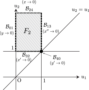
Figure 4: The correspondence of the integration domain and the moduli space for $F_{2}(q)$.

Now let us evaluate the singularity of $F_{2}(q)$, which arises from the boundaries ${\cal B}_{01}$ and ${\cal B}_{40}$. Similar to the case of $F_{1}(q)$, we expand the integrand of (A.2) around $y=0$ for ${\cal B}_{01}$ and that of (A.3) around $y^{\prime}=0$ for ${\cal B}_{40}$. Then we extract the delta function of $q$ by using the $i\varepsilon$ prescription. We obtain the resulting expression for $F_{2}(q)$ in (2.34).

A.2 $F_{3}(q)$

For the order $[1,2,0,3,4]$, from Fig. 1, it turns out that the integral $F_{3}(q)$ is written as

$$F_{3}(q) =\int_{-\infty}^{0}du_{2}\int_{-\infty}^{u_{2}}du_{1}\cdots.$$ (A.8)

We change the variables by a $PSL(2,\mathbb{R})$ transformation:

$$u^{\prime}_{1}=\frac{1}{1-u_{1}},\quad u^{\prime}_{2}=\frac{1}{1-u_{2}},$$ (A.9)

to map the integration region onto the triangle domain as $F_{1}(q)$. Then $F_{3}(q)$ is expressed as

$$F_{3}(q) =\int_{0}^{1}du_{2}^{\prime}\int_{0}^{u_{2}^{\prime}}du_{1}^{\prime}\frac{1}{(u_{1}^{\prime}u_{2}^{\prime})^{2}}\cdots.$$ (A.10)

Since the integration range of $F_{3}(q)$ becomes equal to that of $F_{1}(q)$, we follow the same procedure applied to evaluate the singularity of $F_{1}(q)$. Using $u_{1}^{\prime}=xy$ and $u_{2}^{\prime}=x$, we change the coordinates by (2.22) and (2.24), and we have the five-point cross-ratios:

$$x=\dfrac{y_{03}y_{24}}{y_{23}y_{04}}, y=\dfrac{y_{23}y_{14}}{y_{13}y_{24}}, x^{\prime}=\dfrac{y_{13}y_{02}}{y_{01}y_{23}}, y^{\prime}=-\dfrac{y_{01}y_{34}}{y_{04}y_{13}}, x^{\prime\prime}=-\dfrac{y_{12}y_{04}}{y_{01}y_{24}}.$$ (A.11)

The boundaries of the moduli space are given by the limits:

$${\cal B}_{03}:(x\to 0), {\cal B}_{41}:(y\to 0), {\cal B}_{20}:(x^{\prime}\to 0), {\cal B}_{34}:(y^{\prime}\to 0), {\cal B}_{12}:(x^{\prime\prime}\to 0).$$ (A.12)

$u_{1}$ and $u_{2}$ are expressed by the five-point cross-ratios as

$$(u_{1},\,u_{2})=\left(\frac{xy-1}{xy},\,\frac{x-1}{x}\right)=\left(\frac{y^{\prime}}{y^{\prime}-1},\,\frac{x^{\prime}y^{\prime}}{x^{\prime}y^{\prime}-1}\right)=\left(\frac{y^{\prime\prime}-1}{y^{\prime\prime}(1-x^{\prime\prime})},\,\frac{y^{\prime\prime}-1}{y^{\prime\prime}}\right).$$ (A.13)

So we summarize the domain for $F_{3}(q)$ in the $u_{1}u_{2}$-plane in Fig. 5.

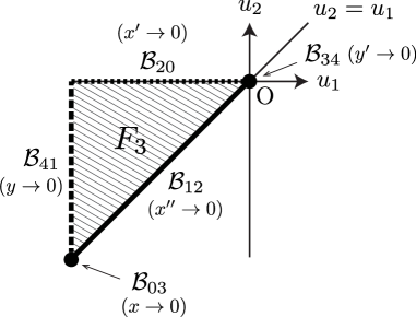
Figure 5: The correspondence of the integration domain and the moduli space for $F_{3}(q)$.

By using the five-point cross-ratios, $F_{3}(q)$ can be written as

$$F_{3}(q) =\int_{0}^{1}dx\int_{0}^{1}dy\frac{-i\alpha^{\prime}}{\pi}\Big{(}\frac{q}{2}+p^{0}_{3}+p_{1}^{0}\,\frac{xy}{xy-1}+p^{0}_{2}\frac{x}{x-1}\Big{)}$$

$$\quad\times x^{2\alpha^{\prime}p_{0}\cdot p_{3}+\alpha^{\prime}p_{0}\cdot p_{0}-1}(1-x)^{2\alpha^{\prime}p_{0}\cdot p_{2}}y^{2\alpha^{\prime}p_{1}\cdot p_{4}}(1-y)^{2\alpha^{\prime}p_{1}\cdot p_{2}}(1-xy)^{2\alpha^{\prime}p_{0}\cdot p_{1}}$$ (A.14)

$$=\int_{0}^{1}dx^{\prime}\int_{0}^{1}dy^{\prime}\frac{-i\alpha^{\prime}}{\pi}\Big{(}\frac{q}{2}+p^{0}_{3}+p^{0}_{1}\,\frac{y^{\prime}-1}{y^{\prime}}+p^{0}_{2}\frac{x^{\prime}y^{\prime}-1}{x^{\prime}y^{\prime}}\Big{)}$$

$$\quad\times{x^{\prime}}^{2\alpha^{\prime}p_{0}\cdot p_{2}}(1-x^{\prime})^{2\alpha^{\prime}p_{1}\cdot p_{2}}{y^{\prime}}^{2\alpha^{\prime}p_{3}\cdot p_{4}-\alpha^{\prime}p_{0}\cdot p_{0}+1}(1-y^{\prime})^{2\alpha^{\prime}p_{1}\cdot p_{4}}(1-x^{\prime}y^{\prime})^{2\alpha^{\prime}p_{2}\cdot p_{4}}$$ (A.15)

$$=\int_{0}^{1}dx^{\prime\prime}\int_{0}^{1}dy^{\prime\prime}\frac{-i\alpha^{\prime}}{\pi}\Big{(}\frac{q}{2}+p^{0}_{3}+p^{0}_{1}\,\frac{(1-x^{\prime\prime})y^{\prime\prime}}{y^{\prime\prime}-1}+p^{0}_{2}\,\frac{y^{\prime\prime}}{y^{\prime\prime}-1}\Big{)}$$

$$\quad\times{x^{\prime\prime}}^{2\alpha^{\prime}p_{1}\cdot p_{2}}(1-x^{\prime\prime})^{2\alpha^{\prime}p_{1}\cdot p_{4}}{y^{\prime\prime}}^{2\alpha^{\prime}p_{0}\cdot p_{3}+\alpha^{\prime}p_{0}\cdot p_{0}-1}(1-y^{\prime\prime})^{2\alpha^{\prime}p_{3}\cdot p_{4}-\alpha^{\prime}p_{0}\cdot p_{0}+1}(1-x^{\prime\prime}y^{\prime\prime})^{2\alpha^{\prime}p_{1}\cdot p_{3}}.$$

Since the boundaries ${\cal B}_{03}$ and ${\cal B}_{20}$ contribute to the singularity, we have only to expand (A.14) and (A.15) around $x=0$ and $x^{\prime}=0$, respectively. We obtain the final result for $F_{3}(q)$ as (2.35).

A.3 $F_{4}(q)$

The integration region of $F_{4}(q)$ is depicted in Fig. 1. Similar to the case of $F_{2}(q)$, we can map this region onto the unit square by

$$x=1-u_{1},\qquad y=\frac{1}{1-u_{2}}.$$ (A.17)

After that, we follow the same procedure as for $F_{1}$, $F_{2}$ and $F_{3}$. We can introduce the five-point cross-ratios using the transformations (2.22) and (2.24):

$$x=\dfrac{y_{23}y_{04}}{y_{03}y_{24}}, y=\dfrac{y_{03}y_{14}}{y_{13}y_{04}}, x^{\prime}=\dfrac{y_{02}y_{13}}{y_{03}y_{12}}, y^{\prime}=\dfrac{y_{12}y_{34}}{y_{24}y_{13}}, x^{\prime\prime}=-\dfrac{y_{01}y_{24}}{y_{04}y_{12}}.$$ (A.18)

So the five boundaries of the moduli space are given by the limits:

$${\cal B}_{23}:(x\to 0), {\cal B}_{41}:(y\to 0), {\cal B}_{02}:(x^{\prime}\to 0), {\cal B}_{34}:(y^{\prime}\to 0), {\cal B}_{10}:(x^{\prime\prime}\to 0).$$ (A.19)

Then $(u_{1},u_{2})$ is written by

$$(u_{1},\,u_{2})=\left(\frac{y-1}{y},1-x\right)=\left(\frac{y^{\prime}(1-x^{\prime})}{y^{\prime}-1},\,x^{\prime}y^{\prime}\right)=\left(\frac{x^{\prime\prime}(1-y^{\prime\prime})}{x^{\prime\prime}-1},\,1-y^{\prime\prime}\right).$$ (A.20)

The domain for $F_{4}(q)$ and the boundaries in the $u_{1}u_{2}$-plane are shown in Fig. 6.

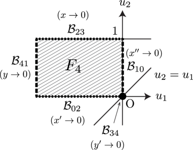
Figure 6: The correspondence of the integration domain and the moduli space for $F_{4}(q)$.

By the transformations (A.20), $F_{4}(q)$ can be expressed as

$$F_{4}(q) =\int_{0}^{1}dx\int_{0}^{1}dy\frac{-i\alpha}{\pi}\Big{(}\frac{q}{2}+p^{0}_{3}+p^{0}_{1}\,\frac{y}{y-1}+p^{0}_{2}\frac{1}{1-x}\Big{)}$$

$$\quad\times x^{2\alpha^{\prime}p_{2}\cdot p_{3}}(1-x)^{2\alpha^{\prime}p_{0}\cdot p_{2}}y^{2\alpha^{\prime}p_{1}\cdot p_{4}}(1-y)^{2\alpha^{\prime}p_{0}\cdot p_{1}}(1-xy)^{2\alpha^{\prime}p_{1}\cdot p_{2}}$$ (A.21)

$$=\int_{0}^{1}dx^{\prime}\int_{0}^{1}dy^{\prime}\frac{-i\alpha^{\prime}}{\pi}\Big{(}\frac{q}{2}+p^{0}_{3}+p^{0}_{1}\frac{y^{\prime}-1}{(1-x^{\prime})y^{\prime}}+p^{0}_{2}\frac{1}{x^{\prime}y^{\prime}}\Big{)}$$

$$\quad\times{x^{\prime}}^{2\alpha^{\prime}p_{0}\cdot p_{2}}(1-x^{\prime})^{2\alpha^{\prime}p_{0}\cdot p_{1}}{y^{\prime}}^{2\alpha^{\prime}p_{3}\cdot p_{4}-\alpha^{\prime}p_{0}\cdot p_{0}+1}(1-y^{\prime})^{2\alpha^{\prime}p_{1}\cdot p_{4}}(1-x^{\prime}y^{\prime})^{2\alpha^{\prime}p_{0}\cdot p_{4}+\alpha^{\prime}p_{0}\cdot p_{0}-1}$$ (A.22)

$$=\int_{0}^{1}dx^{\prime\prime}\int_{0}^{1}dy^{\prime\prime}\frac{-i\alpha^{\prime}}{\pi}\Big{(}\frac{q}{2}+p^{0}_{3}+p^{0}_{1}\frac{x^{\prime\prime}-1}{x^{\prime\prime}(1-y^{\prime\prime})}+p^{0}_{2}\frac{1}{1-y^{\prime\prime}}\Big{)}$$

$$\quad\times{x^{\prime\prime}}^{2\alpha^{\prime}p_{0}\cdot p_{1}}(1-x^{\prime\prime})^{2\alpha^{\prime}p_{1}\cdot p_{4}}{y^{\prime\prime}}^{2\alpha^{\prime}p_{2}\cdot p_{3}}(1-y^{\prime\prime})^{2\alpha^{\prime}p_{3}\cdot p_{4}-\alpha^{\prime}p_{0}\cdot p_{0}+1}(1-x^{\prime\prime}y^{\prime\prime})^{2\alpha^{\prime}p_{1}\cdot p_{3}}.$$ (A.23)

To extract the singularity, we expand the integrand of $F_{4}(q)$ around $x^{\prime}=0$ for ${\cal B}_{02}$ and $x^{\prime\prime}=0$ for ${\cal B}_{10}$. The resulting expression for $F_{4}(q)$ becomes (2.36).

A.4 $F_{5}(q)$

As for $F_{5}(q)$, we can map the integration region in Fig. 1 onto the triangle for $F_{1}(q)$ by a $PSL(2,\mathbb{R})$ transformation:

$$u_{1}^{\prime\prime}=\frac{u_{1}-1}{u_{1}},\qquad u_{2}^{\prime\prime}=\frac{u_{2}-1}{u_{2}}.$$ (A.24)

With $u_{1}^{\prime\prime}=xy$ and $u_{2}^{\prime\prime}=x$, the five-point cross-ratios are introduced by (2.22) and (2.24):

$$x=-\dfrac{y_{04}y_{23}}{y_{02}y_{34}}, y=\dfrac{y_{02}y_{13}}{y_{01}y_{23}}, x^{\prime}=\dfrac{y_{01}y_{24}}{y_{02}y_{14}}, y^{\prime}=\dfrac{y_{03}y_{14}}{y_{01}y_{34}}, x^{\prime\prime}=-\dfrac{y_{12}y_{34}}{y_{23}y_{14}}.$$ (A.25)

Therefore, the boundaries of the moduli space are given by

$${\cal B}_{40}:(x\to 0), {\cal B}_{31}:(y\to 0), {\cal B}_{24}:(x^{\prime}\to 0), {\cal B}_{03}:(y^{\prime}\to 0), {\cal B}_{12}:(x^{\prime\prime}\to 0).$$ (A.26)

$(u_{1},u_{2})$ is expressed as

$$(u_{1},\,u_{2})=\left(\frac{1}{1-xy},\frac{1}{1-x}\right)=\left(\frac{1}{y^{\prime}},\,\frac{1}{x^{\prime}y^{\prime}}\right)=\left(\frac{1-x^{\prime\prime}y^{\prime\prime}}{1-y^{\prime\prime}},\,\frac{1}{1-y^{\prime\prime}}\right),$$ (A.27)

and the domain and boundaries for $F_{5}(q)$ in the $u_{1}u_{2}$-plane are summarized in Fig. 7.

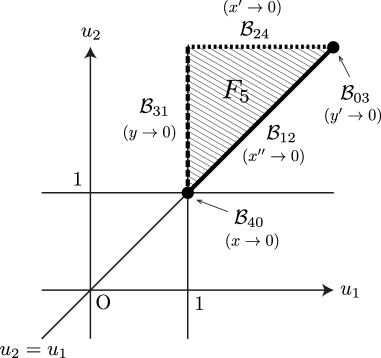
Figure 7: The correspondence of the integration domain and the moduli space for $F_{5}(q)$.

Using the above results, we can express $F_{5}(q)$ in terms of the five-point cross-ratios:

$$F_{5}(q) =\int_{0}^{1}dx\int_{0}^{1}dy\frac{-i\alpha^{\prime}}{\pi}\Big{(}\frac{q}{2}+p^{0}_{3}+p^{0}_{1}\,(1-xy)+p^{0}_{2}\,(1-x)\Big{)}$$

$$\quad\times x^{2\alpha^{\prime}p_{0}\cdot p_{4}+\alpha^{\prime}p_{0}\cdot p_{0}-1}(1-x)^{2\alpha^{\prime}p_{2}\cdot p_{4}}y^{2\alpha^{\prime}p_{1}\cdot p_{3}}(1-y)^{2\alpha^{\prime}p_{1}\cdot p_{2}}(1-xy)^{2\alpha^{\prime}p_{1}\cdot p_{4}}$$ (A.28)

$$=\int_{0}^{1}dx^{\prime}\int_{0}^{1}dy^{\prime}\frac{-i\alpha^{\prime}}{\pi}\Big{(}\frac{q}{2}+p^{0}_{3}+p^{0}_{1}\,y^{\prime}+p^{0}_{2}\,x^{\prime}y^{\prime}\Big{)}\Big{)}$$

$$\quad\times{x^{\prime}}^{2\alpha^{\prime}p_{2}\cdot p_{4}}(1-x^{\prime})^{2\alpha^{\prime}p_{1}\cdot p_{2}}{y^{\prime}}^{2\alpha^{\prime}p_{0}\cdot p_{3}+\alpha^{\prime}p_{0}\cdot p_{0}-1}(1-y^{\prime})^{2\alpha^{\prime}p_{1}\cdot p_{3}}(1-x^{\prime}y^{\prime})^{2\alpha^{\prime}p_{2}\cdot p_{3}}$$ (A.29)

$$=\int_{0}^{1}dx^{\prime\prime}\int_{0}^{1}dy^{\prime\prime}\frac{-i\alpha^{\prime}}{\pi}\Big{(}\frac{q}{2}+p^{0}_{3}+p^{0}_{1}\frac{1-y^{\prime\prime}}{1-x^{\prime\prime}y^{\prime\prime}}+p^{0}_{2}\,(1-y^{\prime\prime})\Big{)}\Big{)}$$

$$\quad\times{x^{\prime\prime}}^{2\alpha^{\prime}p_{1}\cdot p_{2}}(1-x^{\prime\prime})^{2\alpha^{\prime}p_{1}\cdot p_{3}}{y^{\prime\prime}}^{2\alpha^{\prime}p_{0}\cdot p_{4}+\alpha^{\prime}p_{0}\cdot p_{0}-1}(1-y^{\prime\prime})^{2\alpha^{\prime}p_{0}\cdot p_{3}+\alpha^{\prime}p_{0}\cdot p_{0}-1}(1-x^{\prime\prime}y^{\prime\prime})^{2\alpha^{\prime}p_{0}\cdot p_{1}}.$$ (A.30)

We expand the integrand of $F_{5}(q)$ around the boundaries associated with the zeroth vertex (${\cal B}_{40}$ and ${\cal B}_{03}$). Then, by using the $i\varepsilon$ prescription, the singularities are extracted as (2.37).

A.5 $F_{6}(q)$

For $F_{6}(q)$, we can map the integration region in Fig. 1 onto the unit square by

$$x=\frac{u_{1}}{u_{1}-1},\qquad y=\frac{u_{2}-1}{u_{2}}.$$ (A.31)

After that, the five-point cross-ratios are introduced by (2.22) and (2.24):

$$x=-\dfrac{y_{01}y_{34}}{y_{04}y_{13}}, y=-\dfrac{y_{04}y_{23}}{y_{02}y_{34}}, x^{\prime}=\dfrac{y_{02}y_{14}}{y_{04}y_{12}}, y^{\prime}=\dfrac{y_{03}y_{12}}{y_{02}y_{13}}, x^{\prime\prime}=\dfrac{y_{13}y_{24}}{y_{12}y_{34}}.$$ (A.32)

Therefore, the boundaries of the moduli space are given by

$${\cal B}_{10}:(x\to 0), {\cal B}_{32}:(y\to 0), {\cal B}_{41}:(x^{\prime}\to 0), {\cal B}_{03}:(y^{\prime}\to 0), {\cal B}_{24}:(x^{\prime\prime}\to 0).$$ (A.33)

$(u_{1},u_{2})$ is written by

$$(u_{1},\,u_{2})=\left(\frac{x}{x-1},\frac{1}{1-y}\right)=\left(\frac{x^{\prime}y^{\prime}-1}{x^{\prime}y^{\prime}},\,\frac{1-x^{\prime}y^{\prime}}{y^{\prime}(1-x^{\prime})}\right)=\left(\frac{y^{\prime\prime}}{y^{\prime\prime}-1},\,\frac{1-x^{\prime\prime}y^{\prime\prime}}{x^{\prime\prime}(1-y^{\prime\prime})}\right),$$ (A.34)

and the domain and boundaries for $F_{6}(q)$ in the $u_{1}u_{2}$-plane are summarized in Fig. 8.

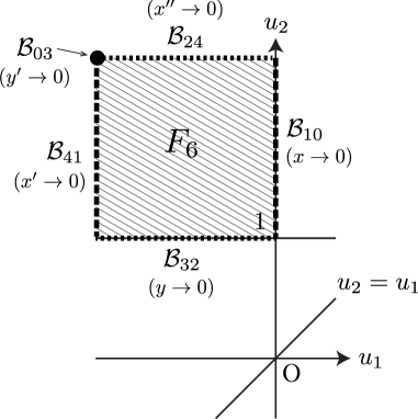
Figure 8: The correspondence of the integration domain and the moduli space for $F_{6}(q)$.

Using the above results, we can express $F_{6}(q)$ in terms of the five-point cross-ratios:

$$F_{6}(q) =\int_{0}^{1}dx\int_{0}^{1}dy\frac{-i\alpha^{\prime}}{\pi}\Big{(}\frac{q}{2}+p^{0}_{3}+p^{0}_{1}\frac{x-1}{x}+p^{0}_{2}\,(1-y)\Big{)}$$

$$\quad\times x^{2\alpha^{\prime}p_{0}\cdot p_{1}}(1-x)^{2\alpha^{\prime}p_{1}\cdot p_{4}}y^{2\alpha^{\prime}p_{2}\cdot p_{3}}(1-y)^{2\alpha^{\prime}p_{2}\cdot p_{4}}(1-xy)^{2\alpha^{\prime}p_{1}\cdot p_{2}}$$ (A.35)

$$=\int_{0}^{1}dx^{\prime}\int_{0}^{1}dy^{\prime}\frac{-i\alpha^{\prime}}{\pi}\Big{(}\frac{q}{2}+p^{0}_{3}+p^{0}_{1}\frac{x^{\prime}y^{\prime}}{x^{\prime}y^{\prime}-1}+p^{0}_{2}\,\frac{(1-x^{\prime})y^{\prime}}{1-x^{\prime}y^{\prime}}\Big{)}$$

$$\quad\times{x^{\prime}}^{2\alpha^{\prime}p_{1}\cdot p_{4}}(1-x^{\prime})^{2\alpha^{\prime}p_{2}\cdot p_{4}}{y^{\prime}}^{2\alpha^{\prime}p_{0}\cdot p_{3}+\alpha^{\prime}p_{0}\cdot p_{0}-1}(1-y^{\prime})^{2\alpha^{\prime}p_{2}\cdot p_{3}}(1-x^{\prime}y^{\prime})^{2\alpha^{\prime}p_{3}\cdot p_{4}-\alpha^{\prime}p_{0}\cdot p_{0}+1}$$ (A.36)

$$=\int_{0}^{1}dx^{\prime\prime}\int_{0}^{1}dy^{\prime\prime}\frac{-i\alpha^{\prime}}{\pi}\Big{(}\frac{q}{2}+p^{0}_{3}+p^{0}_{1}\frac{y^{\prime\prime}-1}{y^{\prime\prime}}+p^{0}_{2}\,\frac{x^{\prime\prime}(1-y^{\prime\prime})}{1-x^{\prime\prime}y^{\prime\prime}}\Big{)}$$

$$\quad\times{x^{\prime\prime}}^{2\alpha^{\prime}p_{2}\cdot p_{4}}(1-x^{\prime\prime})^{2\alpha^{\prime}p_{2}\cdot p_{3}}{y^{\prime\prime}}^{2\alpha^{\prime}p_{0}\cdot p_{1}}(1-y^{\prime\prime})^{2\alpha^{\prime}p_{0}\cdot p_{3}+\alpha^{\prime}p_{0}\cdot p_{0}-1}(1-x^{\prime\prime}y^{\prime\prime})^{2\alpha^{\prime}p_{0}\cdot p_{2}}.$$ (A.37)

We expand the integrand of $F_{6}(q)$ around the boundaries associated with the zeroth vertex (${\cal B}_{10}$ and ${\cal B}_{03}$). Then, by using the $i\varepsilon$ prescription, the singularities are given as (2.38).

References

- [1] H. Erbin, J. Maldacena and D. Skliros, “Two-Point String Amplitudes,” JHEP 07 (2019) 139 [arXiv:1906.06051 [hep-th]].
- [2] S. Seki and T. Takahashi, “Two-point String Amplitudes Revisited by Operator Formalism,” Phys. Lett. B 800 (2020) 135078 [arXiv:1909.03672 [hep-th]].
- [3] S. Seki and T. Takahashi, “Reduction of Open String Amplitudes by Mostly BRST Exact Operators,” [arXiv:2108.05628 [hep-th]].
- [4] S. P. Kashyap, “Two-Point Superstring Tree Amplitudes Using the Pure Spinor Formalism,” [arXiv:2012.03802 [hep-th]].
- [5] E. Witten, “The Feynman in String Theory,” JHEP 04 (2015) 055 [arXiv:1307.5124 [hep-th]].
- [6] G. Veneziano, “Construction of a crossing - symmetric, Regge behaved amplitude for linearly rising trajectories,” Nuovo Cim. A 57 (1968) 190-197.
- [7] K. Bardakci and H. Ruegg, “Reggeized resonance model for the production amplitude,” Phys. Lett. B 28 (1968) 342-347.
- [8] M. A. Virasoro, “Generalization of veneziano’s formula for the five-point function,” Phys. Rev. Lett. 22 (1969) 37-39.
- [9] Z. Koba and H. B. Nielsen, “Reaction amplitude for n mesons: A Generalization of the Veneziano-Bardakci-Ruegg-Virasora model,” Nucl. Phys. B 10 (1969) 633-655.
- [10] A. J. Hanson and J. Sha, “A Contour Integral Representation for the Dual Five-Point Function and a Symmetry of the Genus Four Surface in R6,” J. Phys. A: Math. Gen. 39 (2006) 2509-2537 [arXiv:math-ph/0510064].
- [11] J. Polchinski, String theory. Vol. 1: An introduction to the bosonic string, Cambridge Univ. Pr., UK, 1998.