Current-Induced Spin-Wave Doppler Shift in Antiferromagnets

Abstract

We theoretically study the spin dynamics in antiferromagnets (AFs) under the influence of an electric current. We identify two different sources of spin-transfer torques that stem from uniform (${\bm{v}}_{n}$) and staggered (${\bm{v}}_{\ell}$) electron spin densities. While the former is well recognized, the latter is often overlooked. We show that both ${\bm{v}}_{n}$ and ${\bm{v}}_{\ell}$ contribute equally to the spin-wave Doppler shift. Microscopic calculations are presented for electrons on a two-dimensional square lattice with nearest-neighbor ($t$) and next-nearest-neighbor ($t^{\prime}$) hopping, which interpolate two opposite transport regimes of strongly-coupled AF ($t^{\prime}/t\ll 1$) and two weakly-coupled ferromagnets ($t^{\prime}/t\gg 1$). In the AF transport regime ($t^{\prime}/t\ll 1$), ${\bm{v}}_{n}$ and ${\bm{v}}_{\ell}$ have opposite signs, and the sign of the Doppler shift depends on band filling; ${\bm{v}}_{n}$ (${\bm{v}}_{\ell}$) is dominant near the AF gap (near the band bottom or the top). As $t^{\prime}/t$ is increased, ${\bm{v}}_{n}$ undergoes a sign change whereas ${\bm{v}}_{\ell}$ does not. In the limit of vanishing $t$, ${\bm{v}}_{n}$ and ${\bm{v}}_{\ell}$ coincide and the spin-transfer torque reduces to that of ferromagnets.

Spin waves are low-energy excitations of magnetically ordered systems that carry heat and angular momentum, and are expected to play important roles in spintronics. Unlike electric currents that can also carry heat and angular momentum, spin waves do not suffer Joule heating and can be more energy efficient. Although much of the work done so far have focused on ferromagnets (FMs), a new surge in the interest of antiferromagnetic (AF) spintronics sheds light on new possibilities of spin waves.

Antiferromagnets (AFs) are a class of materials with many advantages over FMs, such as the absence of leakage magnetic field, rigidity to magnetic perturbations, fast spin dynamics, and diverse candidate materials [1, 2, 3, 4]. The fast spin dynamics of AFs allows for spin waves that can reach frequencies in the terahertz range, while ferromagnetic (FM) spin waves remain in the gigahertz range. AF spin waves come with another perk that might revolutionize magnonics, which is the chirality or isospin degree of freedom [5]. In contrast to FM spin waves that can only encode information in the amplitude, AF spin waves have multiple modes with different chiralities. Specifically, collinear AFs possess two degenerate eigenmodes with opposite chiralities. Despite the highly anticipated features of AF spin waves, the means to control them remain limited.

From a scalability perspective, electrical manipulation of spin waves is ideal. In FMs, the effects of electric current on spin waves are relatively well known [6, 7, 8, 9, 10]. In particular, the (reactive) spin-transfer torque (STT) causes a Doppler shift on spin waves, which can be used as a probe of spin-polarized transport in magnetic materials [7], to realize effective black holes [11], and so on. Spin-wave Doppler shifts also realize in AFs [12]. Pioneering theories have elucidated key properties of AF spin torques phenomenologically [13, 12, 14, 15, 16, 17], and microscopic theories have identified their origins.[18, 19] Experiments on AF spintronics remain limited as the lack of leakage magnetic field hinders detection of magnetic information, while the immunity to external fields forbids easy manipulation of the AF spins. Compensated ferrimagnets have been used to overcome these difficulties, in which AF spin dynamics is realized at the angular momentum compensation temperature while a macroscopic magnetic moment is finite allowing for detection and manipulation of the magnetic texture [20, 21, 22].

In this Letter, we microscopically explore the effect of electric current on AF spin dynamics, and study the spin-wave properties in particular. We first derive the equations of motion for AF spins in terms of the Néel vector and the uniform magnetization, and identify two kinds of reactive STTs. While only one STT acts on AF domain walls,[14, 15, 19] we found that the two STTs contribute to the spin-wave Doppler shift. This distinction is a new feature of AF STT, not present in FM. The coefficients of the two STTs are then calculated based on a microscopic electron model. With nearest-neighbor (n.n.) and next-nearest-neighbor (n.n.n.) electron hopping considered, the model incorporates two typical transport regimes, namely, strongly-coupled AF and two decoupled FMs. By interpolating these two limiting cases, we find that the two torques are comparable in magnitude in general, that they have opposite signs in the AF regime, and that they approach a common expression (half of the FM STT) in the FM limit.

We consider a metallic, two-sublattice AF consisting of localized spins and conduction electrons, interacting mutually via the s-d exchange interaction. The Hamiltonian is

$$H=H_{S}+H_{\rm el}+H_{\rm sd}.$$ (1)

The localized spins and their coupling to the electrons are described, respectively, by

$$H_{S} =J\sum_{\langle i,j\rangle}{\bm{S}}_{i}\cdot{\bm{S}}_{j}-K\sum_{i}(S_{i}^{z})^{2},$$ (2)

$$H_{\rm sd} =-J_{\rm sd}\sum_{i}{\bm{S}}_{i}\cdot c_{i}^{\dagger}{\bm{\sigma}}c_{i},$$ (3)

where ${\bm{S}}_{i}$ is a classical spin at site $i$, $J>0$ is the AF exchange coupling constant between the n.n. sites, and $K>0$ is the easy-axis anisotropy constant. In $H_{\rm sd}$, $c_{i}^{\dagger}=(c_{i\uparrow}^{\dagger},c_{i\downarrow}^{\dagger})$ are electron creation operators at site $i$, $\bm{\sigma}$ is a vector of Pauli matrices, and $J_{\rm sd}$ is the s-d exchange coupling constant. The Hamiltonian $H_{\rm el}$ for the electrons will be specified later.

We first describe the AF spin dynamics by considering a general bipartite lattice in $d$ spatial dimensions. We adopt the exchange approximation, in which $J$ is considered the largest energy scale in the spin system.[23, 24] Then the description is simplified in terms of the Néel vector, ${\bm{n}}$, and the uniform moment, ${\bm{l}}$. We introduce them by writing [25, 26]

$${\bm{S}}_{i}=S\left\{{\bm{l}}_{i}+(-)^{i}{\bm{n}}_{i}\right\},$$ (4)

where $S=|{\bm{S}}_{i}|$ is the constant magnitude and $(-)^{i}=\pm 1$ is the sublattice-dependent factor, and then by adopting the continuum approximation, ${\bm{n}}_{i}\to{\bm{n}}({\bm{r}})$ and ${\bm{l}}_{i}\to{\bm{l}}({\bm{r}})$. We assume spatial variations of ${\bm{n}}_{i}$ and ${\bm{l}}_{i}$ are slow throughout. The apparent doubling of degrees of freedom is not harmful if ${\bm{n}}$ and ${\bm{l}}$ are smooth enough and do not contain large-wavevector components.

The Lagrangian density for localized spins in the continuum approximation is then given by

$${\mathcal{L}}_{S}=s_{n}\big{\{}{\bm{l}}\cdot({\bm{n}}\times\dot{\bm{n}})-{\mathcal{H}}_{S}-{\mathcal{H}}_{\rm sd}\big{\}},$$ (5)

$$\quad{\mathcal{H}}_{S}=\frac{1}{2}\bigg{\{}\tilde{J}\,{\bm{l}}^{\,2}+\frac{c^{2}}{\tilde{J}}\sum_{i=1}^{d}(\partial_{i}{\bm{n}})^{2}-\tilde{K}\,(n^{z})^{2}\bigg{\}},$$ (6)

$$\quad{\mathcal{H}}_{\rm sd}=-\frac{M}{s_{n}}({\bm{l}}\cdot\hat{\bm{\sigma}}_{\ell}+{\bm{n}}\cdot\hat{\bm{\sigma}}_{n}),$$ (7)

where $\hat{\bm{\sigma}}_{n}$ and $\hat{\bm{\sigma}}_{\ell}$ are the staggered and uniform spin densities of the conduction electrons. We defined $\tilde{J}=2zJS/\hbar$, $c=(zJSa)/(\hbar\sqrt{d})$, $\tilde{K}=2SK/\hbar$, $s_{n}=2\hbar S/(2a^{d})$ and $M=J_{\rm sd}S$, where $z$ is the coordination number (number of n.n. sites) and $a$ is the lattice constant. This leads to the equations of motion,

$$\dot{\bm{n}} ={\bm{H}}_{\ell}\times{\bm{n}}+{\bm{t}}_{n},$$ (8)

$$\dot{{\bm{l}}} ={\bm{H}}_{n}\times{\bm{n}}+{\bm{H}}_{\ell}\times{\bm{l}}+{\bm{t}}_{\ell},$$ (9)

with effective fields, ${\bm{H}}_{n}=\partial{\mathcal{H}}_{S}/\partial{\bm{n}}$ and ${\bm{H}}_{\ell}=\partial{\mathcal{H}}_{S}/\partial{\bm{l}}$, and spin torques from the conduction electrons,

$${\bm{t}}_{n} =\frac{M}{s_{n}}{\bm{n}}\times\langle\hat{\bm{\sigma}}_{\ell}\rangle,$$ (10)

$${\bm{t}}_{\ell} =\frac{M}{s_{n}}\big{\{}\,{\bm{n}}\times\langle\hat{\bm{\sigma}}_{n}\rangle+{\bm{l}}\times\langle\hat{\bm{\sigma}}_{\ell}\rangle\,\big{\}}.$$ (11)

Note that Eqs. (8) and (9) are consistent with the constraints, ${\bm{l}}\cdot{\bm{n}}=0$ and $|{\bm{n}}|=1$.

Under a current flow or time-dependent $\bm{n}$ and ${\bm{l}}$, the spin densities $\langle\hat{\bm{\sigma}}_{n}\rangle$ and $\langle\hat{\bm{\sigma}}_{\ell}\rangle$ are expected to acquire nonequilibrium components,

$$\langle\hat{\bm{\sigma}}_{n}\rangle =\frac{s_{n}}{M}\big{\{}-\beta_{n}({\bm{v}}_{n}\!\cdot\!\nabla)\,{\bm{n}}+{\bm{n}}\times({\bm{v}}_{\ell}\!\cdot\!\nabla)\,{\bm{l}}-\alpha_{n}\dot{\bm{n}}\,\big{\}},$$ (12)

$$\langle\hat{\bm{\sigma}}_{\ell}\rangle =\frac{s_{n}}{M}\big{\{}\,{\bm{n}}\times({\bm{v}}_{n}\!\cdot\!\nabla)\,{\bm{n}}-\alpha_{\ell}\dot{\bm{l}}\,\big{\}},$$ (13)

where ${\bm{v}}_{n}$ and ${\bm{v}}_{\ell}$ are coefficients for the current-induced torques, $\beta_{n}$ characterizes the dissipative STT (the so-called $\beta$-torque), and $\alpha_{n}$ and $\alpha_{\ell}$ are damping coefficients. The microscopic expressions of ${\bm{v}}_{n}$, $\beta_{n}$, $\alpha_{n}$ and $\alpha_{\ell}$ have been derived in Ref. 19, but the ${\bm{v}}_{\ell}$-term was overlooked there [27]. Here, we emphasize that the ${\bm{v}}_{\ell}$-term should be retained in the present (exchange) approximation. In fact, Eq. (11) shows that, in $\langle\hat{\bm{\sigma}}_{n}\rangle$, we need to retain terms which are one order higher in ${\bm{l}}$ compared to those in $\langle\hat{\bm{\sigma}}_{\ell}\rangle$. Note that the above spin densities respect the sublattice symmetry ${\bm{n}}\rightarrow-{\bm{n}}$, ${\bm{l}}\rightarrow{\bm{l}}$ in Eqs. (8) and (9). Remaining terms that respect the sublattice symmetry, relevant in the exchange approximation, are ${\bm{n}}\times\dot{{\bm{l}}}$ for $\langle\hat{\bm{\sigma}}_{n}\rangle$ and ${\bm{n}}\times\dot{\bm{n}}$ for $\langle\hat{\bm{\sigma}}_{\ell}\rangle$, which only serve as renormalization of the coefficients on the left-hand side of Eqs. (8) and (9).

The equations of motion can then be written explicitly as

$$\dot{\bm{n}} =\tilde{J}\,{\bm{l}}\times{\bm{n}}-({\bm{v}}_{n}\cdot\nabla){\bm{n}}$$ (14)

$$\dot{{\bm{l}}} =-\big{(}\tilde{J}^{-1}c^{2}\nabla^{2}{\bm{n}}+\tilde{K}n^{z}\hat{z}\big{)}\times{\bm{n}}$$

$$\quad+\big{\{}\beta_{n}({\bm{v}}_{n}\cdot\nabla){\bm{n}}+\alpha_{n}\dot{\bm{n}}\big{\}}\times{\bm{n}}$$

$$\quad-({\bm{v}}_{\ell}\cdot\nabla)\,{\bm{l}}+{\bm{n}}[{\bm{l}}\cdot({\bm{v}}_{n}\cdot\nabla){\bm{n}}+{\bm{n}}\cdot({\bm{v}}_{\ell}\cdot\nabla){\bm{l}}].$$ (15)

The terms with $\alpha_{\ell}$ are dropped in the exchange approximation. One may eliminate ${\bm{l}}$ from these equations to obtain

$${\bm{n}}\times\ddot{\bm{n}} ={\bm{n}}\times\big{(}c^{2}\nabla^{2}{\bm{n}}+\tilde{J}\tilde{K}n^{z}\hat{z}\big{)}$$

$$\quad-\tilde{J}{\bm{n}}\times\big{[}\beta_{n}({\bm{v}}_{n}\cdot\nabla){\bm{n}}+\alpha_{n}\dot{\bm{n}}\big{]}$$

$$\quad-{\bm{n}}\times[({\bm{v}}_{n}+{\bm{v}}_{\ell})\cdot\nabla]\dot{\bm{n}}$$

$$\quad-{\bm{n}}\times({\bm{v}}_{\ell}\cdot\nabla)({\bm{v}}_{n}\cdot\nabla){\bm{n}}.$$ (16)

Linearizing this equation around a uniform state ${\bm{n}}=\hat{z}$ by considering a small transverse component $\delta{\bm{n}}$ such that ${\bm{n}}({\bm{r}})=\hat{z}+\delta{\bm{n}}\,e^{i{\bm{q}}\cdot{\bm{r}}-i\omega t}$, one obtains a dispersion relation,

$$\omega^{2} =c^{2}q^{2}+\tilde{J}\tilde{K}+i\tilde{J}\,\big{\{}\beta_{n}({\bm{v}}_{n}\cdot{\bm{q}})-\omega\alpha_{n}\big{\}}$$

$$\quad+[({\bm{v}}_{n}+{\bm{v}}_{\ell})\cdot{\bm{q}}]\,\omega-({\bm{v}}_{\ell}\cdot{\bm{q}})({\bm{v}}_{n}\cdot{\bm{q}}).$$ (17)

Solving for $\omega$ to the leading order in ${\bm{v}}_{n}$ and ${\bm{v}}_{\ell}$ gives

$$\omega =\bigg{(}c^{2}q^{2}+\tilde{J}\tilde{K}+\tilde{J}\beta_{n}({\bm{v}}_{n}\cdot i{\bm{q}})-({\bm{v}}_{\ell}\cdot{\bm{q}})({\bm{v}}_{n}\cdot{\bm{q}})$$

$$\qquad\quad+\frac{[i\alpha_{n}\tilde{J}-({\bm{v}}_{n}+{\bm{v}}_{\ell})\cdot{\bm{q}}]^{2}}{4}\bigg{)}^{1/2}$$

$$\quad\mp\frac{i\alpha_{n}\tilde{J}-({\bm{v}}_{n}+{\bm{v}}_{\ell})\cdot{\bm{q}}}{2}$$ (18)

$$\simeq\sqrt{c^{2}q^{2}+\tilde{J}\tilde{K}}\pm\frac{({\bm{v}}_{n}+{\bm{v}}_{\ell})\cdot{\bm{q}}}{2}.$$ (19)

In the last expression, we dropped the effects of damping and dissipative $\beta$-torques. We see that the Doppler shift of AF spin waves is given by $({\bm{v}}_{n}+{\bm{v}}_{\ell})/2$. Thus the Doppler shift is caused by the two torques of different origin, the ${\bm{v}}_{n}$- and the ${\bm{v}}_{\ell}$-terms. Because they contribute to the Doppler shift, we identify both of these torques to be STTs in AFs. This is one of the main results of this Letter. A similar Doppler shift (with a factor of 1/2) was obtained in Ref. 12 but without account for ${\bm{v}}_{\ell}$.

To determine the magnitude of ${\bm{v}}_{n}$ and ${\bm{v}}_{\ell}$, we next perform a microscopic calculation. To be explicit, we consider electrons on a two-dimensional square lattice,

$${H}_{\rm el} =-t\sum_{\langle i,j\rangle}(c_{i}^{\dagger}c_{j}+{\rm H.c.})-t^{\prime}\sum_{\langle\!\langle l,m\rangle\!\rangle}(c_{l}^{\dagger}c_{m}+{\rm H.c.})+V_{\rm imp},$$ (20)

with n.n. hopping (first term), n.n.n. hopping (second term), and subject to impurity potentials (last term). To calculate ${\bm{v}}_{n}$ and ${\bm{v}}_{\ell}$, it is sufficient to consider nonmagnetic impurities, $V_{\rm imp}=u_{\rm i}\sum^{\prime}_{j}c_{j}^{\dagger}c_{j}$, where $u_{\rm i}$ is the strength of the impurity potential and the sum is taken over the impurity positions. The number of impurities is assumed equal for the two sublattices, with density $n_{\rm i}$. Combining $H_{\rm el}$ with $H_{\rm sd}$ completes the model for the conduction electrons.

To treat the spatial variation of the Néel vector, we employ the method of spin gauge field [28]. We perform a local ${\rm SU}(2)$ rotation $U_{i}$ that brings the Néel vector at each site $i$ to the $z$ direction, $U_{i}^{\dagger}({\bm{n}}_{i}\cdot{\bm{\sigma}})U_{i}=\sigma^{z}$. The hopping term is then modified through $U_{i}^{\dagger}U_{j}=e^{iA_{ij}}$, which introduces the spin gauge field $A_{ij}$. We also define the corresponding $3\times 3$ rotation matrix ${\mathcal{R}}_{i}$ by $U_{i}^{\dagger}{\bm{\sigma}}U_{i}={\mathcal{R}}_{i}{\bm{\sigma}}$.

The Hamiltonian then becomes $H_{\rm el}+H_{\rm sd}=H_{0}+H^{\prime}+V_{\rm imp}$,

$$H_{0} =\sum_{i,j}t_{ij}\tilde{c}_{i}^{\dagger}\tilde{c}_{j}-M\sum_{i}(-)^{i}\tilde{c}_{i}^{\dagger}\sigma^{z}\tilde{c}_{i},$$ (21)

$$H^{\prime} =\sum_{i,j}t_{ij}\tilde{c}_{i}^{\dagger}iA_{ij}\tilde{c}_{j}-M\sum_{i}({\mathcal{R}}_{i}^{-1}{\bm{l}}_{i})\cdot\tilde{c}_{i}^{\dagger}{\bm{\sigma}}\tilde{c}_{i},$$ (22)

up to $O(A_{ij})$, where $\tilde{c}_{i}=U_{i}^{\dagger}c_{i}$ is defined in the rotated frame, and $t_{ij}$ is $-t$ ($-t^{\prime}$) if $i,j$ are n.n. (n.n.n.) pairs and zero otherwise. Since $A_{ij}$ and ${\bm{l}}$ are considered small, we treat $H^{\prime}$ perturbatively.[29]

The unperturbed part $H_{0}$ describes electrons under a uniform AF moment, whose dispersion is

$$E_{{\bm{k}},\pm}=\pm E_{\bm{k}}+\varepsilon^{\prime}_{\bm{k}},$$ (23)

where $E_{\bm{k}}=\sqrt{\varepsilon_{\bm{k}}^{2}+M^{2}}$, $\varepsilon_{\bm{k}}=-2t(\cos k_{x}+\cos k_{y})$ comes from the n.n. hopping, and $\varepsilon^{\prime}_{\bm{k}}=-4t^{\prime}\cos k_{x}\cos k_{y}$ from the n.n.n. hopping. At $t^{\prime}=0$, it reduces to $E_{{\bm{k}},\pm}=\pm E_{\bm{k}}$. For $t=0$, it becomes $E_{{\bm{k}},\pm}=\varepsilon^{\prime}_{\bm{k}}\pm|M|$, and the model describes two decoupled FMs with opposite magnetization (hence vanishing total magnetization). We call the former the “AF transport limit”, and the latter the “FM transport limit”. More generally, the model is in the “AF transport regime” for $t\gg t^{\prime}$, and in the “FM transport regime” for $t\ll t^{\prime}$.

In the following, we calculate the electron spin densities, $\langle\hat{\bm{\sigma}}_{n}\rangle$ and $\langle\hat{\bm{\sigma}}_{\ell}\rangle$, in response to an applied electric field ${\bm{E}}$, using the linear response theory and the Green’s function method, [30, 31, 19] and identify the coefficients, ${\bm{v}}_{n}$ in Eq. (13) and ${\bm{v}}_{\ell}$ in Eq. (12). The effects of impurities are considered in the Born approximation together with ladder vertex corrections. Details of the calculation are presented in the Supplemental Material (SM) [32].

The STT parameter ${\bm{v}}_{n}$ that arises through the uniform spin density $\langle\hat{\bm{\sigma}}_{\ell}\rangle$ is obtained as

$${\bm{v}}_{n} =\frac{-e\hbar{\bm{E}}}{s_{n}}M^{2}\Lambda\sum_{\eta=\pm 1}\frac{1}{N}\sum_{\bm{k}}\frac{(v_{i}^{0})^{2}-(v_{i}^{\prime})^{2}}{2E_{\bm{k}}|\eta E_{\bm{k}}\gamma_{0}+M\gamma_{3}|}$$

$$\qquad\times\frac{\eta E_{\bm{k}}\gamma_{3}+M\gamma_{0}}{\eta E_{\bm{k}}\gamma_{0}+M\gamma_{3}}\delta(\mu-\varepsilon^{\prime}_{\bm{k}}-\eta E_{\bm{k}}),$$ (24)

where $v^{0}_{i}=\partial_{i}\varepsilon_{\bm{k}}$ is the velocity coming from the n.n. hopping, and $v^{\prime}_{i}=\partial_{i}\varepsilon^{\prime}_{\bm{k}}$ from the n.n.n. hopping. The effects of damping surface through $\gamma_{0}=\pi n_{\rm i}u_{\rm i}^{2}\sum_{\eta=\pm 1}\frac{1}{N}\sum_{\bm{k}}\delta(\mu-\varepsilon^{\prime}_{\bm{k}}-\eta E_{\bm{k}})$, $\gamma_{3}=\pi n_{\rm i}u_{\rm i}^{2}M\sum_{\eta=\pm 1}\frac{1}{N}\sum_{\bm{k}}\delta(\mu-\varepsilon^{\prime}_{\bm{k}}-\eta E_{\bm{k}})/({\eta E_{\bm{k}}})$, and the impurity ladder vertex correction $\Lambda=(1-\Lambda_{1})^{-1}$, where

$$\Lambda_{1} =\frac{\pi n_{\rm i}u_{\rm i}^{2}}{\gamma_{0}}\sum_{\eta=\pm 1}\frac{1}{N}\sum_{\bm{k}}\frac{\varepsilon_{\bm{k}}^{2}}{E_{\bm{k}}}\frac{\delta(\mu-\varepsilon^{\prime}_{\bm{k}}-\eta E_{\bm{k}})}{|\eta E_{\bm{k}}+M(\gamma_{3}/\gamma_{0})|},$$ (25)

$N$ is the total number of sites, and the chemical potential $\mu$ is measured from the AF gap center at $t^{\prime}=0$.

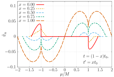
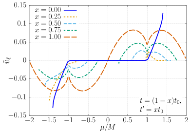
Figure 1: (Color online) The STT coefficients, $v_{n}$ (upper panel) and $v_{\ell}$ (lower panel), as functions of chemical potential $\mu$ for several choices of $x$, where $t=(1-x)\,t_{0}$ and $t^{\prime}=x\,t_{0}$ with $t_{0}/M=0.25$. Plotted are the normalized values, $\tilde{v}_{n}=({\bm{v}}_{n}\cdot{\bm{E}})s_{n}\tilde{\gamma}/(e\hbar|{\bm{E}}|^{2})$ and $\tilde{v}_{\ell}=({\bm{v}}_{\ell}\cdot{\bm{E}})s_{n}\tilde{\gamma}/(e\hbar|{\bm{E}}|^{2})$, where $\tilde{\gamma}=\pi n_{\rm i}u_{\rm i}^{2}/M^{2}$ is the dimensionless damping parameter. The choice $t_{0}/M=0.25$ corresponds to a “strong AF”, in which the upper and lower bands do not overlap. The following features are seen. (i) $v_{n}$ changes sign as $x$ is increased from $x=0$ (AF transport limit) to $x=1$ (FM transport limit), whereas $v_{\ell}$ keeps the same sign throughout. (ii) $v_{\ell}$ coincides with $v_{n}$ at $x=1$. (iii) $v_{n}$ and $v_{\ell}$ are odd functions of $\mu$ at $x=0$ and $1$ because of the presence of particle-hole symmetry, but not for general $x$.

Equation (24) holds for arbitrary values of $t$ and $t^{\prime}$, and incorporate the two opposite transport regimes of AF and FM. In the AF transport limit, $t^{\prime}=0$, one has $\Lambda=(\mu^{2}+M^{2})/(2M^{2})$, and ${\bm{v}}_{n}$ reduces to

$${\bm{v}}_{n}=-\frac{\hbar}{2es_{n}}\,\frac{\mu M}{\mu^{2}-M^{2}}\,\sigma_{xx}{\bm{E}}\qquad(t^{\prime}=0),$$ (26)

where $\sigma_{xx}=2e^{2}D\nu$ is the longitudinal conductivity, $D=\frac{1}{N}\sum_{\bm{k}}(\partial_{x}E_{\bm{k}})^{2}\delta(|\mu|-E_{\bm{k}})\tau/\nu$ is the diffusion constant, $\tau=(1/2)(\gamma_{0}+M\gamma_{3}/\mu)^{-1}$ is the scattering time, and $\nu=\frac{1}{N}\sum_{\bm{k}}\delta(|\mu|-E_{\bm{k}})$ is the density of states per spin, all evaluated at $t^{\prime}=0$. This result agrees with the one reported in Ref. 19.

In the opposite limit, $t=0$, we retrieve the STT for FMs [30, 31]

$${\bm{v}}_{n}=-\frac{\hbar}{2es_{n}}\,(\sigma_{\uparrow}-\sigma_{\downarrow})\,{\bm{E}}\qquad(t=0),$$ (27)

where $\sigma_{\uparrow}$ ($\sigma_{\downarrow}$) is the longitudinal conductivity of electrons in band $\varepsilon^{\prime}_{\bm{k}}-M$ ($\varepsilon^{\prime}_{\bm{k}}+M$). We find that the sign of the STT in the AF transport regime, Eq. (26), is opposite to that in the FM transport regime, Eq. (27).

To see how ${\bm{v}}_{n}$ develops between the AF and the FM regimes, we evaluate Eq. (24) numerically, and plot the result in the upper panel in Fig. 1. We set $t=(1-x)\,t_{0}$ and $t^{\prime}=x\,t_{0}$, which interpolate the AF transport regime ($x\sim 0$) and the FM transport regime ($x\sim 1$). As seen, $v_{n}$ changes sign as $x$ is increased from $x=0$ to 1. This means that the STT due to ${\bm{v}}_{n}$ has opposite sign between FM and AF. This fact has been used in Ref. 19 to interpret the experimental result of domain wall motion in a compensated ferrimagnet GdFeCo, [21] which is expected to be in the AF transport regime [33].

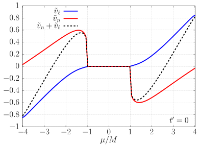
Figure 2: (Color online) Normalized STT coefficients, $\tilde{v}_{n}$ (red), $\tilde{v}_{\ell}$ (blue) and $\tilde{v}_{n}+\tilde{v}_{\ell}$ (black, dashed), calculated with $t/M=1$ and $t^{\prime}=0$. The total Doppler shift $v_{n}+v_{\ell}$ changes sign as a function of $\mu$.

The STT ${\bm{v}}_{\ell}$ arising from the staggered spin density $\langle\hat{\bm{\sigma}}_{n}\rangle$ is calculated by considering the perturbation by the canting moment ${\bm{l}}$ [29]. Unlike the terms with $\beta_{n}$ and $\alpha_{n}$ in Eq. (12) that arise in the presence of spin relaxation, the ${\bm{v}}_{\ell}$-term does not require spin relaxation because it is a reactive STT. In the AF transport limit $t^{\prime}=0$, we obtain

$${\bm{v}}_{\ell} =\frac{\hbar}{2es_{n}}\,M\tau\,\bigg{[}\frac{\mu^{2}-M^{2}}{\mu Dd}+2\zeta\bigg{]}\,\sigma_{xx}{\bm{E}}\ \ \ \ \ (t^{\prime}=0),$$ (28)

to leading order in $\tau$, where $\zeta$ comes from the impurity correction to the ${\bm{l}}$-vertex (see Fig. S1 (c) and Eq. (S12) in SM[32]). Like ${\bm{v}}_{n}$, ${\bm{v}}_{\ell}$ is an odd function of $\mu$ because of opposite spin directions between the upper and lower electron bands, and an odd function of $M$ for a similar reason. As seen in Fig. 1 (blue line in the lower panel) and Fig. 2, the sign of ${\bm{v}}_{\ell}$ relative to ${\bm{E}}$ is negative (hence positive relative to the electron flow) in the lower band, and ${\bm{v}}_{\ell}$ remains finite at the band bottom. These are in contrast to ${\bm{v}}_{n}$. As a result, near the band bottom, the total Doppler shift $({\bm{v}}_{n}+{\bm{v}}_{\ell})/2$ is dominated by ${\bm{v}}_{\ell}$ and hence negative. As the chemical potential is shifted to the AF gap edge, ${\bm{v}}_{n}$ starts to take over and the Doppler shift undergoes a sign change.

In the FM transport limit $t=0$, we find

$${\bm{v}}_{\ell}=-\frac{\hbar}{2es_{n}}(\sigma_{\uparrow}-\sigma_{\downarrow})\,{\bm{E}}\qquad(t=0),$$ (29)

which coincides with ${\bm{v}}_{n}$ in Eq. (27). This fact also indicates that ${\bm{v}}_{\ell}$ needs to be retained as the second STT in AFs. Thus, the AF spin waves receive a Doppler shift by $({\bm{v}}_{n}+{\bm{v}}_{\ell})/2={\bm{v}}_{\ell}$, and this is exactly the Doppler shift in FM.

For other $t$, $t^{\prime}$ values, we have numerically evaluated Eqs. (S27)-(S30) given in SM [32], and the results are plotted in the lower panel in Fig. 1. In contrast to ${\bm{v}}_{n}$, it does not change sign with $x$, hence its sign is always that of FM.

While both ${\bm{v}}_{n}$ and ${\bm{v}}_{\ell}$ appear in the spin-wave Doppler shift, only ${\bm{v}}_{n}$ appears in the collective-coordinate equations of AF domain wall motion. [14, 15, 19] Thus, unlike FM in which there is only one kind of STT, AFs allow for two kinds of STTs that play different roles depending on physical phenomena.

In this Letter, we have studied STTs in AF that induce a Doppler shift in spin-wave spectrum. We have shown that the Doppler shift in AFs is induced by two kinds of reactive STTs, identified as ${\bm{v}}_{n}$ and ${\bm{v}}_{\ell}$, which arise through uniform and staggered electron spin densities, respectively, and are proportional to the spatial gradient of the Néel vector and the uniform moment, respectively. Both STTs contribute to the spin-wave Doppler shift equally. This contrasts with the effects on AF domain walls, to which only ${\bm{v}}_{n}$ is relevant.

We next determined the STTs microscopically using a tight-binding model with n.n. and n.n.n. hopping. In the AF transport regime dominated by n.n. hopping, ${\bm{v}}_{n}$ and ${\bm{v}}_{\ell}$ have opposite signs, and the sign of the Doppler shift depends on band filling. Especially, ${\bm{v}}_{\ell}$ dominates near the band bottom (top), and the sign of the Doppler shift is negative (positive) relative to the applied field ${\bm{E}}$. As the chemical potential is moved toward the AF gap, ${\bm{v}}_{n}$ starts to dominate and the Doppler shift changes sign. In the FM transport limit with only the n.n.n. hopping, both ${\bm{v}}_{n}$ and ${\bm{v}}_{\ell}$ coincide with the well-known STT in FM, and add up to reproduce the Doppler shift in FM.

This work was partly supported by JSPS KAKENHI Grant Numbers JP15H05702, JP17H02929 and JP19K03744, and the Center of Spintronics Research Network of Japan. JJN is supported by a Program for Leading Graduate Schools “Integrative Graduate Education and Research in Green Natural Sciences” and Grant-in-Aid for JSPS Research Fellow Grant Number 19J23587.

References

[1]
A. H. MacDonald and M. Tsoi: Philosophical Transactions of the Royal
Society of London Series A 369 (2011) 3098.
[2]
T. Jungwirth, X. Marti, P. Wadley, and J. Wunderlich: Nature
Nanotechnology 11 (2016) 231.
[3]
O. Gomonay, T. Jungwirth, and J. Sinova: Physica Status Solidi Rapid
Research Letters 11 (2017) 1700022.
[4]
V. Baltz, A. Manchon, M. Tsoi, T. Moriyama, T. Ono, and
Y. Tserkovnyak: Reviews of Modern Physics 90 (2018) 015005.
[5]
M. W. Daniels, R. Cheng, W. Yu, J. Xiao, and D. Xiao: Phys. Rev. B 98 (2018) 134450.
[6]
P. Lederer and D. L. Mills: Phys. Rev. 148 (1966) 542.
[7]
V. Vlaminck and M. Bailleul: Science 322 (2008) 410.
[8]
S.-M. Seo, K.-J. Lee, H. Yang, and T. Ono: Phys. Rev. Lett. 102
(2009) 147202.
[9]
K. Sekiguchi, K. Yamada, S.-M. Seo, K.-J. Lee, D. Chiba, K. Kobayashi, and
T. Ono: Phys. Rev. Lett. 108 (2012) 017203.
[10]
J.-Y. Chauleau, H. G. Bauer, H. S. Körner, J. Stigloher, M. Härtinger,
G. Woltersdorf, and C. H. Back: Phys. Rev. B 89 (2014) 020403.
[11]
A. Roldán-Molina, A. S. Nunez, and R. A. Duine: Phys. Rev. Lett. 118 (2017) 061301.
[12]
A. C. Swaving and R. A. Duine: Phys. Rev. B 83 (2011) 054428.
[13]
Y. Xu, S. Wang, and K. Xia: Phys. Rev. Lett. 100 (2008) 226602.
[14]
K. M. D. Hals, Y. Tserkovnyak, and A. Brataas: Phys. Rev. Lett. 106
(2011) 107206.
[15]
E. G. Tveten, A. Qaiumzadeh, O. A. Tretiakov, and A. Brataas: Phys. Rev. Lett.
110 (2013) 127208.
[16]
Y. Yamane, J. Ieda, and J. Sinova: Phys. Rev. B 94 (2016) 054409.
[17]
H.-J. Park, Y. Jeong, S.-H. Oh, G. Go, J. H. Oh, K.-W. Kim, H.-W. Lee, and
K.-J. Lee: Phys. Rev. B 101 (2020) 144431.
[18]
J. Fujimoto: Phys. Rev. B 103 (2021) 014436.
[19]
J. J. Nakane and H. Kohno: Phys. Rev. B 103 (2021) L180405.
[20]
K.-J. Kim, S. K. Kim, Y. Hirata, S.-H. Oh, T. Tono, D.-H. Kim,
T. Okuno, W. S. Ham, S. Kim, G. Go, Y. Tserkovnyak, A. Tsukamoto,
T. Moriyama, K.-J. Lee, and T. Ono: Nature Materials 16
(2017) 1187.
[21]
T. Okuno, D.-H. Kim, S.-H. Oh, S. K. Kim, Y. Hirata, T. Nishimura, W. S. Ham,
Y. Futakawa, H. Yoshikawa, A. Tsukamoto, Y. Tserkovnyak, Y. Shiota,
T. Moriyama, K.-J. Kim, K.-J. Lee, and T. Ono: Nature Electronics 2 (2019) 389.
[22]
D.-H. Kim, S.-H. Oh, D.-K. Lee, S. K. Kim, and K.-J. Lee: Phys. Rev. B
103 (2021) 014433.
[23]
E. M. Lifshitz and L. P. Pitaevskii: Statistical Physics, Part II, Course
of Theoretical Physics (Pergamon, Oxford, 1980).
[24]
E. G. Tveten, T. Müller, J. Linder, and A. Brataas: Phys. Rev. B 93 (2016) 104408.
[25]
F. D. M. Haldane: Phys. Rev. Lett. 50 (1983) 1153.
[26]
It seems customary to define and by making the sum and
the difference of two spins in a unit cell.[34] The uniform
magnetization thus defined contains an unphysical component (called
“intrinsic magnetization” in Ref. 24), which has been
subtracted to define the physical magnetization in
Ref. 35. The uniform moment defined by Eq. (4)
coincides with the physical magnetization introduced in
Ref. 35 for slowly-varying textures. In this Letter, we drop
the tilde in and simply write .
[27]
In fact, the -term is often overlooked in the literature. Few
exceptions are Ref. 14, where the authors dropped it by
discussing its reciprocal counterpart is small, and Ref.
18, which retained it but without discussing approximation
criterion .
[28]
G. Tatara, H. Kohno, and J. Shibata: Physics Reports 468 (2008)
213.
[29]
J. J. Nakane, K. Nakazawa, and H. Kohno: Phys. Rev. B 101 (2020)
174432.
[30]
H. Kohno, G. Tatara, and J. Shibata: Journal of the Physical Society of Japan
75 (2006) 113706.
[31]
H. Kohno and J. Shibata: Journal of the Physical Society of Japan 76 (2007) 063710.
[32]
(Supplementary material) Calculations of and are
provided online.
[33]
J. Park, Y. Hirata, J.-H. Kang, S. Lee, S. Kim, C. Van Phuoc, J.-R. Jeong,
J. Park, S.-Y. Park, Y. Jo, A. Tsukamoto, T. Ono, S. K. Kim, and K.-J. Kim:
Phys. Rev. B 103 (2021) 014421.
[34]
H. J. Mikeska and M. Steiner: Advances in Physics 40 (1991)
191.
[35]
J. J. Nakane and H. Kohno: Journal of the Physical Society of Japan 90 (2021) 034702.