Phase transitions in one-dimensional correlated Fermi gases with cavity-induced umklapp scattering

Abstract

The phase transitions of one dimensional correlated Fermi gases in a transversely driven optical cavity, under the umklapp condition that the cavity wavenumber equals two times of Fermi wavenumber, are studied with the bosonization and renormalization group (RG) techniques. The bosonization of Fermi fields gives rise to an all-to-all sine-Gordon (SG) model due to the cavity-assisted non-local interactions, where the Bose fields at any two spatial points are coupled. The superradiant phase transition is then linked to the Kosterlitz–Thouless (KT) phase transition of the all-to-all SG model. The nesting effect, in which the superradiant phase transition can be triggered by infinitely small atom-cavity coupling strength, is preserved for any non-attractive local interactions. The phase transition occurs at finite critical coupling strength for attractive local interactions. Nevertheless, the critical dimension of the KT phase transition is also $2$ like that in an ordinary local SG model. Our work provides an analytical framework for understanding the phase transitions in correlated intra-cavity Fermi gases.

I Introduction

The quantum gases in an optical cavity provide new paradigms for exploring many-body physics Ritsch et al. (2013); Mivehvar et al. (2021). The self-organization of atoms into a checkerboard order, accompanying the superradiant macroscopic occupation of cavity modes, occurs above a critical atom-cavity coupling strength Baumann et al. (2010); Klinder et al. (2015). For Bose-Einstein condensate (BEC), the superradiant phase transition is approximately characterized by a generalized Dicke model since atoms only condensate into the several resonant modes Baumann et al. (2010). The superradiant phase transition of Fermi gases (and hard-core bosons Rylands et al. (2020)) shows distinct features due to the presence of Fermi surface Piazza and Strack (2014); Keeling et al. (2014); Chen et al. (2014); Pan et al. (2015); Mivehvar et al. (2017); Yu et al. (2018); Zhang et al. (2021). For example, when the Fermi surface is commensurate with the cavity wave length $k_{0}=2k_{F}$ ($k_{F}$ is the Fermi wave number), i.e., the atoms are scattered by cavity photons with the umklapp condition, the nesting effect that the critical point softens to zero is predicted Piazza and Strack (2014); Keeling et al. (2014); Chen et al. (2014). Recently, the superradiant phase transition of Fermi gases was observed experimentally Zhang et al. (2021).

The cavity-induced spontaneous symmetry breaking in intra-cavity quantum gases in general can be interpreted with the effective atom-atom interaction generated by the adiabatical elimination of cavity dynamics Habibian et al. (2013); Gopalakrishnan et al. (2009); Léonard et al. (2017); Mivehvar et al. (2019), upon the picture of cavity-induced dynamical potentials Mivehvar and Feder (2014); Padhi and Ghosh (2014); Dong et al. (2014); Deng et al. (2014); Pan et al. (2015); Kroeze et al. (2019); Zheng and Cooper (2016); Kollath et al. (2016); Sheikhan et al. (2016); Gulácsi and Dóra (2015); Zheng and Cooper (2016); Ballantine et al. (2017). Although the fluctuations of single-mode cavity field in the suprradiant phases in the thermal dynamic limit is ignorable, due to the cavity modes essentially have no spatial dynamics Piazza et al. (2013), the interplay of cavity-assisted non-local and local interactions in low-dimension correlated quantum gases is still under exploring Landig et al. (2016). The supperadiant phase transition of Fermi gases crossing Feshbach resonance shows smooth crossover between the BCS and BEC regimes Chen et al. (2015); Yu et al. (2018). Experimentally preparing strong correlated Fermi gases in an optical cavity calls for further study on the interplay between correlation effects and cavity-induced dynamics Roux et al. (2020, 2021).

In this paper, we theoretically study the phase transitions of one-dimensional (1D) correlated Fermi gases trapped in an optical cavity with the bosonization and renormalization group techniques. We focus on the nesting point where the Fermi surface has a wave length commensurate with the cavity wave length, i.e., $k_{0}=2k_{F}$. The bosonization of the Fermi fields gives rise to an all-to-all sine-Gordon model, in which the Bose fields in any distances are coupled. The superradiant phase transition is then linked to the well-known $(1+1)$-dimensional KT phase transition of SG model. By employing the perturbative renormalization group techniques, we capture the ground-state phase diagram of the Fermi gas. The nesting effect, where the model shows vanishing critical coupling strength, survives only with repulsive local interaction. The critical coupling strength become finite when the local interaction becomes attractive. Nevertheless, we find the critical dimension of the KT phase transition is also $2$, the same with that in an ordinary local SG model.

In the following, we present the model and its bosonization in section II and III, respectively. Further, we perform the RG analysis in section IV, discuss the phase diagram in section V, and analyze the critical dimension in section VI. A brief summary is given in the last section.

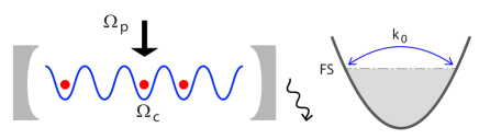
Figure 1: Illustration of the model. The 1D Fermi gas is coupled with the cavity field ($\Omega_{c}$) via a transverse driving ($\Omega_{p}$). The atoms are assumed to have two energy levels (not shown), and the higher level has been adiabatically eliminated since the driving and cavity fields are far detuning from the energy levels. The Fermi surface (FS) is assumed to be resonant with the cavity field, i.e., $k_{0}=2k_{f}$.

II Model

We consider an 1D Fermi gas of two-level fermions loaded in a single-mode optical cavity [see Fig. 1], where the atomic and cavity dynamics are coupled through the scattering of a transverse driving field $\Omega_{p}$ by atoms into the cavity. The single-photon detuning $\Delta$ (i.e., the frequency differences between the energy-level difference and the light fields) is assumed to be far larger than other energy scales and then the higher level can be adiabatically eliminated. The model Hamiltonian thus is given by

$$\begin{split}\hat{H}=&\int dx\hat{\psi}^{\dagger}(x)[-\frac{\nabla^{2}}{2m}-\mu+V_{0}\hat{a}^{\dagger}\hat{a}\cos^{2}(k_{0}x)]\hat{\psi}(x)\\ &+\eta\left(\hat{a}^{\dagger}+\hat{a}\right)\int dx\hat{n}(x)\cos\left(k_{0}x\right)-\Delta_{c}\hat{a}^{\dagger}\hat{a}\\ &+\int\int dxdrU(|r|):\hat{n}(x)\hat{n}(x-r):,\end{split}$$ (1)

where $\hat{\psi}$ and $\hat{a}$ are the field operators for atoms and cavity photons, $\mu$ is the chemical potential of fermions, $V_{0}=\Omega_{c}^{2}/\Delta$ term with density operator $\hat{n}=\hat{\psi}^{\dagger}\hat{\psi}$ and single-photon Rabi frequency $\Omega_{c}$ represents the stark shift induced by the cavity field, $\eta=\Omega_{c}\Omega_{p}/\Delta$ with the Rabi frequency of pumping field $\Omega_{p}$ is the atom-cavity coupling strength, $\Delta_{c}$ is the two-photon detuning (i.e., the frequency difference between the cavity mode and pumping field), and the last term is the local interaction. Here the symbol $:\cdots:$ denotes the normal order.

The dynamics of cavity mode $\hat{a}$ can be captured by the Heisenberg-Langevin equation,

$$i\hbar\dot{\hat{a}}=-(\tilde{\Delta}_{c}+i\kappa)\hat{a}+\eta\int dx\hat{n}(x)\cos\left(k_{0}x\right)+\sqrt{2\kappa}\hat{a}_{in}(t),$$ (2)

where $\tilde{\Delta}_{c}=\Delta_{c}+V_{0}\int dx\hat{\psi}^{\dagger}(x)\cos^{2}\left(k_{0}x\right)\hat{\psi}(x)$, $\kappa$ describes the decay of the cavity and $\hat{a}_{in}(t)$ satisfying $\langle\hat{a}_{in}\rangle=0$ and $\langle\hat{a}_{in}(t)\hat{a}_{in}^{\dagger}(t^{{}^{\prime}})\rangle=\delta(t-t^{{}^{\prime}})$ is the Langevin operator Carmichael (2009); Habibian et al. (2011, 2013); Sieberer et al. (2016). We assume the optical cavity has a far shorter characterisitc time $\delta t_{c}$ due to the large $\kappa$ and $\Delta_{c}$ with respect to the energy scales in atomic dynamics. Then the adiabatic elimination of the cavity mode is applicable and it leads to the relation,

$$\hat{a}\approx\frac{\eta\int dx\hat{n}(x)\cos\left(k_{0}x\right)}{\tilde{\Delta}_{c}+i\kappa},$$ (3)

by taking the coarse graining $\delta t_{c}^{-1}\int_{t-\delta t_{c}/2}^{t+\delta t_{c}/2}dt^{{}^{\prime}}\hat{A}(t^{{}^{\prime}})\approx\hat{A}(t^{{}^{\prime}})$ and assuming $\delta t_{c}^{-1}\int_{t-\delta t_{c}/2}^{t+\delta t_{c}/2}dt^{{}^{\prime}}\dot{\hat{a}}(t^{{}^{\prime}})$ is ignorable in the dynamical equation Rojan et al. (2016). By substituting Eq. (3) into Eq. (4), we derive

$$\begin{split}\hat{H}\approx&\int dx\hat{\psi}^{\dagger}(x)[-\frac{\hbar^{2}\nabla^{2}}{2m}-\mu+V_{0}\hat{n}(x)]\hat{\psi}(x)\\ &+\eta_{eff}\int dxdx^{{}^{\prime}}:\hat{n}(x)\hat{n}(x^{{}^{\prime}}):\cos(k_{0}x)\cos(k_{0}x^{{}^{\prime}})\\ &+\int\int dxdrU(|r|):\hat{n}(x)\hat{n}(x-r):,\end{split}$$ (4)

where $\eta_{eff}\approx 2\eta^{2}\Delta_{c}/(\Delta_{c}^{2}+\kappa^{2})$, after neglecting the Stark shift term by assuming $|\Delta_{c}|\gg V_{0}$ for simplicity. The second term is the cavity-assisted non-local interaction. We would like to note that, in finite-temperature systems, the integration of cavity fields will leave a time-dependent cavity-assisted interaction term Piazza et al. (2013).

III Bosonization

The single-particle spectra of the Fermi gas have a quadratic dispersion with a Fermi surface determined by the chemical potential $\mu$ at zero temperature [see Fig. 1]. The low-energy dynamics mainly involves the single-particle modes at around the Fermi surface, and then the single-particle part [i.e., the first term in Eq. (4)] can be approximately simulated by a linearized Hamiltonian,

$$\hat{H}_{1}=\sum_{k,s=\pm 1}s\upsilon_{f}:\hat{c}_{sk}^{\dagger}\hat{c}_{sk}:=\upsilon_{f}\sum_{s}\int dx:\hat{\psi}_{s}^{\dagger}(-is\partial_{x})\hat{\psi}_{s}:,$$ (5)

where $\hat{c}_{sk}=L^{-1/2}\int dx\hat{\psi}_{s}e^{is(k+k_{f})x}$ with $s=\pm$ and system length $L$ (also the range of spatial integrals) and $\upsilon_{f}$ is the first-order dispersion coefficient at around the Fermi surface. $\hat{H}_{0}$ can be further bosonized as

$$\hat{H}_{1}\approx\frac{\upsilon_{f}}{2}\sum_{s}[\int dx:(\partial_{x}\hat{\phi}_{s})^{2}:+\frac{2\pi}{L}\Delta\hat{N}_{s}(\Delta\hat{N}_{s}+1)],$$ (6)

with the bosonization relation,

$$\hat{\psi}_{\pm}=\frac{\hat{F}_{\pm}}{\sqrt{2\pi\alpha}}e^{\pm 2\pi i\Delta\hat{N}_{\pm}x/L}e^{-i\sqrt{2\pi}\hat{\phi}_{\pm}(x)},$$ (7)

where $\hat{\phi}_{s}$, $\hat{F}_{s}$, $\Delta\hat{N}_{s}$ and $\alpha$ are the Bose field operators, Klein factors, number operators and factor to violate the ultraviolet divergence (the minimum spatial resolution, which in general is set as the lattice constant in lattice model), respectively Von Delft and Schoeller (1998); Gogolin et al. (2004).

The atom-cavity term [i.e., the second term in Eq. (4)] is expanded into,

$$\begin{split}&\hat{H}_{2}=\frac{\eta_{eff}}{2}\sum_{s_{1}\cdots s_{4}=\pm 1}\int dxdr[\cos(2k_{0}x)+\cos(k_{0}r)]\\ &\times:\hat{\psi}_{s_{1}}^{\dagger}(x+\frac{r}{2})\hat{\psi}_{s_{3}}^{\dagger}(x-\frac{r}{2})\hat{\psi}_{s_{4}}(x-\frac{r}{2})\hat{\psi}_{s_{2}}(x+\frac{r}{2}):\\ &\times e^{ik_{f}(s_{2}+s_{4}-s_{1}-s_{3})x+ik_{f}(s_{2}+s_{3}-s_{1}-s_{4})r/2},\end{split}$$ (8)

with $\hat{\psi}=\sum_{s}e^{isk_{f}x}\hat{\psi}_{s}$. In order to make the expressions in the summation non-vanishing, $s_{2}+s_{4}-s_{1}-s_{3}$ and $s_{2}+s_{3}-s_{1}-s_{4}$ have to be $\pm 4$ and $0$, or $0$ and $\pm 4$, which are only satisfied by $(s_{1},s_{2},s_{3},s_{4})=(1,-1,1,-1)$, or $(1,-1,-1,1)$, or $(-1,1,1,-1)$, or $(-1,1,-1,1)$. By employing Eq. (7), we finally derive the bosonized Hamiltonian,

$$\hat{H}_{2}=\frac{\xi}{L}\int\int dxdr\cos(2\sqrt{\pi}\phi^{(+)})\cos(2\sqrt{\pi}\phi^{(-)}),$$ (9)

where $\phi=(\phi_{1}-\phi_{-1})/\sqrt{2}$, $\theta=(\phi_{1}+\phi_{-1})/\sqrt{2}$, the simplified expression $f^{(\pm)}=f(x\pm r/2,\tau)$ is used, $\xi=L\eta_{eff}/(4\pi\alpha)^{2}$ by considering $\Omega_{c}$ is proportional to the cavity length and further is proportional to the system size in the thermal dynamics . It is necessary to scale the strength of cavity-atom coupling $\xi$ with the system length $L$ to avoid the energy divergence.

The local interaction term [i.e., the last term in Eq. (4)] is transformed into

$$\begin{split}\hat{H}_{3}=&\sum_{s_{1}\cdots s_{4}=\pm 1}\int\int dxdrU(r)e^{ik_{f}[(s_{2}+s_{4}-s_{1}-s_{3})x+(s_{3}-s_{4})r]}\\ &\times:\hat{\psi}_{s_{1}}^{\dagger}(x)\hat{\psi}_{s_{3}}^{\dagger}(x-r)\hat{\psi}_{s_{4}}(x-r)\hat{\psi}_{s_{2}}(x):.\end{split}$$ (10)

Assuming the characteristic length of $U(|r|)$ is far larger than $2\pi/k_{f}$ but is far smaller than system size, then we can approximately derive

$$\hat{H}_{3}\approx U_{0}\int dx:(\partial_{x}\phi)^{2}:,$$ (11)

where $U_{0}$ is the interaction coefficient.

We finally derive the bosonized Hamiltonian,

$$\begin{split}\hat{H}=&\sum_{n=1}^{3}\hat{H}_{n}=\frac{u}{2}\int dx[g(\partial_{x}\theta)^{2}+g^{-1}(\partial_{x}\phi)^{2}]\\ &+\frac{\xi}{L}\int\int dxdr\cos(2\sqrt{\pi}\phi^{(+)})\cos(2\sqrt{\pi}\phi^{(-)}),\end{split}$$ (12)

where the effective velocity $u=\sqrt{\upsilon_{f}(\upsilon_{f}+2U_{0})}$ and the Luttinger parameter $g=\sqrt{\upsilon_{f}/(\upsilon_{f}+2U_{0})}$. $g>1$ ($g<1$) correspond to the attractive (repulsive) local interactions, respectively.

The Lagrange of our model takes the form,

$$\begin{split}\mathcal{L}=&-i\partial_{x}\theta\partial_{\tau}\phi+\frac{u}{2}[g(\partial_{x}\theta)^{2}+g^{-1}(\partial_{x}\phi)^{2}]\\ &+\frac{\xi}{L}\int\int dr\cos(2\sqrt{\pi}\phi^{(+)})\cos(2\sqrt{\pi}\phi^{(-)}),\end{split}$$ (13)

with the imaginary time $\tau$ under the convention of action $S=\int\int dxd\tau\mathcal{L}$ and partition function $Z=\int\mathcal{D}[\phi,\theta]e^{-S}$. By integrating the field $\theta$, we yield

$$\begin{split}\mathcal{L}=&\frac{1}{2g}[u^{-1}(\partial_{\tau}\phi)^{2}+u(\partial_{x}\phi)^{2}]\\ &+\frac{\xi}{L}\int dr\cos(2\sqrt{\pi}\phi^{(+)})\cos(2\sqrt{\pi}\phi^{(-)}).\end{split}$$ (14)

This is an all-to-all sine-Gordon model in the sense that two fields with any distances are coupled in the sine term.

IV Renormalization group analysis

An (1+1)-dimensional SG model in general has a phase transition at a critical coupling strength, which belongs to the same universality class of KT phase transition in two-dimensional XY model and superfluids, and also characterizes the metal-insulator transition of topological edge states in topological matters Gogolin et al. (2004); Wen (2004); Cheng (2012), etc.. The superradiant phase transition is linked to the (1+1)-dimensional KT phase transition of the all-to-all SG model, where the normal or superradiant phases correspond to the irrelevant (gapless) and relevant (gapped) regimes of the sine term. Inspired by this interesting connection, we will analyze the KT phase transition of the all-to-all SG model in Eq. (14) with perturbative renormalization group technique below.

For discussion convenience, we define $\boldsymbol{x}=(x,-\tau)$ and $\boldsymbol{k}=(k,\omega)$, where $k$ and $\omega$ are the momentum and frequency. To figure out the renormalization process, we set a cutoff $\sqrt{u^{-1}\omega^{2}+uk^{2}}<\Lambda$ on the momentum-frequency plane and denote the field with $\phi_{\Lambda}(\boldsymbol{x})$. The strategy for the perturbative renormalization is standard: 1) expanding the field into low-frequency and high-frequency parts, and integrating out the high-frequency part; 2) rescaling the dimensions back to the same cutoff and then obtaining the renormalization equations.

The field can be expanded into the high and low-frequency components,

$$\phi_{\Lambda}=\frac{1}{\sqrt{\beta L}}(\sum_{|\boldsymbol{k}|<\Lambda^{{}^{\prime}}}+\sum_{\Lambda^{{}^{\prime}}<|\boldsymbol{k}|<\Lambda})\phi_{\boldsymbol{k}}e^{i\boldsymbol{k}\cdot\boldsymbol{x}}=\phi_{\Lambda^{{}^{\prime}}}(\boldsymbol{x})+h(\boldsymbol{x}),$$ (15)

with $\delta\Lambda=\Lambda-\Lambda^{{}^{\prime}}\ll\Lambda$.

First, we need to calculate the effective action for $\phi_{\Lambda^{{}^{\prime}}}$ by integrating out $h$ field. As the action $S[h]$ is in the quadratic form, it directly gives $\langle\phi_{\boldsymbol{k}}\phi_{\boldsymbol{k}^{{}^{\prime}}}\rangle_{h}=(u^{-1}\omega^{2}+up^{2})^{-1}\delta_{\boldsymbol{k}^{{}^{\prime}},-\boldsymbol{k}}$, and

$$\begin{split}\langle h^{(\lambda)}h^{(\lambda^{{}^{\prime}})}\rangle_{h}&=\frac{g}{\beta L}\sum_{\Lambda^{{}^{\prime}}<|\boldsymbol{k}|,|\boldsymbol{k}^{{}^{\prime}}|<\Lambda}\frac{\delta_{\boldsymbol{k}^{{}^{\prime}},-\boldsymbol{k}}e^{i(\boldsymbol{k}\cdot\boldsymbol{x}^{(\lambda)}+\boldsymbol{k}^{{}^{\prime}}\cdot\boldsymbol{x}^{(\lambda^{{}^{\prime}})})}}{u^{-1}\omega^{2}+up^{2}}\\ &=G_{\lambda\lambda^{{}^{\prime}}}dl+\mathcal{O}(dl^{2}),\quad\lambda,\lambda^{{}^{\prime}}=\pm,\end{split}$$ (16)

where $dl=\ln(\Lambda/\Lambda^{{}^{\prime}})$, $G_{++}=G_{--}=g/(2\pi)$ and $G_{+-}=G_{+-}\approx gJ_{0}(\Lambda r/\sqrt{u})/(2\pi)$. Then it leads to

$$\begin{split}&\langle\delta S\rangle_{h}=\frac{\xi(1-2gdl)}{L}\int d^{2}\boldsymbol{x}dr\cos(2\sqrt{\pi}\phi_{\Lambda^{{}^{\prime}}}^{(+)})\cos(2\sqrt{\pi}\phi_{\Lambda^{{}^{\prime}}}^{(-)})\\ &+\frac{2g\xi dl}{L}\int d^{2}\boldsymbol{x}drJ_{0}(\frac{\Lambda r}{\sqrt{u}})\sin(2\sqrt{\pi}\phi_{\Lambda^{{}^{\prime}}}^{(+)})\sin(2\sqrt{\pi}\phi_{\Lambda^{{}^{\prime}}}^{(-)}).\end{split}$$ (17)

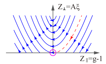
Figure 2: Phase diagram. The red dashed curve is the marginal direction for the relevant regime. The red circle indicates the nesting effect (infinitely small critical coupling strength) in free Fermi gases predicted with the Landau theory of phase transition Piazza and Strack (2014); Keeling et al. (2014); Chen et al. (2014). The phase diagram shows that the nesting effect survives for non-attractive local interactions ($g<1$) only.

Noting that $J_{0}(\Lambda r/\sqrt{u})$ quickly decay with $r$ from $r=0$ as $\Lambda$ is large, we have $2\sin(2\sqrt{\pi}\phi_{\Lambda^{{}^{\prime}}}^{(+)})\sin(2\sqrt{\pi}\phi_{\Lambda^{{}^{\prime}}}^{(-)})\approx 1-2\pi r^{2}(\partial_{x}\phi_{\Lambda^{{}^{\prime}}})^{2}-\cos(4\sqrt{\pi}\phi_{\Lambda^{{}^{\prime}}})$. Ignoring the irrelevant terms and rescaling the dimensions as $\boldsymbol{k}\rightarrow\Lambda\boldsymbol{k}/\Lambda^{{}^{\prime}}$ and $\boldsymbol{x}\rightarrow\Lambda^{{}^{\prime}}\boldsymbol{x}/\Lambda$ (note that the system size $L$ is also rescaled), and on the other hand, considering the scaling of $u$ can be absorbed by redefining the coordinates, we yield the following effective lagrangian

$$\begin{split}\mathcal{L}_{eff}=&\frac{1}{2g^{{}^{\prime}}}[u^{-1}(\partial_{\tau}\phi_{\Lambda})^{2}+u(\partial_{x}\phi_{\Lambda})^{2}]\\ &+\frac{\xi^{{}^{\prime}}}{L}\int dr\cos(2\sqrt{\pi}\phi_{\Lambda}^{(+)})\cos(2\sqrt{\pi}\phi_{\Lambda}^{(-)}),\end{split}$$ (18)

where $g^{{}^{\prime}-1}=[1-2Ag^{2}\xi dl/L]^{1/2}g^{-1}$, and $\xi^{{}^{\prime}}=\xi[1+2(1-g)dl]$, and non-universal coefficient $A=2\pi\int drr^{2}J_{0}(\Lambda r/\sqrt{u})$. Then the renormalization equations (i.e., the KT equations) are given by

$$\frac{d\xi}{dl}=2(1-g)\xi,\quad\frac{dg}{dl}=A\xi g^{3},$$ (19)

Unlike an ordinary SG model Gogolin et al. (2004), where the complete RG equations for both the coupling strength and interactions can only obtained with both the one-order and second-order perturbations, the all-to-all SG model is not renormalizable for second-order perturbations.

V Phase diagram

Obviously, the critical point is $g=1$ when $\xi\rightarrow 0$. When $g\geq 1$, the perturbation of sine term is relevant. It implies the phase transition even occurs with infinitely small coupling strength $\xi$, even at the free limit $g=1$, which is consistent with the nesting effect in the superradiant phase transition of degenerate Fermi gases Piazza and Strack (2014); Keeling et al. (2014); Chen et al. (2014), but is inherently different to the ordinary local SG model with critical point at $g>1$.

The invariant points are given by $\xi=0$. At around the unstable invariant point $g=1$ and $\xi=0$, we define the small fluctuations of parameters

$$z_{\parallel}=g-1,\quad z_{\perp}=A\xi.$$ (20)

The linearized RG equations can be derived in the following forms,

$$\frac{dz_{\perp}}{dl}=-2z_{\parallel}z_{\perp},\quad\frac{dz_{\parallel}}{dl}=-z_{\perp},$$ (21)

which allows us to plot the phase diagram on the plane of $z_{\parallel}$-$z_{\perp}$ like the ordinary SG model, as shown in Fig. 2. The quantity $C=z_{\perp}-z_{\parallel}^{2}$ is invariant along the renormalization flow. The phase boundary is a quadratic curve [see the red dashed curve in Fig. 2].

VI Critical dimension

Now let us go forward to the analysis of scaling dimension of the all-to-all sine term follow the Ref. Gogolin et al. (2004). By redefining the fields $\phi/\sqrt{g}\rightarrow\phi$, the Luttinger parameter $g$ will be absorbed into the sine term:

$$\begin{split}\mathcal{L}=&\frac{1}{2}[u^{-1}(\partial_{\tau}\phi)^{2}+u(\partial_{x}\phi)^{2}]\\ &+\frac{\xi}{L}\int dr\cos(\Gamma\phi^{(+)})\cos(\Gamma\phi^{(-)}),\end{split}$$ (22)

with $\Gamma=2\sqrt{\pi g}$. For the free field $S_{0}=\int\int dxd\tau[u^{-1}(\partial_{\tau}\phi)^{2}+u(\partial_{x}\phi)^{2}]/2$, the generating functional of fields $\phi$ is given by

$$\begin{split}Z[h]=&\int\mathcal{D}[\phi(\boldsymbol{x})]e^{-S_{0}-\int dxd\tau h{\boldsymbol{x}}\phi(\boldsymbol{x})}\\ &=Z[0]\exp[\frac{1}{2}\int\int d\boldsymbol{x}d\boldsymbol{x}^{{}^{\prime}}h(\boldsymbol{x})G_{0}(\boldsymbol{x},\boldsymbol{x}^{{}^{\prime}})h(\boldsymbol{x}^{{}^{\prime}})],\end{split}$$ (23)

where $G(\boldsymbol{x},\boldsymbol{x}^{{}^{\prime}})$ is the Green’s function satisfying $-(u^{-1}\partial_{\tau}^{2}+u\partial_{x}^{2})G_{0}(\boldsymbol{x},\boldsymbol{x}^{{}^{\prime}})=\delta(\boldsymbol{x}-\boldsymbol{x}^{{}^{\prime}})$. With the complex coordinates $z=\tau+ix/u$ and $\bar{z}=\tau-ix/u$, the Green’s function takes the form,

$$G_{0}(z,\bar{z})=\frac{1}{4\pi}\ln(\frac{R^{2}}{z\bar{z}+\alpha^{2}}).$$ (24)

Note that $G(\boldsymbol{x},\boldsymbol{x}^{{}^{\prime}})$ only depends on the difference $(\boldsymbol{x}-\boldsymbol{x}^{{}^{\prime}})$ denoted by $z$ and $\bar{z}$ in the above equation.

For a particular choice, $h=h_{0}=i\sum_{j=1}^{N}\Gamma_{j}\delta(\boldsymbol{x}-\boldsymbol{x}_{j})$, the generating functional is given by

$$\begin{split}&\mathcal{F}(1,2,\dots,N)=Z[h_{0}]/Z[0]\\ &=\Pi_{i>j}(\frac{z_{ij}\bar{z}_{ij}}{\alpha^{2}})^{\Gamma_{i}\Gamma_{j}/4\pi}(\frac{R}{\alpha})^{-(\sum_{j}\Gamma_{j})^{2}/4\pi},\end{split}$$ (25)

where $z_{ij}=z_{i}-z_{j}$. To make $\mathcal{F}$ non-vanishing, it requires $\sum_{j}\Gamma_{j}=0$, since $R/\alpha\rightarrow\infty$ in the thermodynamics limit. These basic results all can be found in the Ref. Gogolin et al. (2004).

We are mainly interesting the all-to-all sine term $\hat{B}(\boldsymbol{x})=\frac{\xi}{L}\int dr\cos(\Gamma\hat{\phi}^{(+)})\cos(\Gamma\hat{\phi}^{(-)})$ here. According to the above results, the correlation function of $\hat{B}(\boldsymbol{x})$ can be written as

$$\begin{split}&\langle\hat{B}(\boldsymbol{x})\hat{B}^{\dagger}(\boldsymbol{x}^{{}^{\prime}})\rangle=\frac{\xi^{2}}{16L^{2}}\sum_{\sigma_{1},\cdots,\sigma_{4}=\pm 1}\int\int drdr^{{}^{\prime}}\\ &\quad\quad\quad\quad\quad\quad\quad\times\langle e^{i\Gamma\sigma_{1}\hat{\phi}^{(+)}}e^{i\Gamma\sigma_{2}\hat{\phi}^{(-)}}e^{i\Gamma\sigma_{3}\hat{\phi}^{(+),}}e^{i\Gamma\sigma_{4}\hat{\phi}^{(-),}}\rangle\\ &=\frac{\xi^{2}}{16L^{2}}\sum_{\sigma_{1}+\sigma_{2}+\sigma_{3}+\sigma_{4}=0}\int\int drdr^{{}^{\prime}}\Pi_{i>j}(\frac{z_{ij}\bar{z}_{ij}}{\alpha^{2}})^{\Gamma_{i}\Gamma_{j}/4\pi},\end{split}$$ (26)

where we have defined $\hat{\phi}(z_{1,2},\bar{z}_{1,2})=\hat{\phi}^{(\pm)}$, $\hat{\phi}(z_{3,4},\bar{z}_{3,4})=\hat{\phi}^{(\pm)^{\prime}}=\hat{\phi}(x^{{}^{\prime}}\pm\frac{r^{{}^{\prime}}}{2},\tau)$, $\Gamma_{j}=\sigma_{j}\Gamma$ and $z_{ij}=z_{i}-z_{j}$.

The condition $\sigma_{1}+\sigma_{2}+\sigma_{3}+\sigma_{4}=0$ requires $\sigma_{j}$s appear in pairs with opposite signs. Then for any sets of $\sigma_{j}$, the six terms in the continued product in Eq. (26) have four terms with powers of $-\Gamma^{2}/4\pi$ and two terms with powers of $\Gamma^{2}/4\pi$. For the scaling transformation $\boldsymbol{x}\rightarrow\lambda\boldsymbol{x}$ and $L\rightarrow\lambda L$, the correlation function $\langle\hat{B}(\boldsymbol{x})\hat{B}^{\dagger}(\boldsymbol{x}^{{}^{\prime}})\rangle$ is scaled as $\lambda^{\Gamma^{2}/\pi}\langle\hat{B}(\boldsymbol{x})\hat{B}^{\dagger}(\boldsymbol{x}^{{}^{\prime}})\rangle$. Therefore, the scaling dimension of the all-to-all sine term $\hat{B}(\boldsymbol{x})$ is $d=\Gamma^{2}/2\pi=2g$ Gogolin et al. (2004); Francesco et al. (2012). The above GR analysis then further leads to the conclusion that the critical dimension for the KT phase transition is $d_{c}=2g_{c}=2$, which is the same with an ordinary local SG model Gogolin et al. (2004), although the all-to-all SG model involves infinitely long-range coupling. It implies that only the phase transitions in all-to-all models with dimensions larger than $2$ can be well characterized with mean-field theory.

VII Conclusion

We theoretically analyze the phase transitions of 1D correlated Fermi gases with cavity-induced umklapp scattering, based on the bosonization and renormalization group techniques. An all-to-all SG model is derived with the bosonization of Fermi fields. The superradiant phase transition is linked to the (1+1)-dimensional KT phase transition of the SG model. The phase diagram given by RG analysis shows that the nesting effect is preserved only with non-attractive interactions. For attractive Fermi gas, the critical coupling strength becomes finite. The critical dimension for the KT phase transition of the all-to-all SG model is also $2$, like that in an ordinary local sine-Gordon model. Our results are consistent with the studies on infinite-range coupling Heisenberg chains Li et al. (2021) and Ising models Binney et al. (1992), as well as the Fermi gases with BCS-BEC crossover Chen et al. (2015); Yu et al. (2018), and are easily extended to the case of hard-core bosons Rylands et al. (2020).

Acknowledgements.–The author thanks Yu Chen, Jiangbin Gong, Qingze Guan and Jianwen Jie for the helpful discussions. This work is supported by the National Natural Science Foundation of China (Grant No. 11904228) and the Science Specialty Program of Sichuan University (Grand No. 2020SCUNL210).

References

- Ritsch et al. (2013) H. Ritsch, P. Domokos, F. Brennecke, and T. Esslinger, Reviews of Modern Physics 85, 553 (2013).
- Mivehvar et al. (2021) F. Mivehvar, F. Piazza, T. Donner, and H. Ritsch, arXiv preprint arXiv:2102.04473 (2021).
- Baumann et al. (2010) K. Baumann, C. Guerlin, F. Brennecke, and T. Esslinger, Nature 464, 1301 (2010).
- Klinder et al. (2015) J. Klinder, H. Keßler, M. R. Bakhtiari, M. Thorwart, and A. Hemmerich, Physical Review Letters 115, 230403 (2015).
- Rylands et al. (2020) C. Rylands, Y. Guo, B. L. Lev, J. Keeling, and V. Galitski, Physical Review Letters 125, 010404 (2020).
- Piazza and Strack (2014) F. Piazza and P. Strack, Physical Review Letters 112, 143003 (2014).
- Keeling et al. (2014) J. Keeling, M. Bhaseen, and B. Simons, Physical Review Letters 112, 143002 (2014).
- Chen et al. (2014) Y. Chen, Z. Yu, and H. Zhai, Physical Review Letters 112, 143004 (2014).
- Pan et al. (2015) J.-S. Pan, X.-J. Liu, W. Zhang, W. Yi, and G.-C. Guo, Physical Review Letters 115, 045303 (2015).
- Mivehvar et al. (2017) F. Mivehvar, H. Ritsch, and F. Piazza, Physical Review Letters 118, 073602 (2017).
- Yu et al. (2018) D. Yu, J.-S. Pan, X.-J. Liu, W. Zhang, and W. Yi, Frontiers of Physics 13, 1 (2018).
- Zhang et al. (2021) X. Zhang, Y. Chen, Z. Wu, J. Wang, J. Fan, S. Deng, and H. Wu, Science (2021).
- Habibian et al. (2013) H. Habibian, A. Winter, S. Paganelli, H. Rieger, and G. Morigi, Physical Review Letters 110, 075304 (2013).
- Gopalakrishnan et al. (2009) S. Gopalakrishnan, B. L. Lev, and P. M. Goldbart, Nature Physics 5, 845 (2009).
- Léonard et al. (2017) J. Léonard, A. Morales, P. Zupancic, T. Esslinger, and T. Donner, Nature 543, 87 (2017).
- Mivehvar et al. (2019) F. Mivehvar, H. Ritsch, and F. Piazza, Physical Review Letters 123, 210604 (2019).
- Mivehvar and Feder (2014) F. Mivehvar and D. L. Feder, Physical Review A 89, 013803 (2014).
- Padhi and Ghosh (2014) B. Padhi and S. Ghosh, Physical Review A 90, 023627 (2014).
- Dong et al. (2014) L. Dong, L. Zhou, B. Wu, B. Ramachandhran, and H. Pu, Physical Review A 89, 011602 (2014).
- Deng et al. (2014) Y. Deng, J. Cheng, H. Jing, and S. Yi, Physical Review Letters 112, 143007 (2014).
- Kroeze et al. (2019) R. M. Kroeze, Y. Guo, and B. L. Lev, Physical Review Letters 123, 160404 (2019).
- Zheng and Cooper (2016) W. Zheng and N. R. Cooper, Physical Review Letters 117, 175302 (2016).
- Kollath et al. (2016) C. Kollath, A. Sheikhan, S. Wolff, and F. Brennecke, Physical Review Letters 116, 060401 (2016).
- Sheikhan et al. (2016) A. Sheikhan, F. Brennecke, and C. Kollath, Physical Review A 93, 043609 (2016).
- Gulácsi and Dóra (2015) B. Gulácsi and B. Dóra, Physical Review Letters 115, 160402 (2015).
- Ballantine et al. (2017) K. E. Ballantine, B. L. Lev, and J. Keeling, Physical Review Letters 118, 045302 (2017).
- Piazza et al. (2013) F. Piazza, P. Strack, and W. Zwerger, Annals of Physics 339, 135 (2013).
- Landig et al. (2016) R. Landig, L. Hruby, N. Dogra, M. Landini, R. Mottl, T. Donner, and T. Esslinger, Nature 532, 476 (2016).
- Chen et al. (2015) Y. Chen, H. Zhai, and Z. Yu, Physical Review A 91, 021602 (2015).
- Roux et al. (2020) K. Roux, H. Konishi, V. Helson, and J.-P. Brantut, Nature Communications (2020).
- Roux et al. (2021) K. Roux, V. Helson, H. Konishi, and J.-P. Brantut, New Journal of Physics 23, 043029 (2021).
- Carmichael (2009) H. Carmichael, An open systems approach to quantum optics: lectures presented at the Université Libre de Bruxelles, October 28 to November 4, 1991, Vol. 18 (Springer Science & Business Media, 2009).
- Habibian et al. (2011) H. Habibian, S. Zippilli, and G. Morigi, Physical Review A 84, 033829 (2011).
- Sieberer et al. (2016) L. M. Sieberer, M. Buchhold, and S. Diehl, Reports on Progress in Physics 79, 096001 (2016).
- Rojan et al. (2016) K. Rojan, R. Kraus, T. Fogarty, H. Habibian, A. Minguzzi, and G. Morigi, Physical Review A 94, 013839 (2016).
- Von Delft and Schoeller (1998) J. Von Delft and H. Schoeller, Annalen der Physik 7, 225 (1998).
- Gogolin et al. (2004) A. O. Gogolin, A. A. Nersesyan, and A. M. Tsvelik, Bosonization and strongly correlated systems (Cambridge university press, 2004).
- Wen (2004) X.-G. Wen, Quantum field theory of many-body systems: from the origin of sound to an origin of light and electrons (Oxford University Press on Demand, 2004).
- Cheng (2012) M. Cheng, Physical Review B 86, 195126 (2012).
- Francesco et al. (2012) P. Francesco, P. Mathieu, and D. Sénéchal, Conformal field theory (Springer Science & Business Media, 2012).
- Li et al. (2021) Z. Li, S. Choudhury, and W. V. Liu, Physical Review A 104, 013303 (2021).
- Binney et al. (1992) J. J. Binney, N. J. Dowrick, A. J. Fisher, and M. E. Newman, The theory of critical phenomena: an introduction to the renormalization group (Oxford University Press, 1992).