On Overcoming the Transverse Boundary Error of the SU/PG Scheme for Moving Conductor Problems

Abstract

Conductor moving in magnetic field is quite common in electrical equipment. The numerical simulation of such problem is vital in their design and analysis of electrical equipment. The Galerkin finite element method (GFEM) is a commonly employed simulation tool, nonetheless, due to its inherent numerical instability at higher velocities, the GFEM requires upwinding techniques to handle moving conductor problems. The Streamline Upwinding/Petrov-Galerkin (SU/PG) scheme is a widely acknowledged upwinding technique, despite its error-peaking at the transverse boundary. This error at the transverse-boundary, is found to be leading to non-physical solutions. Several remedies have been suggested in the allied fluid dynamics literature, which employs non-linear, iterative techniques. The present work attempts to address this issue, by retaining the computational efficiency of the GFEM. By suitable analysis, it is shown that the source of the problem can be attributed to the Coulomb’s gauge. Therefore, to solve the problem, the Coulomb’s gauge is taken out from the formulation and the associated weak form is derived. The effectiveness of this technique is demonstrated with pertinent numerical results.

I Introduction

The moving conductor problems are the class of problems, involving conductor moving in a magnetic field ($\bf B_{a}$). As a consequence, there would be an induced current ($\bf J$) in the conductor, which in turn produces a reaction magnetic field ($\bf b$). The quantification of the reaction magnetic field and the associated induced currents, are vital for the design and analysis of the electrical equipment such as electromagnetic flowmeter, linear induction motor, eddy current brakes etc. For the ease of further discussion, the governing equations of the moving conductor problem are enumerated below [1, 2],

$$\sigma\nabla\phi~{}-~{}(\nabla\cdot\dfrac{1}{\mu}\nabla){\bf{A}}-\sigma~{}{\bf{u}}\times\nabla\times{\bf{A}}=\sigma~{}{\bf{u}}\times{\bf{B_{a}}}$$ (1)

$$\begin{split}\nabla\cdot(\sigma\nabla\phi)-\nabla\cdot(\sigma~{}{\bf{u}}\times\nabla\times{\bf{A}})=\nabla\cdot(\sigma~{}\bf{u}\times\bf{B_{a}})\end{split}$$ (2)

where, $\phi$ is the scalar potential arising out of the current flow, $\bf A$ is the magnetic vector potential associated with reaction magnetic field $\bf b$, $\bf u$ is the velocity of the moving conductor, $\mu$ is the magnetic permeability and $\sigma$ is the electrical conductivity.

Owing to the coupled nature as well as the vectorial form of the governing equations, finding an analytical solution is nearly impossible and hence, numerical simulation is the only choice available. Among the available numerical schemes, the Galerkin finite element method (GFEM) is widely employed for the simulation in different disciplines of engineering including electrical engineering. Despite its widespread success, as the velocities become higher the GFEM results suffer from numerical oscillations [3, 4, 5, 6]. Specifically, when the element Peclet number $Pe=\mu\sigma\|{\bf u}\|\Delta l/2>1$ ($\Delta l$ is the element length along the direction of the velocity), the numerical oscillations appears in the solution. This issue is comprehensively discussed in the allied literature and several remedies have been suggested [3].

The upwinding schemes are the earliest and popular ones suggested in the fluid dynamics literature and these have been extensively adopted in the moving conductor literature as well [7, 8, 9, 10, 11, 12, 13, 14, 15, 16, 17]. It can be worth noting here that the occurrence of numerical oscillations at higher velocities is common to many numerical schemes including the edge element method and there are few upwinding remedies suggested in the literature [18, 19]. Owing to the presence of substantial cross-research, the upwinding schemes of nodal elements are well studied and well established. Hence, the present work employs nodal finite elements for the study. Among the nodal upwinding schemes, the Streamline upwinding/Petrov Galerkin (SU/PG) scheme is the latest and the widely adopted one. Though, the SU/PG scheme successfully removes the numerical oscillations, there are numerous instances wherein, it leads to error at the transverse boundary [20]. This problem is scarcely discussed in the electrical engineering literature, except for a recent effort in which the existence of such an error is pointed out for moving conductor problems [21]. Further, it is also shown that this in turn leads to non-physical currents in the adjacent air region.

In order to address this issue, several approaches have been suggested in fluid dynamics literature [22, 20, 23], which are termed as, ’Spurious Oscillations at Layers Diminishing (SOLD) methods’ [24, 25]. These schemes being non-linear involve an iterative calculation procedure, which is a computationally time consuming process. Moreover, the implementation of SOLD schemes for electrical engineering problems can be rarely seen in the literature. In any case, a recent work has shown that SOLD schemes are not fully free-from boundary error [25]. The present work aims to investigate the origin of this error and perhaps suggest a solution.

Given these, the present work aims to investigate on the genesis of this boundary error in the SU/PG formulation for the moving conductor problem. It further aims to provide a simple and computationally efficient route to eliminate this error for moving conductor problems.

II Present Work

II-A Analysis with 2D version of the problem

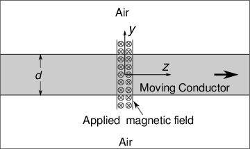
Figure 1: Schematic of the 2D problem.

In reference [21], 2D version of the moving conductor problem, which has adequate representation of the 3D problem, has been considered for evaluating the error at the interface. For the sake of completeness, a brief description of the 2D problem is provided here (see Fig. 1). An infinite conducting slab with thickness $d$ is placed between two air layers of thickness $4d$. The conductor has a uniform velocity $u_{z}$ along the $z-$axis and a localized $x$-directed magnetic field is considered. Boundary in the flow direction is introduced at $20d$ on either side of the magnetic field. The material properties of the slab are $\sigma=7.21\times 10^{6}Sm^{-1}$, $\mu_{r}=1$, $d=0.5m$. The FEM discretisation involved 5760 nodal, bilinear quadrilateral elements of rectangular shape. The element size is varied along the $y$-direction to accurately capture the currents circulating in the conductor. It can be noted that the 2D problem here represents the circulation of current and thus it consists of 2-components of vector potential $A_{y},A_{z}$.

The same 2D problem will be considered here for further analysis. In [21], it is shown that only SU/PG scheme suffers from boundary error and not the original Galerkin scheme or its variants [26]. In order to trace the genesis of this error numerically, computed results are analysed to detect the presence of any inconsistency.

         

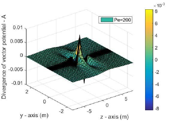
(a)

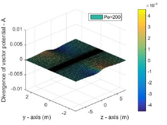
(b)

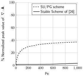
(c)

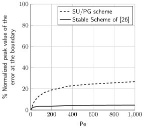
(d)

Figure 2: Selected results from the 2D problem. (a) $\nabla\cdot{\bf A}$ obtained from the SU/PG scheme (b) $\nabla\cdot{\bf A}$ obtained from Scheme presented in [26] (c) Peak values $\nabla\cdot{\bf A}$ over a range of $Pe$ obtained from SU/PG scheme and the stable scheme reported in [26]. (d) Peak values of the error over a range of $Pe$ as obtained from SU/PG scheme and the stable scheme reported in [26].

During the analysis, it is found that the use of Coulomb’s gauge i.e.,$\nabla\cdot{\bf A}=0$ condition, is being grossly violated in the SU/PG scheme, which is not the case with the GFEM based schemes. As an example, a sample result of $\nabla\cdot\bf A$ computed from the SU/PG scheme is presented in the Fig. 2a, where the presence of error could be clearly seen. Recently, a simple alternative scheme which is based on the classical GFEM has been presented in [26] and it is shown to be very stable. The computed $\nabla\cdot\bf A$ obtained by employing this scheme is also presented, in Fig. 2b.

In order to make a meaningful assessment, for each of the $Pe$, peak values of the $b_{x}$ is taken for normalisation. The required values are taken from the results presented in [21], which has been reproduced as Fig. 3c for a ready reference. By comparing the results, it can be seen that the value of error in $\nabla\cdot\bf A$ is about 30% in the SU/PG solution, while it is only about 5% for the scheme proposed in [26]. This suggests a method for a direct correlation between the transverse boundary error and the peak magnitude of $\nabla\cdot{\bf A}$. To get a more quantitative picture, both the peak error as well as the peak $\nabla\cdot{\bf A}$ are obtained for a range of $Pe$ and plotted in Figs. 2c and 2d. It is clear that the peak values of $\nabla\cdot{\bf A}$ and the peak boundary error with SU/PG scheme follows the exact same trend over the range of $Pe$.

This exercise clearly indicate that the boundary error in the solution is strongly correlated with the existence of $\nabla\cdot{\bf A}=0$ in the weak solution through SU/PG scheme. It is worth noting here that the Coulombs gauge is commonly employed in moving conductor literature [12, 13, 7, 27, 11] especially for the nodal formulation. The following vector identity is employed most of the times,

$$\nabla\times\nabla\times\bf A=\nabla(\nabla\cdot{\bf A})-\nabla^{2}\bf A$$ (3)

assuming $\nabla\cdot\bf A=0$,

$$\nabla\times\nabla\times\bf A=-\nabla^{2}\bf A$$ (4)

However, the results of SU/PG scheme does not confirm to $\nabla\cdot{\bf A}=0$ and therefore, it is necessary to avoid the use of Coulomb’s gauge (refer to Figs. 2a & 2c). For this the corresponding term must be retained in the formulation. Please note that this might result in non-unique value of $\bf A$, however, it is $\nabla\times{\bf A}$ is the variable of interest not $\bf A$ directly.

As the weak form for the Ampere’s law (which involves $\nabla\times\nabla\times{\bf{A}}$) is not readily available for scalar elements, it will be dealt below.

The weighted residue formulation for the $x$-component of $\nabla\times\dfrac{1}{\mu}\nabla\times\bf A$ is,

$$\int_{\Omega}N_{g}~{}(\nabla\times\dfrac{1}{\mu}\nabla\times{\bf A})\cdot\hat{\bf x}~{}d\Omega$$ (5)

where $N_{g}$ is the Galerkin weighting function and $\hat{\bf x}$ is the unit vector along the $x$-axis. Applying the vector identity given in (3) on (5),

$$\Rightarrow\int_{\Omega}N_{g}~{}\nabla\cdot\Big{(}\dfrac{1}{\mu}\dfrac{\partial{\bf A}}{\partial x}-\dfrac{1}{\mu}\nabla A_{x}\Big{)}~{}d\Omega$$ (6)

Applying integration by parts for (6),

$$\begin{split}\Rightarrow~{}-\int_{\Omega}~{}\nabla N_{g}\cdot\Big{(}\dfrac{1}{\mu}\dfrac{\partial{\bf A}}{\partial x}-\dfrac{1}{\mu}\nabla A_{x}\Big{)}~{}d\Omega~{}\dots{\\[8.53581pt] }+\oint_{\Gamma}N_{g}~{}\Big{(}\dfrac{1}{\mu}\dfrac{\partial{\bf A}}{\partial x}-\dfrac{1}{\mu}\nabla A_{x}\Big{)}\cdot\hat{\bf n}~{}d\Gamma\end{split}$$ (7)

where, $\hat{\bf n}$ is the unit normal vector. Remember that in the Laplacian formulation of scalar potential, by neglecting the boundary integral term in the weak form, the inter element boundary condition ${\bf D}_{1}\cdot{\hat{\bf n}}={\bf D}_{2}\cdot{\hat{\bf n}}$ or ${\bf J}_{1}\cdot{\hat{\bf n}}={\bf J}_{2}\cdot{\hat{\bf n}}$ get automatically satisfied [28]. Thus, it was not necessary to compute the boundary integral term there and that greatly improved the computational efficiency. Considering this, it is worthwhile to see the effect of neglecting the boundary integral term in the equation (7). The boundary integral term can be simplified as follows,

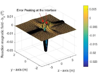
(a)

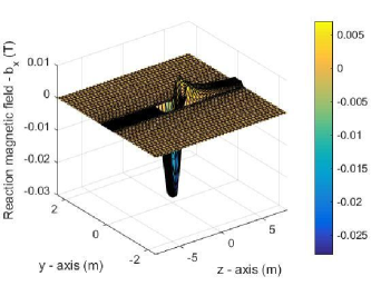
(b)

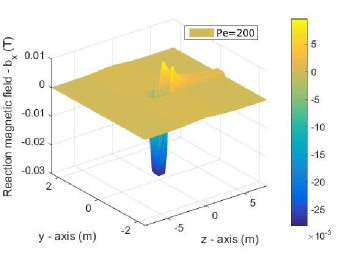
(c)

Figure 3: Reaction magnetic field $b_{x}$ obtained with the SU/PG scheme for $Pe=200$. (a) With the assumption of $\nabla\cdot{\bf A}=0$ (b) Without the assumption of $\nabla\cdot{\bf A}=0$ (c) Reference solution generated with very fine discretisation [21]

$$\begin{split}\Rightarrow~{}&\oint_{\Gamma}N_{g}~{}\Big{(}\dfrac{1}{\mu}\dfrac{\partial{\bf A}}{\partial x}-\dfrac{1}{\mu}\nabla A_{x}\Big{)}\cdot\hat{\bf n}~{}d\Gamma\\[5.69054pt] &=\oint_{\Gamma}\dfrac{N_{g}}{\mu}~{}\Big{(}\dfrac{\partial{A_{y}}}{\partial x}n_{y}+\dfrac{\partial{A_{z}}}{\partial x}n_{z}-\dfrac{\partial{A_{x}}}{\partial y}n_{y}-\dfrac{\partial{A_{x}}}{\partial z}n_{z}\Big{)}~{}d\Gamma\\[5.69054pt] &=\oint_{\Gamma}{N_{g}}~{}(h_{z}n_{y}-h_{y}n_{z})~{}d\Gamma\end{split}$$ (8)

where,

$$h_{z}=\dfrac{1}{\mu}\Big{(}\dfrac{\partial{A_{y}}}{\partial x}-\dfrac{\partial{A_{x}}}{\partial y}\Big{)}~{}~{}\text{and}~{}~{}h_{y}=\dfrac{1}{\mu}\Big{(}\dfrac{\partial{A_{x}}}{\partial z}-\dfrac{\partial{A_{z}}}{\partial x}\Big{)}$$

Equation (8) corresponds to the $x$-component, the boundary integral terms for other components can also be derived in the same fashion. The boundary integral term for the $y$-component is,

$$\oint_{\Gamma}{N_{g}}~{}(h_{x}n_{z}-h_{z}n_{x})~{}d\Gamma$$ (9)

and that for the $z$-component is,

$$\oint_{\Gamma}{N_{g}}~{}(h_{y}n_{x}-h_{x}n_{y})~{}d\Gamma$$ (10)

Combining (8), (9) and (10), the vector form of the boundary integral terms can be written as,

$$\Rightarrow~{}-\oint_{\Gamma}{N_{g}}~{}({\bf h}\times{\bf n})~{}d\Gamma$$ (11)

Equating (11) to zero results in maintaining the tangential continuity of the magnetic field intensity $\bf h$ [29], i.e.,

$$\bf h_{1}\cdot\hat{t}\approx h_{2}\cdot\hat{t}$$ (12)

across the elements 1 and 2. Thus, neglecting the boundary integral in (7), helps to maintain the continuity of magnetic field intensity across the element interface. Therefore, the weak formulation contains only the volume integral term in the proposed approach and the complete SU/PG-weak formulation of (1) and (2) are provided in the Appendix A.

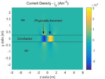
(a)

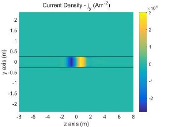
(b)

Figure 4: Current density $j_{y}=\partial h_{x}/\partial z$, obtained with the SU/PG scheme for $Pe=200$. (a) With the assumption of $\nabla\cdot{\bf A}=0$ (b) Without the assumption of $\nabla\cdot{\bf A}=0$

With this, the simulations are carried out for range of Peclet numbers and the sample simulation results are presented in Fig. 3. When the $\nabla\cdot{\bf{A}}$ is retained with the SU/PG scheme, error at the transverse boundary virtually disappears. Also, It can be clearly seen that the reaction magnetic field profile obtained with the proposed approach (Fig. 3b) is matching exactly with the reference solution presented in Fig. 3c. Consequently, the non-physical solution of $\nabla\times{\bf h}\neq 0$ in the adjacent air-region, is also seem to be practically absent with the proposed approach (refer to Fig. 4, which provides solution for both). For a range of $Pe$ considered in Fig. 2c, the simulation results with $\nabla\cdot{\bf A}$ retained is found to have peak error $<1\%$ (refer to Fig 5). In the next subsection, the effect of avoiding Coulomb’s gauge on the condition number of the FEM matrix is discussed.

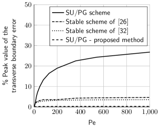
Figure 5: Comparison of % peak value of transverse boundary error present in different schemes

II-B Effect on condition number

TABLE I: Comparison of Condition number and accuracy

	SU/PG scheme with Proposed method (Node element)			Edge Element		SUPG Scheme (Node element)
Pe	$\alpha$	Condition no.	% Peak Error	Condition no.	% Peak Error	Condition no.	% Peak Error
	0.00	8.9415e+11	0.221
50	0.05	4.1364e+08	2.215	4.8747e+09	22.516	1.7352e+08	10.007
	0.10	3.2260e+08	3.466
	0.00	1.5178e+12	0.257
200	0.05	2.0991e+09	3.359	1.9438e+10	25.018	1.8165e+09	18.942
	0.10	1.9721e+09	5.361
	0.00	2.1925e+14	0.271
1000	0.05	4.0514e+11	4.289	3.3003e+11	25.733	1.8677e+11	30.021
	0.10	3.4614e+11	6.791

It is evident that the avoiding Coulomb’s gauge from the governing equation can impact the condition number of the final FEM matrix. In order to address this, a possible remedy is discussed in this subsection. In this, a scaled amount of $\nabla\cdot\bf{A}$ is injected into the original governing equation, with the scaling parameter $\alpha$. The results of this new variation is tabulated in Table I. For comparison, simulations also carried using the edge elements and the results of same is included in Table I. As mentioned in the introduction, the edge elements cannot inherently avoid the erroneous results arising out of the convection dominated simulations.

As shown in the table I, the % peak error in the proposed scheme can be seen to slowly increase as we increase the $\nabla\cdot\bf{A}$ contribution. However, for the values of $\alpha$ listed in the table, the accuracy of the proposed scheme is substantially better than the edge element method or the SU/PG scheme. When $\alpha=0.05$ or in other words, when the $\nabla\cdot\bf{A}$ addition is around 5%, the accuracy at the material interface is at least an order of magnitude better than the other methods; while keeping the condition number in a comparably reasonable value.

It can also be observed that the condition number from the edge element method is not better than the nodal element method. This may be attributed to the absence of normal continuity across the edge elements [30, 31].

II-C Verification with 3D electromagnetic flowmeter problem

As a demonstration of the efficacy of the proposed approach in real life situations, a practical 3D problem, the electromagnetic flowmeter, is simulated for high Peclet numbers. The simulation is carried out using the bilinear nodal elements. The simulation parameters and the input quantities are taken as mentioned in [26] and the schematic diagram of the electromagnetic flowmeter is shown in Fig. 6, with its $x,y,z-axes$ defined. The simulations are carried out for a range of Peclet numbers and the results are confirming the conclusions, which are drawn for the 2D problem. The sample simulation results are presented in Fig. 7, with $Pe=1600$. From Fig. 7a the non-physical current distribution in the air region can be seen, which is obtained from the SU/PG scheme, on the other hand, the retention of $\nabla\cdot\bf{A}$ in the SU/PG scheme provides a physically confirming solution (refer to Fig. 7b).

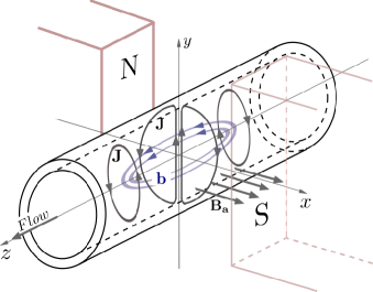
Figure 6: Schematic of the electromagnetic flowmeter, shown with the current density ${\bf J}$ and the reaction magnetic field ${\bf b}$

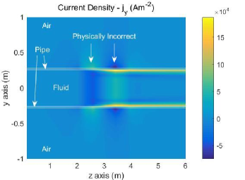
(a)

(b)

Figure 7: Current density $j_{y}=\partial h_{x}/\partial z-\partial h_{z}/\partial x$ in $x=0$ plane, obtained with the SU/PG scheme for $Pe=1600$. (a) With the assumption of $\nabla\cdot{\bf A}=0$ (b) Without the assumption of $\nabla\cdot{\bf A}=0$

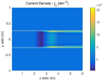
Figure 8: Current density $j_{y}=\partial h_{x}/\partial z-\partial h_{z}/\partial x$ in $x=0$ plane, obtained with the pole-zero cancellation based scheme [32] for $Pe=1600$.

Incidentally, the recent pole-zero cancellation based, stabilization schemes proposed in [26, 32] observed to give accurate solutions without the boundary error. A sample simulation result for $Pe=1600$ with the scheme proposed in [32], is provided in Fig. 8.

Referring to Fig. 6, along the $zy$-plane the complete circulation of induced current is represented. In the orthogonal direction, i.e., along the $zx$-plane the currents are orthogonal to the plane and they are mostly represented by the $y$-component of the current density $j_{y}$. The currents along the $zx$-plane does not get directly oriented by the boundary, unlike the circulation along the $zy$-plane. Owing to this, the boundary error is expected to be minimal along the $zx$-plane and the same is observed with this 3D simulation. To confirm this observation further, the 2D version of the moving conductor problem along the $zx$-plane is simulated. The results from this simulation indicate insignificant boundary error, along the $zx$-plane.

III Summary and Conclusion

The SU/PG scheme is widely adopted upwinding technique, for high flow velocity problems due to its simplicity and being void of crosswind of diffusion [33]. Besides, the transverse boundary error present in the SU/PG scheme is a serious issue and several non-linear solutions have been proposed (called as SOLD schemes) by the computational fluid dynamics community. Nevertheless, they suffer from computational inefficiency, as well as, some inaccuracy [24, 25]. In addition, these techniques are rarely employed for moving conductor problems.

In the present work, a 2D version of the moving conductor problem, is taken for the analysis. The 2D problem represents the complete circulation of current with in the conducting region and thus it consists of 2-components of vector potential. Here, the source of the transverse boundary error is identified with the enforcement of Coulomb gauge $\nabla\cdot{\bf A}=0$. Therefore, the $\nabla\cdot{\bf{A}}$ term is retained and the weak form of the Amperes’ law has been derived for scalar elements. Then, through the numerical simulation of 2D, as well as, 3D problems, it is shown that the retention of $\nabla\cdot{\bf{A}}$ practically eliminates the material interface boundary error present in the SU/PG scheme. In addition, this approach preserves the linearity, as well as, computational efficiency of the SU/PG scheme.

Appendix A Weak Form of the Governing Equations

The weak form of (2) can be commonly found in the computational electromagnetic literature. Nevertheless, for the sake of completeness and quick reference, it has been provided below, along with the weak form of (1), which is derived. The weak form of (2) can be written as,

$$\begin{split}\int_{\Omega}\sigma\nabla N_{g}\cdot\nabla\phi~{}d\Omega-\int_{\Omega}\sigma\nabla N_{g}\cdot({\bf u}\times\nabla\times{\bf{A}})~{}d\Omega~{}\dots{\\ }=\int_{\Omega}\sigma\nabla N_{g}\cdot({\bf u}\times{\bf B_{a}})~{}d\Omega\end{split}$$ (13)

The advection-diffusion form of (1) requires the modification of the Galerkin weighting function $N_{g}$ to the SU/PG weighting function $N_{s}$, which is given by,

$$N_{s}=N_{g}+\tau\dfrac{\Delta l~{}{\bf u}}{2\|{\bf u}\|}\cdot\nabla N_{g}$$ (14)

where $\tau$ is the stabilization parameter, defined as $\tau\equiv coth(|Pe|)-{1}/{|Pe|}$. The stabilization parameter $\tau$ decides the optimal (right) amount of upwinding which is being added to the Galerkin weight function $N_{g}$. This added term, is employed to only the element interiors and in case of linear elements, the second derivative vanishes and the modified weighting function $N_{s}$ is applied only to the advective/first derivative terms [34, 35, 33]. Therefore, the weak form of the $x$-component of (1) takes the form:

$$\begin{split}\int_{\Omega}\sigma N_{s}\dfrac{\partial\phi}{\partial x}~{}d\Omega~{}-\int_{\Omega}~{}\nabla N_{g}\cdot\Big{(}\dfrac{1}{\mu}\dfrac{\partial{\bf A}}{\partial x}-\dfrac{1}{\mu}\nabla A_{x}\Big{)}~{}d\Omega~{}\dots{\\[8.53581pt] }-\int_{\Omega}\sigma N_{s}~{}\Big{(}u_{y}\dfrac{\partial A_{y}}{\partial x}-u_{y}\dfrac{\partial A_{x}}{\partial y}-u_{z}\dfrac{\partial A_{x}}{\partial z}+u_{z}\dfrac{\partial A_{z}}{\partial x}\Big{)}~{}d\Omega~{}\dots{\\[8.53581pt] }+~{}\alpha\int_{\Omega}~{}\dfrac{\partial N_{g}}{\partial x}\nabla{\bf\cdot A}~{}d\Omega=\int_{\Omega}\sigma N_{s}(u_{y}B_{z}-u_{z}B_{y})~{}d\Omega\end{split}$$ (15)

and its $y$-component:

$$\begin{split}\int_{\Omega}\sigma N_{s}\dfrac{\partial\phi}{\partial y}~{}d\Omega~{}-\int_{\Omega}~{}\nabla N_{g}\cdot\Big{(}\dfrac{1}{\mu}\dfrac{\partial{\bf A}}{\partial y}-\dfrac{1}{\mu}\nabla A_{y}\Big{)}~{}d\Omega~{}\dots{\\[8.53581pt] }-\int_{\Omega}\sigma N_{s}~{}\Big{(}u_{z}\dfrac{\partial A_{z}}{\partial y}-u_{z}\dfrac{\partial A_{y}}{\partial z}-u_{x}\dfrac{\partial A_{y}}{\partial x}+u_{x}\dfrac{\partial A_{x}}{\partial y}\Big{)}~{}d\Omega~{}\dots{\\[8.53581pt] }+~{}\alpha\int_{\Omega}~{}\dfrac{\partial N_{g}}{\partial y}\nabla{\bf\cdot A}~{}d\Omega=\int_{\Omega}\sigma N_{s}(u_{z}B_{x}-u_{x}B_{z})~{}d\Omega\end{split}$$ (16)

and its $z$-component:

$$\begin{split}\int_{\Omega}\sigma N_{s}\dfrac{\partial\phi}{\partial z}~{}d\Omega~{}-\int_{\Omega}~{}\nabla N_{g}\cdot\Big{(}\dfrac{1}{\mu}\dfrac{\partial{\bf A}}{\partial z}-\dfrac{1}{\mu}\nabla A_{z}\Big{)}~{}d\Omega~{}\dots{\\[8.53581pt] }-\int_{\Omega}\sigma N_{s}~{}\Big{(}u_{x}\dfrac{\partial A_{x}}{\partial z}-u_{x}\dfrac{\partial A_{z}}{\partial x}-u_{y}\dfrac{\partial A_{z}}{\partial y}+u_{y}\dfrac{\partial A_{y}}{\partial z}\Big{)}~{}d\Omega~{}\dots{\\[8.53581pt] }+~{}\alpha\int_{\Omega}~{}\dfrac{\partial N_{g}}{\partial z}\nabla{\bf\cdot A}~{}d\Omega=\int_{\Omega}\sigma N_{s}(u_{x}B_{y}-u_{y}B_{x})~{}d\Omega\end{split}$$ (17)

For the 2D problem considered, the $x$-component of the equation vanishes and only the $y$ and $z$ components remain. Also, the velocity is assumed to be along the $z$ direction (${\bf u}=u_{z}{\bf\hat{z}}$) and the input magnetic field is $x$ directed (${\bf B_{a}}=B_{x}{\bf\hat{x}}$). With this, the weak forms of the governing equations (1) and (2) are respectively given by,

$$\begin{split}\int_{\Omega}\sigma N_{s}\dfrac{\partial\phi}{\partial y}~{}d\Omega~{}+\int_{\Omega}~{}\dfrac{1}{\mu}\Big{(}\dfrac{\partial N_{g}}{\partial z}\dfrac{\partial A_{y}}{\partial z}-\dfrac{\partial N_{g}}{\partial z}\dfrac{\partial A_{z}}{\partial y}\Big{)}~{}d\Omega~{}\dots{\\[8.53581pt] }+\int_{\Omega}\sigma N_{s}\Big{(}u_{z}\dfrac{\partial A_{y}}{\partial z}-u_{z}\dfrac{\partial A_{z}}{\partial y}\Big{)}~{}d\Omega~{}\dots{\\[8.53581pt] }+~{}\alpha\int_{\Omega}~{}\dfrac{\partial N_{g}}{\partial y}\Big{(}\dfrac{\partial A_{y}}{\partial y}+\dfrac{\partial A_{z}}{\partial z}\Big{)}~{}d\Omega=\int_{\Omega}\sigma N_{s}u_{z}B_{x}~{}d\Omega\end{split}$$ (18)

$$\begin{split}\int_{\Omega}\sigma N_{s}\dfrac{\partial\phi}{\partial z}~{}d\Omega~{}+\int_{\Omega}~{}\dfrac{1}{\mu}\Big{(}\dfrac{\partial N_{g}}{\partial y}\dfrac{\partial A_{z}}{\partial y}-\dfrac{\partial N_{g}}{\partial y}\dfrac{\partial A_{y}}{\partial z}\Big{)}~{}d\Omega~{}\dots{\\[8.53581pt] }+~{}\alpha\int_{\Omega}~{}\dfrac{\partial N_{g}}{\partial z}\Big{(}\dfrac{\partial A_{y}}{\partial y}+\dfrac{\partial A_{z}}{\partial z}\Big{)}~{}d\Omega=0\end{split}$$ (19)

$$\begin{split}\int_{\Omega}\sigma\Big{(}\dfrac{\partial N_{g}}{\partial y}\dfrac{\partial\phi}{\partial y}+\dfrac{\partial N_{g}}{\partial z}\dfrac{\partial\phi}{\partial z}\Big{)}~{}d\Omega+\int_{\Omega}\sigma u_{z}\dfrac{\partial N_{g}}{\partial y}\dfrac{\partial A_{y}}{\partial z}~{}d\Omega~{}\dots{\\[8.53581pt] }-\int_{\Omega}\sigma u_{z}\dfrac{\partial N_{g}}{\partial y}\dfrac{\partial A_{z}}{\partial y}~{}d\Omega=\int_{\Omega}\sigma u_{z}B_{x}\dfrac{\partial N_{g}}{\partial y}~{}d\Omega\end{split}$$ (20)

Sethupathy Subramanian received the bachelors degree in electrical and electronics engineering from Anna University, Chennai, India, in 2009. He received the masters and doctrate degrees in electrical engineering from Indian Institute of Science, Bangalore, India in 2011 and 2017 respectively. He is currently pursuing his graduate research at the Department of Physics, University of Notre Dame, USA. His research interests, pertinent to electrical engineering, include computational electromagnetics, numerical stability, finite element and edge element methods.

Udaya Kumar (Senior Member, IEEE) received the bachelor’s degree in electrical engineering from Bangalore University, Bangaluru, India, in 1989, and the M.E. and Ph.D. degrees in high-voltage engineering from the Indian Institute of Science, Bengaluru, India, in 1991 and 1998, respectively. He is currently a Professor with the High Voltage Laboratory, Department of Electrical Engineering, Indian Institute of Science. He is an Associate Editor of IEEE Transactions on Power Delivery & IET High Voltage.

Sujata Bhowmick received the B.E. degree in electrical engineering from IIEST, Shibpur, India, in 2006, and the M.E. degree in electrical engineering from the Indian Institute of Science, Bengaluru, India, in 2011. She received the Ph.D. degree from the Department of Electronic Systems Engineering, Indian Institute of Science, Bengaluru, India, in 2019. Her current research interests include power electronics for renewable resources, single-phase grid-connected power converters, computational electromagnetics, finite element and edge element methods.

References

- [1] O. Biro, K. Preis, W. Renhart, K. Richter, and G. Vrisk, “Performance of different vector potential formulations in solving multiply connected 3-d eddy current problems,” IEEE Trans. Magnetics, vol. 26, no. 2, pp. 438–441, 1990.
- [2] T. Shimizu, N. Takeshima, and N. Jimbo, “A numerical study on faraday-type electromagnetic flowmeter in liquid metal system, (i),” Journal of Nuclear Science and Technology, vol. 37, no. 12, pp. 1038–1048, 2000.
- [3] O. Zienkiewicz, R. Taylor, and P. Nithiarasu, The Finite Element Method for Fluid Dynamics. Elsevier Science, 2005.
- [4] D. Spalding, “A novel finite difference formulation for differential expressions involving both first and second derivatives,” International Journal for Numerical Methods in Engineering, vol. 4, no. 4, pp. 551–559, 1972.
- [5] A. Runchal, “Convergence and accuracy of three finite difference schemes for a two-dimensional conduction and convection problem,” International Journal for Numerical Methods in Engineering, vol. 4, no. 4, pp. 541–550, 1972.
- [6] I. Christie, D. F. Griffiths, A. R. Mitchell, and O. C. Zienkiewicz, “Finite element methods for second order differential equations with significant first derivatives,” International Journal for Numerical Methods in Engineering, vol. 10, no. 6, pp. 1389–1396, 1976.
- [7] M. Odamura, “Upwind finite element solution for saturated traveling magnetic field problems,” Electrical Engineering in Japan, vol. 105, no. 4, pp. 126–132, 1985.
- [8] M. Ito, T. Takahashi, and M. Odamura, “Up-wind finite element solution of travelling magnetic field problems,” IEEE Trans. Magnetics, vol. 28, no. 2, pp. 1605–1610, 1992.
- [9] D. Rodger, P. Leonard, and T. Karaguler, “An optimal formulation for 3d moving conductor eddy current problems with smooth rotors,” IEEE Trans. Magnetics, vol. 26, no. 5, pp. 2359–2363, 1990.
- [10] E. Chan and S. Williamson, “Factors influencing the need for upwinding in two-dimensional field calculation,” IEEE Trans. Magnetics, vol. 28, no. 2, pp. 1611–1614, 1992.
- [11] N. Allen, D. Rodger, P. Coles, S. Strret, and P. Leonard, “Towards increased speed computations in 3d moving eddy current finite element modelling,” IEEE Trans. Magnetics, vol. 31, no. 6, pp. 3524–3526, 1995.
- [12] D. Rodger, T. Karguler, and P. Leonard, “A formulation for 3d moving conductor eddy current problems,” IEEE Trans. Magnetics, vol. 25, no. 5, pp. 4147–4149, 1989.
- [13] J. Bird, T. Lipo et al., “A 3-d magnetic charge finite-element model of an electrodynamic wheel,” IEEE Trans. Magnetics, vol. 44, no. 2, pp. 253–265, 2008.
- [14] H. Vande Sande, H. De Gersem, and K. Hameyer, “Finite element stabilization techniques for convection-diffusion problems,” 7th International journal of theoretical electrotechnics, pp. 56–59, 1999.
- [15] L. Codecasa and P. Alotto, “2-d stabilized fit formulation for eddy-current problems in moving conductors,” IEEE Trans. Magnetics, vol. 51, no. 3, pp. 1–4, 2015.
- [16] Y. Liang, “Steady-state thermal analysis of power cable systems in ducts using streamline-upwind/petrov-galerkin finite element method,” Dielectrics and Electrical Insulation, IEEE Transactions on, vol. 19, no. 1, pp. 283–290, 2012.
- [17] S. Noguchi and S. Kim, “Magnetic field and fluid flow computation of plural kinds of magnetic particles for magnetic separation,” IEEE Trans. Magnetics, vol. 48, no. 2, pp. 523–526, 2012.
- [18] E. X. Xu, J. Simkin, and S. C. Taylor, “Streamline upwinding in a 3-d edge-element method modeling eddy currents in moving conductors,” IEEE transactions on magnetics, vol. 42, no. 4, pp. 667–670, 2006.
- [19] F. Henrotte, H. Heumann, E. Lange, and K. Hameyer, “Upwind 3-d vector potential formulation for electromagnetic braking simulations,” IEEE Transactions on Magnetics, vol. 46, no. 8, pp. 2835–2838, 2010.
- [20] T. J. Hughes, M. Mallet, and M. Akira, “A new finite element formulation for computational fluid dynamics: Ii. beyond supg,” Computer Methods in Applied Mechanics and Engineering, vol. 54, no. 3, pp. 341–355, 1986.
- [21] S. Subramanian and U. Kumar, “Existence of boundary error transverse to the velocity in su/pg solution of moving conductor problem,” in Numerical Electromagnetic and Multiphysics Modeling and Optimization (NEMO), 2016 IEEE MTT-S International Conference on. IEEE, 2016, pp. 1–2.
- [22] R. Codina, “A discontinuity-capturing crosswind-dissipation for the finite element solution of the convection-diffusion equation,” Computer Methods in Applied Mechanics and Engineering, vol. 110, no. 3, pp. 325–342, 1993.
- [23] E. Oñate, F. Zárate, and S. R. Idelsohn, “Finite element formulation for convective–diffusive problems with sharp gradients using finite calculus,” Computer methods in applied mechanics and engineering, vol. 195, no. 13, pp. 1793–1825, 2006.
- [24] V. John and P. Knobloch, “On spurious oscillations at layers diminishing (sold) methods for convection–diffusion equations: Part i–a review,” Computer Methods in Applied Mechanics and Engineering, vol. 196, no. 17, pp. 2197–2215, 2007.
- [25] ——, “On spurious oscillations at layers diminishing (sold) methods for convection–diffusion equations: Part ii–analysis for p1 and q1 finite elements,” Computer Methods in Applied Mechanics and Engineering, vol. 197, no. 21, pp. 1997–2014, 2008.
- [26] S. Subramanian and U. Kumar, “Augmenting numerical stability of the galerkin finite element formulation for electromagnetic flowmeter analysis,” IET Science, Measurement & Technology, vol. 10, no. 4, pp. 288–295, 2016.
- [27] S.-K. Hong and N. Ida, “Modeling of velocity terms in 3d eddy current problems,” IEEE Trans. Magnetics, vol. 28, no. 2, pp. 1178–1181, 1992.
- [28] J. Shercliff, The Theory of Electromagnetic Flow-Measurement, ser. Cambridge Science Classics. Cambridge University Press, 1987.
- [29] P. P. Silvester and R. L. Ferrari, Finite elements for electrical engineers. Cambridge university press, 1996.
- [30] G. Mur, “Edge elements, their advantages and their disadvantages,” IEEE transactions on magnetics, vol. 30, no. 5, pp. 3552–3557, 1994.
- [31] ——, “The fallacy of edge elements,” IEEE Transactions on Magnetics, vol. 34, no. 5, pp. 3244–3247, 1998.
- [32] S. Subramanian and U. Kumar, “Stable galerkin finite-element scheme for the simulation of problems involving conductors moving rectilinearly in magnetic fields,” IET Science, Measurement & Technology, vol. 10, no. 8, pp. 952–962, 2016.
- [33] T.-P. Fries and H. G. Matthies, “A review of petrov–galerkin stabilization approaches and an extension to meshfree methods,” Technische Universitat Braunschweig, Brunswick, 2004.
- [34] T. J. Hughes, “Multiscale phenomena: Green’s functions, the dirichlet-to-neumann formulation, subgrid scale models, bubbles and the origins of stabilized methods,” Computer methods in applied mechanics and engineering, vol. 127, no. 1, pp. 387–401, 1995.
- [35] A. N. Brooks and T. J. Hughes, “Streamline upwind/petrov-galerkin formulations for convection dominated flows with particular emphasis on the incompressible navier-stokes equations,” Computer methods in applied mechanics and engineering, vol. 32, no. 1, pp. 199–259, 1982.