SLAW: Scaled Loss Approximate Weighting for Efficient Multi-Task Learning

Abstract

Multi-task learning (MTL) is a subfield of machine learning with important applications, but the multi-objective nature of optimization in MTL leads to difficulties in balancing training between tasks. The best MTL optimization methods require individually computing the gradient of each task’s loss function, which impedes scalability to a large number of tasks. In this paper, we propose Scaled Loss Approximate Weighting (SLAW), a method for multi-task optimization that matches the performance of the best existing methods while being much more efficient. SLAW balances learning between tasks by estimating the magnitudes of each task’s gradient without performing any extra backward passes. We provide theoretical and empirical justification for SLAW’s estimation of gradient magnitudes. Experimental results on non-linear regression, multi-task computer vision, and virtual screening for drug discovery demonstrate that SLAW is significantly more efficient than strong baselines without sacrificing performance and applicable to a diverse range of domains.

1 Introduction

As machine learning models become more powerful, they gain the ability to perform tasks which were previously thought impossible. With a growing pool of potential tasks, it is less feasible to obtain a labeled dataset and train a model from scratch for each new task. Multi-task learning (MTL) [3] can alleviate this scalability issue by training models to perform multiple tasks simultaneously, sharing parameters and supervision. Along with increased data and compute efficiency, knowledge sharing can create an implicit regularization which leads to performance improvements over single-task models [36].

Unfortunately, achieving this boost in efficiency and performance through MTL isn’t easy, due to the fact that multi-task optimization requires optimizing several (potentially competing) objectives. Previous methods have been proposed to ease the difficulties of multi-task optimization by balancing learning between tasks [18, 5, 22, 42] or addressing negative transfer [38, 21], where learning on one task hinders learning on another.

The best performing of these recent methods, such as GradNorm [5], PCGrad [38], and IMTL [21] compute the gradients of each individual task’s loss function, which requires one additional backwards pass per task for each training step. Even when these methods are sped up by only computing gradients for a subset of network weights, scalability to a large number of tasks is still an issue, since the number of required gradient computations scales linearly with the number of tasks.

To address this issue of scalability, we introduce Scaled Loss Approximate Weighting (SLAW), an efficient method for multi-task optimization that can be applied in any gradient-based multi-task learning setting. Instead of computing task-specific gradients, SLAW balances learning between tasks by assigning weight to tasks based on the estimated magnitude of each task’s gradient. This estimation is theoretically and empirically justified, and by shedding the need to directly compute gradients of each task’s loss function, SLAW is faster than existing methods and better able to scale to a large number of tasks. We also show that SLAW is closely related to existing optimization methods. In particular, we demonstrate that SLAW directly estimates a solution to a special case of the optimization problem iteratively solved by GradNorm [5].

Our experiments show that SLAW performs as well or better than existing methods while being much more efficient. For a collection of 10 non-linear regression tasks, SLAW converges to the ideal optimization trade-off between tasks. For joint semantic segmentation, surface normal estimation, and depth prediction on NYUv2 [27], SLAW performs as well or better than GradNorm and PCGrad while running about twice as fast. Finally, for a collection of 128 virtual screening tasks for drug discovery with the PubChem BioAssay (PCBA) dataset [37], SLAW runs 24.4 times faster than GradNorm and 33.0 times faster than PCGrad, while outperforming GradNorm and being competitive with PCGrad.

Our contributions can be summarized as follows:

• We propose Scaled Loss Approximate Weighting (SLAW), an efficient, simple, and general method for multi-task optimization. Unlike existing methods, SLAW does not compute the gradient of each task’s loss function, which greatly reduces computational cost.

• We provide theoretical and empirical justification for SLAW’s estimation of the magnitudes of task-specific gradients, demonstrating that SLAW can accurately balance learning between tasks without performing additional backwards passes.

• We analyze the relationship between SLAW and existing methods. In particular, we show that SLAW directly estimates a solution to a special case of the optimization problem that GradNorm [5] iteratively solves to balance learning between tasks.

• We provide experiments on a collection of non-linear regression tasks, NYUv2 [27], and a collection of virtual screening tasks from PCBA [37] showing that SLAW quickly learns ideal loss weights, has strong overall performance, exhibits efficiency and scalability to a large number of tasks, and is applicable to many different domains.

The rest of this paper is structured as follows. In Section 2, we review work related to ours. Section 3 provides background, a derivation of SLAW, and an analysis of SLAW’s relationship with existing methods. We present experimental evaluations in Section 4, and conclude with Section 5.

2 Related Work

Multi-task learning [3] has a long history both within and outside of deep learning. MTL eases deep learning’s need for huge amounts of training data and to start learning each new task from scratch. Training shared parameters on multiple tasks allows for supervision of one task to aid in the learning for another, and a set of trained shared features can often be reused to instantiate learning on a new task, yielding faster learning through feature reuse [28]. However, achieving increased data efficiency, transfer robustness, and regularization from MTL is never guaranteed and highly dependent on the relationships between the tasks involved [36, 2].

Many families of methods for MTL have arisen, including multi-task architectures [26, 34, 29, 24], optimization strategies [11, 4, 18, 38], and methods for learning task relationships [2, 39, 36, 1]. In this paper, we focus on optimization. Weighting by Uncertainty [18] treats loss weights as learnable parameters that model the uncertainty for each task. GradNorm [5] also treats the weights as learnable parameters, but the weights are optimized separately from network parameters to encourage ideal magnitudes of each task loss’s gradient. Dynamic Weight Averaging [22] (or DWA) was introduced as a computationally efficient alternative to GradNorm that doesn’t deal with individual task gradients. Recently, methods like PCGrad [38] and Impartial MTL [21] balance learning across tasks by considering the relationships between directions of gradients of each task’s loss function. For a review of MTL as a whole, see [40, 8].

MTL has been applied in many domains, such as computer vision [26], natural language processing [7], reinforcement learning [29], bioinformatics [31], and more. Of these domains, this paper applies MTL to computer vision and bioinformatics. Computer vision lends itself well to MTL since many tasks rely on common visual features. Earlier works [41, 12, 9] focus on training a shared feature extractor jointly on many tasks. Other architectures leverage task-specific networks with information flow between networks, such as Cross-Stitch Networks [26], Sluice Networks [34], and NDDR-CNN [14]. Bioinformatics has historically been less popular as an application domain for MTL researchers, though there are some examples, most notably [31]. [6] and [25] provide surveys of deep learning for biology and healthcare.

3 Methods

3.1 Background

In the usual formulation of machine learning, a parameterized model $f_{\theta}$ is trained to approximate a target function by finding a value of $\theta$ which minimizes a loss function $L(\theta)$. In contrast, MTL involves training multiple parameterized models that share parameters on multiple tasks; $f_{1,\theta},f_{2,\theta},...,f_{n,\theta}$ are jointly trained by minimizing a sum of loss functions $\sum_{i=1}^{n}w_{i}L_{i}(\theta)$. Here $L_{i}$ is a loss function for task $i$ and the coefficients $w_{i}$ are called loss weights, traditionally hand-picked to control the optimization trade-off between various task losses. Parameter sharing across tasks decreases memory cost, and multi-task models may outperform their single-task counterparts. However, there is no guarantee of this perfomance boost.

Although the coefficients $w_{i}$ in the MTL loss are traditionally hand-picked, these loss weights can also be chosen algorithmically to ease multi-task optimization. Several methods have been proposed to automatically choose loss weights based on task uncertainty [18], learning speed [5, 22, 42, 23], and task performance [15].

Previous work [5] pointed out that loss weighting can serve to balance the norms of each task loss’s gradient. Specifically, let $g_{i}=\nabla L_{i}(\theta)$. If the task loss functions $L_{i}$ are such that the norms of the task gradients $\|g_{i}\|$ are varying in their magnitude, then the tasks with large $\|g_{i}\|$ will dominate the training process. In this case, some tasks are “left behind” and not trained adequately. To offset this, loss weights can be chosen so that the weighted task gradient norms $w_{i}\|g_{i}\|$ have similar magnitudes, resulting in all tasks being trained equally.

3.2 Scaled Loss Approximate Weighting

In this section, we derive our algorithm for multi-task optimization: Scaled Loss Approximate Weighting (SLAW). SLAW is motivated by the idea that loss weighting in MTL can balance the norms of task loss gradients. However, SLAW does so without explicitly computing the gradient of each task’s loss, significantly improving on the scalability and efficiency of recent methods without sacrificing performance. In the following, we omit the dependence of $L_{i}$ and $f_{i}$ on $\theta$ for convenience of notation.

The goal of SLAW is to choose loss weights $w_{i}$ so that the weighted gradient norms of each task loss are equal:

$$w_{i}\|g_{i}\|=w_{j}\|g_{j}\|~{}\forall i,j$$ (1)

If we treat each $w_{i}$ as unknown and each $\|g_{i}\|$ as known, then Equation 1 yields a homogeneous linear system of $n-1$ equations with $n$ unknowns, so that there are infinitely many solutions of $w_{i}$. One such solution is:

$$w_{i}=\frac{1}{\|g_{i}\|}$$ (2)

Following previous works [5, 22], we also decouple the global learning rate from the loss weights $w_{i}$ by enforcing a constraint on the sum of the loss weights:

$$\sum_{i=1}^{n}w_{i}=n$$ (3)

So that the mean value of $w_{i}$ is 1. Adding Equation 3 to our system of equations from Equation 1, we obtain a homogeneous linear system of $n$ equations with $n$ unknowns. Combining Equations 2 and 3, we can see that the following values of $w_{i}$ are a valid solution to this system:

$$w_{i}=\frac{n}{\|g_{i}\|}\bigg{/}\sum_{j=1}^{n}\frac{1}{\|g_{j}\|}$$ (4)

Setting the loss weights in this way at each training step would satisfy the equal gradient condition in Equation 1 as well as the temperature condition in Equation 3, balancing the task gradients as originally desired. However, this would require computing the gradient $g_{i}$ of each task’s loss function.

To avoid this computational cost, we can approximate the RHS of Equation 4 by approximating the values of each $\|g_{i}\|$. Notice that Equation 4 only depends on the magnitude of each task’s gradient, so that an approximation of $\|g_{i}\|$ is sufficient to approximate Equation 4. The following theorem gives a method for such an approximation:

Theorem 1.

Let $f:\mathbb{R}^{d}\rightarrow\mathbb{R}$ be continuously differentiable and Lipschitz continuous with Lipschitz constant $K$. Then for any $\mathbf{x}_{0}\in\mathbb{R}^{d}$ and $\epsilon>0$, there exists $\delta>0$ and constants $K_{1},K_{2}$ (which depend only on $n$, $K$, $\delta$, and $\epsilon$) so that:

$$\left|\text{Var}[f(\mathbf{X})]-(K_{1}\|\nabla f(\mathbf{x}_{0})\|^{2}+K_{2})\right|<\epsilon$$ (5)

where $\mathbf{X}$ is a random variable which is uniformly distributed over $\{\mathbf{x}_{0}+\mathbf{d}:\|\mathbf{d}\|<\delta\}$.

The proof is given in Appendix A. Put simply, this theorem tells us that the standard deviation of a “well-behaved” function in a neighborhood around a point is nearly proportional to the norm of the gradient at that point. If we assume that the task loss functions $\{L_{i}\}_{i=1}^{n}$ are continuously differentiable and Lipschitz continuous (a relatively weak assumption), then we can conclude that the norm of the task gradient $\|g_{i}\|$ at a point $\theta_{0}$ is proportional to the standard deviation of loss values $L_{i}(\theta)$ as $\theta$ varies in a neighborhood around $\theta_{0}$. Proportional, in this case, is sufficient. We only need to compute the relative magnitudes of the task gradients in order to approximate Equation 4, since the loss weights $w_{i}$ are linearly scaled to fit Equation 3.

To implement the approximation described by Theorem 1, we simply keep a running estimate of the standard deviation of $L_{i}$ through consecutive training steps. Treating each $L_{i}$ as a random variable, we compute an exponential moving average of the first and second moments of $L_{i}$, and use this to approximate the standard deviation of $L_{i}$:

$$a_{i} \leftarrow\beta a_{i}+(1-\beta)L_{i}^{2},$$ (6)

$$b_{i} \leftarrow\beta b_{i}+(1-\beta)L_{i},$$ (7)

$$s_{i} \leftarrow\sqrt{a_{i}-b_{i}^{2}},$$ (8)

where $\beta$ is a parameter of the moving average. Since $s_{i}$ estimates the standard deviation of $L_{i}$, by Theorem 1, $s_{i}$ is nearly proportional to $\|g_{i}\|$. We can then use $s_{i}$ as an approximation to $\|g_{i}\|$ in Equation 4, which gives us SLAW:

$$w_{i}=\frac{n}{s_{i}}\bigg{/}\sum_{j=1}^{n}\frac{1}{s_{j}}$$ (9)

In the full algorithm, shown in Algorithm 1, we replace $s_{i}$ with $\max(s_{i},10^{-5})$ for numerical stability. The only hyperparameter of SLAW is the moving average coefficient $\beta$.

Algorithm 1 Scaled Loss Approximate Weighting

  $\theta\leftarrow$ initialize()

  $w_{i}\leftarrow 1.0$ for $i=1$ to $n$

  $a_{i},b_{i},s_{i}\leftarrow 0.0$ for $i=1$ to $n$

  for $t=0,1,2,...$ do

     $x\leftarrow$ sample_batch()

     $L_{1},L_{2},...,L_{n}\leftarrow$ forward($x$)

     $a_{i}\leftarrow\beta a_{i}+(1-\beta)L_{i}$ for $i=1$ to $n$

     $b_{i}\leftarrow\beta b_{i}+(1-\beta)L_{i}^{2}$ for $i=1$ to $n$

     $s_{i}\leftarrow\max(\sqrt{a_{i}-b_{i}^{2}},10^{-5})$ for $i=1$ to $n$

     $w_{i}\leftarrow\frac{n}{s_{i}}/\sum_{j=1}^{n}\frac{1}{s_{j}}$ for $i=1$ to $n$

     $L\leftarrow\sum_{i=1}^{n}w_{i}L_{i}$

     $\theta\leftarrow$ update($\theta,L$)

  end for

Lastly, it should be noted that the approximation of $\|g_{i}\|$ by $s_{i}$ in SLAW does not exactly match the conditions specified by Theorem 1. Theorem 1 says that we can approximate the norm of a function’s gradient at a given point by measuring the standard deviation of that function in a neighborhood around that point. In SLAW, we approximate the gradients of task losses by measuring the standard deviation of each task loss not in a neighborhood around the current $\theta$, but over recent values of $\theta$ during training. However, an empirical comparison shows that SLAW’s estimates of task gradient norms are still reasonably proportional to the true gradient norm during training (see Appendix B for details).

3.3 Relation to Existing Methods

SLAW has a strong relationship with GradNorm [5], Dynamic Weight Averaging [22], and Adam [19]. We discuss their similarities and differences below.

GradNorm [5] is a well-known method for loss weighting in MTL with a similar motivation as SLAW: to balance the norms of the gradients of each task’s loss function. GradNorm learns loss weights $w_{i}$ by minimizing the distance from the weighted gradient norms to target values. Specifically, for task gradients $g_{i}=\nabla L_{i}$, let $G=\frac{1}{n}\sum_{i=1}^{n}\|g_{i}\|$, let $\tilde{L}_{i}=L_{i}/L_{0i}$, where $L_{0i}$ is the loss of the $i$-th task on the first step of training, and let $r_{i}=\tilde{L}_{i}\big{/}\frac{1}{n}\sum_{j=1}^{n}\tilde{L}_{j}$. The GradNorm loss weights $w_{i}$ are learned by minimizing the following loss function:

$$L_{\text{grad}}(\{w_{i}\}_{i=1}^{n})=\sum_{i=1}^{n}|w_{i}\|g_{i}\|-Gr_{i}^{\alpha}|$$ (10)

where $\alpha$ is a hyperparameter that controls the degree to which the magnitude of gradients from different tasks may differ under GradNorm. After each optimization step, the loss weights are scaled so that their average value is 1.

On the surface, the GradNorm algorithm doesn’t bear much resemblance to SLAW. We can gain insight into the relationship between these two algorithms by directly computing the global minimum of $L_{\text{grad}}$. We know that $L_{\text{grad}}\geq 0$, since $L_{\text{grad}}$ is a sum of absolute values. We can achieve $L_{\text{grad}}=0$ with the following values of $w_{i}$:

$$w_{i}=\frac{Gr_{i}^{\alpha}}{\|g_{i}\|}$$ (11)

Further, these are the only loss weights with $L_{\text{grad}}=0$. Therefore, Equation 11 gives a unique minimizer of $L_{\text{grad}}$. Scaling these weights so that their average value is 1, we see that GradNorm’s optimal loss weights are:

$$w_{i} =n\frac{r_{i}^{\alpha}}{\|g_{i}\|}\bigg{/}\sum_{j=1}^{n}\frac{r_{j}^{\alpha}}{\|g_{j}\|}$$ (12)

In the case where $\alpha=0$, where weights are learned so that all tasks have equal gradient norms, this becomes:

$$w_{i}=\frac{n}{\|g_{i}\|}\bigg{/}\sum_{j=1}^{n}\frac{1}{\|g_{j}\|}$$ (13)

In summary, Equation 13 describes the global minimizer of $L_{\text{grad}}$ in the case that $\alpha=0$. However, Equation 13 is the exact same as Equation 4, which is approximated by SLAW. Therefore, SLAW approximates the global solution to the GradNorm loss weight optimization problem for the case that $\alpha=0$. SLAW does this without computing the task-specific gradients $g_{i}$, greatly reducing computational cost.

Dynamic Weight Averaging [22] was introduced as a simpler and faster alternative to GradNorm, similarly to SLAW. It works by assigning more weight to tasks for which learning is slow. The learning speed of a task is defined as the ratio of that task’s loss function on recent training steps: $L_{i}(t-1)/L_{i}(t-2)$. DWA is efficient: it does not require individual task gradients.

However, our experiments show that DWA does not learn meaningful loss weights. For a variety of tasks and architectures, we found that each loss weight $w_{i}$ learned by DWA oscillates around 1.0. DWA isn’t theoretically justified, and the empirical results from [22] do not show that DWA outperforms the naive constant weight method with statistical significance. Our theoretical and empirical evidence shows that SLAW provides what DWA does not: an efficient, effective alternative to GradNorm.

Adam [19] is a widely-used stochastic optimization method. Adam, like SLAW, keeps estimates of gradient statistics that are used to normalize model updates:

$$\theta\leftarrow\theta-\eta\cdot\hat{m}_{t}/(\sqrt{\hat{v}_{t}}+\epsilon)$$ (14)

where $\eta$ is the learning rate, $\epsilon$ is a small constant included for numerical stability, and $\hat{m}_{t}$ and $\hat{v}_{t}$ are running estimates of the first and second moments, respectively, of the gradient of the function being optimized. Adam’s scaling of the update by a factor of $1/(\sqrt{\hat{v}_{t}}+\epsilon)$ is very similar to SLAW’s, which approximately scales the update from each loss function $L_{i}$ by a factor of $1/\|g_{i}\|$ (before normalization of $w_{i}$).

The key difference between Adam and SLAW is the fact that SLAW scales task loss functions, whereas Adam scales updates for each model parameter. These two normalizations have independent effects: SLAW balances training of the entire model across tasks, while Adam balances training on the aggregate MTL task across parameters.

4 Experiments

With our experiments, we seek to answer the following questions: (1) How accurately and quickly do loss weights learned by SLAW converge to the ideal loss weights compared to existing methods? (2) How does the performance of multi-task networks trained with SLAW compare to that of existing methods? (3) How does SLAW’s running time compare to that of existing methods?

We investigate each one of these questions by evaluating SLAW and various baselines on a different application domain. To evaluate loss weight quality, we use a set of non-linear regression tasks proposed in [5], where the ideal loss weights are known. We refer to this collection of tasks as MTRegression. For overall performance, we train jointly on semantic segmentation, surface normal estimation, and depth prediction on the NYUv2 dataset [27]. Finally, to evaluate the efficiency of SLAW relative to other methods, we train models on a number of virtual screening tasks varying from 32 to 128 on the PubChem BioAssay (PCBA) dataset [37].

In these investigations, we compare SLAW against the following multi-task baselines:

• Constant: The naive loss weighting method, where $w_{i}=1$ for all $i$.

• IdealConstant: Only used for MTRegression. Constant weight values of $w_{i}=1/\sigma_{i}^{2}$, so that each loss function is perfectly balanced. This is used as an upper bound on the performance of the other baselines.

• Weighting by Uncertainty [18]: The loss weights $w_{i}$ are treated as learnable parameters which are trained jointly with model parameters $\theta$. The loss function is derived from a probabilistic formulation of classification and regression problems.

• GradNorm [5]: Loss weights are learned by solving an optimization problem to balance the norm of task gradients. Details are given in Section 3.3.

• Dynamic Weight Averaging [22]: DWA sets loss weights $w_{i}$ so that tasks for which learning has been slow will receive more weight.

• PCGrad [38]: PCGrad computes the gradients for each task loss and modifies them to avoid pairwise conflicts without explicitly computing loss weights.

Experiments were run in a unified codebase containing our own implementations of Weighting by Uncertainty, GradNorm, DWA, PCGrad, and SLAW. Our GradNorm implementation computes task-specific gradients only for the last shared layer of the network, following the original work [5]. The unified code ensures a fair comparison between methods, and the code is publicly available for transparency and reproducibility. Experiments were run on a single NVIDIA RTX 3090.

4.1 Loss Weight Quality (MTRegression)

Training Settings

[5] introduces a collection of $n$ synthetic non-linear regression tasks defined by the following functions:

$$f_{i}(\mathbf{x})=\sigma_{i}\tanh((B+\epsilon_{i})\mathbf{x})$$ (15)

where the matrix $B$ is shared between all tasks, while $\sigma_{i}$ and $\epsilon_{i}$ are specific to each task. We refer to this collection of tasks as MTRegression. The task is defined so that loss functions of various tasks have significantly different scale, posing a testbed for multi-task optimization. The input and output dimensions are 250 and 100, respectively, and the elements of $B$ and $\epsilon_{i}$ are sampled independently from $\mathcal{N}(0,10)$ and $\mathcal{N}(0,3.5)$, respectively. In our experiments, we set $\sigma_{i}=i$ and $n=10$. The dataset has 9000 training samples and 1000 testing samples, where each sample has an input value and a label for each of the $n$ tasks.

Following [5], we train a fully connected network made of a shared trunk with 4 fully-connected layers, ReLU activations, and a hidden size of 100, followed by $n$ one-layer task-specific output heads that produce the prediction for each task. Each task’s loss function is a standard squared error between model output and ground-truth. In each experiment the network is trained to minimize the weighted sum of the $n$ task losses: $\sum_{i=1}^{n}w_{i}L_{i}$, where $w_{i}$ is determined differently by each method evaluated.

We run training for 300 epochs with a batch size of 304, following the table of hyperparameters in Appendix C. For each method, we run 10 training runs with different random seeds and report the average metric values over all runs.

We evaluate both the model performance and the quality of learned loss weights for each method considered. Since the task loss functions $L_{i}$ are artificially scaled by a factor of $\sigma_{i}^{2}$, the ideal value of each $w_{i}$ to balance the magnitude of task loss functions is $w_{i}=1/\sigma_{i}^{2}$. Using this information, we define a loss weight error of a set of loss weights $\{w_{i}\}_{i=1}^{n}$ as the mean squared error from $\{w_{i}\}_{i=1}^{n}$ to the ideal weights. To evaluate performance on MTRegression, we follow [5] and compute a normalized loss that considers all tasks equally: the mean of loss functions $L_{i}$ scaled by a factor of $1/\sigma_{i}^{2}$.

	Train NL	Test NL
Constant	$13.036\pm 0.032$	$13.635\pm 0.035$
IdealConstant	$\mathbf{11.744}\pm 0.033$	$\mathbf{12.274}\pm 0.035$
Uncertainty	-	-
GradNorm	$11.955\pm 0.039$	$12.509\pm 0.041$
DWA	$13.036\pm 0.032$	$13.635\pm 0.035$
PCGrad	$12.986\pm 0.037$	$13.581\pm 0.042$
SLAW (Ours)	$\mathbf{11.762}\pm 0.034$	$\mathbf{12.294}\pm 0.046$

Table 1: Final normalized loss (NL) for various methods on MTRegression, averaged over 10 training runs and with 95% confidence intervals. Best results for training and testing are bolded. Uncertainty [18] exhibited training instability.

Results

Figure 1 shows the loss weight error of each method throughout training, averaged over 10 training runs, and the normalized losses achieved at the end of training are shown in Table 1. The loss weight error is only plotted for the first 2000 of 9900 training steps in order to better visualize the differences between methods, since the loss weight errors remained stable after this point in training. Since PCGrad doesn’t explicitly compute loss weights, we do not include it in the comparison of loss weight error.

SLAW outperforms all non-oracle baselines in terms of loss weight quality. Both SLAW and GradNorm are able to learn ideal loss weights, but SLAW’s weights converge faster than GradNorm. This is likely because GradNorm iteratively tunes the weights to minimize $L_{\text{grad}}$ while SLAW directly estimates a solution to the minimization. On the other hand, DWA is unable to learn meaningful loss weights, and its loss weight error does not decrease throughout training.

Further, SLAW achieves the lowest normalized loss among all non-oracle baselines, and is even competitive with the oracle IdealConstant. We conclude that SLAW can ideally balance learning between tasks, and achieves this balance during training faster than existing methods.

Results for Weighting by Uncertainty [18] are omitted, because training with this method became unstable after the loss became sufficiently small. As pointed out in [5], Weighting by Uncertainty yields values of $w_{i}$ proportional to $1/L_{i}$. If the loss gets very low, then the loss weights will grow similarly large, resulting in a huge effective learning rate and therefore instability. We believe that this issue will not arise in real-world problems, where the loss will not become extremely small.

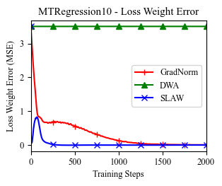
Figure 1: Loss weight error on MTRegression, or the MSE between current loss weights and ideal weights, averaged over 10 training runs. For visual clarity, the loss weight error is shown for only the first 20% of training.

4.2 Performance (NYUv2)

	Avg Acc	Stdev Acc	Seg Pixel Acc	SN Acc	Depth Acc	Step Time
Constant	$61.469\pm 0.253$	$9.542$	$\mathbf{69.510}\pm 0.164$	$48.280\pm 0.452$	$\mathbf{66.962}\pm 0.308$	$\mathbf{0.573}$
Uncertainty	$61.074\pm 0.308$	$9.602$	$\mathbf{69.277}\pm 0.321$	$47.950\pm 0.406$	$66.467\pm 0.414$	$0.577$
GradNorm	$\mathbf{62.286}\pm 0.329$	$8.612$	$69.167\pm 0.126$	$\mathbf{50.547}\pm 0.552$	$\mathbf{67.646}\pm 0.448$	$1.243$
DWA	$61.219\pm 0.297$	$9.656$	$\mathbf{69.529}\pm 0.169$	$48.071\pm 0.403$	$66.705\pm 0.336$	$0.587$
PCGrad	$61.313\pm 0.242$	$9.349$	$\mathbf{69.699}\pm 0.178$	$48.372\pm 0.233$	$66.686\pm 0.357$	$1.133$
SLAW (Ours)	$\mathbf{61.798}\pm 0.363$	$\mathbf{7.917}$	$69.133\pm 0.124$	$\mathbf{51.238}\pm 0.417$	$65.623\pm 0.670$	$0.592$

Table 2: Multi-task NYUv2 test results for semantic segmentation, surface normal estimation, and depth prediction, averaged over 10 runs with 95% confidence intervals. The result of the best performing method is bolded, as well any result whose confidence interval intersects that of the best result. GradNorm and SLAW achieve the highest average accuracy, though each training step with GradNorm takes over twice as long as any other method. SLAW exhibits the most equity across the 3 tasks.

Training Settings

NYUv2 [27] consists of 1449 RGB images which are densely labeled for semantic segmentation (13 classes), surface normal estimation, and depth prediction. The 795 training images and 654 testing images depict indoor scenes with resolution 640x480, though we downscale the images to 160x120.

Our multi-task architecture for NYUv2 is designed following [18], with some simplifications. The network consists of a feature extractor shared by all tasks, followed by task-specific output branches. The shared feature extractor is a ResNet-50 [16] pretrained on ImageNet classification [35], cut off before the final average pooling layer. Each task-specific branch has 3 3x3 Conv-BN-ReLU layers with 256 channels in the first two layers.

This unified architecture is trained by minimizing the weighted sum of task-specific losses: $w_{1}L_{1}+w_{2}L_{2}+w_{3}L_{3}$. Here $L_{1},L_{2}$, and $L_{3}$ represent the loss functions for semantic segmentation, surface normal estimation, and depth prediction respectively. $L_{1}$ is the pixel-wise mean of the cross entropy loss, $L_{2}$ is the negative pixel-wise mean of cosine similarity, and $L_{3}$ is the scale-invariant loss for depth prediction used for training in [13].

We train for 20 epochs with a batch size of 36, following the table of hyperparameters given in Appendix C. For each method, we run 10 training runs with different random seeds and report the average metric values over the 10 runs.

To evaluate all tasks on common ground, we define an accuracy metric for each task. For semantic segmentation we measure the percentage of correctly classified pixels. Performance on normal estimation is measured as the percentage of pixels for which the angle between the ground truth normal and the predicted normal is less than 11.25 degrees. Lastly, for depth prediction we define accuracy as the percentage of pixels for which the ratio between the ground truth and predicted depth is between 0.8 and 1.25. We then report the mean of task accuracies as a measure of overall performance and the standard deviation of task accuracies as a measure of inequity across tasks.

Results

Results are shown in Table 2. SLAW and GradNorm achieve the highest average accuracy across the three tasks, with a statistically significant difference between these two methods and the other baselines. In addition, the spread of accuracies across the three tasks is smallest when training with SLAW. Therefore, SLAW exhibits the best overall performance and the most equitable training of tasks.

However, the increased average performance of SLAW and GradNorm doesn’t come from an increase on every task; these two methods incur a trade-off between task performances. For example, SLAW and GradNorm are superior in surface normal estimation and depth prediction, respectively, but both methods are outperformed by the other baselines in semantic segmentation.

While GradNorm reaches the highest average accuracy, each of its training steps requires more than double the time of any other method. SLAW retains the strong performance of GradNorm while enjoying a significant boost in speed.

4.3 Efficiency (PCBA)

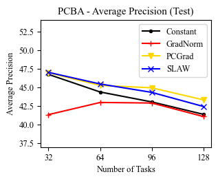
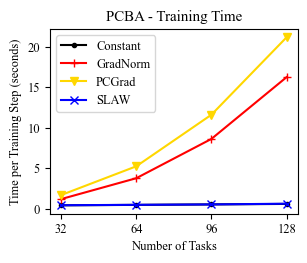
Figure 2: Average precision (AP) and time per training step vs. number of tasks on PCBA. As the number of tasks grows from 32 to 128, training time stays nearly constant for SLAW, while the train step times for GradNorm and PCGrad grow by factors of 13.1 and 12.2, respectively (right). SLAW achieves a higher AP than GradNorm and is competitive with PCGrad (left).

Training Settings

The PubChem BioAssay (PCBA) dataset [37] contains data for 128 virtual screening tasks. Virtual screening [33] is the process of predicting whether a candidate molecule will bind to a biological target in order to identify promising compounds for new drugs. The 128 tasks are binary classification of candidate molecules as either active or inactive for 128 different biological targets. In total, about 440K candidate molecules are labeled, though each molecule is labeled for an average of 78 tasks, yielding over 34 million labeled candidate/target pairs. The classes are not balanced; on average, only about 2% of input molecules will bind to a given target. We use the PCBA data hosted in the DeepChem [30] repository.

Each input molecule is featurized as a 2048-length binary vector using RDKit [20] to compute ECFP features [32] (radius 4). We use the Pyramidal architecture of [31]: a fully-connected network made of a 2-layer shared feature extractor and 1-layer task-specific output heads. The feature extractor layers have 2000 and 100 units, respectively. Our loss function is the weighted sum of the cross-entropy classification loss for each task. To account for class imbalance, we scale the loss for each class by a factor inversely proportional to the number of samples of that class.

We train on datasets with varying number of tasks and analyze each method’s computation time as a function of the number of tasks. From the 128 tasks in PCBA, we construct four multi-task datasets with 32, 64, 96, and 128 tasks. Since some molecules aren’t labeled for any of the tasks in the first three datasets, we restrict these experiments to the subset of input molecules which are labeled for at least one of the first 32 tasks, leaving about 390K input molecules. Of these remaining inputs, we use 90% for training and 10% for testing. For each dataset, we train for 100 epochs with a batch size of 40000, following the table of hyperparameters from Appendix C. Efficiency and performance are evaluated with time per training step and the mean of the Average Precision (AP) over all tasks, averaged over 5 random seeds.

Results

Results are shown in Figure 2. The training step time for GradNorm and PCGrad grows significantly with the number of tasks, since these methods compute one (at least partial) backwards pass per task for each training step. As the number of tasks grows from 32 to 128, the train step times for GradNorm and PCGrad each grow by a factor of more than 12, taking 16.2 seconds and 21.1 seconds, respectively, per training step on 128 tasks. In contrast, the train step time of SLAW is nearly identical to Constant, increasing only by a factor of 1.4 from 32 to 128 tasks. When training on the full task set, SLAW trains 24.4 times faster than GradNorm and 33.0 times faster than PCGrad.

Despite the efficiency gains, SLAW consistently achieves a larger average precision than GradNorm, and is competitive with PCGrad. Interestingly, GradNorm is outperformed by even the naive baseline Constant, but the gap between these methods shrinks as the number of tasks increases. We conclude that SLAW can be efficiently scaled to a large number of tasks without sacrificing performance.

5 Conclusion

In this paper, we introduced Scaled Loss Approximate Weighting (SLAW), an efficient and general method for multi-task optimization that requires little to no hyperparameter tuning. SLAW matches the performance of existing methods, but runs much faster by estimating the norms of the gradients of each task’s loss function instead of computing gradients directly. We provided theoretical and empirical justification for the estimation of these gradient norms, and we showed that SLAW directly estimates a solution to a special case of the optimization problem that GradNorm [5] iteratively solves. Experimental results on a collection of non-linear regression tasks, NYUv2, and virtual screening for drug discovery show that SLAW can learn to ideally balance learning between tasks, matches or exceeds the performance of existing methods, is much more efficient than existing methods, and is scalable to many tasks.

Efficiency and scalability to large collections of tasks are key qualities for MTL algorithms. Until MTL [40, 8] and the related fields of meta-learning [17] and lifelong learning [10] reach their potential, we will be trapped in the era of gathering huge labeled datasets and slowly retraining from scratch on each new task. The compute and data efficiency gains afforded by MTL may help us leave this era, but making this a reality will require improving the speed, performance, and flexibility of MTL methods.

Appendix A Proof of Theorem 1

Proof.

For a given $\mathbf{x}_{0}\in\mathbb{R}^{d}$ and $\epsilon>0$, let $\epsilon_{1}=\sqrt{\epsilon}$ and $\epsilon_{2}=\frac{\epsilon}{4K}$. Let $\delta_{1}$ be such that $|f(\mathbf{x})-f(\mathbf{x}_{0})|<\epsilon_{1}$ whenever $|\mathbf{x}-\mathbf{x}_{0}|<\delta_{1}$ and let $\delta_{2}$ be such that $\|\nabla f(\mathbf{x})-\nabla f(\mathbf{x}_{0})\|<\epsilon_{2}$ whenever $|\mathbf{x}-\mathbf{x}_{0}|<\delta_{2}$. Let $\delta=\min(\delta_{1},\delta_{2},1)$. Let $\mathbf{X}$ be a random variable which is uniformly distributed over $\{\mathbf{x}_{0}+\mathbf{d}:\|\mathbf{d}\|<\delta\}$. Then let $K_{1}=\mathbb{E}\left[\cos^{2}\theta~{}\|\mathbf{X}-\mathbf{x}_{0}\|^{2}\right]$ (where $\theta$ is the angle between $\mathbf{X}-\mathbf{x}_{0}$ and $(1,0,...,0,0)$), $K_{3}=\mathbb{E}\left[\|\mathbf{X}-\mathbf{x}_{0}\|^{2}\right]$, and $K_{2}=\epsilon_{2}^{2}K_{3}-\epsilon_{1}^{2}/2$.

Now, let $\mu=\mathbb{E}[f(\mathbf{X})]$. Then by linearity of expectation:

$$\text{Var}[f(\mathbf{X})] =\mathbb{E}[(f(\mathbf{X})-\mu)^{2}]$$ (16)

$$=\mathbb{E}[((f(\mathbf{X})-f(\mathbf{x}_{0}))-(\mu-f(\mathbf{x}_{0})))^{2}]$$ (17)

$$=\mathbb{E}[(f(\mathbf{X})-f(\mathbf{x}_{0}))^{2}]-2\mathbb{E}[(f(\mathbf{X})-f(\mathbf{x}_{0}))(\mu-f(\mathbf{x}_{0}))]+(\mu-f(\mathbf{x}_{0}))^{2}$$ (18)

$$=\mathbb{E}[(f(\mathbf{X})-f(\mathbf{x}_{0}))^{2}]-(\mu-f(\mathbf{x}_{0}))^{2},$$ (19)

We will bound $\text{Var}[f(\mathbf{\mathbf{X}})]$ by bounding each of the two terms in Equation 19 individually. Starting with $(\mu-f(\mathbf{x}_{0}))^{2}$, we know that $\mu=f(\mathbf{a})$ for some $\mathbf{a}$ with $\|\mathbf{a}-\mathbf{x}_{0}\|<\delta$ by applying the intermediate value theorem. Therefore

$$(\mu-f(\mathbf{x}_{0}))^{2}=(f(\mathbf{a})-f(\mathbf{x}_{0}))^{2}\leq\epsilon_{1}^{2}$$ (20)

where the upper bound comes from the fact that $\|\mathbf{a}-\mathbf{x}_{0}\|<\delta<\delta_{1}$. This gives the bound

$$0\leq(\mu-f(\mathbf{x}_{0}))^{2}\leq\epsilon_{1}^{2}$$ (21)

To bound $\mathbb{E}[(f(\mathbf{X})-f(\mathbf{x}_{0}))^{2}]$, the second term from Equation 19, let $\mathbf{x}\in\mathbb{R}^{d}$ with $\|\mathbf{x}-\mathbf{x}_{0}\|<\delta$, $\mathbf{u}=(\mathbf{x}-\mathbf{x_{0}})/\|\mathbf{x}-\mathbf{x_{0}}\|$. For $t\in[0,\|\mathbf{x}-\mathbf{x}_{0}\|]$, let $\mathbf{x}_{t}=\mathbf{x}_{0}+t\mathbf{u}$ and $\mathbf{d}_{t}=\nabla f(\mathbf{x}_{t})-\nabla f(\mathbf{x}_{0})$. By the fundamental theorem of calculus, we have:

$$|f(\mathbf{x})-f(\mathbf{x}_{0})| =\left|\int_{0}^{\|\mathbf{x}-\mathbf{x}_{0}\|}D_{\mathbf{u}}f(\mathbf{x}_{t})~{}dt\right|$$ (22)

$$=\left|\int_{0}^{\|\mathbf{x}-\mathbf{x}_{0}\|}\nabla f(\mathbf{x}_{t})\cdot\mathbf{u}~{}dt\right|$$ (23)

$$=\left|\int_{0}^{\|\mathbf{x}-\mathbf{x}_{0}\|}\nabla f(\mathbf{x}_{0})\cdot\mathbf{u}~{}dt+\int_{0}^{\|\mathbf{x}-\mathbf{x}_{0}\|}\mathbf{d}_{t}\cdot\mathbf{u}~{}dt\right|$$ (24)

$$=\left|\nabla f(\mathbf{x}_{0})\cdot(\mathbf{x}-\mathbf{x}_{0})+\int_{0}^{\|\mathbf{x}-\mathbf{x}_{0}\|}\mathbf{d}_{t}\cdot\mathbf{u}~{}dt\right|,$$ (25)

Applying the triangle inequality to Equation 25, we obtain:

$$|f(\mathbf{x})-f(\mathbf{x}_{0})| \leq|\nabla f(\mathbf{x}_{0})\cdot(\mathbf{x}-\mathbf{x}_{0})|+\left|\int_{0}^{\|\mathbf{x}-\mathbf{x}_{0}\|}\mathbf{d}_{t}\cdot\mathbf{u}~{}dt\right|$$ (26)

$$\leq|\nabla f(\mathbf{x}_{0})\cdot(\mathbf{x}-\mathbf{x}_{0})|+\int_{0}^{\|\mathbf{x}-\mathbf{x}_{0}\|}|\mathbf{d}_{t}\cdot\mathbf{u}|~{}dt$$ (27)

$$\leq|\nabla f(\mathbf{x}_{0})\cdot(\mathbf{x}-\mathbf{x}_{0})|+\int_{0}^{\|\mathbf{x}-\mathbf{x}_{0}\|}\|\mathbf{d}_{t}\|~{}dt$$ (28)

$$<|\nabla f(\mathbf{x}_{0})\cdot(\mathbf{x}-\mathbf{x}_{0})|+\epsilon_{2}\|\mathbf{x}-\mathbf{x}_{0}\|$$ (29)

$$=|(\|\nabla f(\mathbf{x}_{0})\|\cos\theta+\epsilon_{2})\|\mathbf{x}-\mathbf{x}_{0}\|,$$ (30)

where $\theta$ is the angle between $\nabla f(\mathbf{x}_{0})$ and $\mathbf{x}-\mathbf{x}_{0}$. We can obtain a similar lower bound by again applying the triangle inequality in a slightly different form to Equation 25:

$$|f(\mathbf{x})-f(\mathbf{x}_{0})| \geq|\nabla f(\mathbf{x}_{0})\cdot(\mathbf{x}-\mathbf{x}_{0})|-\left|\int_{0}^{\|\mathbf{x}-\mathbf{x}_{0}\|}\mathbf{d}_{t}\cdot\mathbf{u}~{}dt\right|$$ (31)

which, by an identical computation as above, leads to the lower bound:

$$|f(\mathbf{x})-f(\mathbf{x}_{0})| >|(\|\nabla f(\mathbf{x}_{0})\|\cos\theta-\epsilon_{2})\|\mathbf{x}-\mathbf{x}_{0}\|,$$ (32)

Therefore, from Equation 30, we have

$$\mathbb{E}\left[(f(\mathbf{X})-f(\mathbf{x}_{0}))^{2}\right] <\mathbb{E}\left[(\|\nabla f(\mathbf{x}_{0})\|\cos\theta-\epsilon_{2})^{2}\|\mathbf{X}-\mathbf{x}_{0}\|^{2}\right]$$ (33)

$$<\|\nabla f(\mathbf{x}_{0})\|^{2}~{}\mathbb{E}\left[\cos^{2}\theta~{}\|\mathbf{X}-\mathbf{x}_{0}\|^{2}\right]+2\epsilon_{2}\|\nabla f(\mathbf{x}_{0})\|~{}\mathbb{E}\left[\|\mathbf{X}-\mathbf{x}_{0}\|^{2}\right]+\epsilon_{2}^{2}\mathbb{E}\left[\|\mathbf{X}-\mathbf{x}_{0}\|^{2}\right]$$ (34)

Since $f$ is $K$-Lipschitz, we have $\|\nabla f(\mathbf{x}_{0})\|\leq K$. So

$$\mathbb{E}\left[(f(\mathbf{X})-f(\mathbf{x}_{0}))^{2}\right]<K_{1}\|\nabla f(\mathbf{x}_{0})\|^{2}+2\epsilon_{2}KK_{3}+\epsilon_{2}^{2}K_{3},$$ (35)

Performing the same operations with the lower bound of $|f(\mathbf{x})-f(\mathbf{x}_{0})|$ from Equation 32, we obtain:

$$\mathbb{E}\left[(f(\mathbf{X})-f(\mathbf{x}_{0}))^{2}\right]>K_{1}\|\nabla f(\mathbf{x}_{0})\|^{2}-2\epsilon_{2}KK_{3}+\epsilon_{2}^{2}K_{3},$$ (36)

We can now derive an upper bound for $\text{Var}[f(\mathbf{X})]$ by plugging Equations 21 and 35 into Equation 19:

$$\text{Var}[f(\mathbf{X})] <K_{1}\|\nabla f(\mathbf{x}_{0})\|^{2}+2\epsilon_{2}KK_{3}+\epsilon_{2}^{2}K_{3}$$ (37)

$$\text{Var}[f(\mathbf{X})]-(K_{1}\|\nabla f(\mathbf{x}_{0})\|^{2}+\epsilon_{2}^{2}K_{3}) <2\epsilon_{2}KK_{3}$$ (38)

$$\text{Var}[f(\mathbf{X})]-(K_{1}\|\nabla f(\mathbf{x}_{0})\|^{2}+\epsilon_{2}^{2}K_{3}-\epsilon_{1}^{2}/2) <2\epsilon_{2}KK_{3}+\epsilon_{1}^{2}/2,$$ (39)

Similarly, to derive a lower bound for $\text{Var}[f(\mathbf{X})]$, we plug Equations 21 and 36 into Equation 19:

$$\text{Var}[f(\mathbf{X})] >K_{1}\|\nabla f(\mathbf{x}_{0})\|^{2}-2\epsilon_{2}KK_{3}+\epsilon_{2}^{2}K_{3}-\epsilon_{1}^{2}$$ (40)

$$\text{Var}[f(\mathbf{X})]-(K_{1}\|\nabla f(\mathbf{x}_{0})\|^{2}+\epsilon_{2}^{2}K_{3}) >-2\epsilon_{2}KK_{3}-\epsilon_{1}^{2}$$ (41)

$$\text{Var}[f(\mathbf{X})]-(K_{1}\|\nabla f(\mathbf{x}_{0})\|^{2}+\epsilon_{2}^{2}K_{3}-\epsilon_{1}^{2}/2) >-2\epsilon_{2}KK_{3}-\epsilon_{1}^{2}/2,$$ (42)

Recall that $\delta<1$, so $K_{3}<1$. Finally, combining Equations 39 and 42:

$$\left|\text{Var}[f(\mathbf{X})]-(K_{1}\|\nabla f(\mathbf{x}_{0})\|^{2}+\epsilon_{2}^{2}K_{3}-\epsilon_{1}^{2}/2)\right| <2\epsilon_{2}KK_{3}+\epsilon_{1}^{2}/2$$ (43)

$$\left|\text{Var}[f(\mathbf{X})]-(K_{1}\|\nabla f(\mathbf{x}_{0})\|^{2}+\epsilon_{2}^{2}K_{3}-\epsilon_{1}^{2}/2)\right| <2\epsilon_{2}K+\epsilon_{1}^{2}/2$$ (44)

$$\left|\text{Var}[f(\mathbf{X})]-(K_{1}\|\nabla f(\mathbf{x}_{0})\|^{2}+K_{2})\right| <\epsilon/2+\epsilon/2$$ (45)

$$\left|\text{Var}[f(\mathbf{X})]-(K_{1}\|\nabla f(\mathbf{x}_{0})\|^{2}+K_{2})\right| <\epsilon$$ (46)

∎

Appendix B Empirical Validation of SLAW

We conduct an empirical validation of SLAW by checking the accuracy of SLAW’s estimate of gradient magnitudes. Specifically, for task gradient $g_{i}=\nabla L_{i}$, SLAW estimates $\|g_{i}\|$ with $s_{i}$ as defined in Equations 6, 7, and 8. However, $s_{i}$ is not an unbiased estimate of $\|g_{i}\|$. Theorem 1 only tells us that $s_{i}$ is nearly proportional to $\|g_{i}\|$. For our case, nearly proportional is good enough. The end goal of this estimation is not to estimate the magnitudes $\|g_{i}\|$ exactly, but to estimate the relative magnitudes of each $\|g_{i}\|$ as described by Equation 4. We postulate that this can be estimated with the relative magnitudes of each $s_{i}$.

To evaluate whether SLAW can accurately estimate the weights specified by Equation 4, we collect samples of SLAW’s estimation $s_{i}$ along with the true gradient norms $\|g_{i}\|$ during training on the MTRegression dataset. For each sample of $s_{i}$ and $\|g_{i}\|$, we plot the pair $(x,y)$ defined as follows:

$$x =\frac{n}{\|g_{i}\|}\bigg{/}\sum_{j=1}^{n}\frac{1}{\|g_{j}\|}$$ (47)

$$y =\frac{n}{s_{i}}\bigg{/}\sum_{j=1}^{n}\frac{1}{s_{i}}$$ (48)

Each sample is taken during a randomly chosen step of training between training step 10 and training step 1000. We cut off the sampling at training step 1000 in order to ensure that the experiment ran in a reasonable amount of time. Also, each sample is generated from a different training run, to ensure that all points on the plot are independently generated. The color and marker of each data point corresponds to the task whose gradient is being estimated by SLAW.

Figure 3 shows the result of plotting 120 such $(x,y)$ pairs. The figure shows that each $x$ provides a close approximation to the corresponding $y$. From this, we conclude that SLAW computes a valid estimation of the task gradient norms, and the loss weights learned by SLAW are close to the loss weights specified by Equation 4.

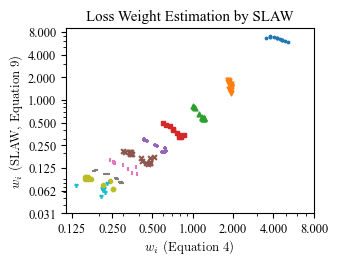
Figure 3: Empirical validation of SLAW’s estimate of the gradient norm while training on MTRegression dataset. Each data point shows the value of a loss weight $w_{i}$ as assigned by Equation 4 on a random training step (x-axis) and SLAW’s weight value as assigned by Equation 9 on the same step (y-axis). The color and marker shape of each point corresponds to the task index $i$ for which the true and estimated gradients are plotted. Each data point is generated from a different training run to ensure independence.

Appendix C Experiment Hyperparameters

All hyperparameters specific to the loss weighting method were chosen to match the values provided by the original papers.

	MTRegression	NYUv2	PCBA
Epochs	300	20	100
Batch size	304	36	40000
Learning rate	7e-4	7e-4	3e-4
Gradient clipping (max gradient norm)	0.5	0.5	0.5
Backbone architecture	FC (4 layer)	ResNet-50	Pyramidal [31]
Hidden size	100	N/A	2000, 100
Activation function	Tanh	ReLU	ReLU
Moving average coefficient (SLAW/DWA)	0.99/0.9	0.99/0.9	0.99/0.9
Loss weight LR (GradNorm)	0.025	0.025	0.025
Asymmetry (GradNorm)	0.12	1.5	0.12
Loss weight temperature (DWA)	2.0	2.0	2.0

References

- [1] Alessandro Achille, Michael Lam, Rahul Tewari, Avinash Ravichandran, Subhransu Maji, Charless C Fowlkes, Stefano Soatto, and Pietro Perona. Task2vec: Task embedding for meta-learning. In Proceedings of the IEEE/CVF International Conference on Computer Vision, pages 6430–6439, 2019.
- [2] Héctor Martínez Alonso and Barbara Plank. When is multitask learning effective? semantic sequence prediction under varying data conditions. arXiv preprint arXiv:1612.02251, 2016.
- [3] Rich Caruana. Multitask learning. Machine Learning, 28(1):41–75, 1997.
- [4] Arslan Chaudhry, Marc’Aurelio Ranzato, Marcus Rohrbach, and Mohamed Elhoseiny. Efficient lifelong learning with a-gem. arXiv preprint arXiv:1812.00420, 2018.
- [5] Zhao Chen, Vijay Badrinarayanan, Chen-Yu Lee, and Andrew Rabinovich. Gradnorm: Gradient normalization for adaptive loss balancing in deep multitask networks, 2017.
- [6] Travers Ching, Daniel S. Himmelstein, Brett K. Beaulieu-Jones, Alexandr A. Kalinin, Brian T. Do, Gregory P. Way, Enrico Ferrero, Paul-Michael Agapow, Michael Zietz, Michael M. Hoffman, Wei Xie, Gail L. Rosen, Benjamin J. Lengerich, Johnny Israeli, Jack Lanchantin, Stephen Woloszynek, Anne E. Carpenter, Avanti Shrikumar, Jinbo Xu, Evan M. Cofer, Christopher A. Lavender, Srinivas C. Turaga, Amr M. Alexandari, Zhiyong Lu, David J. Harris, Dave DeCaprio, Yanjun Qi, Anshul Kundaje, Yifan Peng, Laura K. Wiley, Marwin H. S. Segler, Simina M. Boca, S. Joshua Swamidass, Austin Huang, Anthony Gitter, and Casey S. Greene. Opportunities and obstacles for deep learning in biology and medicine. Journal of The Royal Society Interface, 15(141):20170387, 2018.
- [7] Ronan Collobert and Jason Weston. A unified architecture for natural language processing: Deep neural networks with multitask learning. In Proceedings of the 25th International Conference on Machine Learning, ICML ’08, page 160–167, New York, NY, USA, 2008. Association for Computing Machinery.
- [8] Michael Crawshaw. Multi-task learning with deep neural networks: A survey, 2020.
- [9] Jifeng Dai, Kaiming He, and Jian Sun. Instance-aware semantic segmentation via multi-task network cascades, 2015.
- [10] Matthias Delange, Rahaf Aljundi, Marc Masana, Sarah Parisot, Xu Jia, Ales Leonardis, Greg Slabaugh, and Tinne Tuytelaars. A continual learning survey: Defying forgetting in classification tasks. IEEE Transactions on Pattern Analysis and Machine Intelligence, 2021.
- [11] Long Duong, Trevor Cohn, Steven Bird, and Paul Cook. Low resource dependency parsing: Cross-lingual parameter sharing in a neural network parser. In Proceedings of the 53rd Annual Meeting of the Association for Computational Linguistics and the 7th International Joint Conference on Natural Language Processing (Volume 2: Short Papers), pages 845–850, Beijing, China, July 2015. Association for Computational Linguistics.
- [12] David Eigen and Rob Fergus. Predicting depth, surface normals and semantic labels with a common multi-scale convolutional architecture, 2015.
- [13] David Eigen, Christian Puhrsch, and Rob Fergus. Depth map prediction from a single image using a multi-scale deep network. In 28th Annual Conference on Neural Information Processing Systems 2014, NIPS 2014, pages 2366–2374. Neural information processing systems foundation, 2014.
- [14] Yuan Gao, Jiayi Ma, Mingbo Zhao, Wei Liu, and Alan L Yuille. Nddr-cnn: Layerwise feature fusing in multi-task cnns by neural discriminative dimensionality reduction. In Proceedings of the IEEE Conference on Computer Vision and Pattern Recognition, pages 3205–3214, 2019.
- [15] Michelle Guo, Albert Haque, De-An Huang, Serena Yeung, and Li Fei-Fei. Dynamic task prioritization for multitask learning. In Vittorio Ferrari, Martial Hebert, Cristian Sminchisescu, and Yair Weiss, editors, Computer Vision – ECCV 2018, pages 282–299, Cham, 2018. Springer International Publishing.
- [16] Kaiming He, Xiangyu Zhang, Shaoqing Ren, and Jian Sun. Deep residual learning for image recognition. In 2016 IEEE Conference on Computer Vision and Pattern Recognition (CVPR), pages 770–778, 2016.
- [17] Timothy M Hospedales, Antreas Antoniou, Paul Micaelli, and Amos J Storkey. Meta-learning in neural networks: A survey. IEEE Transactions on Pattern Analysis and Machine Intelligence, 2021.
- [18] Alex Kendall, Yarin Gal, and Roberto Cipolla. Multi-task learning using uncertainty to weigh losses for scene geometry and semantics, 2017.
- [19] Diederik Kingma and Jimmy Ba. Adam: A method for stochastic optimization. International Conference on Learning Representations, 12 2014.
- [20] Greg Landrum. Rdkit: Open-source cheminformatics, 2006.
- [21] Liyang Liu, Yi Li, Zhanghui Kuang, Jing-Hao Xue, Yimin Chen, Wenming Yang, Qingmin Liao, and Wayne Zhang. Towards impartial multi-task learning. In International Conference on Learning Representations, 2020.
- [22] S. Liu, E. Johns, and A. J. Davison. End-to-end multi-task learning with attention. In 2019 IEEE/CVF Conference on Computer Vision and Pattern Recognition (CVPR), pages 1871–1880, 2019.
- [23] Shengchao Liu, Yingyu Liang, and Anthony Gitter. Loss-balanced task weighting to reduce negative transfer in multi-task learning. In Proceedings of the AAAI Conference on Artificial Intelligence, volume 33, pages 9977–9978, 2019.
- [24] Yongxi Lu, Abhishek Kumar, Shuangfei Zhai, Yu Cheng, Tara Javidi, and Rogerio Feris. Fully-adaptive feature sharing in multi-task networks with applications in person attribute classification. In Proceedings of the IEEE conference on computer vision and pattern recognition, pages 5334–5343, 2017.
- [25] Riccardo Miotto, Fei Wang, Shuang Wang, Xiaoqian Jiang, and Joel T Dudley. Deep learning for healthcare: review, opportunities and challenges. Briefings in Bioinformatics, 19(6):1236–1246, 05 2017.
- [26] Ishan Misra, Abhinav Shrivastava, Abhinav Gupta, and Martial Hebert. Cross-stitch networks for multi-task learning. In Proceedings of the IEEE Conference on Computer Vision and Pattern Recognition, pages 3994–4003, 2016.
- [27] Pushmeet Kohli Nathan Silberman, Derek Hoiem and Rob Fergus. Indoor segmentation and support inference from rgbd images. In ECCV, 2012.
- [28] Emilio Parisotto, Jimmy Lei Ba, and Ruslan Salakhutdinov. Actor-mimic: Deep multitask and transfer reinforcement learning. arXiv preprint arXiv:1511.06342, 2015.
- [29] Lerrel Pinto and Abhinav Gupta. Learning to push by grasping: Using multiple tasks for effective learning. In 2017 IEEE International Conference on Robotics and Automation (ICRA), pages 2161–2168. IEEE, 2017.
- [30] Bharath Ramsundar, Peter Eastman, Patrick Walters, Vijay Pande, Karl Leswing, and Zhenqin Wu. Deep Learning for the Life Sciences. O’Reilly Media, 2019.
- [31] Bharath Ramsundar, Steven Kearnes, Patrick Riley, Dale Webster, David Konerding, and Vijay Pande. Massively multitask networks for drug discovery. arXiv preprint arXiv:1502.02072, 2015.
- [32] David Rogers and Mathew Hahn. Extended-connectivity fingerprints. Journal of Chemical Information and Modeling, 50(5):742–754, April 2010.
- [33] Judith M. Rollinger, Hermann Stuppner, and Thierry Langer. Virtual screening for the discovery of bioactive natural products, pages 211–249. Birkhäuser Basel, Basel, 2008.
- [34] Sebastian Ruder, Joachim Bingel, Isabelle Augenstein, and Anders Søgaard. Latent multi-task architecture learning. In Proceedings of the AAAI Conference on Artificial Intelligence, volume 33, pages 4822–4829, 2019.
- [35] Olga Russakovsky, Jia Deng, Hao Su, Jonathan Krause, Sanjeev Satheesh, Sean Ma, Zhiheng Huang, Andrej Karpathy, Aditya Khosla, Michael Bernstein, et al. Imagenet large scale visual recognition challenge. International journal of computer vision, 115(3):211–252, 2015.
- [36] Trevor Standley, Amir R Zamir, Dawn Chen, Leonidas Guibas, Jitendra Malik, and Silvio Savarese. Which tasks should be learned together in multi-task learning? arXiv preprint arXiv:1905.07553, 2019.
- [37] Yanli Wang, Stephen H. Bryant, Tiejun Cheng, Jiyao Wang, Asta Gindulyte, Benjamin A. Shoemaker, Paul A. Thiessen, Siqian He, and Jian Zhang. PubChem BioAssay: 2017 update. Nucleic Acids Research, 45(D1):D955–D963, 11 2016.
- [38] Tianhe Yu, Saurabh Kumar, Abhishek Gupta, Sergey Levine, Karol Hausman, and Chelsea Finn. Gradient surgery for multi-task learning. Advances in Neural Information Processing Systems, 33, 2020.
- [39] Amir R Zamir, Alexander Sax, William Shen, Leonidas J Guibas, Jitendra Malik, and Silvio Savarese. Taskonomy: Disentangling task transfer learning. In Proceedings of the IEEE conference on computer vision and pattern recognition, pages 3712–3722, 2018.
- [40] Yu Zhang and Qiang Yang. A survey on multi-task learning. arXiv preprint arXiv:1707.08114, 2017.
- [41] Zhanpeng Zhang, Ping Luo, Chen Change Loy, and Xiaoou Tang. Facial landmark detection by deep multi-task learning. In David Fleet, Tomas Pajdla, Bernt Schiele, and Tinne Tuytelaars, editors, Computer Vision – ECCV 2014, pages 94–108, Cham, 2014. Springer International Publishing.
- [42] Feng Zheng, Cheng Deng, Xing Sun, Xinyang Jiang, Xiaowei Guo, Zongqiao Yu, Feiyue Huang, and Rongrong Ji. Pyramidal person re-identification via multi-loss dynamic training, 2018.