Growth of Mahler measure and algebraic entropy of dynamics with the Laurent property
Abstract
We consider the growth rate of the Mahler measure in discrete dynamical systems with the Laurent property, and in cluster algebras, and compare this with other measures of growth. In particular, we formulate the conjecture that the growth rate of the logarithmic Mahler measure coincides with the algebraic entropy, which is defined in terms of degree growth. Evidence for this conjecture is provided by exact and numerical calculations of the Mahler measure for a family of Laurent polynomials generated by rank 2 cluster algebras, for a recurrence of third order related to the Markoff numbers, and for the Somos-4 recurrence. Also, for the sequence of Laurent polynomials associated with the Kronecker quiver (the cluster algebra of affine type we prove a precise formula for the leading order asymptotics of the logarithmic Mahler measure, which grows linearly.
1 Introduction, definitions and main conjecture
Given , a non-zero Laurent polynomial in variables with complex coefficients, its logarithmic Mahler measure is defined to be
| (1.1) |
obtained by integrating over all points on the -torus with respect to the Haar measure
| (1.2) |
for with local coordinates , which can be considered as the restriction to the real torus of the log-canonical meromorphic -form
| (1.3) |
on (or ), with . The name Mahler measure is also given to the quantity , but henceforth we will use the name without qualification to refer to the logarithmic version. For a polynomial in one variable of degree , with leading coefficient and roots , , the Mahler measure is found explicitly by Jensen’s formula to be
| (1.4) |
(here ), and while the existence of the -variable integral in (1.1) is not immediately obvious, it is guaranteed by a result of Lawton [43], which shows that this reduces to the case of one variable, in the sense that
| (1.5) |
In particular, this implies that for Laurent polynomials with integer coefficients. There are many interesting arithmetical questions concerning Mahler measure, like Lehmer’s problem about the smallest non-zero value of for , as well as the fact that explicit evaluations of for specific multivariable polynomials can be expressed in terms of -functions of zeta functions, or volumes of hyperbolic polyhedra [5, 11, 41]. The first such example in two variables is due to Smyth [57], who obtained the formula
| (1.6) |
in terms of the -function for the Dirichlet character .
Cluster algebras, introduced in [14], are a class of commutative algebras which, rather than being specified a priori, have distinguished sets of generators called clusters, which are produced recursively from an initial -tuple of generators by a process called mutation. One of the basic features of cluster algebras is the Laurent property: the elements in each cluster are Laurent polynomials in the initial generators, with integer coefficients. In fact, Zelevinsky once gave the following informal definition [62]: “A cluster algebra is a machine for generating non-trivial Laurent polynomials.” More precisely, a coefficient-free cluster algebra of rank is generated by starting from a seed consisting of an initial cluster of variables and a matrix that is skew-symmetrizable, in the sense that there exists a diagonal matrix of positive integers such that is skew-symmetric. Then for each integer there is a mutation , an involution which produces a new seed , where with
| (1.7) |
and with
| (1.8) |
Now for an arbitrary composition of mutations of any length , the Laurent property says that every element of the cluster belongs to , and the cluster algebra is defined to be the -algebra generated by all cluster variables in all clusters, that is . The cluster algebra is determined by the seed up to mutation equivalence, i.e. is isomorphic to for , where the equivalence relation means that for some composition of mutations .
For discrete dynamical systems defined by iteration of a rational map in dimension , there are various notions of entropy that are used to measure the growth of complexity of the iterates. Letting denote the maximum of the degrees of the rational functions defining the components of , the algebraic entropy was defined in [4] as follows.
Definition 1.1.
The algebraic entropy of a rational map is given by
| (1.9) |
Note that the existence of the above limit is guaranteed by the subadditive property of the log degrees and Fekete’s lemma [12]. This measure of growth was first used extensively to study certain birational transformations arising in statistical mechanics (see [1, 3] and references therein). For birational maps it is possible to perform blowups at singular points and reduce the computation of to a calculation in terms of the induced linear action of the pullback on the cohomology of the resulting enlarged space [10, 58], but in dimension the problem is more difficult, because where the map has singularities it is not always possible to remove exceptional hypersurfaces from the dynamical system by blowups. In general, numerical computation of the algebraic entropy of is extremely computationally intensive, because it requires exact calculation of the iterates of , and generically grows exponentially with .
Due to the fact that matrix mutations (1.7) change the exponents that appear in (1.8), and because there are possible mutations that can be applied to any cluster, generically a seed in a cluster algebra defines a set of evolutions on an -regular tree rather than a single dynamical system (apart from the so-called bipartite belt when ) [14]; nevertheless, one can define a corresponding notion of algebraic entropy, analogous to (1.9), via
| (1.10) |
where is the largest total degree of the elements in the cluster , considered as rational functions of the variables in the initial cluster . This definition only depends on the mutation equivalence class of the seed defining , as it should, because the algebraic entropy is invariant under birational transformations [4].
Inspired by Vojta’s dictionary between Nevanlinna theory and Diophantine approximation, Halburd proposed that when a rational map is defined over (or a number field), instead of degree growth it is easier (at least experimentally) to measure the growth of the logarithmic height along an orbit with specific numerical values for the initial data , where, for , , with the height being the maximum modulus of the numerators and denominators of the components of (written as fractions in lowest terms, with the convention that the number 0 has height 1). The fact that growth of (naive) height is a useful measure of complexity was already noted for birational transformations appearing in the context of statistical mechanics [1], and the additional observations made by Halburd suggest that the following definition is worthwhile.
Definition 1.2.
For a rational map (1.20), the Diophantine entropy of a particular non-singular orbit is defined by
| (1.11) |
while the Diophantine entropy of the map is taken to be
where the supremum is taken over all non-singular orbits .
In the latter definition, where it is possible the supremum can be taken over all orbits of an extension of to a regular morphism on an enlarged phase space (with the expectation being that the value of should be the same for “almost all” orbits , in an appropriate sense). Except in the case of very simple maps, an exact determination of the Diophantine entropy is usually at least as difficult as finding the algebraic entropy , but it can sometimes be computed explicitly for special families of orbits [31], and a numerical calculation of rational values of iterates along several orbits is much less computationally intensive than computing the corresponding sequence of rational functions and obtaining their degrees. Empirical evidence suggests that the algebraic entropy and the Diophantine entropy should coincide, so that , but we do not know how to prove this except for some particular maps (cases where is an integrable map in the Liouville sense [6, 46, 59], when both entropies are zero, are often the most tractable ones). Furthermore, if the dimension is large then even the exact arithmetic required to compute numerically becomes difficult.
The purpose of this article is to propose that, for discrete dynamical systems that generate Laurent polynomials, and for cluster algebras in particular, the growth of Mahler measure provides another natural notion of entropy, which in many cases coincides with the algebraic entropy and the Diophantine entropy, but is much easier to compute numerically. Before proceeding to formulate precise definitions and conjectures, we will give some motivation for why restricting to dynamics with the Laurent property need not be unnecessarily restrictive.
There are many examples of recurrences, birational maps or difference equations with the Laurent property. Some of the first known examples, discussed in [21], were recurrence relations of the form
| (1.12) |
for certain polynomials . Notable examples include a recurrence attributed to Dana Scott, that is
| (1.13) |
which produces sequences of Markoff triples: Markoff’s equation
| (1.14) |
arises in Diophantine approximation theory [8], and starting from any triple of positive integers satisfying this equation, each subsequent set of three adjacent terms generated by (1.13 is a solution, e.g. taking initial data produces the sequence
| (1.15) |
(A064098 in [50]), yielding further Markoff triples , , , etc. Another famous example is the Somos-4 recurrence
| (1.16) |
which generates the integer sequence
| (1.17) |
(A006720 in [50]) from the initial data ; for the connection with sequences of points on elliptic curves, see [29]. In tandem with the development of cluster algebras, an approach to proving the Laurent property for recurrences of the form (1.12) via the so-called Caterpillar Lemma was presented in [15], and it was subsequently shown that a large class of examples with being a sum of two monomials can be constructed systematically from cluster algebra exchange relations (1.8) defined by exchange matrices with a suitable periodicity property under sequences of mutations [19] (generalized in [49]), while examples with more than two monomials on the right-hand side arise in the broader setting of LP algebras [42]. Recurrences with the Laurent property, including those of Somos type like (1.16), also occur naturally in the theory of integrable systems, in the form of bilinear discrete Hirota equations for tau functions of lattice equations and their reductions to integrable maps/discrete Painlevé equations [18, 20, 35, 36, 38, 40, 47, 51].
However, as pointed out in [33], there is a very close connection between the Laurent property and the notion of singularity confinement, which can be combined with algebraic entropy as a tool to detect integrability (see [48] and references), and in this context one finds more general forms of discrete systems with the Laurent property which do not seem to arise from iteration of exchange relations in a cluster algebra or LP algebra. As described in [25], given a birational map with confined singularities, which need not have the Laurent property, we conjecture that it is always possible to construct its “Laurentification”, that is, a lift to a map in higher dimensions that does have the Laurent property. This conjecture is very natural in the context of discrete integrable systems, where one usually starts from a symplectic map, or a lattice equation that preserves a Poisson bracket [38], and then the existence of appropriate tau functions implies that this lifts to a system of discrete Hirota equations [60], for which the Laurent property is known to hold [15]. Beyond the setting of integrability, Hietarinta and Viallet’s example
| (1.18) |
is a symplectic map of standard type in the plane, with a parameter , that has confined singularities but displays chaotic orbits and positive entropy [28, 58]; the singularity pattern suggests lifting it to 5 dimensions via , and this provides a Laurentification of (1.18) because satisfies
| (1.19) |
with for all [32]. For other analogues of tau functions and the Laurent property for nonintegrable systems outside the setting of cluster algebras, including multidimensional generalizations of (1.18), see [39] and references.
We now formulate the main definition of entropy that we would like to consider, for the case of maps in dimension with the Laurent property, of the form
| (1.20) |
where the Laurent property means that for all , each of the components of is a Laurent polynomial in the variables appearing in the initial data with integer coefficients. Usually we are interested in birational maps, so this means , in which case can be regarded as an automorphism of the field of fractions , but it is also possible to consider non-invertible and restrict to . Then we will use to denote the maximum of the Mahler measures of the components of .
Definition 1.3.
Remark 1.4.
All of the examples considered below are of recurrence form,
with defined by a relation of the form (1.12), so that it is sufficient to take
| (1.22) |
which turns out to coincide with the preceding definition in this case.
It is also natural to consider the growth of Mahler measure for a cluster algebra defined by an initial seed , by evaluating the Mahler measure for each cluster variable belonging to a cluster obtained by a composition of mutations, and taking the limit . In this context, we let denote the maximum of the Mahler measures of the elements of the cluster .
Definition 1.5.
For a cluster algebra , the Mahler entropy is
| (1.23) |
assuming that the limit exists.
Remark 1.6.
For cluster algebras with coefficients, given by additional frozen variables that do not mutate, or for maps such as (1.19) with parameters, one can either fix specific (integer) values for these coefficients before evaluating the Mahler measure, or integrate over an additional torus for each extra parameter that appears, e.g. perform an extra integration to evaluate for the case of (1.19).
Aside from the issue of existence, it is not obvious that the above definition is independent of the choice of seed, up to mutation equivalence. However, if the Mahler entropy coincides with the algebraic entropy, then this is clearly the case.
Conjecture 1.7.
Remark 1.8.
The assumptions on mean that it is a composition of finitely many mutations in a cluster algebra, possibly also composed with a permutation of the coordinates; such maps were referred to as cluster maps in [18]. (Several examples will be given below, but see [18, 19, 49] for many more.) The above conjecture is certainly false without imposing any restriction on the class of maps with the Laurent property, as can be seen by considering the case of monomial maps, which are closely related to toral endomorphisms (or automorphisms, if we restrict to birational ). Any Laurent monomial has , hence for all monomial maps, but generic monomial maps have algebraic entropy [27].
Henceforth we will mainly be concerned with studying examples that provide evidence for the preceding conjecture. There are various reasons why it seems particularly fruitful to focus on the Mahler entropy for cluster algebras or maps generated by compositions of cluster mutations. Firstly, the meromorphic -form (1.3) is invariant under cluster mutations (1.8) up to a sign, that is , which might allow for some simplification in explicitly evaluating the Mahler measure of cluster variables. Secondly, it is already interesting to consider Mahler measure in the case of the simplest non-trivial cluster algebra, namely the cluster algebra of finite Dynkin type , obtained from the Lyness recurrence
| (1.24) |
which produces the 5-cycle of cluster variables
| (1.25) |
with the sequence repeating with period 5 thereafter. In this case, we clearly have , and from Jensen’s formula it is easy to see that , so the only non-zero Mahler measure is which is given by Smyth’s formula (1.6). (In the latter example it is clear that because the algebra is of finite type.) Thirdly, other examples of Mahler measures for cluster variables have explicit formulae in terms of the classical dilogarithm , or the Bloch-Wigner dilogarithm , evaluated at algebraic arguments (see the next section), while the dilogarithm is ubiquitous in the theory of cluster algebras, appearing in the generating functions that produce (part of) mutations as canonical transformations preserving an associated presymplectic structure, and in terms of the functional identities satisfied by or [13, 22, 35, 49]; in particular, the elements of the 5-cycle (1.25), related to the associahedron [16], correspond to the arguments in the five-term relation for [61].
Before proceeding to study other concrete examples in the rest of the paper, we present a simple result that connects the Mahler entropy with the Diophantine entropy and the algebraic entropy, but is based on the non-trivial fact of positivity for cluster variables: they are Laurent polynomials with positive coefficients, as was proved for the case of skew-symmetric in [45], and for the general case of skew-symmetrizable in [23].
Proposition 1.9.
Suppose that is a cluster map of recurrence type. Let denote the -tuple consisting of 1s, and let denote the Diophantine entropy of the orbit of with initial data . Then (assuming it exists) the Mahler entropy of satisfies
| (1.26) |
Suppose further that , for some real and , so that Conjecture 1.7 holds with . Then also.
-
Proof:
For any , the standard bounds
hold, where denotes the length of (the sum of the absolute values of the coefficients of ) and denotes the sum of the degrees of taken in each variable separately. Now suppose that is a positive Laurent polynomial generated by a cluster map of recurrence type. This means that has a canonical expression of the form
(1.27) where the polynomial is not divisible by any for , and the monomial is defined by the integer -tuple (d-vector), which consists entirely of positive integers for large enough; see [17] or [18] for further details. In terms of the total degree of as a rational function of this also means that, for sufficiently large , , and clearly . Also, by positivity we have , so substituting into the bounds above and taking logs yields
From the upper bound on , taking logs and dividing by immediately gives (1.26) in the limit . On the other hand, if and have the given asymptotic behaviour, then substituting this into the same bounds, taking logs and dividing by gives
where , and hence in the limit . ∎
Remark 1.10.
With a slightly more detailed analysis, the analogue of Proposition 1.9 should also hold for an arbitrary cluster map given (up to a permutation) by a composition of mutations, and for the corresponding entropies for any cluster algebra , but a complete proof requires keeping track of the growth of the different components within each cluster.
At this stage it is worth pointing out the numerical advantages of working with the Mahler entropy rather than using exact arithmetic to compute growth of degrees or heights of rational numbers. We will describe this for a general map with the Laurent property, but the same considerations apply to computations with cluster variables, with minor modifications. The main idea is to write an approximation to the Mahler measure of the components of the th iterate in terms of a Riemann sum, that is
| (1.28) |
where the points for belonging to some index set are equidistributed on in the limit . There are various equidistribution results in the literature which are relevant to numerical approximation of Mahler measure, in particular the work on torsion points in [2], which here corresponds to the obvious choice of a regular lattice of points on the flat torus i.e. choosing the components of to be th roots of unity, so that for , with , or the results on Gaussian periods in [24]; for a different approach, based on the doubling map, see [52]. Another convenient method, which reduces the likelihood of hitting a divergent logarithm when a point on the zero locus is chosen, is to use a Monte Carlo method, generating the points with a (pseudo)random number generator with a uniform distribution on the torus (in some sense, the doubling map used in [52] can be regarded as a pseudorandom number generator). However, regardless of what method is used to select equidistributed points , here the main point is that one can regard each choice of point as initial data for , and then one computes its orbit up to some desired , and for each adds the contribution of the th component to the sum (1.28). Thus one obtains an approximation to the Mahler measures of each Laurent polynomial appearing in the first iterates of the orbit, then takes the component with largest Mahler measure in each iterate, and all of the computations are done very rapidly with floating point arithmetic. This is in contrast to the exact arithmetic with rational functions, or with rational numbers, that is required for numerical computation of the algebraic entropy , or the Diophantine entropy , respectively.
2 Families of Laurent polynomials in rank 2
In this section we consider a family of Laurent polynomials indexed by two positive integers , generated by recurrence relations of second order, of the form
| (2.1) |
where is specified by
| (2.2) |
All recurrences of the form (2.1) preserve the log-canonical symplectic form
| (2.3) |
proportional to (1.3) when , and there are more general choices of that give the Laurent property for the map ; in particular, it was observed by Speyer that if is reciprocal, in the sense that , then (2.1) has the Laurent property, but there are other possible choices of that work (see [33, 34] for a complete classification). Here we restrict to the reciprocal polynomials (2.2) for , because they are precisely what arises from rank 2 cluster algebras defined by the skew-symmetric exchange matrices
by composing the mutation with the permutation , so that . The periodicity property and the fact that is conjugate to implies that generates all of the cluster variables, in the form of the sequence with , and the reversibility of the recurrence (2.1) implies that for all . As a consequence, we have (evidence of existence will be provided below).
Similarly, the algebraic entropy for the cluster algebra is the same as the algebraic entropy of the map , being given by
| (2.4) |
The case is the cluster algebra of finite type , generated by the cluster variables (1.25), while for the sequence of polynomials is given explicitly by the formula
| (2.5) |
obtained in [7]; there is another formula for these polynomials in terms of Chebyshev polynomials [55], and below we will employ yet another closed-form expression for all . It is clear from (2.5) that the degrees grow linearly with , hence for . There is an explicit combinatorial formula for the Laurent polynomials in terms of lattice paths [44], valid for any , but for the degree growth is exponential in , and it appears unlikely that there is any expression for the coefficients as simple as (2.5). The entropy value in (2.4) for can be derived directly from the combinatorial formula, or by writing the polynomials in the form (1.27) and using the fact that the degree vector (d-vector) of the denominator monomial in a cluster algebra satisfies the tropical version of the exchange relation, so for the recurrence (2.1) with given by (2.2) we have
| (2.6) |
satisfied componentwise, with the initial values , . For , both components of are non-negative, so they both satisfy the same scalar linear recurrence , hence for some , , and this fixes the same order of growth for the numerator of , leading to the stated value of the entropy (see e.g. [17, 18, 20] for more details on tropical dynamics and degree growth).
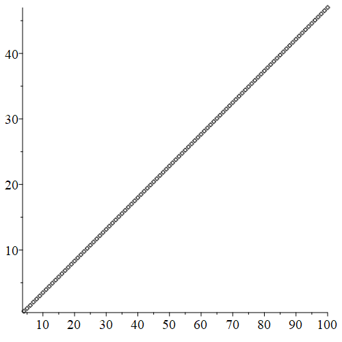
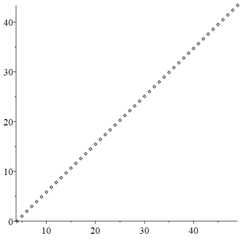
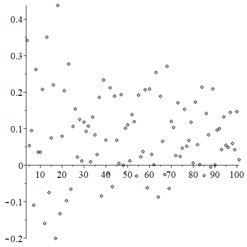
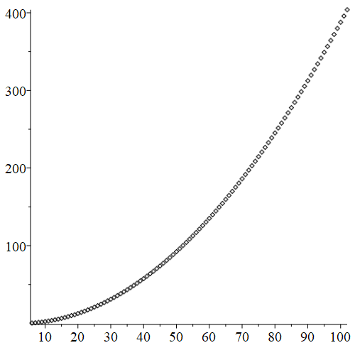
Immediate evidence for Conjecture 1.7 can be seen in Figures 1 and 2, which were obtained by computing the approximation , using (1.28) with a Monte Carlo method, picking points uniformly distributed on with a pseudorandom number generator in MAPLE; this took about one minute to produce each plot on a small laptop. For the case , the growth of appears to be linear in , as is the degree growth of the polynomials (2.5); below we will give a proof of the linear growth of Mahler measure for this case, but for now we just record the numerical estimate
| (2.7) |
for the slope in Fig.1, which should be compared with the exact value (2.17) obtained below. For the plots show exponential growth of Mahler measure, and because the growth is so rapid there is a restriction on the size of that can be calculated before MAPLE gives a floating point error; in those cases we have plotted against , up to the values , respectively. For we find the estimate for the slope, which should be compared with the value for the algebraic entropy in this case. Similarly, for we have , which is extremely close to the algebraic entropy , and for we find , which agrees with the value of to 9 d.p.
We now consider exact evaluation of these Mahler measures. The first two are clearly trivial: . More interesting to consider are the Laurent polynomials
| (2.8) |
where (for any ) the latter expression for is written most compactly with a sum over powers of , making it clear that it is an element of . Then it is easy to see from Jensen’s formula that . The next two cases will require the integral evaluation
| (2.9) |
which is used extensively in [41], where in terms of the classical dilogarithm for [61]. We will also need the Chebyshev polynomials of the first kind, defined by .
Theorem 2.1.
For each positive integer , the Mahler measure of the Laurent polynomial given in (2.8) is
| (2.10) |
which equals times the value (1.6) found by Smyth, while for the Mahler measure of is
| (2.11) |
where are the solutions of on , or equivalently are given by , with being a root of the polynomial
| (2.12) |
on the interval .
-
Proof:
First note that taking Mahler measures of both sides of (2.1) with given by (2.2) yields the recursion
(2.13) so since this gives , as powers of in the denominator make no contribution; this can also be seen directly from the formula in (2.8). Thus, by applying Jensen’s formula to carry out the integration over , we find
where we substituted and included an extra factor of coming from the fact that winds around the torus times. Then rewriting the integrand as for , this becomes
by (2.9), which equals the required answer (2.10) from the fact that is an odd function of , and for this coincides with the value (1.6), approximately . Similarly, for it is convenient to use (2.13) and to obtain
In the latter expression, we can replace without changing the Mahler measure, and then substitute as before (noting the factor of that drops out from the winding number), to find
As a polynomial in , the argument of on the right-hand side above is of degree , with roots for , so Jensen’s formula produces a sum of integrals over suitable values of , but each of these integrals transforms to the case by multiplying by a suitable power of , giving copies of the same integral, and changing variables to in this integral yields
We have already seen that this vanishes when . The value of this integral for is given by evaluating the Bloch-Wigner dilogarithm at certain corresponding to the boundary points where on the torus, given by algebraic values of modulus one that are roots of the equation , which can be converted into a polynomial in . However, for computational purposes it is more effective to set , and note that is equivalent to with , and by symmetry it is sufficient to consider the interval , where the modulus sign on the right-hand side can be removed. There are clearly solutions which we order as , and on the subintervals , ,…, up to for even, or for odd. For finding the endpoints it is convenient to rewrite the equation as , expressed in the form (2.12) with Chebyshev polynomials (note that this is a polynomial of degree because ), and then find for , . Thus, setting , and for even, we arrive at
and then writing the integrand as and applying (2.9) to each of the latter terms separately, the result (2.11) follows. ∎
In the rest of this section, we focus on the case , which is very special compared with : the dynamics of the map defined by is integrable, since there is a conserved quantity
| (2.14) |
whose level sets are conics, and also linearizable, in the sense that the iterates satisfy the linear relation
| (2.15) |
on each level set. (For many more examples of cluster variables satisfying linear relations, see [18, 19, 20, 32, 53] and references.) This means that the general solution can be parametrized explicitly as
| (2.16) |
(for ) where the parameters are related to the initial values by the same formula for and the conserved quantity is given in terms of alone by . A short calculation shows that the symplectic form is rewritten in terms of as , so in the case of real dynamics, when and there are compact Liouville tori these are the action-angle coordinates, while in the non-compact case one can introduce suitable factors of and rewrite (2.16) in terms of hyperbolic functions. (For the solution of (2.15) depends linearly on .)
Theorem 2.2.
-
Proof:
Substituting the formula (2.16) into the integral for the Mahler measure gives
where are the roots of the characteristic quadratic for the linear recurrence (2.15), and so each is given by for one of the choices of square roots. Hence we have , and the result follows. It appears that the numerical evaluation of the integral in (2.17) converges much faster with a regular grid of points on (corresponding to taking to be th roots of unity) than with the Monte Carlo method, and we have checked the value of up to 6 d.p. by taking successively . ∎

3 Recurrence for Markoff numbers
Given the exchange matrix
| (3.1) |
the mutation defines an involution on the cubic surface defined by fixing
which is associated with the moduli space of once-punctured 2-tori [9], and corresponds to Markoff’s equation (1.14) when . The same is true for the mutations , and by including the cyclic permutation , we find that , where corresponds to a single iteration of (1.13), and corresponds to two iterations. The exchange matrix (3.1) is cluster mutation-periodic with period 2, in the terminology of [19], since . In general, period 2 matrices lead to a coupling between two different relations, depending on the parity of , but in this case , so the exponents on the right-hand side are the same in both mutations, and there is just a single recurrence.
It is shown in [37] that for (1.13), and an analogous calculation with the sequence (1.15) shows that takes the same value [31]. As is well known [8], certain combinations of involutions of the Markoff surface generate solutions to Pell equations, corresponding to linear dynamics and subexponential degree growth, and it turns out that (up to symmetry) the composition of a mutation together with a permutation in corresponds to the maximum possible growth rate that can be produced by mutations alone, so also. To investigate the growth of Mahler measure, we introduce the monomials , associated with the integer basis , for , leading to the two-dimensional map defined by
| (3.2) |
which is anti-symplectic with respect to the log-canonical 2-form
| (3.3) |
Then for we can make a change of variables to rewrite (1.3) as , and from (3.2) we can recursively calculate
| (3.4) |
where the last term above reduces to an integral over the 2-torus, namely
| (3.5) |
Note that the sequence of are not all Laurent polynomials in , but rational functions in general, because (3.2) does not have the Laurent property, so in general is a difference of Mahler measures of polynomials in these two variables.
To see how this works, note that we have the trivial integrals and clearly . Then for , it follows from (3.4), (3.2) and (3.5) that by Jensen’s formula. Thus the first non-zero value turns out to be the case of , with
Then, by Jensen again, this gives an integral evaluation equal to twice (1.6), namely
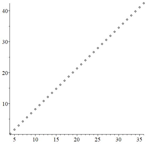
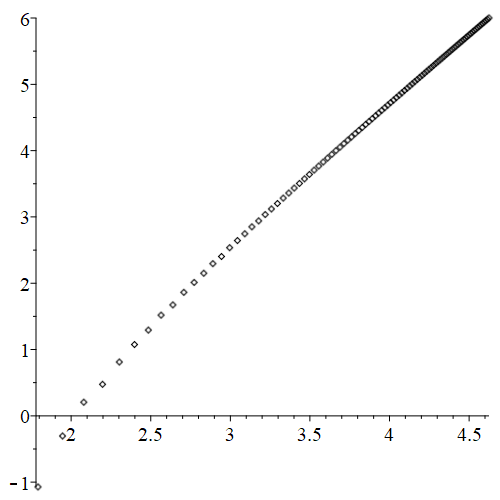
For subsequent terms in the sequence of Mahler measures given by (3.5), we have done a numerical evaluation using (1.28) with a Monte Carlo method, selecting pseudorandom points as before, iterating the map (3.2) for each of these choices of initial data to calculate an approximation to , and then applied (3.4), which allowed us to calculate as far as before getting a floating point error in MAPLE; the results are plotted in Fig.3. The approximate slope is , differing from the value of only in the 9th decimal place.
4 Somos-4 recurrence
Starting from the exchange matrix
| (4.1) |
the Somos-4 recurrence (1.16) is given by the composition , and this is an example of cluster mutation-periodicity with period 1 [19]. The d-vectors in this case grow quadratically with [18], as do the heights of the integers in (1.17) (this is related to the fact that each iteration of the map corresponds to a addition of the same point on an elliptic curve [29]), so this is an example with . Given a seed defined by (4.1), other sequences of mutations produce cluster variables with exponential degree growth, so in this case the algebraic entropy of the map does not equal .
For an efficient computation of the Mahler measures, we introduce the coordinates
| (4.2) |
which satisfy a well-known map of QRT type [54], that is
| (4.3) |
with the invariant symplectic form , and again we can rewrite (1.3), in this case with , as a log-canonical form, namely , which restricts to the 4-torus in terms of the new coordinates . Thus from (4.2) we obtain the recursion
| (4.4) |
Then just as in the Markoff case, we have a sequence of rational functions , and the problem of evaluating the Mahler measures of the 4-variable Laurent polynomials with is reduced to evaluating integrals of the form (3.5) over and applying a recursion, in this case the relation (4.4).
Now the trivial initial values are and , while for Jensen’s formula gives by (4.4), where . Thus is the first interesting case, for which (4.4) implies that the Mahler measure is
hence , the same as the value in Smyth’s result (1.6).
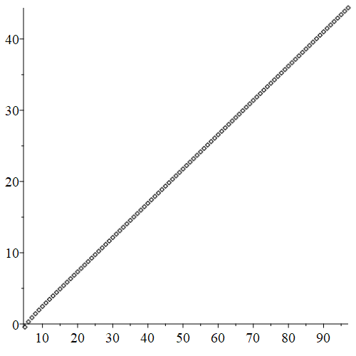
Upon doing a numerical calculation of the sequence , defined as integrals over , we observe that these values seem to oscillate quite erratically, but the corresponding sequence of approximations to the Mahler measures , obtained from the recursion (4.4), does indeed seem to trace out a parabola when plotted against , suggesting that
| (4.5) |
which would imply that indeed in this case. This quadratic growth is consistent with the growth of logarithmic heights under iterated translation by a point on an elliptic curve [56], and with the growth of degrees for maps of surfaces with an invariant elliptic fibration [10]. In Fig.4 we have also done a log-log plot, which asymptotically looks like a line with slope roughly , so very close to 2, as expected, and we have estimated the value of by calculating the differences , which suggests that .
To give more support to the conjectured asymptotic formula (4.5), we can refer to the analytic solution to the initial value problem for the Somos-4 recurrence, as presented in [29]. To be precise, the general analytic solution of (1.16) is given by
| (4.6) |
where and is the Weierstrass sigma function for an associated cubic curve . In the formula (4.6), the invariants of the associated curve and the parameters appearing in the argument of depend only on the pair of initial values for the map (4.3). This implies that the Mahler measure in this case is given to leading order by an integral over the 2-torus, namely
| (4.7) |
where and are determined by elliptic integrals, and the invariants are rational functions of . However, as it stands, the expression (4.7) does not immediately yield the result (4.5), because the term contains some hidden growth, which is best seen by rewriting this expression in terms of a Jacobi theta function (cf. the asymptotic calculation for numerical growth of Somos-5 sequences in [30]).
5 Concluding remarks
It appears that the Mahler entropy gives a useful numerical tool for measuring growth in cluster algebras and dynamical systems with the Laurent property, but so far in rank 2 we have only been able to determine it precisely for the simplest examples defined by (2.2) with . The numerical results for suggest that
but it is not clear that this follows immediately from the exact relation (2.13). If it should turn out that, to leading order, the sequence of Mahler measures satisfies a tropical version of the original dynamical system, then this could provide a key to relating it to the dynamics of d-vectors and degree growth, possibly leading to a proof of Conjecture 1.7.
A next step in a more interesting case would be to use the analytic formula in [29], expressing the solution of Somos-4 in terms of the Weierstrass sigma function, to give a proof of the conjectured asymptotics (4.5), by deriving an exact integral formula for the constant . So far we have merely indicated a possible way to go about this, using the expression (4.7), and we propose to leave the detailed analysis for future work.
It is interesting that all of the Mahler measures of cluster variables that we have been able to evaluate explicitly so far are written in terms of the Bloch-Wigner dilogarithm with algebraic arguments, similar to the examples in [41], which are related to volumes of hyperbolic polytopes. Given the connections between cluster algebras and Teichmüller theory, it is tempting to suggest that there should be a deeper explanation for this phenomenon.
Acknowledgments: This research was supported by Fellowship EP/M004333/1 from the Engineering & Physical Sciences Research Council, UK, and grant IEC\R3\193024 from the Royal Society. On behalf of all authors, the corresponding author states that there is no conflict of interest.
References
- [1] N. Abarenkova, J.-C. Anglès d’Auriac, S. Boukraa, S. Hassani, and J.-M. Maillard, Rational dynamical zeta functions for birational transformations, Phys. A 264 (1999) 264–293.
- [2] M. Baker, S. Ih and R. Rumely, A finiteness property of torsion points, Algebra Number Theory 2 (2008) 217–248.
- [3] E. Bedford and K.-H. Kim, Degree growth of matrix inversion: birational maps of symmetric, cyclic matrices, Disc. Contin. Dyn. Syst. 21 (2008) 977–1013.
- [4] M. Bellon and C.M. Viallet, Algebraic entropy, Comm. Math. Phys. 204 (1999) 425–437.
- [5] D.W. Boyd, Mahler’s measure and special values of -functions, Exp. Math. 7 (1998) 37–82.
- [6] M. Bruschi, O. Ragnisco, P.M. Santini and T. Gui-Zhang, Integrable symplectic maps, Phys. D 49 (1991) 273–294.
- [7] P. Caldero and A. V. Zelevinsky, Laurent expansions in cluster algebras via quiver representations, Mosc. Math. J. 6 (2006) 411–429.
- [8] J. W. S. Cassels, An introduction to diophantine approximation, Cambridge University Press, New York, 1957.
- [9] H. Cohn, An approach to Markoff’s minimal forms through modular functions, Ann. Math. 61 (1955) 1–12.
- [10] J. Diller and C. Favre, Dynamics of bimeromorphic maps of surfaces, Amer. J. of Math. 123 (2001) 1135–1169.
- [11] G. Everest and T. Ward, Heights of polynomials and entropy in algebraic dynamics. Universitext. Springer-Verlag, London, 1999.
- [12] M. Fekete, Über die Verteilung der Wurzeln bei gewissen algebraischen Gleichungen mit ganzzahligen Koeffizienten, Math. Z. 17 (1923) 228–249.
- [13] V. V. Fock and A. B. Goncharov, Cluster ensembles, quantization and the dilogarithm, Ann. Sci. Éc. Norm. Supér. 42 (2009) 865–930.
- [14] S. Fomin and A. Zelevinsky, Cluster algebras I: foundations, J. Amer. Math. Soc. 15 (2001) 497–529.
- [15] S. Fomin and A. Zelevinsky, The Laurent Phenomenon, Adv. Appl. Math. 28 (2002) 119–144.
- [16] S. Fomin and A. Zelevinsky, Y-systems and generalized associahedra, Ann. Math. 158 (2003) 977–1018.
- [17] S. Fomin and A. Zelevinsky, Cluster algebras IV: coefficients, Comp. Math. 143 (2007) 112–164.
- [18] A. P. Fordy and A. N. W. Hone, Discrete integrable systems and Poisson algebras from cluster maps, Comm. Math. Phys. 325 (2014) 527–584.
- [19] A.P. Fordy and R.J. Marsh, Cluster Mutation-Periodic Quivers and Associated Laurent Sequences, J. Algebr. Comb. 34 (2011) 19–66.
- [20] P. Galashin and P. Pylyavskyy, Quivers with subadditive labelings: classification and integrability, Math. Z. 295 (2020) 945–999.
- [21] D. Gale, The strange and surprising saga of the Somos sequences, Math. Intell. 13 (1) (1991) 40–42; reprinted in Tracking the Automatic Ant, Springer, 1998.
- [22] M. Gekhtman, M. Shapiro and A. Vainshtein, Cluster algebras and Weil-Petersson forms, Duke Math. J. 127 (2005) 291–311.
- [23] M. Gross, P. Hacking, S. Keel and M. Kontsevich, Canonical bases for cluster algebras, J. Amer. Math. Soc. 31 (2018) 497–608.
- [24] P. Habegger, The norm of Gaussian periods, Quart. J. Math. 69 (2018) 153–182.
- [25] K. Hamad, A. N. W. Hone, P. H. van der Kamp and G. R. W. Quispel, QRT maps and related Laurent systems, Adv. Appl. Math. 96 (2018) 216–248.
- [26] R. G. Halburd, Diophantine integrability, J. Phys. A: Math. Gen. 38 (2005) L263–L268.
- [27] B. Hasselblatt and J. Propp, Degree-growth of monomial maps, Ergod. Th. & Dynam. Sys. 27 (2007) 1375–1397.
- [28] J. Hietarinta and C. Viallet, Singularity confinement and chaos in discrete systems, Phys. Rev. Lett. 81 (1998) 325–328.
- [29] A. N. W. Hone, Elliptic curves and quadratic recurrence sequences, Bull. Lond. Math. Soc. 37 (2005) 161–171; Corrigendum, Bull. London Math. Soc. 38 (2006) 741–742.
- [30] A. N. W. Hone, Sigma function solution of the initial value problem for Somos 5 sequences, Trans. Amer. Math. Soc. 359 (2007) 5019–5034.
- [31] A. N. W. Hone, Diophantine non-integrability of a third order recurrence with the Laurent property, J. Phys. A: Math. Gen. 39 (2006) L171-L177.
- [32] A. N. W. Hone, Laurent polynomials and superintegrable maps, SIGMA 3 (2007) 022, 18pp.
- [33] A. N. W. Hone, Singularity confinement for maps with the Laurent property, Phys. Lett. A 361 (2007) 341–345.
- [34] A. N. W. Hone, ‘Nonlinear recurrence sequences and Laurent polynomials’, Number theory and polynomials, LMS Lecture Note Series 352 (ed. J. McKee and C. Smyth; Cambridge University Press, Cambridge, 2008) 188–210.
- [35] A. N. W. Hone and R. Inoue, Discrete Painlevé equations from Y-systems, J. Phys. A: Math. Theor. 47 (2014) 474007.
- [36] A. N. W. Hone, T. E. Kouloukas and G. R. W. Quispel, Some integrable maps and their Hirota bilinear forms, J. Phys. A: Math. Theor. 51 (2018) 044004.
- [37] A. N. W. Hone, P. Lampe and T. E. Kouloukas, ‘Cluster algebras and discrete integrability’, Nonlinear Systems and Their Remarkable Mathematical Structures, vol. 2 (ed. N. Euler and M. C. Nucci; Chapman & Hall/CRC, Boca Raton, 2019) Chapter B3, 32 pp.
- [38] R. Inoue and T. Nakanishi, Difference equations and cluster algebras I: Poisson bracket for integrable difference equations, RIMS Kokyuroku Bessatsu B 28 (2011) 63–88.
- [39] R. Kamiya, M. Kanki, T. Mase and T. Tokihiro, Coprimeness-preserving discrete KdV type equation on an arbitrary dimensional lattice, arXiv:2002.11937
- [40] A. Kuniba, T. Nakanishi and J. Suzuki, T-systems and Y-systems in integrable systems, J. Phys. A: Math. Theor. 44 (2011) 103001.
- [41] M. Lalin, Mahler measure and volumes in hyperbolic space, Geom. Dedicata 107 (2004) 211–234.
- [42] T. Lam T and P. Pylyavskyy, Laurent phenomenon algebras, Cambridge J. Math. 4 (2016) 121–162.
- [43] W.M. Lawton, A problem of Boyd concerning geometric means of polynomials, J. Number Theory 16 (1983) 356–362.
- [44] K. Lee and R. Schiffler, A combinatorial formula for rank 2 cluster variables, J. Algebr. Comb. 37 (2013) 67–85.
- [45] K. Lee and R. Schiffler, Positivity for cluster algebras, Ann. Math. 182 (2015) 73–125.
- [46] S. Maeda, Completely integrable symplectic mapping, Proc. Japan Acad. Ser. A Math. Sci. 63 (1987) 198–200.
- [47] T. Mase, Investigation into the role of the Laurent property in integrability, J. Math. Phys. 57 (2016) 022703.
- [48] T. Mase, R. Willox, A. Ramani, B. Grammaticos, Singularity confinement as an integrability criterion, J. Phys. A: Math. Theor. 52 (2019) 205201.
- [49] T. Nakanishi, ‘Periodicities in cluster algebras and dilogarithm identities’, Representations of Algebras and Related Topics, EMS Series of Congress Reports (ed. A. Skowronski and K. Yamagata, European Mathematical Society, Zurich, 2011) 407–43.
- [50] OEIS Foundation Inc. (2021), The On-Line Encyclopedia of Integer Sequences, http://oeis.org
- [51] N. Okubo, Bilinear equations and q-discrete Painlevé equations satisfied by variables and coefficients in cluster algebras, Journal of Physics A: Mathematical and Theoretical 48 (2015) 355201.
- [52] M. Pollicott and P. Felton, Estimating Mahler measures using periodic points for the doubling map, Indag. Math. 25 (2014) 619–631.
- [53] P. Pylyavskyy, Zamolodchikov integrability via rings of invariants, J. Integrable Systems 1 (2016) xyw010.
- [54] G.R.W. Quispel, J.A.G. Roberts and C.J. Thompson, Integrable mappings and soliton equations, Phys. Lett. A 126 (1988) 419–421.
- [55] P. Sherman and A. V. Zelevinsky, Positivity and canonical bases in rank 2 cluster algebras of finite and affine types, Mosc. Math. J. 4 (2004) 947–974.
- [56] J. Silverman,The Arithmetic of Elliptic Curves, 2nd edition, Springer, 2009.
- [57] C. Smyth, On measures of polynomials in several variables, Bull. Austral. Math. Soc. Ser. A 23 (1981) 49–63.
- [58] T. Takenawa, A geometric approach to singularity confinement and algebraic entropy, J. Phys. A: Math. Gen. 34 (2001) L95–L102.
- [59] A.P. Veselov, Integrable Maps. Russ. Math. Surv. 46 (1991) 1–51.
- [60] A.V. Zabrodin, A survey of Hirota’s difference equations, Theoret. Math. Phys. 113 (1997) 1347–1392.
- [61] D. Zagier, The Dilogarithm function in geometry and number theory, Number Theory and related topics, Tata Inst. Fund. Res. Stud. Math. 12 (1988) 231–249.
- [62] A. Zelevinsky, Laurent expansions in cluster algebras via quiver representation, talk at LMS Midlands Regional Meeting, Leicester, 15 May 2006.