Anomalous Transport Induced by Non-Hermitian Anomalous Berry Connection in Non-Hermitian Systems

Abstract

Non-Hermitian materials can not only exhibit exotic energy band structures but also an anomalous velocity induced by non-Hermitian anomalous Berry connection as predicted by the semiclassical equations of motion for Bloch electrons. However, it is not clear how the modified semiclassical dynamics modifies transport phenomena. Here, we theoretically demonstrate the emergence of anomalous oscillations driven by either an external dc or ac electric field, which arise from non-Hermitian anomalous Berry connection. Moreover, it is a well-known fact that geometric structures of electric wave functions can only affect the Hall conductivity. However, we are surprised to find a non-Hermitian anomalous Berry connection induced anomalous linear longitudinal conductivity independent of the scattering time. We also show the emergence of a second-order nonlinear longitudinal conductivity induced by non-Hermitian anomalous Berry connection, violating a well-known fact of its absence in a Hermitian system with symmetric energy spectra. These anomalous phenomena are illustrated in a pseudo-Hermitian system with large non-Hermitian anomalous Berry connection. Finally, we propose a practical scheme to realize the anomalous oscillations in an optical system.

Non-Hermitian physics has recently been one of active subjects intensively studied in various branches of physics ranging from optical and acoustic systems, cold atomic systems to condensed matter materials ChristodoulidesNPReview ; XuReview ; ZhuReview ; UedaReview ; BergholtzReview . The existence of non-Hermitian terms in a Hamiltonian, such as gain or loss, can lead to exotic energy band structures that have no counterparts in Hermitian systems, such as band structures with exceptional points or rings Zhen2015nat ; Xu2017PRL ; Cerjan2018PRB ; Zhou2018 ; Carlstrom2018PRA ; HuPRB2019 ; Wang2019PRB ; Ozdemir2019 ; Cerjan2019nat ; Kawabata2019PRL ; Zhang2019PRL ; Chuanwei2020PRL ; Yang2020PRL ; Wang2021PRL . Recently, it has been shown that non-Hermitian physics may also arise in disordered or strongly correlated systems due to finite lifetimes of quasiparticles Kozii2017 ; Zyuzin2018PRB ; Yoshida2018PRB ; Zhao2018PRB ; Yoshida2019PRB ; Nagai2020PRL ; Sato2021PRL ; Tao2021 . This motivates us to ask how transport phenomena are modified in non-Hermitian systems.

The semiclassical dynamics of Bloch electrons in external fields has proven to be a powerful theoretical framework to account for various transport properties Niu1995PRL ; Niu1999PRB ; Xiao2005PRL ; Xiao2010RMP ; Gao2014PRL ; Fu2015PRL . For instance, the semiclassical equations of motion predict an anomalous transverse velocity arising from the geometric structures of electric wave functions Xiao2010RMP . The geometric structures are involved in the semiclassical equations of motion in terms of Berry curvature rather than Berry connection, which is gauge dependent. Such an anomalous transverse velocity can only induce a Hall current instead of a longitudinal current. Given that non-Hermitian physics can exist in various systems, it is important to ask how the semiclassical dynamics should be modified in a non-Hermitian system.

In fact, in 2017, one of the authors derived the following semiclassical equations of motion for Bloch electrons in an external electric force $\bm{F}=-e{E}_{\mu}{\bm{e}}_{\mu}$ in Ref. Xu2017PRL (see also Refs. XuReview ; Silberstein2020PRB ; Supplement ):

$$\dot{{r}}_{\lambda}= \partial_{\lambda}\bar{\varepsilon}_{n}-e\epsilon_{\lambda\mu\nu}\Omega_{n,\mu}{E}_{\nu},$$ (1a)

$$\dot{{k}}_{\lambda}= -e{E}_{\lambda},$$ (1b)

where $\bm{r}=r_{\mu}{\bm{e}}_{\mu}$ and $\bm{k}=k_{\mu}{\bm{e}}_{\mu}$ denote the center of mass of a wave packet in real and momentum space, respectively, $\epsilon_{\lambda\mu\nu}$ is the Levi-Civita symbol, and ${\bm{e}}_{\mu}$ is the unit vector along the $\mu$ direction ($\mu=x,y,z$). Here, to simplify notations, we have set $\hbar=1$, defined $\partial_{\lambda}=\partial_{k_{\lambda}}$, adopted the Einstein summation convention and will set the lattice constant to one henceforth. $\Omega_{n,\lambda}=i\varepsilon_{\lambda\mu\nu}\langle{\partial_{\mu}u_{n}^{R}}|{\partial_{\nu}u_{n}^{R}}\rangle$ is the Berry curvature in the $n$th band, which accounts for the intrinsic anomalous Hall effects (Note that only the Berry curvature defined by the right eigenstates is relevant to the velocity Supplement ). Here, $|{u_{n}^{R}}\rangle$ is the normalized right eigenstate of a generic non-Hermitian Hamiltonian $H({\bm{k}})$ in momentum space in the $n$th band, i.e., $H({\bm{k}})|{u_{n}^{R}(\bm{k})}\rangle=\varepsilon_{n}({\bm{k}})|{u_{n}^{R}(\bm{k})}\rangle$ with $\langle{u_{n}^{R}(\bm{k})}|u_{n}^{R}(\bm{k})\rangle=1$. In fact, for a non-Hermitian Hamiltonian, there appears a normalized left eigenstate $\langle{{u}_{n}^{L}(\bm{k})}|$ satisfying $\langle{{u}_{n}^{L}(\bm{k})}|H(\bm{k})=\langle{{u}_{n}^{L}(\bm{k})}|\varepsilon_{n}({\bm{k}})$ and $\langle{u}_{n}^{L}(\bm{k})|u_{n}^{R}(\bm{k})\rangle=1$, which coincides with the Hermitian conjugate of the corresponding right eigenstate in the Hermitian case. The emergence of the different left eignstate leads to an effective energy spectra (note that the second part does not contribute to the distribution function)

$$\bar{\varepsilon}_{n}({\bm{k}})=\text{Re}[\varepsilon_{n}({\bm{k}})]-e\bar{{A}}_{n,\mu}(\bm{k}){E}_{\mu},$$ (2)

where a non-Hermitian anomalous Berry connection (NHABC) arises

$$\bar{{A}}_{n,\mu}(\bm{k})\equiv\text{Re}[{A}_{n,\mu}(\bm{k})-\tilde{{A}}_{n,\mu}(\bm{k})].$$ (3)

Clearly, the Berry connection is involved in the equation through the difference of the right-right Berry connection ${A}_{n,\mu}(\bm{k})=i\langle{u}_{n}^{R}(\bm{k})|\partial_{\mu}u_{n}^{R}(\bm{k})\rangle$ and the left-right Berry connection $\tilde{{A}}_{n}(\bm{k})=i\langle{u}_{n}^{L}(\bm{k})|\partial_{\mu}u_{n}^{R}(\bm{k})\rangle$, showing the fact that this term can only appear in non-Hermitian systems. Such a term is nonzero in a generic non-Hermitian system [except in a $\mathcal{PT}$ (product of inversion and time-reversal symmetry) or $C_{2}\mathcal{T}$ (product of two-fold rotational and time-reversal symmetry) symmetric system] Supplement . Based on Eq. (1a), this term leads to a non-Hermitian anomalous velocity

$${v}_{\mathrm{NA},\lambda}=-e{E}_{\mu}\partial_{\lambda}\bar{{A}}_{n,\mu}.$$ (4)

Despite the fact that the semiclassical equations of motion have been derived in Refs. Xu2017PRL ; Silberstein2020PRB , it remains an important open question of whether such a modified dynamics will result in anomalous transport. In the paper, we study two classes of transport phenomena: coherent dynamics of one electron, and linear and nonlinear conductivities of many electrons. We find that the existence of the non-Hermitian anomalous velocity results in anomalous features in oscillations driven by either dc or ac electric fields. For the linear longitudinal conductivity, we are surprised to find a NHABC induced anomalous longitudinal conductivity that is independent of the scattering time. In addition, it is a well-known fact that in a Hermitian system with symmetric energy spectra, a second-order nonlinear longitudinal conductivity is forced to vanish. Remarkably, we discover a second-order nonlinear longitudinal conductivity induced by the NHABC. These results suggest that the geometric structures of wave functions can not only induce a Hall current but also a longitudinal current in a non-Hermitian system. We demonstrate these anomalous phenomena in a pseudo-Hermitian system with large NHABC.

Model—To demonstrate the anomalous transport properties, we start by studying the NHABC in a one-dimensional (1D) two-band non-Hermitian system described by the following Hamiltonian in momentum space,

$$H(k)={\bm{d}}\cdot{\bm{\bar{\sigma}}}+d_{0},$$ (5)

where

$$\bar{\sigma}_{x}=\left(\begin{array}[]{cc}0&a\\ b&0\\ \end{array}\right),\bar{\sigma}_{y}=\left(\begin{array}[]{cc}0&-ia\\ ib&0\\ \end{array}\right),\bar{\sigma}_{z}=\left(\begin{array}[]{cc}q^{-1}&0\\ 0&-q\\ \end{array}\right),$$ (6)

are $q-$deformed Pauli matrices with $a=\sqrt{(1+q^{2})/2}$, $b=\sqrt{(1+q^{-2})/2}$ and $q>0$ Blohmann2003 ; Shiliang2021 . Note that such matrices have also been used to construct non-Hermitian Chern insulators, Weyl semimetals and chiral topological insulators Shiliang2021 . Let us first consider a system with time-reversal symmetry with

$$d_{x}=t_{0}+t_{1}\cos k,d_{y}=t_{2}\sin k,d_{z}=m,d_{0}=0,$$ (7)

where $t_{0}$, $t_{1}$, $t_{2}$ and $m$ are real parameters. Although the Hamiltonian is non-Hermitian when $q\neq 1$, it is pseudo-Hermitian Mostafazadeh2002 , and its energies $\varepsilon_{\pm}$ are real Supplement . Such a real energy spectrum indicates the absence of the skin effects due to the absence of the winding number even though the Hamiltonian in real space has asymmetric hopping ChenFang2020PRL ; Okuma2020PRL ; Slager2020PRL . Although the system is topologically equivalent to its Hermitian counterpart, we find that the NHABC emerges, that is,

$$\bar{A}_{\pm}(k)=\frac{b(a-b)(t_{2}d_{x}\cos k+t_{1}d_{y}\sin k)(\xi_{\pm}+mc_{1})}{2\xi_{\pm}[(\xi_{\pm}+mc_{1})^{2}+b^{2}(d_{x}^{2}+d_{y}^{2})]},$$ (8)

where $\xi_{\pm}=\pm\sqrt{ab(d_{x}^{2}+d_{y}^{2})+m^{2}c_{1}^{2}}$ and $c_{1}=(1+q^{2})/(2q)$. For simplicity, consider $m=0$ so that the expression reduces to

$$\bar{A}_{\pm}(k)=c_{2}\frac{t_{2}(t_{1}+t_{0}\cos k)}{(t_{0}+t_{1}\cos k)^{2}+t_{2}^{2}\sin^{2}k},$$ (9)

where $c_{2}=-(1-q)/(2(1+q))$ ($|c_{2}|<=1/2$). In this case, $\bar{A}_{\pm}$ does not depend on the band index, and we thus drop the band index henceforth. Clearly, when $q=1$, the Hamiltonian is Hermitian so that the term vanishes. Specifically, consider the NHABC at $k=0$ or $\pi$, which reads $\bar{A}(0)=c_{2}t_{2}/(t_{0}+t_{1})$ and $\bar{A}(\pi)=-c_{2}t_{2}/(t_{0}-t_{1})$. Remarkably, one of the terms diverges when either $t_{0}+t_{1}=0$ or $t_{0}-t_{1}=0$. When $|t_{0}/t_{1}|<1$, we find that $\bar{A}_{\pm}=c_{2}t_{1}/t_{2}$ at $k=\text{arccos}(-t_{0}/t_{1})$, which diverges at $t_{2}=0$. We therefore conclude that the NHABC can be large in the model. We remark that when $\bar{A}$ diverges, the energy gap also closes at the corresponding momentum. With an energy gap, $\bar{A}$ is distributed around the momenta associated with minima of direct gaps, as shown in Fig. 1(a).

Figure 1: (Color online) (a) The computed NHABC and (b) energy spectra versus $k$. In (b), the circles denote the states with the same energy in a certain band. The time evolution of the center of mass of a wave packet in real space (c) under a dc electric field and (d1-e1) under a sinusoidal ac electric field with the corresponding $g$ function plotted in (d2) and (e2), respectively. The electric field is ${E}=0.2$. In (c), $k(0)=0$. In (d1) and (d2), $k(0)=0$ and $k(T/2)=-\pi$. In (e1) and (e2), $k(0)=-0.2$ and $k(T/2)=-1.3$. The blue and red lines and solid circles show the results obtained by numerically solving the Schrödinger equation, while the grey ones show the results obtained by numerically solving the semiclassical equations of motion (1). The results imply that the semiclassical dynamics agrees well with the dynamics of a wave packet governed directly by the Schrödinger equation. The blue (red) lines or solid circles correspond to the results for the Hamiltonian (5) with parameters (7) and $q=1$ (Hermitian) [$q=0.1$ (non-Hermitian)], respectively. Here $t_{0}=1$, $t_{1}=0$ and $t_{2}=2$.

Anomalous oscillations in an external dc electric field—We now study the dynamics of a wave packet in a periodic potential subject to a dc electric field so that the wave packet undergoes a Bloch oscillation. Without loss of generality, we consider a 1D case. Based on the semiclassical equations of motion (1), the position and quasimomentum of a wave packet evolves as

$$x(t)= -\frac{1}{e{E}}[\bar{\varepsilon}(k(t))-\bar{\varepsilon}(k_{0})]=x_{\mathrm{H}}(t)+x_{\mathrm{NA}}(t),$$ (10a)

$${k}(t)= -e{E}t+{k}_{0},$$ (10b)

where we have set $x(0)=0$, and $k_{0}$ is the initial quasimomentum of the wave packet. The position is determined by two parts: the weighted decrease in the real part of the energy spectrum, $x_{\mathrm{H}}(t)=-\text{Re}[\varepsilon({{k(t)}})-\varepsilon({{k_{0}}})]/(e{E})$, and the increase in the NHABC, $x_{\mathrm{NA}}(t)=\bar{{A}}({k}(t))-\bar{{A}}({k_{0}})$. In a Hermitian system, $x_{\mathrm{NA}}$ vanishes so that the position is entirely determined by $x_{\mathrm{H}}(t)$ which exhibits an oscillation with a period of $T_{\mathrm{B}}=2\pi/(e{E})$.

Another feature in the Hermitian case is that besides at the time of integer multiples of the period at which the wave packet returns to the initial position, this also occurs at other return times $t_{r}$ with $\text{Re}[\varepsilon({{k(t_{r})}})]=\text{Re}[\varepsilon({{k_{0}}})]$. For example, consider the energy spectrum in Fig. 1(b). The energies at $k_{0}$ and $k_{r}$ are equal so that the wave packet has to move back to the original position at time $t_{r}$ when $k(t_{r})=k_{r}$. Similarly, the energies at $k_{0}^{\prime}$, $k_{r1}$, $k_{r2}$ and $k_{r3}$ are equal, leading to the fact that the return happens at times $t_{r1}$, $t_{r2}$ and $t_{r3}$ corresponding to $k(t_{r1})=k_{r1}$, $k(t_{r2})=k_{r2}$ and $k(t_{r3})=k_{r3}$.

However, for a non-Hermtian system, the rule is generically violated due to the contribution of $x_{\mathrm{NA}}(t)$, in the sense that even though $x_{\mathrm{H}}$ vanishes, $\bar{{A}}({k_{r}})$ is not necessarily equal to $\bar{{A}}({k_{0}})$. In fact, the return times are shifted or lifted depending on $x(t)=0$. Indeed, Fig. 1(c) illustrates that at time $t_{r}=T_{\mathrm{B}}/2$, $x(t_{r})$ is lifted so that $x(t)>0$ when $t\in(0,T_{\mathrm{B}})$, in stark contrast to the Hermitian case shown by the blue line.

Anomalous oscillations in an external ac electric field—To exhibit anomalous oscillations in an ac electric field, we require that the field should be either positive or negative in each half cycle and is antisymmetric with respect to $T/2$ ($T$ is the time period), i.e., $E(t)=-E(T-t)$. The requirements are naturally satisfied by commonly used ac electric fields, such as sinusoidal, triangular and square waveforms. With the electric field, the quasimomentum of a wave packet center first moves from $k_{0}=k(0)$ to $k_{m}=k(T/2)$ in the first half cycle and then returns to $k_{0}$ in the second half cycle. One can also prove that the displacements of the wave packet over the first and second half cycles in a Hermitian system are equal, i.e., $x_{H}(T/2)-x_{H}(0)=x_{H}(T)-x_{H}(T/2)$ based on the result $k(t)=k(T-t)$ for $0\leq t\leq T/2$. Thus, we can define the displacement as a discrete function

$$g(n)=x[(n+1)T/2]-x(nT/2),$$ (11)

which is a constant function in the Hermitian case. For example, for a dynamics of a wave packet in a Hermitian system shown by the blue lines in Fig. 1(d1-e1), the associated $g$ functions shown in Fig. 1(d2-e2) are constant functions. In a specific case with $\text{Re}[\varepsilon(k_{0})]=\text{Re}[\varepsilon(k_{m})$], $g(n)=0$, showing that a wave packet returns to the initial position over each half cycle as shown in Fig. 1(d2). However, in the non-Hermitian case,

$$g(n)=C+(-1)^{n}[\bar{{A}}({k_{m}})-\bar{{A}}({k_{0}})],$$ (12)

where $C=x_{\mathrm{H}}[(n+1)T/2]-x_{\mathrm{H}}(nT/2)$ which is constant contributed by the energy dispersion. $C$ vanishes when $\text{Re}[\varepsilon(k_{0})]=\text{Re}[\varepsilon(k_{m})$]. It is clear to see that $g$ is no longer a constant function when $\bar{{A}}({k_{m}})\neq\bar{{A}}({k_{0}})$, and it varies with respect to $n$ with a period of $2$. The period change can be clearly seen in the $g$ functions (red solid circles) shown in Fig. 1(d2-e2) for a dynamics of a wave packet in a non-Hermitian system shown by the red lines in Fig. 1(d1-e1), Such a period change of the function can be directly measured in experiments.

Anomalous linear and nonlinear longitudinal conductivities—To investigate the electric response to an electric field for many electrons in a system with impurities, we employ the semiclassical equations of motion together with the Boltzmann equation. In the relaxation time approximation, the Boltzmann equation for the distribution function $f$ of electrons is

$$-e\tau E_{\mu}\partial_{\mu}f+\tau\partial_{t}f=f_{0}-f,$$ (13)

where $f_{0}$ is the equilibrium distribution function without external fields, and $\tau$ is the scattering time. In a non-Hermitian case, $f_{0}(\varepsilon({\bf k}))=1/[\exp[(\text{Re}(\varepsilon({\bf k}))-\mu)/(k_{B}T)]+1]$ corresponds to the Fermi-Dirac distribution for the real part of the eigenenergy with $\mu$ being the chemical potential and $T$ being the temperature; the imaginary part of the eigenenergy plays the role of the scattering time. For generality, we consider an ac electric field, $E_{\mu}=\text{Re}\{\mathcal{E}_{\mu}e^{i\omega t}\}$ with $\omega$ being the angular frequency. To see the effects of the NHABC, we expand the distribution function up to the second order: $f=\text{Re}\{f_{0}+f_{1}+f_{2}\}$ with $f_{1}=g_{1}^{\omega}e^{i\omega t}$ and $f_{2}=g_{2}^{0}+g_{2}^{2\omega}e^{i2\omega t}$. Based on the Boltzmann equation above, one obtains Fu2015PRL

$$g_{1}^{\omega} = \frac{e\tau\mathcal{E}_{\mu}\partial_{\mu}f_{0}}{1+i\omega\tau},g_{2}^{0}=\frac{(e\tau)^{2}\mathcal{E}_{\mu}^{*}\mathcal{E}_{\nu}\partial_{\mu\nu}f_{0}}{2(1+i\omega\tau)},$$

$$g_{2}^{2\omega} = \frac{(e\tau)^{2}\mathcal{E}_{\mu}\mathcal{E}_{\nu}\partial_{\mu\nu}f_{0}}{2(1+2i\omega\tau)(1+i\omega\tau)}.$$ (14)

Combined with the semiclassical equation, we derive the current $j_{\lambda}=-e\int_{k}fv_{\lambda}=\text{Re}\{j_{\lambda}^{0}+j_{\lambda}^{\omega}e^{i\omega t}+j_{\lambda}^{2\omega}e^{i2\omega t}\}$ where

$$j_{\lambda}^{0} ={e}\int_{k}(-g_{2}^{0}\partial_{\lambda}\text{Re}(\varepsilon)+\frac{e}{2}g_{1}^{\omega}\bar{\Omega}_{\lambda\nu}\mathcal{E}_{\nu}^{*}),$$ (15a)

$$j_{\lambda}^{\omega} =e\int_{k}(-g_{1}^{\omega}\partial_{\lambda}\text{Re}(\varepsilon)+ef_{0}\bar{\Omega}_{\lambda\nu}\mathcal{E}_{\nu}),$$ (15b)

$$j_{\lambda}^{2\omega} ={e}\int_{k}(-g_{2}^{2\omega}\partial_{\lambda}\text{Re}(\varepsilon)+\frac{e}{2}g_{1}^{\omega}\bar{\Omega}_{\lambda\nu}\mathcal{E}_{\nu}),$$ (15c)

where the terms $j_{\lambda}^{0}$, $j_{\lambda}^{\omega}$ and $j_{\lambda}^{2\omega}$ describe the rectified, first harmonic and second harmonic currents, respectively, and $\int_{k}\equiv\int_{\mathrm{BZ}}d^{d}k/(2\pi)^{d}$, an integral over the first Brillouin zone with $d$ being the dimension of a system. Here we have introduced a new quantity,

$$\bar{\Omega}_{\lambda\nu}=\varepsilon_{\lambda\mu\nu}\Omega_{\mu}+\partial_{\lambda}\bar{A}_{\nu},$$ (16)

where the first term is associated with a Berry curvature dipole resulting in nonlinear Hall effects Fu2015PRL , and the second term results from the NHABC. When $\lambda=\nu$, the quantity is completely determined by the NHABC, i.e., $\bar{\Omega}_{\nu\nu}=\partial_{\nu}\bar{A}_{\nu}$. For simplicity, we utilize the constant relaxation time approximation. Consider a system with $\text{Re}[\varepsilon(-{\bm{k}})]=\text{Re}[\varepsilon({\bm{k}})]$, such as a system with either time-reversal symmetry or inversion symmetry. Then, $\partial_{\mu\nu}f_{0}\partial_{\lambda}\text{Re}(\varepsilon)$ is an odd function with respect to $\bm{k}$, forcing the corresponding integrals to vanish. We hence obtain $j_{\lambda}^{0}=\chi_{\lambda\mu\nu}\mathcal{E}_{\mu}\mathcal{E}_{\nu}^{*}$, $j_{\lambda}^{\omega}=\sigma_{\lambda\mu}\mathcal{E}_{\mu}$, $j_{\lambda}^{2\omega}=\chi_{\lambda\mu\nu}\mathcal{E}_{\mu}\mathcal{E}_{\nu}$, where $\sigma_{\lambda\mu}$ is the linear conductivity tensor with

$$\sigma_{\lambda\mu}=e\int_{k}(-\frac{e\tau\partial_{\mu}f_{0}}{1+i\omega\tau}\partial_{\lambda}\text{Re}(\varepsilon)+ef_{0}\bar{\Omega}_{\lambda\mu}),$$ (17)

and $\chi_{\lambda\mu\nu}$ is the second-order nonlinear conductivity tensor with

$$\chi_{\lambda\mu\nu}=\frac{e^{3}\tau}{2(1+i\omega\tau)}\int_{k}\partial_{\mu}f_{0}\bar{\Omega}_{\lambda\nu}=-\frac{e^{3}\tau}{2(1+i\omega\tau)}\int_{k}f_{0}\bar{D}_{\lambda\mu\nu},$$ (18)

where $\bar{D}_{\lambda\mu\nu}=\partial_{\mu}\bar{\Omega}_{\lambda\nu}=\epsilon_{\lambda\alpha\nu}\partial_{\mu}\Omega_{\alpha}+\partial_{\lambda\mu}\bar{A}_{\nu}$ with the first term being the local Berry curvature dipole Fu2015PRL and the second term induced by the NHABC.

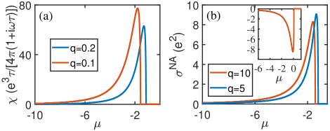
Figure 2: (Color online) (a) The second-order nonlinear longitudinal conductivity $\chi$ versus the chemical potential $\mu$ for the 1D Hamiltonian (5) in terms of parameters in (7) with time-reversal symmetry at zero temperature. Here, $t_{0}=1$, $t_{1}=6$ and $t_{2}=0.7$. (b) The linear conductivity $\sigma^{\mathrm{NA}}=\sigma_{xx}^{\mathrm{NA}}$ resulted from the NHABC versus the chemical potential $\mu$ for the 1D Hamiltonian (5) with $d_{0}=t_{3}\cos(k)$, $d_{x}=t_{0}+t_{1}\cos(k)$, $d_{y}=t_{2}\cos(k)$ and $d_{z}=0$ at zero temperature. Here, $t_{0}=1$, $t_{1}=6$, $t_{2}=2$ and $t_{3}=5$. Inset in (b): $t_{3}=-5$ so that the conductivity becomes negative.

We now focus on the longitudinal conductivity. It is a well-known fact that for a Hermitian system with symmetric energy spectra with $\varepsilon(-{\bm{k}})=\varepsilon({\bm{k}})$, there does not exist a second-order nonlinear longitudinal conductivity. However, Eq. (15) remarkably shows that a second-order nonlinear longitudinal conductivity arises in a non-Hermitian system due to the geometric structures of wave functions, i.e.,

$$\chi_{\lambda\lambda\lambda}=-\frac{e^{3}\tau}{2(1+i\omega\tau)}\int_{k}f_{0}\partial^{2}_{\lambda}\bar{A}_{\lambda}.$$ (19)

In the dc limit, $\chi$ scales as $\tau$ instead of $\tau^{2}$. At high frequencies $\omega\tau\gg 1$ but below the interband transition threshold, the prefactor in $\chi$ is independent of the scattering time so that the nonlinear longitudinal conductivity directly measures the geometric structure in the NHABC.

With time-reversal symmetry, the nonlinear longitudinal conductivity can be nonzero due to the fact that $\bar{A}_{\lambda}(-{\bm{k}})=\bar{A}_{\lambda}({\bm{k}})$ enforced by time-reversal symmetry Supplement . However, it is forced to vanish in an inversion symmetric system because inversion symmetry imposes constraints that $\bar{A}_{\lambda}(-{\bm{k}})=-\bar{A}_{\lambda}({\bm{k}})$ Supplement , making $f_{0}\partial^{2}_{\lambda}\bar{A}_{\lambda}$ an odd function. In Fig. 2(a), we plot $\chi=\chi_{xxx}$ for a 1D Hamiltonian with time-reversal symmetry, showing that a significant nonlinear longitudinal conductivity arises when the Fermi energy is close to the band edge.

Besides the nonlinear longitudinal conductivity, we are surprised to find that the NHABC can induce a linear longitudinal conductivity,

$$\sigma_{\lambda\lambda}^{\mathrm{NA}}=e^{2}\int_{k}f_{0}\partial_{\lambda}\bar{A}_{\lambda},$$ (20)

which is independent of frequencies and the scattering time. Due to the constraint imposed by time-reversal symmetry, this conductivity is forced to vanish in a time-reversal invariant system. Instead, we consider a Hamiltonian that breaks time-reversal symmetry and exhibits antisymmetric $\bar{A}$; the NHABC induced linear conductivity reaches maxima when the Fermi surface is near the band edges as illustrated in Fig. 2(b). There, the conductivity becomes negative when either $t_{3}<0$ or $q<1$.

Before closing this section, we wish to briefly discuss the NHABC induced Hall effects in two dimensions. To have nonzero linear Hall effects, one has to break time-reversal symmetry. With time-reversal symmetry, the linear Hall effects are forced to vanish, and the nonlinear Hall effects are attributed to $\bar{\Omega}_{\lambda\nu}$. To characterize the Hall current, we define three Hall pseudovectors as $d_{\lambda}^{(1)}=\epsilon_{\mu\nu}\chi_{\mu\nu\lambda}/2$ with $\epsilon_{\mu\nu}$ being the 2D Levi-Civita symbol, $d_{\lambda}^{(2)}=\epsilon_{\mu\nu}\chi_{\mu\lambda\nu}/2$, and $d_{\lambda}^{(3)}=\epsilon_{\mu\nu}\chi_{\lambda\mu\nu}/2$, which contribute to the Hall current as ${\bm{j}}_{1}^{0}=({\bm{\mathcal{E}}}\times{\bm{e}}_{z})(\bm{d}^{(1)}\cdot{\bm{\mathcal{E}}}^{*})/2$, ${\bm{j}}_{1}^{2\omega}=({\bm{\mathcal{E}}}\times{\bm{e}}_{z})(\bm{d}^{(1)}\cdot{\bm{\mathcal{E}}})/2$, ${\bm{j}}_{2}^{0}=({\bm{\mathcal{E}}^{*}}\times{\bm{e}}_{z})(\bm{d}^{(2)}\cdot{\bm{\mathcal{E}}})/2$, ${\bm{j}}_{2}^{2\omega}=({\bm{\mathcal{E}}}\times{\bm{e}}_{z})(\bm{d}^{(2)}\cdot{\bm{\mathcal{E}}})/2$, ${\bm{j}}_{3}^{0}={\bm{d}}^{(3)}[(\bm{\mathcal{E}\times\bm{\mathcal{E}}^{*}})\cdot{\bm{e}}_{z}]/2$ and ${\bm{j}}_{3}^{2\omega}=0$. The NHABC cannot yield nonzero ${\bm{d}}^{(1)}$ since $\partial_{\mu\nu}\bar{A}_{\lambda}=\partial_{\nu\mu}\bar{A}_{\lambda}$.

In summary, we have discovered anomalous coherent oscillations of a wave packet induced by the NHABC. While we demonstrate our prediction in a pseudo-Hermitian Hamiltonian, the anomalous oscillations in an ac electric field may also be observed in other non-Hermitian systems Supplement , such as a system with skin effects Yao2018PRL1 ; Xiong2018JPC , given that the dynamics of a wave packet in a non-Hermitian Hamiltonian is independent of boundary conditions Pengfei2021Arixv . In the Supplementary Material, we also propose a practical scheme with coupled resonator optical waveguides Hafezi2011NP ; Fan2004PRL ; Longhi2015SR to observe the anomalous oscillations. We further provide a generic theory, showing the existence of a NHABC induced anomalous linear longitudinal conductivity independent of the scattering time in a time-reversal symmetry broken system and a second-order anomalous nonlinear longitudinal conductivity in a time-reversal invariant system. Given that non-Hermitian physics can widely exist in disordered or strongly correlated systems (the conductivity may be insensitive to boundary conditions even for a system with skin effects Sato2021PRL ), the anomalous longitudinal conductivities may be observed in these materials. Our work thus opens a new direction for studying anomalous transport phenomena induced by NHABC in non-Hermitian systems.

In the supplementary material, we will show that the velocity of a wave packet is dependent on the Berry curvature defined by right eigenstates in non-Hermitian systems in Section S-1, present the eigenvalues of the Hamiltonian in the main text in Section S-2, discuss the effects of non-Hermitian anomalous Berry connection in a flattened Hamiltonian in Section S-3, analyze the constraints on non-Hermitian anomalous Berry connection imposed by time-reversal symmetry and inversion symmetry or two-fold rotational symmetry in Section S-4, present non-Hermitian anomalous Berry connection in other non-Hermitian models with skin effects in Section S-5, and provide an experimental scheme with coupled resonator optical waveguides in Section S-6.

I S-1. Relevant Berry curvature in non-Hermitian systems

In this section, we will show that the velocity of a wave packet is dependent on the Berry curvature defined by right eigenstates.

I.1 A. Expectation value of an observable

A quantum non-Hermitian system usually appears due to the system coupled to an environment constituting an open quantum system. Such a system is usually described by the master equation

$$i\partial_{t}\rho=[H_{eff},\rho]^{\prime}+\sum_{j}L_{j}\rho L_{j}^{\dagger},$$ (S1)

where $\rho$ is the density matrix, $[H_{eff},\rho]^{\prime}=H_{eff}\rho-\rho H_{eff}^{\dagger}$ with $H_{eff}=H_{s}-i\frac{1}{2}\sum_{j}L_{j}^{\dagger}L_{j}$ being an effective non-Hermitian Hamiltonian, $H_{s}$ is the Hamiltonian of the system, and $L_{j}$ is the jump operator. If we consider short time dynamics or consider the postselection so that the results corresponding to occurrence of a quantum jump are discarded, the dynamics is governed by

$$i\partial_{t}\rho=[H_{eff},\rho]^{\prime}.$$ (S2)

If an initial state is a pure state $|\Psi(t=0)\rangle$ [$\rho(t=0)=|\Psi(t=0)\rangle\langle\Psi(t=0)|$], then the state evolves as $\rho(t)=|\Psi(t)\rangle\langle\Psi(t)|$, where $|\Psi(t)\rangle$ evolves according to

$$i\partial_{t}|\Psi(t)\rangle=H_{eff}|\Psi(t)\rangle.$$ (S3)

The expectation value of an observable $O$ is thus given by

$$\langle O\rangle=\frac{{\text{Tr}}[O\rho(t)]}{{\text{Tr}}[\rho(t)]}=\frac{{\text{Tr}}[O|\Psi(t)\rangle\langle\Psi(t)|]}{{\text{Tr}}[|\Psi(t)\rangle\langle\Psi(t)|]}=\langle\Psi_{1}|O|\Psi_{1}\rangle,$$ (S4)

where $|\Psi_{1}\rangle=|\Psi(t)\rangle/\sqrt{\langle\Psi(t)|\Psi(t)\rangle}$. In the derivation, we have chosen an orthonormal basis including $|\Psi_{1}\rangle$ for the Hilbert space, $\beta=\{|\Psi_{1}\rangle,|\Psi_{2}\rangle,\cdots,|\Psi_{N}\rangle\}$ ($N$ denotes the dimension of the Hilbert space), so that

$${\text{Tr}}[O|\Psi(t)\rangle\langle\Psi(t)|]=\langle\Psi_{1}|O|\Psi_{1}\rangle\langle\Psi(t)|\Psi(t)\rangle+\sum_{j=2}^{N}\langle\Psi_{j}|O|\Psi(t)\rangle\langle\Psi(t)|\Psi_{j}\rangle=\langle\Psi_{1}|O|\Psi_{1}\rangle\langle\Psi(t)|\Psi(t)\rangle.$$ (S5)

This tells us that the expectation value is completely determined by the evolving state $|\Psi(t)\rangle$.

In a strongly correlated or disordered system, it has been justified in Ref. Michishita2020PRLS that the effective non-Hermitian Hamiltonian in the single-particle Green’s function corresponds to the non-Hermitian Hamiltonian in the context of an open quantum system under postselection, indicating that the expectation value of an observable of a wave packet is still determined by the evolving state $|\Psi(t)\rangle$ under the effective non-Hermitian Hamiltonian.

I.2 B. Derivation of the semiclassical equations of motion

We now provide the detailed derivation of the semiclassical dynamics of Bloch electrons (a brief version can be found in the Supplementary Material in Ref. Xu2017PRLS ). Consider a wave packet as an initial state, which can be written in terms of the right Bloch eigenstates of a non-Hermitian Hamiltonian $H$ without an external force as

$$|\Phi(t=0)\rangle=\int_{k}a(\bm{k},t=0)|\phi_{n}^{R}(\bm{k})\rangle,$$ (S6)

where $|\phi_{n}^{R}(\bm{k})\rangle=e^{i{\bm{k}}\cdot{\bm{r}}}|u_{n}^{R}(\bm{k})\rangle$ is the Bloch state with $|u_{n}^{R}(\bm{k})\rangle$ being the right eigenstate of a non-Hermitian Hamiltonian. The wave packet evolves with time as

$$|\Phi(t)\rangle=\int_{k}a(\bm{k},t)|\phi_{n}^{R}(\bm{k})\rangle,$$ (S7)

where $a({\bm{k}},t)=|a({\bm{k}},t)|e^{i\gamma({\bm{k}},t)}$ with the amplitude $|a({\bm{k}},t)|$ taking the Gaussian form centered at $\bm{k}_{c}=\int_{k}|a(\bm{k},t)|^{2}\bm{k}/\int_{k}|a(\bm{k},t)|^{2}=\int_{k}|a^{\prime}(\bm{k},t)|^{2}\bm{k}$ where $|a^{\prime}(\bm{k},t)|^{2}\equiv|a(\bm{k},t)|^{2}/\int_{k^{\prime}}|a(\bm{k}^{\prime},t)|^{2}$ (while $|a({\bm{k}},t)|$ may decrease with time in the presence of a loss term so that $\langle\Phi|\Phi\rangle=\int_{k}|a(\bm{k},t)|^{2}<1$, we can evaluate the expectation value of an observable by mutiplying a factor $1/\langle\Phi|\Phi\rangle$).

Let us first derive the expression of $\gamma({\bm{k}},t)$ which contains both dynamical and geometric phases. In the presence of an external force, the Schrödinger equation reads

$$i\partial_{t}|\psi(t)\rangle=(H-\bm{F}\cdot\hat{\bm{r}})|\psi(t)\rangle.$$ (S8)

Consider a Bloch eigenstate at $\bm{k}_{0}$ as an initial state at time $t_{0}$ and suppose that the external force is sufficiently weak so that the evolving state is still a Bloch eigenstate multiplied by a factor, that is,

$$|\psi(t)\rangle =\alpha(t)|\phi_{n\bm{k}(t)}^{R}\rangle=\alpha(t)e^{i\bm{k}(t)\cdot\bm{r}}|u_{n\bm{k}(t)}^{R}\rangle$$ (S9)

$$\bm{k}(t) =\bm{k}_{0}+\bm{F}t.$$ (S10)

We now substitute $|\psi(t)\rangle$ into the Schrödinger equation, yielding

$$i\partial_{t}|\psi(t)\rangle= ie^{i\bm{k}(t)\cdot\bm{r}}|u_{n}^{R}(\bm{k}(t))\rangle\partial_{t}\alpha(t)-\alpha(t)e^{i\bm{k}(t)\cdot\bm{r}}|u_{n}^{R}(\bm{k}(t))\rangle\bm{F}\cdot\bm{r}+i\alpha(t)e^{i\bm{k}(t)\cdot\bm{r}}\partial_{t}|u_{n}^{R}(\bm{k}(t))\rangle$$ (S11)

$$= (H-\bm{F}\cdot\hat{\bm{r}})|\psi(t)\rangle$$ (S12)

$$= \alpha(t)\hat{H}e^{i\bm{k}(t)\cdot\bm{r}}|u_{n}^{R}(\bm{k}(t))\rangle-\alpha(t)e^{i\bm{k}(t)\cdot\bm{r}}|u_{n}^{R}(\bm{k}(t))\rangle\bm{F}\cdot\bm{r}$$ (S13)

$$= \alpha(t)\varepsilon_{n}(\bm{k}(t))e^{i\bm{k}(t)\cdot\bm{r}}|u_{n}^{R}(\bm{k}(t))\rangle-\alpha(t)e^{i\bm{k}(t)\cdot\bm{r}}|u_{n}^{R}(\bm{k}(t))\rangle\bm{F}\cdot\bm{r}.$$ (S14)

We thus obtain

$$i|u_{n}^{R}(\bm{k}(t))\rangle\partial_{t}\alpha(t)=\alpha(t)\varepsilon_{n}(\bm{k}(t))|u_{n}^{R}(\bm{k}(t))\rangle-i\alpha(t)\partial_{t}|u_{n}^{R}(\bm{k}(t))\rangle.$$ (S15)

To derive the equation satisfied by $\alpha(t)$, we consider any state written as a linear combination of the left eigenstates $|u_{j}^{L}(\bm{k}(t))\rangle$ [note that $\{|u_{j}^{L}(\bm{k}(t))\rangle\}$ constitute an ordered basis, although it may not be orthogonal], that is,

$$|u^{\prime}_{\bm{k}(t)}\rangle=c_{n}^{*}|u_{n}^{L}(\bm{k}(t))\rangle+\sum_{j\neq n}c_{j}^{*}|u_{j}^{L}(\bm{k}(t))\rangle.$$ (S16)

We then multiply Eq. (S15) by $\langle u^{\prime}_{\bm{k}(t)}|$, resulting in

$$ic_{n}\partial_{t}\alpha(t) =c_{n}\alpha(t)[\varepsilon_{n}(\bm{k}(t))-i\langle u_{n}^{L}(\bm{k}(t))|\partial_{t}|u_{n}^{R}(\bm{k}(t))\rangle]-i\alpha(t)\sum_{j\neq n}c_{j}\langle u_{j}^{L}(\bm{k}(t))|\partial_{t}|u_{n}^{R}(\bm{k}(t))\rangle,$$ (S17)

where we have used the biorthogonal relation $\langle u_{m}^{L}({\bm{k}})|u_{n}^{R}({\bm{k}})\rangle=\delta_{mn}$. The final term vanishes because multiplying Eq. (S15) by $\sum_{j\neq n}c_{j}\langle u_{j}^{L}(\bm{k}(t))|$ yields

$$\alpha(t)\sum_{j\neq n}c_{j}\langle u_{j}^{L}(\bm{k}(t))|\partial_{t}|u_{n}^{R}(\bm{k}(t))\rangle=0.$$ (S18)

Thus, we obtain

$$i\partial_{t}\alpha(t) =\alpha(t)\varepsilon_{n}(\bm{k}(t))-i\alpha(t)\langle u_{n}^{L}(\bm{k}(t))|\partial_{t}|u_{n}^{R}(\bm{k}(t))\rangle=\alpha(t)\left[\varepsilon_{n}(\bm{k}(t))-\tilde{{\bm{A}}}_{n{\bm{k}}(t)}\cdot{\bm{F}}\right],$$ (S19)

yielding

$$\alpha(t)=e^{-i\int_{t_{0}}^{t}dt^{\prime}\left[\varepsilon_{n}(\bm{k}(t^{\prime}))-\tilde{{\bm{A}}}_{n}(\bm{k}(t^{\prime}))\cdot{\bm{F}}\right]},$$ (S20)

where $\tilde{{\bm{A}}}_{n}(\bm{k}(t))=i\langle u_{n}^{L}(\bm{k})|\partial_{\bm{k}}u_{n}^{R}(\bm{k})\rangle|_{\bm{k}=\bm{k}(t)}$ is the left-right Berry connection contributing to the geometric phase.

We note that in the derivation, while one can also use the right eigenvectors to generate $|u^{\prime}_{\bm{k}(t)}\rangle$, that is,

$$|u^{\prime}_{\bm{k}(t)}\rangle=b_{n}^{*}|u_{n}^{R}(\bm{k}(t))\rangle+\sum_{j\neq n}b_{j}^{*}|u_{j}^{R}(\bm{k}(t))\rangle,$$ (S21)

multiplying Eq. (S15) by this expansion cannot give us an equation as concise as Eq. (S19) due to the absence of an orthogonal relation for right eigenvectors in non-Hermitian systems [$\langle u_{m}^{R}({\bm{k}})|u_{n}^{R}({\bm{k}})\rangle$ usually does not vanish if $m\neq n$]. Note here we consider a system without exceptional points; otherwise, neither right eigenvectors nor left eigenvectors can constitute a basis for the Hilbert space.

We are now in a position to derive the center of mass of the wave packet in real space as time evolves based on Eq. (S7); the location of the wave packet is given by

$${\bm{r}}_{c}(t)$$

$$= \langle\Phi(t)|\hat{{\bm{r}}}|\Phi(t)\rangle/\langle\Phi(t)|\Phi(t)\rangle$$ (S22)

$$= \int d{\bm{r}}\int_{k}\int_{k^{\prime}}|a({\bm{k}}^{\prime},t)||a({\bm{k}},t)|e^{i\gamma({\bm{k}},t)}e^{-i\gamma({\bm{k}}^{\prime},t)}e^{-i{\bm{k}}^{\prime}\cdot{\bm{r}}}[u_{n{\bm{k}}^{\prime}}^{R}({\bm{r}})]^{\dagger}{\bm{r}}e^{i{\bm{k}}\cdot{\bm{r}}}u_{n{\bm{k}}}^{R}(\bm{r})/\langle\Phi|\Phi\rangle$$ (S23)

$$= \int d{\bm{r}}\int_{k}\int_{k^{\prime}}|a({\bm{k}}^{\prime},t)||a({\bm{k}},t)|e^{i\gamma({\bm{k}},t)}e^{-i\gamma({\bm{k}}^{\prime},t)}e^{i({\bm{k}}-{\bm{k}}^{\prime})\cdot{\bm{r}}}{\bm{r}}[u_{n{\bm{k}}^{\prime}}^{R}(\bm{r})]^{\dagger}u_{n{\bm{k}}}^{R}(\bm{r})/\langle\Phi|\Phi\rangle$$ (S24)

$$= \int_{k}\int_{k^{\prime}}\int d{\bm{r}}|a({\bm{k}}^{\prime},t)||a({\bm{k}},t)|e^{i\gamma({\bm{k}},t)}e^{-i\gamma({\bm{k}}^{\prime},t)}[u_{n{\bm{k}}^{\prime}}^{R}(\bm{r})]^{\dagger}u_{n{\bm{k}}}^{R}(\bm{r})(-i\partial_{{\bm{k}}})e^{i({\bm{k}}-{\bm{k}}^{\prime})\cdot{\bm{r}}}/\langle\Phi|\Phi\rangle$$ (S25)

$$= \int_{k}\int_{k^{\prime}}\int d{\bm{r}}e^{i({\bm{k}}-{\bm{k}}^{\prime})\cdot{\bm{r}}}|a({\bm{k}}^{\prime},t)|e^{-i\gamma({\bm{k}}^{\prime},t)}[u_{n{\bm{k}}^{\prime}}^{R}(\bm{r})]^{\dagger}i\partial_{{\bm{k}}}|a({\bm{k}},t)|e^{i\gamma({\bm{k}},t)}u_{n{\bm{k}}}^{R}(\bm{r})/\langle\Phi|\Phi\rangle$$ (S26)

$$= \int_{k}\int d{\bm{r}}|a({\bm{k}},t)|e^{-i\gamma({\bm{k}},t)}[u_{n{\bm{k}}}^{R}(\bm{r})]^{\dagger}i\partial_{{\bm{k}}}|a({\bm{k}},t)|e^{i\gamma({\bm{k}},t)}u_{n{\bm{k}}}^{R}(\bm{r})/\langle\Phi|\Phi\rangle$$ (S27)

$$= \int_{k}\int d{\bm{r}}|a({\bm{k}},t)|e^{-i\gamma({\bm{k}},t)}[u_{n{\bm{k}}}^{R}(\bm{r})]^{\dagger}\left[e^{i\gamma({\bm{k}},t)}u_{n{\bm{k}}}^{R}(\bm{r})i\partial_{{\bm{k}}}|a({\bm{k}},t)|-(\partial_{{\bm{k}}}\gamma({\bm{k}},t))|a({\bm{k}},t)|e^{i\gamma({\bm{k}},t)}u_{n{\bm{k}}}^{R}(\bm{r})+\right.$$ (S28)

$$\left.|a({\bm{k}},t)|e^{i\gamma({\bm{k}},t)}(i\partial_{{\bm{k}}})u_{n{\bm{k}}}^{R}(\bm{r})\right]/\langle\Phi|\Phi\rangle$$ (S29)

$$= \int_{k}|a({\bm{k}},t)|i\partial_{{\bm{k}}}|a({\bm{k}},t)|/\langle\Phi|\Phi\rangle-\int_{k}|a({\bm{k}},t)|^{2}(\partial_{{\bm{k}}}\gamma({\bm{k}},t))/\langle\Phi|\Phi\rangle+\int_{k}|a({\bm{k}},t)|^{2}\int d{\bm{r}}[u_{n{\bm{k}}}^{R}(\bm{r})]^{\dagger}i\partial_{{\bm{k}}}u_{n{\bm{k}}}^{R}(\bm{r})/\langle\Phi|\Phi\rangle$$ (S30)

$$= -\int_{k}|a^{\prime}({\bm{k}},t)|^{2}\partial_{{\bm{k}}}\gamma({\bm{k}},t)+\int_{k}|a^{\prime}({\bm{k}},t)|^{2}\int d{\bm{r}}[u_{n{\bm{k}}}^{R}(\bm{r})]^{\dagger}i\partial_{{\bm{k}}}u_{n{\bm{k}}}^{R}(\bm{r})$$ (S31)

$$= -\int_{k}|a^{\prime}({\bm{k}},t)|^{2}\partial_{{\bm{k}}}\gamma({\bm{k}},t)+\int_{k}|a^{\prime}({\bm{k}},t)|^{2}\langle u_{n\bm{k}}^{R}|i\partial_{\bm{k}}|u_{n\bm{k}}^{R}\rangle$$ (S32)

$$\approx -\frac{\partial\gamma({\bm{k}}_{c},t)}{\partial{\bm{k}}_{c}}+i\langle u_{n{\bm{k}}_{c}}^{R}|\partial_{{\bm{k}}_{c}}|u_{n{\bm{k}}_{c}}^{R}\rangle$$ (S33)

$$= -\frac{\partial\gamma({\bm{k}}_{c},t)}{\partial{\bm{k}}_{c}}+{\bm{A}}_{n}({\bm{k}}_{c}),$$ (S34)

where ${\bm{A}}_{n}({\bm{k}}_{c})=i\langle u_{n{\bm{k}}_{c}}^{R}|\partial_{{\bm{k}}_{c}}|u_{n{\bm{k}}_{c}}^{R}\rangle$ is the right-right Berry connection with $|u_{n{\bm{k}}_{c}}^{R}\rangle\equiv|u_{n}^{R}({\bm{k}}_{c})\rangle$. With the aid of Eq. (S20), we have

$$\gamma({\bm{k}}_{c},t)=-\int_{t_{0}}^{t}dt^{\prime}\text{Re}\left[\varepsilon_{n}({\bm{k}}(t^{\prime}))-\tilde{{\bm{A}}}_{n}({\bm{k}}(t^{\prime}))\cdot{\bm{F}}\right].$$

We thus can derive the velocity of the wave packet as

$${\bm{v}}_{c}(t_{0}) =\frac{{\bm{r}}_{c}(t_{0}+\delta t)-{\bm{r}}_{c}(t_{0})}{\delta t}$$

$$=\partial_{{\bm{k}}_{c}}\frac{\delta t\left[\text{Re}[\varepsilon_{n}({\bm{k}}_{c})]-\text{Re}[\tilde{{\bm{A}}}_{n}({\bm{k}}_{c})]\cdot{\bm{F}}\right]}{\delta t}+\frac{d{\bm{A}}_{n}({\bm{k}}_{c})}{dt}|_{t=t_{0}}$$

$$=\partial_{{\bm{k}}_{c}}\text{Re}[\varepsilon_{n}({\bm{k}}_{c})]-\partial_{{\bm{k}}_{c}}\text{Re}[\tilde{A}_{n,\nu}({\bm{k}}_{c})]\cdot F_{\nu}+\frac{d{\bm{A}}_{n}({\bm{k}}_{c})}{dt}|_{t=t_{0}}$$

$$=\partial_{{\bm{k}}_{c}}\text{Re}[\varepsilon_{n}({\bm{k}}_{c})]-(\partial_{{\bm{k}}_{c}}\text{Re}[\tilde{A}_{n,\nu}({\bm{k}}_{c})])\cdot\overset{\cdot}{k}_{c,\nu}+\frac{d{\bm{A}}_{n}({\bm{k}}_{c})}{dt}|_{t=t_{0}},$$

$$=\partial_{{\bm{k}}_{c}}\text{Re}[\varepsilon_{n}({\bm{k}}_{c})]-\partial_{{\bm{k}}_{c}}A_{n,\nu}({\bm{k}}_{c})\cdot\overset{\cdot}{k}_{c,\nu}+\frac{d{\bm{A}}_{n}({\bm{k}}_{c})}{dt}|_{t=t_{0}}+\partial_{{\bm{k}}_{c}}\left[A_{n,\nu}({\bm{k}}_{c})-\text{Re}\tilde{A}_{n,\nu}({\bm{k}}_{c})\right]\cdot\overset{\cdot}{k}_{c,\nu}$$

$$=\partial_{{\bm{k}}_{c}}\text{Re}[\varepsilon_{n}({\bm{k}}_{c})]-\overset{\cdot}{{\bm{k}}}_{c}\times\bm{\Omega}+\partial_{{\bm{k}}_{c}}\text{Re}\left[A_{n,\nu}({\bm{k}}_{c})-\tilde{A}_{n,\nu}({\bm{k}}_{c})\right]\cdot\overset{\cdot}{k}_{c,\nu}$$

$$=\partial_{{\bm{k}}_{c}}\text{Re}[\varepsilon_{n}({\bm{k}}_{c})]-\overset{\cdot}{{\bm{k}}}_{c}\times\bm{\Omega}+\partial_{{\bm{k}}_{c}}\bar{A}_{n,\nu}({\bm{k}}_{c})\cdot\overset{\cdot}{k}_{c,\nu}$$

$$=\partial_{{\bm{k}}_{c}}[\text{Re}[\varepsilon_{n}({\bm{k}}_{c})]+\bar{A}_{n,\nu}({\bm{k}}_{c})\cdot\overset{\cdot}{k}_{c,\nu}]-\overset{\cdot}{{\bm{k}}}_{c}\times\bm{\Omega},$$

where $\bar{A}_{n,\nu}({\bm{k}}_{c})\equiv\text{Re}\left[A_{n,\nu}({\bm{k}}_{c})-\tilde{A}_{n,\nu}({\bm{k}}_{c})\right]$ and $\bm{\Omega}=i\langle\nabla_{{\bm{k}}}u_{n}^{R}({\bm{k}})|\times|\nabla_{{\bm{k}}}u_{n}^{R}({\bm{k}})\rangle$. In the derivation, we have used the fact that ${\bm{F}}=\overset{\cdot}{{\bm{k}}}$. We can clearly see that the velocity of a wave packet is dependent on the right-right Berry curvature, which is independent of the left eigenstates.

II S-2. Eigenenergies of the Hamiltonian

The Hamiltonian (5) in the main text is pseudo-Hermitian, i.e., $U^{-1}HU=H^{\dagger}$ with $U=\text{diag}(\sqrt{q},1/\sqrt{q})$, and its eigenenergies are real, $\varepsilon_{\pm}=mc_{0}+\xi_{\pm}$ with $\xi_{\pm}=\pm\sqrt{ab(d_{x}^{2}+d_{y}^{2})+m^{2}c_{1}^{2}}$ and $c_{0}=(1-q^{2})/(2q)$ and $c_{1}=(1+q^{2})/(2q)$.

III S-3. Effects of non-Hermitian anomalous Berry connection in a flattened Hamiltonian

To illustrate the non-Hermitian anomalous Berry connection effects, we can take a limit and consider a flattened Hamiltonian

$$H_{\mathrm{F}}=|{u_{+}^{R}}\rangle\langle{u_{+}^{L}}|-|{u_{-}^{R}}\rangle\langle{u_{-}^{L}}|,$$ (S35)

where $|{u_{\pm}^{R}}\rangle$ and $\langle{u_{\pm}^{L}}|$ are the normalized right and left eigenstates of the Hamiltonian (5), respectively, corresponding to eigenenergy $\varepsilon_{\pm}$. For the flattened Hamiltonian, its eigenenergies are $\varepsilon_{\mathrm{F},\pm}=\pm 1$, which is independent of quasimomentum $k$ and thus the group velocity contributed by the energy dispersion vanishes. However, the non-Hermitian anomalous velocity remains the same as in the Hamiltonian (5), since it only depends on the wave functions. In this case, we can clearly see that even though the traditional semiclassical equations of motion predict the absence of motion for an electron in the presence of an external electric field, our theory indicates that the electron can still move due to the emergence of a velocity arising from the non-Hermiticity and local geometric effects. More interestingly, given that ${\bm{v}}_{\mathrm{NA}}$ is proportional to the electric field, one can control the direction of the velocity of an electron by suddenly reversing the direction of the electric field.

IV S-4. Symmetry constraints on non-Hermitian anomalous Berry connection

In this section, we explore the constraints on non-Hermitian anomalous Berry connection imposed by time-reversal symmetry and inversion or two-fold rotational symmetry.

IV.1 A. Time-reversal symmetry

For a non-Hermitian system, time-reversal and particle-hole symmetries develop into four categories Sato2019PRXS ; HZhou2019PRBS :

$$T_{\pm}H^{*}(-\bm{k})T_{\pm}^{\dagger} =\pm H(\bm{k})$$ (S36)

$$\Xi_{\pm}H^{T}(-\bm{k})\Xi_{\pm}^{\dagger} =\pm H(\bm{k}),$$ (S37)

where $T_{\pm}$ and $\Xi_{\pm}$ are unitary operators. The Hamiltonian (5) in the main text respects the time-reversal symmetry with $T_{+}$ being an identity matrix. We thus only consider the constraint imposed by $T_{+}$ with $T_{+}T_{+}^{*}=1$.

Let $|u_{n}^{R}({\bm{k}})\rangle$ and $\langle u_{n}^{L}({\bm{k}})|$ be the normalized right and left eigenstate of a non-Hermitian Hamiltonian $H({\bm{k}})$ in the $n$th band corresponding to an eigenvalue $\varepsilon_{n}({\bm{k}})$, respectively, that is, $H({\bm{k}})|u_{n}^{R}({\bm{k}})\rangle=\varepsilon_{k}|u_{n}^{R}({\bm{k}})\rangle$ and $\langle u_{n}^{L}({\bm{k}})|H({\bm{k}})=\varepsilon_{k}\langle u_{n}^{L}({k})|$. Based on the symmetry constraint, one can easily obtain

$$H(-{\bm{k}})T_{+}|u_{n}^{R}({\bm{k}})\rangle^{*} =T_{+}T_{+}^{\dagger}H(-{\bm{k}})T_{+}|u_{n}^{R}({\bm{k}})\rangle^{*}=T_{+}H^{*}({\bm{k}})|u_{n}^{R}({\bm{k}})\rangle^{*}=\varepsilon_{n}^{*}({\bm{k}})T_{+}|u_{n}^{R}({\bm{k}})\rangle^{*},$$ (S38)

and

$$(\langle u_{n}^{L}({\bm{k}})|)^{*}T_{+}^{\dagger}H(-{\bm{k}})=(\langle u_{n}^{L}({\bm{k}})|)^{*}H^{*}({\bm{k}})T_{+}^{\dagger}=\varepsilon_{n}^{*}({\bm{k}})(\langle u_{n}^{L}({\bm{k}})|)^{*}T_{+}^{\dagger},$$ (S39)

indicating that $T_{+}|u_{n}^{R}({\bm{k}})\rangle^{*}$ and $(\langle u_{n}^{L}({\bm{k}})|)^{*}T_{+}^{\dagger}$ are the right and left eigenstates of $H(-{\bm{k}})$ with eigenvalue $\varepsilon_{n}^{*}({\bm{k}})$, respectively. Since non-Hermitian anomalous Berry connection is gauge independent, we choose a gauge so that $|u_{n}^{R}(-{\bm{k}})\rangle=T_{+}|u_{n}^{R}({\bm{k}})\rangle^{*}$ and $\langle u_{n}^{L}(-{\bm{k}})|=(\langle u_{n}^{L}({\bm{k}})|)^{*}T_{+}^{\dagger}$, which fulfill the normalization condition $\langle u_{n}^{R}(-{\bm{k}})|u_{n}^{R}(-{\bm{k}})\rangle=1$ and $\langle u_{n}^{L}(-{\bm{k}})|u_{n}^{R}(-{\bm{k}})\rangle=1$. We now derive the constraints as

$$A_{n,\mu}(-{\bm{k}}) =-i\langle u_{n}^{R}(-{\bm{k}})|\partial_{\mu}u_{n}^{R}(-{\bm{k}})\rangle$$ (S40)

$$=-i(T_{+}|u_{n}^{R}({\bm{k}})\rangle^{*})^{\dagger}T_{+}|\partial_{\mu}u_{n}^{R}({\bm{k}})\rangle^{*}$$ (S41)

$$=-i(\langle u_{n}^{R}({\bm{k}})|)^{*}|\partial_{\mu}u_{n}^{R}({\bm{k}})\rangle^{*}$$ (S42)

$$=(A_{n,\mu}({\bm{k}}))^{*},$$ (S43)

and

$$\tilde{A}_{n,\mu}(-{\bm{k}}) =-i\langle u_{n}^{L}(-{\bm{k}})|\partial_{\mu}u_{n}^{R}(-{\bm{k}})\rangle=-i\langle u_{n}^{L}({\bm{k}})|^{*}T_{+}^{\dagger}T_{+}\partial_{\mu}|u_{n}^{R}({\bm{k}})\rangle^{*}=(\tilde{A}_{n,\mu}({\bm{k}}))^{*},$$ (S44)

which yield

$$\bar{\bm{A}}_{n}(-{\bm{k}})=\bar{\bm{A}}_{n}({\bm{k}}).$$ (S45)

We thus conclude that the time-reversal symmetry $T_{+}$ with $T_{+}T_{+}^{*}=1$ ensures that non-Hermitian Berry connection $\bar{\bm{A}}$ is an even function with respect to ${\bm{k}}$.

IV.2 B. Inversion symmetry or two-fold rotational symmetry

We now consider inversion symmetry or two-fold rotational symmetry which forces the Hamiltonian to respect

$$UH({-{\bm{k}}})U^{\dagger}=H({\bm{k}}),$$ (S46)

where $U$ is a unitary operator. One can easily find that $U^{\dagger}|u_{n}^{R}({\bm{k}})\rangle$ and $\langle u_{n}^{L}({\bm{k}})|U$ are the right and left eigenstates of $H(-{\bm{k}})$ corresponding to eigenenergy $\varepsilon_{n}({\bm{k}})$, respectively. By choosing a gauge so that $|u_{n}^{R}(-{\bm{k}})\rangle=U^{\dagger}|u_{n}^{R}({\bm{k}})\rangle$ and $\langle u_{n}^{L}(-{\bm{k}})|=\langle u_{n}^{L}({\bm{k}})|U$, one can derive that

$${\bm{A}}_{n}(-{\bm{k}}) = -{\bm{A}}_{n}({\bm{k}})$$ (S47)

$$\tilde{{\bm{A}}}_{n}(-{\bm{k}}) = -\tilde{{\bm{A}}}_{n}({\bm{k}}),$$ (S48)

leading to

$$\bar{{\bm{A}}}_{n}(-{\bm{k}})=-\bar{{\bm{A}}}_{n}({\bm{k}}).$$ (S49)

This tells us that inversion symmetry maintains that non-Hermitian anomalous Berry connection is antisymmetric with respect to ${\bm{k}}$. If a system has both time-reversal symmetry $T_{+}$ and inversion or two-fold rational symmetry, then non-Hermitian anomalous Berry connection is forced to vanish.

IV.3 C. $C_{2}\mathcal{T}$ or ${\mathcal{PT}}$ symmetry

For the $C_{2}\mathcal{T}$ (product of two-fold rotational symmetry and time-reversal symmetry) or ${\mathcal{PT}}$ (product of inversion symmetry and time-reversal symmetry) symmetry, the Hamiltonian should satisfy

$$UT_{+}H({\bm{k}})^{*}(UT_{+})^{\dagger}=H({\bm{k}}),$$ (S50)

where $UT_{+}$ is a unitary operator. We consider the case that $(UT_{+})(UT_{+})^{*}=1$. Similarly, one can find that $UT_{+}|u_{n}^{R}({\bm{k}})\rangle^{*}$ and $(\langle u_{n}^{L}({\bm{k}})|)^{*}(UT_{+})^{\dagger}$ are the right and left eigenstates of $H({\bm{k}})$ corresponding to eigenenergy $\varepsilon_{n}^{*}({\bm{k}})$, respectively. If a system is in a $C_{2}\mathcal{T}$ or ${\mathcal{PT}}$ symmetric state, that is, $UT_{+}|u_{n}^{R}({\bm{k}})\rangle^{*}={\alpha}^{*}|u_{n}^{R}({\bm{k}})\rangle$ and $\langle u_{n}^{L}({\bm{k}})|^{*}(UT_{+})^{\dagger}=\alpha\langle u_{n}^{L}({\bm{k}})|$ with $|\alpha|=1$, then one can easily derive

$${A}_{n,\mu}({\bm{k}}) = i\alpha^{*}\partial_{\mu}\alpha-(A_{n,\mu}({\bm{k}}))^{*}$$ (S51)

$$\tilde{A}_{n,\mu}({\bm{k}}) = i\alpha^{*}\partial_{\mu}\alpha-(\tilde{A}_{n,\mu}({\bm{k}}))^{*},$$ (S52)

so that

$$\bar{{\bm{A}}}_{n}({\bm{k}})=-\bar{{\bm{A}}}_{n}({\bm{k}}),$$ (S53)

forcing non-Hermitian anomalous Berry connection to vanish.

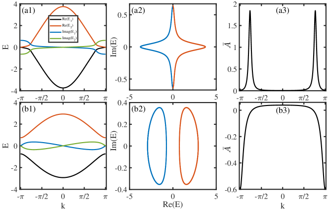
Figure S1: (Color online) (a1)(b1) Real and imaginary parts of energy spectra with respect to quasimomenta $k$ for the Hamiltonian (S54) with the corresponding energy spectra in the complex plane plotted in (a2) and (b2), respectively. (a3)(b3) NHABC as a function of quasimomenta $k$. In (a1-a3), $t_{1}=2$, $t_{2}=1$, $t_{3}=0.8$ and $\gamma=4/3$, and in (b1-b3), $t_{1}=2$, $t_{2}=1$, $t_{3}=0$ and $\gamma=4/3$.

V S-5. Non-Hermitian anomalous Berry connections in other models

In the main text, we consider a model with pseudo-Hermiticity symmetry that exhibits large NHABC. In fact, the NHABC is generically nonzero in a non-Hermitian system. Here, we show that NHABC can be large in other well-known models with skin effects Tony2016S ; Yao2018PRL1S ,

$$H(k)=d_{x}\sigma_{x}+(d_{y}+i\gamma/2)\sigma_{y},$$ (S54)

where $d_{x}=t_{1}+(t_{2}+t_{3})\cos(k)$ and $d_{y}=(t_{2}-t_{3})\sin(k)$ with $t_{1}$, $t_{2}$, $t_{3}$ and $\gamma$ being real parameters describing the corresponding hopping strength.

To show that NHABC has significant effects, we consider two typical cases with $t_{1}=2$, $t_{2}=1$, $t_{3}=0.8$ and $\gamma=4/3$, and $t_{1}=2$, $t_{2}=1$, $t_{3}=0$ and $\gamma=4/3$. The system exhibits non-Hermitian skin effects under open boundary conditions since the energy spectra in the complex plane in momentum space [see Fig. S1(a2) and (b2)] have nonzero winding. Figure S1(a3) and (b3) further illustrate that the NHABC is also in the order of one in these systems, similar to the case shown in Fig. 1(a) in the main text for a pseudo-Hermitian Hamiltonian.

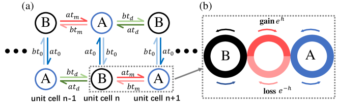
Figure S2: (Color online) (a) Lattice configurations to realize the Hamiltonian (5) in the main text. Circles labeled by A and B represent site resonators. The effective hopping between the site resonators is generated by a link waveguide (red circle) connecting two neighboring site resonators (black and blue circles) as shown in (b). When gain and loss are involved in link waveguides, the required asymmetric hopping can be realized.

VI S-6. An experimental scheme with coupled resonator optical waveguides

To experimentally realize the Hamiltonian (5) with $d_{z}=d_{0}=0$, $d_{x}=t_{0}+t_{1}\cos k$ and $d_{y}=t_{2}\sin k$, we first write down the Hamiltonian in real space

$$H=\sum_{n} \left[(\begin{array}[]{cc}|A_{n}\rangle&|B_{n}\rangle\end{array})\left(\begin{array}[]{cc}0&at_{0}\\ bt_{0}&0\\ \end{array}\right)\left(\begin{array}[]{c}\langle A_{n}|\\ \langle B_{n}|\end{array}\right)+(\begin{array}[]{cc}|A_{n}\rangle&|B_{n}\rangle\end{array})\left(\begin{array}[]{cc}0&at_{d}\\ bt_{m}&0\\ \end{array}\right)\left(\begin{array}[]{c}\langle A_{n+1}|\\ \langle B_{n+1}|\end{array}\right)\right.$$ (S65)

$$\left.+(\begin{array}[]{cc}|A_{n+1}\rangle&|B_{n+1}\rangle\end{array})\left(\begin{array}[]{cc}0&at_{m}\\ bt_{d}&0\\ \end{array}\right)\left(\begin{array}[]{c}\langle A_{n}|\\ \langle B_{n}|\end{array}\right)\right],$$ (S71)

where $|A_{n}\rangle$ and $|B_{n}\rangle$ denote the state at site A and B in the $n$th unit cell, respectively, $t_{m}=(t_{1}+t_{2})/2$ and $t_{d}=(t_{1}-t_{2})/2$. To realize the Hamiltonian in coupled-resonator optical waveguides (CROWs), we consider a configuration for site resonators and link waveguides as illustrated in Fig. S2(a), where A and B sites are interchanged in positions between two neighboring unit cells to realize the next-nearest neighbor hopping between two neighboring unit cells. The hopping between two neighboring sites are implemented by coupling two site resonators (denoted by black and blue circles) with a link waveguide (denoted by a red circle), as shown in Fig. S2(b). In the non-Hermitian case, the asymmetric hopping between two sites can be realized by applying either gain $e^{h}$ or loss $e^{-h}$ over half circle for a light travelling in a link waveguide Longhi2015SRS . For instance, consider a light propagating counterclockwise in a site resonator and a gain in the upper semicircle and a loss in the lower semicircle in a link waveguide (see Fig. S2(b)). Such a gain or loss changes the transfer matrix of a link waveguide from left to right by a factor of $e^{h}$, resulting in an effective hopping from $\kappa$ to $\kappa e^{h}$, where $\kappa$ refers to the hopping when $h=0$. Similarly, the effective hopping from right to left is modified by a factor of $e^{-h}$.

The dynamics of a wave function is governed by

$$i\partial_{t}|\Psi\rangle=H|\Psi\rangle+\sum_{n}(\omega_{n}-\bar{\omega})\left(\begin{array}[]{c}a_{n}|A_{n}\rangle\\ b_{n}|B_{n}\rangle\end{array}\right)-i\gamma|\Psi\rangle,$$ (S72)

where

$$|\Psi\rangle=\sum_{n}\left(\begin{array}[]{c}a_{n}|A_{n}\rangle\\ b_{n}|B_{n}\rangle\end{array}\right)$$ (S73)

with $a_{n}$ ($b_{n}$) denoting the electric field of the light in the A (B) site resonator in the $n$th unit cell, $\gamma$ is the global decay rate of the field, and $\omega_{n}=\bar{\omega}+\delta\omega_{n}$ represents the resonant frequency of each site resonator. To simulate an external gradient potential, each site resonator is engineered to have a resonant frequency of $\bar{\omega}+\delta\omega_{n}$ with $\delta\omega_{n}=\mathcal{E}n$. One can also realize an external ac electric field by controlling local refractive index Fan2004PRLS ; Longi2007PRES .

References

• (1) R. El-Ganainy, K. G. Makris, M. Khajavikhan, Z. H. Musslimani, S. Rotter, and D. N. Christodoulides, Nat. Phys. 14, 11 (2018).
• (2) Y. Xu, Front. Phys. 14, 43402 (2019).
• (3) D.-W. Zhang, Y.-Q. Zhu, Y. X. Zhao, H. Yan, and S.-L. Zhu, Adv. Phys. 67, 253 (2019).
• (4) Y. Ashida, Z. Gong, and M. Ueda, Adv. Phys. 69, 249 (2020).
• (5) E. J. Bergholtz, J. C. Budich, and F. K. Kunst, Rev. Mod. Phys. 93, 015005 (2021).
• (6) B. Zhen, C. W. Hsu, Y. Igarashi, L. Lu, I. Kaminer, A. Pick, S.-L. Chua, J. D. Joannopoulos, and M. Soljačić, Nature 525, 354 (2015).
• (7) Y. Xu, S.-T. Wang, and L.-M. Duan, Phys. Rev. Lett. 118, 045701 (2017).
• (8) A. Cerjan, M. Xiao, L. Yuan, and S. Fan, Phys. Rev. B 97, 075128 (2018).
• (9) H.-Y Zhou, C. Peng, Y. Yoon, C. W. Hsu, K. A. Nelson, L. Fu, J. D. Joannopoulos, Soljačić, and B. Zhen, Science 359, 1009 (2018).
• (10) J. Carlström and E. J. Bergholtz, Phys. Rev. A 98, 042114 (2018).
• (11) Z. Yang and J. Hu, Phys. Rev. B 99, 041202(R) (2019).
• (12) H.-Q. Wang, J.-W. Ruan, and H.-J. Zhang, Phys. Rev. B 99, 075130 (2019).
• (13) S. K. Özdemir, S. Rotter, F. Nori, and L. Yang, Nat. Mater. 18, 783 (2019).
• (14) A. Cerjan, S. Huang, M. Wang, K. P. Chen, Y. Chong, and M. C. Rechtsman, Nat. Photon 13, 623 (2019).
• (15) K. Kawabata, T. Bessho, and M. Sato, Phys. Rev. Lett. 123, 066405 (2019).
• (16) X.-F. Zhang, K. Ding, X.-J. Zhou, J. Xu, and D.-F. Jin, Phys. Rev. Lett. 123, 237202 (2019).
• (17) J. Hou, Z. Li, X.-W. Luo, Q. Gu, and C. Zhang, Phys. Rev. Lett. 124, 073603 (2020).
• (18) Z. Yang, C.-K. Chiu, C. Fang, and J. Hu, Phys. Rev. Lett. 124, 186402 (2020).
• (19) K.-K. Wang, L. Xiao, J. C. Budich, W. Yi, and P. Xue, Phys. Rev. Lett. 127, 026404 (2021).
• (20) V. Kozii and L. Fu, arXiv:1708.05841 (2017).
• (21) A. A. Zyuzin and A. Yu. Zyuzin, Phys. Rev. B 97, 041203(R) (2018).
• (22) T. Yoshida, R. Peters, and N. Kawakami, Phys. Rev. B 98, 035141 (2018).
• (23) P.-L. Zhao, A.-M. Wang, and G.-Z. Liu, Phys. Rev. B 98, 085150 (2018).
• (24) T. Yoshida, R. Peters, N. Kawakami, and Y. Hatsugai, Phys. Rev. B 99, 121101(R) (2019).
• (25) Y. Nagai, Y. Qi, H. Isobe, V. Kozii, and L. Fu, Phys. Rev. Lett. 125, 227204 (2020).
• (26) N. Okuma and M. Sato, Phys. Rev. Lett. 126, 176601 (2021).
• (27) Y.-L. Tao, T. Qin, and Y. Xu, arXiv:2111.03348 (2021).
• (28) M.-C. Chang and Q. Niu, Phys. Rev. Lett. 75, 1348 (1995).
• (29) G. Sundaram and Q. Niu, Phys. Rev. B 59, 14915 (1999).
• (30) D. Xiao, J. Shi, and Q. Niu, Phys. Rev. Lett. 95, 137204 (2005).
• (31) D. Xiao, M.-C. Chang, and Q. Niu, Rev. Mod. Phys. 82, 1959 (2010).
• (32) Y. Gao, S. A. Yang, and Q. Niu, Phys. Rev. Lett. 112, 166601 (2014).
• (33) I. Sodemann and L. Fu, Phys. Rev. Lett. 115, 216806 (2015).
• (34) N. Silberstein, J. Behrends, M. Goldstein, and R. Ilan, Phys. Rev. B 102, 245147 (2020).
• (35) See the Supplementary Material.
• (36) C. Blohmann, Eur. Phys. J. C 30, 435 (2003).
• (37) Y.-Q. Zhu, W. Zheng, S.-L. Zhu, and G. Palumbo, Phys. Rev. B 104, 205103 (2021).
• (38) A. Mostafazadeh, J. Math. Phys. 43, 205 (2002).
• (39) K. Zhang, Z. Yang, and C. Fang, Phys. Rev. Lett. 125, 126402 (2020).
• (40) N. Okuma, K. Kawabata, K. Shiozaki, and M. Sato, Phys. Rev. Lett. 124, 086801 (2020).
• (41) D. S. Borgnia, A. J. Kruchkov, and R.-J. Slager, Phys. Rev. Lett. 124, 056802, (2020).
• (42) S. Yao and Z. Wang, Phys. Rev. Lett. 121, 086803 (2018).
• (43) Y. Xiong, J. Phys. Commun. 2, 035043 (2018).
• (44) L. Mao, T. Deng, and P. Zhang, arXiv:2104.09896 (2021).
• (45) M. Hafezi, E. A. Demler, M. D. Lukin, and J. M. Taylor, Nat. Phys. 7, 907 (2011).
• (46) M. F. Yanik and S. Fan, Phys. Rev. Lett. 92, 083901 (2004).
• (47) S. Longhi, D. Gatti, and G. D. Valle, Sci. Rep. 5, 13376 (2015).

References

• (1) Y. Michishita and R. Peters, Phys. Rev. Lett. 124, 196401 (2020).
• (2) Y. Xu, S.-T. Wang, and L.-M. Duan, Phys. Rev. Lett. 118, 045701 (2017).
• (3) K. Kawabata, K. Shiozaki, M. Ueda, and M. Sato, Phys. Rev. X 9, 041015 (2019).
• (4) H. Zhou and J. Y. Lee, Phys. Rev. B 99, 235112 (2019).
• (5) T. E. Lee, Phys. Rev. Lett. 116, 133903 (2016).
• (6) S. Yao and Z. Wang, Phys. Rev. Lett. 121, 086803 (2018).
• (7) S. Longhi, D. Gatti, and G. D. Valle, Sci. Rep. 5, 13376 (2015).
• (8) M. F. Yanik and S. Fan, Phys. Rev. Lett. 92, 083901 (2004).
• (9) S. Longhi, Phys. Rev. E 75, 026606 (2007).